UK Carbon Price Dynamics: Long-Memory Effects and AI-Based Forecasting

Abstract

This study examines the price dynamics of the UK Emission Trading Scheme (UK ETS) by integrating advanced computational methods, including deep learning and statistical modelling, to analyze and simulate carbon market behaviour. By analyzing long-memory effects and price volatility, it assesses whether UK carbon prices align with theoretical expectations from carbon pricing mechanisms and market efficiency theories. Findings indicate that UK carbon prices exhibit persistent long-memory effects, contradicting the Efficient Market Hypothesis, which assumes price movements are random and fully reflect available information. Furthermore, regulatory interventions exert significant downward pressure on prices, suggesting that policy uncertainty disrupts price equilibrium in cap-and-trade markets. Deep learning models, such as Time-series Generative Adversarial Networks (TGANs) and adjusted fractional Brownian motion, outperform traditional approaches in capturing price dependencies but are prone to overfitting, highlighting trade-offs in AI-based forecasting for carbon markets. These results underscore the need for predictable regulatory frameworks, hybrid pricing mechanisms, and data-driven approaches to enhance market efficiency. By integrating empirical findings with economic theory, this study contributes to the carbon finance literature and provides insights for policymakers on improving the stability and effectiveness of emissions trading systems.

1. Introduction

As the evidence of climate change continues to mount, it is clear that this challenge is multifaceted and cannot be easily addressed through traditional policy approaches. To reduce climate-related risks, many countries have implemented national and regional emissions trading systems. These mechanisms aim to make polluters internalize the external costs of their emissions [1]. The goal is to incentivize emissions reductions by making it economically advantageous for companies to invest in cleaner technologies and practices [2]. The European Union Emissions Trading System (EU ETS), established in 2005, has served as a model for similar initiatives worldwide. Following Brexit, the UK launched its own UK Emissions Trading Scheme (UK ETS) in January 2021, providing an independent framework to regulate carbon emissions through market-based mechanisms. The UK ETS operates similarly to the EU ETS as a cap-and-trade system but exhibits distinct market dynamics due to regulatory divergence, supply mechanisms, and domestic economic factors [3]. UK carbon permits, officially known as UK allowances (UKAs), are tradable certificates within the UK ETS. Each UKA represents the right to emit one tonne of carbon dioxide (CO₂) or equivalent greenhouse gases. Unlike other commodity markets, carbon permits are influenced not only by supply and demand fundamentals but also by regulatory cycles, volatility clustering [4], economic policy uncertainty [5,6], and climate policy uncertainty [7]. Accurate carbon price forecasting is essential for increasing market transparency, supporting decarbonization strategies, and reducing financial risk from carbon exposure.

Despite the importance of carbon price forecasting, existing models face significant limitations. Carbon markets, as a nexus of environmental and financial considerations, present data characteristics (volatility clustering, mean reversion, and structural breaks) similar to those in financial markets [8]. The self-similarity in carbon price fluctuations suggests that long-term memory effects fundamentally shape market behaviour [9]. However, previous research has largely overlooked these persistent structures, leading to suboptimal predictive accuracy and potentially hindering market efficiency [10]. Regarding the process of synthetic data generation, conventional approaches, while effective in certain aspects, may struggle to capture the full complexity and nuances of real-world carbon price time series [11]. Studies using synthetic data often rely on limited validation techniques, primarily focusing on basic statistical properties [12]. This raises concerns about the reliability and generalizability of findings based on synthetic data. This study addresses these research gaps by integrating advanced computational techniques—particularly deep learning models such as Time-series Generative Adversarial Networks (TGANs)—to analyze and replicate UK carbon price dynamics.

Several key factors drive the decision to focus this study on the UK ETS market. First, regulatory distinctions following Brexit have led to a divergence between the UK ETS and the EU ETS, resulting in separate allowance auctions, price floors, and regulatory interventions [13]. These differences create unique price behaviours that cannot be directly inferred from EU ETS trends. Second, the UK ETS operates as a relatively new market compared to the EU ETS, leading to distinct liquidity constraints and price formation mechanisms. Examining price dynamics in a smaller, less liquid market provides valuable insights applicable to other emerging carbon trading systems. Lastly, the UK economy features a unique energy mix, industrial composition, and carbon reduction commitments that set it apart from other ETS markets. The impact of macroeconomic variables, energy policy decisions, and carbon reduction targets on UK carbon pricing necessitates a focused analysis [14]. By examining the UK ETS, this study not only enhances the understanding of an increasingly important carbon market but also provides a framework applicable to other emissions trading systems globally. The methodology employed here—combining long-memory modelling with deep learning approaches—can be extended to other carbon markets to improve forecasting accuracy and policy evaluation.

This research aims to explore the structural and predictive dynamics of UK carbon markets by addressing three key objectives. First, it investigates the persistence of long-memory effects in carbon prices, challenging the Efficient Market Hypothesis (EMH) [15]. By quantifying self-similar price behaviour using the Hurst exponent and fractional Brownian motion (fBm), this study aims to enhance the understanding of non-random price dependencies often overlooked by traditional models. Second, this study evaluates the effectiveness of deep learning models, particularly TGAN, in capturing the intricate temporal dependencies and volatility inherent in carbon price data. Finally, it compares the predictive accuracy of traditional econometric models with advanced machine learning approaches to assess their suitability for carbon market forecasting. By exploring innovative methodologies, this research seeks to refine forecasting methodologies and provide a more comprehensive understanding of carbon market price dynamics.

This research makes several novel contributions to the field of carbon market analysis by integrating advanced methodologies and providing empirical insights into UK carbon price dynamics. Unlike previous studies focusing on short-term price fluctuations [8], this study emphasizes structural price properties. It explores the role of long-range dependencies in shaping future price behaviour, challenging conventional assumptions of market efficiency. This study uses Rescaled Range (R/S) analysis to estimate the Hurst exponent and applies fractional Brownian motion (fBm) to generate synthetic data. These methods provide empirical evidence of self-similarity and long-term dependence in UK carbon prices. This finding challenges the Efficient Market Hypothesis in carbon trading, as price signals may not always align with fundamental abatement costs. A key innovation is the adjusted fBm model, which uses spectral scaling from the empirical covariance matrix to better match real market dynamics. This study addresses forecasting limitations related to missing data and seasonality by applying linear interpolation and Locally Estimated Scatterplot Smoothing (LOESS)-based decomposition [16]. This improves the quality and consistency of the input data.

To enhance forecasting capabilities, the research employs TGAN-based synthetic data generation, demonstrating its effectiveness in capturing complex market dependencies and improving scenario analysis. A novel validation framework is also introduced, where a Long Short-Term Memory (LSTM) regression model is used to assess the predictive power of synthetic data beyond conventional statistical comparisons. To validate the relevance of the proposed methodology, deep learning-based predictions are benchmarked against those generated by a traditional econometric model. This model is the Autoregressive Integrated Moving Average with Exogenous Variables (ARIMAX), which serves as a secondary reference. Despite differences in the underlying modelling frameworks, this comparison provides a contextual basis for assessing the predictive performance of synthetic data-driven forecasting methods. This study evaluates the advantages of deep learning models, such as TGAN, over traditional econometric approaches. In doing so, it advances synthetic data modelling for carbon markets and offers practical insights for both policymakers and market participants. Although Artificial Intelligence (AI)-based models like TGAN and long-memory processes are not new in financial forecasting, their use for synthetic data generation and predictive validation in carbon markets, especially the UK ETS, is still limited. This study bridges that gap by integrating these methods into a framework tailored to emissions trading dynamics.

The remainder of this study is structured as follows: Section 2 reviews the literature on carbon pricing models, highlighting their strengths and limitations. Section 3 presents the theoretical analysis and research hypotheses. Section 4 details the methodology, including data sources, preprocessing techniques, and modelling frameworks. Section 5 provides the empirical results and analysis, and Section 6 concludes with the study’s findings and discusses the research implications.

2. Literature Review

The study of carbon pricing mechanisms has gained increasing attention due to their critical role in climate policy and market efficiency [7]. Research on carbon pricing employs various methods, each with distinct strengths and limitations, often combining several approaches to gain a comprehensive understanding of this complex policy instrument. Traditional time-series models, such as ARIMA (Autoregressive Integrated Moving Average), ARIMAX (Autoregressive Integrated Moving Average with Exogenous Variables), and GARCH (Generalized Autoregressive Conditional Heteroskedasticity), remain popular due to their transparency, ease of interpretation, and strong statistical underpinnings [17,18]. These models are particularly useful for identifying trends, volatility, and autoregressive patterns in carbon markets. However, their reliance on linear assumptions and stationarity constraints limits their capacity to capture the non-linear, dynamic, and evolving nature of carbon pricing. Additionally, these models often fail to accommodate regime shifts, structural breaks, and complex seasonal interactions commonly observed in carbon markets.

Computable General Equilibrium (CGE) models offer a broader macroeconomic perspective by simulating the economy-wide impacts of carbon pricing policies [19]. They are grounded in economic theory and are useful for policy evaluation and scenario analysis. However, their accuracy strongly depends on parameter calibration, especially elasticity assumptions. This leads to significant variation across studies and raises concerns about robustness and replicability.

In contrast, machine learning (ML) and deep learning (DL) models such as Long Short-Term Memory (LSTM), Temporal Convolutional Networks (TCNs), Support Vector Regression (SVR), and Spiking Neural Networks (SNNs) provide powerful tools to model non-linear, high-dimensional, and non-stationary time series [20,21,22,23]. These models can detect subtle temporal interactions and adaptive patterns that traditional models may miss. However, they suffer from a lack of interpretability, potential overfitting, high computational cost, and sensitivity to hyperparameter tuning [24]. Moreover, their performance often depends on the availability of large, high-quality datasets—an ongoing challenge in emerging carbon markets.

Experimental and quasi-experimental approaches, such as difference-in-differences, randomized controlled trials, and event studies, provide rigorous empirical evidence on the causal effects of carbon pricing policies [25,26,27]. While these methods are essential for policy evaluation, they are difficult to implement in real-world contexts due to ethical, political, and logistical constraints. Additionally, quasi-experimental designs may not fully control for confounding variables and can be sensitive to methodological decisions, such as the choice of event windows.

While the literature on carbon price modelling spans a diverse set of methodological paradigms—ranging from traditional econometrics to computable general equilibrium (CGE) frameworks and machine learning (ML)/deep learning (DL) models—it rarely offers a structured comparative synthesis that evaluates their respective strengths and limitations in an integrated manner. Such a synthesis is crucial to justify the need for hybrid approaches in complex policy domains like carbon markets. To address this gap and substantiate our methodological framework,

Table 1. Comparative evaluation of modelling paradigms for carbon price forecasting.

Analytical Criterion	Traditional Econometric Models	Computable General Equilibrium (CGE) Models	Machine/Deep Learning Models
Theoretical foundation	Strong (economically grounded)	Very strong (macroeconomic equilibrium theory)	Limited (primarily data-driven)
Interpretability	High (parameter-based, transparent)	High (clearly structured assumptions)	Low (black-box characteristics)
Predictive accuracy	Moderate (limited for non-linear or volatile series)	Weak (low temporal granularity)	High (strong in non-linear and high-dimensional data
Ability to capture long memory and seasonality	Limited (short autoregressive memory)	Absent	Excellent (designed for long-range temporal dependencies)
Robustness and stability	High (under classical assumptions)	Sensitive to calibration and elasticities	Medium–Low (overfitting, parameter sensitivity)
Data requirements	Low to moderate	Very high (macro-aggregated data)	High (large, high-frequency datasets needed)
Adaptability to emerging carbon markets	Low (requires stationarity, linearity)	Very low (static, scenario-based)	High (flexible to structural change and noise)
Policy relevance	High (interpretable, scenario-driven)	High (macro policy analysis)	Low (difficult to translate into actionable recommendations)
Key limitations	Poor handling of non-linearity and regime shifts	Inflexible, overly abstract	Lack of transparency, risk of overfitting, training instability
Core strengths	Transparent, interpretable, easy to validate	Theoretically rigorous, system-wide simulations	High-dimensional learning, adaptability, forecasting power

presents a comparative matrix of the three dominant modelling paradigms: (i) traditional econometric models, (ii) CGE-based macroeconomic simulations, and (iii) ML/DL-based data-driven architectures. The comparison spans theoretical rigour, interpretability, predictive capacity, robustness, and policy relevance—dimensions essential to the modelling of price dynamics in emerging emissions trading systems (ETS).

Table 1 clearly reveals that no single paradigm is sufficient in isolation to model the non-linearities, regulatory feedbacks, and temporal complexities inherent in carbon pricing. Therefore, this study adopts a hybrid modelling framework that integrates the theoretical transparency of traditional models with the adaptive and high-dimensional capabilities of deep learning. This integration ensures both empirical robustness and practical relevance for stakeholders in carbon markets. This integrated perspective is implemented by benchmarking the performance of transformer-based Generative Adversarial Networks (TGAN) and fractional Brownian motion (fBm) against a traditional ARIMAX baseline. The comparative framework enables a systematic evaluation of the forecasting improvements introduced by deep learning methods, while preserving the interpretability and theoretical coherence characteristic of traditional models. This hybrid approach is particularly well-suited to emerging carbon markets, where the need for predictive accuracy must be balanced with policy relevance and methodological transparency.

3. Theoretical Background and Hypotheses Development

3.1. Introduction to Carbon Pricing Mechanisms

Carbon pricing mechanisms are essential for addressing climate change by internalizing the external costs of greenhouse gas emissions. These mechanisms can be broadly classified into two theoretical models: Pigouvian taxation (carbon tax) and cap-and-trade systems. Each model has distinct characteristics, advantages, and challenges, critical for policymakers aiming to reduce carbon emissions effectively.

The Pigouvian tax, named after economist Arthur Pigou, is designed to correct the market failure caused by negative externalities, such as carbon emissions [28]. By taxing carbon emissions, the government incentivizes emitters to reduce their carbon footprint, thereby internalizing the external costs associated with pollution. This approach is grounded in the principle that polluters should pay for the damage they cause to the environment, which aligns with the “polluter pays” principle [29]. Research indicates that a well-structured carbon tax can yield a “double dividend” [30]. The first dividend is the environmental benefit from reduced emissions, while the second is the potential for economic growth by reinvesting tax revenues into green technologies and infrastructure. For instance, studies have shown that carbon taxes can stimulate innovation in low-carbon technologies, leading to long-term economic benefits [31]. However, the effectiveness of a carbon tax can be influenced by its design, including the tax rate and the scope of emissions covered [32]. Moreover, implementing a carbon tax can face public resistance, often due to concerns about its regressive nature, where lower-income households disproportionately bear the burden of increased energy costs [33]. To mitigate this, policymakers can consider revenue recycling strategies, where tax revenues are used to offset costs for vulnerable populations or to fund renewable energy projects [34]. In a carbon tax system, price stability results from the government setting a fixed tax per ton of carbon emitted. This ensures that carbon prices remain stable and predictable, allowing businesses to make informed investment decisions more confidently. However, while the tax provides economic predictability, it does not directly cap emissions, meaning that firms can continue polluting if willing to pay the tax. As a result, while carbon pricing remains stable, the actual level of emissions remains uncertain, as it depends on how firms respond to the financial incentive to reduce pollution.

The UK Emissions Trading Scheme (UK ETS), which serves as the empirical basis for this study, operates under a cap-and-trade model, where firms trade emission allowances within a government-imposed cap. In contrast to carbon taxes, cap-and-trade systems establish a market for carbon emissions by setting a limit (cap) on total emissions and allowing companies to buy and sell allowances for emissions. This market-based approach incentivizes companies to reduce their emissions below their allocated cap, as they can sell excess allowances for profit. The cap-and-trade model is rooted in the Coase theorem, which suggests that market mechanisms can lead to efficient outcomes in the presence of externalities, provided property rights are well-defined [35]. Cap-and-trade systems have been implemented in various regions with mixed results. While they can effectively reduce emissions, their success often depends on the robustness of the regulatory framework and the initial allocation of allowances [32]. For example, studies have shown that cap-and-trade can significantly reduce emissions when combined with complementary policies, such as renewable energy mandates [36]. However, challenges such as market volatility and the potential for “leakage”, where emissions are transferred to regions with less stringent regulations, can undermine the effectiveness of cap-and-trade systems [37]. Unlike a carbon tax, which sets a fixed price on emissions, a cap-and-trade system ensures that total emissions remain capped while allowing prices to fluctuate based on market conditions. In this system, market forces determine the price of emission allowances through supply and demand, creating a dynamic pricing mechanism. Ideally, in a well-functioning market, the price of these allowances should reflect the marginal cost of abatement—the cost required to reduce one additional unit of emissions—ensuring an economically efficient approach to emissions reduction.

In conclusion, both carbon taxes and cap-and-trade systems aim to reduce greenhouse gas emissions but do so through different mechanisms. Carbon taxes provide price certainty, allowing businesses to plan for future costs, while cap-and-trade offers certainty in emission reductions but can lead to price volatility in allowance markets [32]. The choice between these mechanisms often depends on political, economic, and social contexts, as well as the specific environmental goals of a region. Empirical evidence suggests that a hybrid approach, integrating elements of both carbon taxation and cap-and-trade, may yield the best outcomes [31]. For instance, combining a carbon tax with a cap-and-trade system can stabilize prices while ensuring that emission reduction targets are met [38]. Furthermore, the design of these mechanisms should consider equity implications to ensure that the burden of climate policies does not disproportionately affect low-income communities [34]. Policymakers must carefully design these mechanisms to maximize environmental benefits while minimizing economic disruptions and ensuring social equity.

3.2. Efficient Market Hypothesis (EMH) and Carbon Pricing

The effectiveness of a cap-and-trade system depends on how efficiently carbon prices reflect market fundamentals. According to the EMH, prices in a well-functioning market should fully reflect all available information at any given time [15]. Within this theoretical framework, carbon prices should adjust instantly and unbiasedly to new information, ensuring allocative efficiency in emissions trading schemes (ETS). Several canonical conditions underpin this idealized efficiency: high liquidity, broad participation, information transparency, and regulatory stability [39].

However, while EMH offers a foundational lens, its assumptions often fail to hold empirically in carbon markets. Studies have documented departures from random walk behaviour in carbon price series, indicating serial correlation, long memory, and mean-reverting structures [40,41,42]. These findings are inconsistent with the weak-form EMH and suggest the presence of persistent price dynamics potentially exploitable by informed traders. Moreover, carbon markets are relatively young, politically contingent, and structurally mediated—features that limit the applicability of classical market efficiency assumptions.

Recent literature advances alternative explanations for these inefficiencies rooted in behavioural and institutional economics. A growing body of research models carbon price dynamics using regime-switching frameworks, where markets alternate between low- and high-volatility states due to shifts in regulatory signals, policy uncertainty, or macroeconomic shocks [43]. These non-linear dynamics deviate from the EMH’s assumption of a single, stable equilibrium process.

Moreover, the financialization of carbon markets has introduced speculative pressures, with increased participation from financial actors seeking portfolio diversification or arbitrage opportunities [44]. This can decouple carbon prices from underlying abatement cost fundamentals, reducing the environmental integrity of price signals. Investor heterogeneity—in expectations, risk tolerance, and time horizons—further contributes to asymmetric responses to information, while behavioural biases such as herding, overreaction to policy news, or confirmation bias can generate price anomalies [45].

Institutional design also plays a central role. Factors such as allocation mechanisms (e.g., free versus auctioned allowances), banking and borrowing rules, and market segmentation across jurisdictions influence how information is processed and disseminated [46]. Inadequate coordination between carbon and related markets—particularly electricity—can further distort carbon price formation and weaken market efficiency [47].

Taken together, these observations suggest that carbon markets operate under hybrid informational and institutional regimes that blend partial efficiency with structural, behavioural, and regulatory frictions. These conditions underscore the need for advanced modelling strategies to accommodate regime dependence, non-linearity, and path dependence. In this context, strict adherence to the EMH may be insufficient for understanding real-world carbon price behaviour, motivating the integration of alternative theoretical perspectives into carbon market modelling.

3.3. Hypotheses Development

3.3.1. Self-Similar Behaviour of Carbon Permit Prices

From a theoretical perspective, self-similar processes are characterized by the property that their statistical characteristics are invariant to changes in temporal and spatial scales, suggesting the presence of long-range dependence and the potential for improved forecasting [27]. This hypothesis, if supported by empirical evidence, could provide valuable insights into the fundamental drivers of carbon prices, which are crucial for the effective implementation of carbon pricing schemes and the transition to a low-carbon economy. Previous studies have examined self-similar behaviour in various financial markets, including equity, foreign exchange, and commodity markets [48,49]. These studies have found that many financial time series exhibit long-range dependence, which can be quantified using the Hurst exponent, a measure of the degree of self-similarity. Applying this approach to the carbon permit market could shed light on the underlying dynamics of this emerging asset class and its potential implications for risk management and investment strategies.

The theoretical analysis and empirical evidence from previous studies suggest that this line of research holds promise for enhancing the understanding of carbon market dynamics and informing the design of effective policies and investment strategies [50]. This study seeks to expand on these foundations by examining the presence of long-term dependence on UK carbon permit prices. Leveraging methodologies from prior research, we hypothesize the following:

Hypothesis 1:

UK carbon prices exhibit self-similar behaviour independent of trend and seasonal influences, thereby challenging the assumptions of the Efficient Market Hypothesis.

3.3.2. Capturing the Complexity of Carbon Prices: A Comparative Analysis of Traditional and Advanced Deep Learning Techniques

Traditional pricing models, such as standard Brownian motion, have long been employed to analyze carbon prices. These models are rooted in stochastic processes designed to capture random walk behaviours. However, their reliance on simplistic assumptions about price distributions and underlying market dynamics often results in limited predictive power, leading to potential inaccuracies and suboptimal decision making [51]. This is particularly problematic given the multifaceted influences on carbon markets, including regulatory changes, technological advancements, and geopolitical events, which traditional models may fail to account for adequately. Generative Adversarial Networks (GANs), with their ability to model complex distributions and capture intricate patterns, offer a robust alternative. The ability of GANs to learn the underlying distribution of the data and generate realistic samples can potentially provide a more comprehensive and accurate representation of the dynamics and volatility structure of carbon prices [52].

This study investigates the potential of advanced deep learning techniques, specifically TGAN, to more effectively capture and replicate the complex characteristics of UK carbon prices. For this, we hypothesize the following:

Hypothesis 2:

Advanced deep learning techniques, such as TGAN, can effectively capture and replicate the underlying properties of UK carbon prices.

4. Methodology

4.1. Data Collection

Daily front-month continuation closing price data for the United Kingdom Emission Energy Allowances Future contracts (UKAFMc1) traded on the Intercontinental Exchange were collected for 2022 and 2023 in GBP as a proxy for the UK carbon market. These data were sourced from the Thomson Reuters Eikon platform.

This study focuses on the 2022–2023 period, as it offers a particularly informative context for analyzing carbon price dynamics, due to multiple relevant policy and market factors. Since the launch of the UK ETS in January 2021, the initial months were marked by price discovery and transitional adjustments. However, by 2022, the market had gained more stability, making it a reliable timeframe for assessing long-term price trends. Additionally, this period encompasses significant policy interventions (presented in Section 5.1), which influenced price expectations and volatility. These policy changes provide a natural setting for examining the market’s response to regulatory adjustments.

Furthermore, the UK carbon market during this time faced substantial macroeconomic and energy market shocks, particularly the European energy crisis following Russia’s invasion of Ukraine, which had direct implications for carbon price volatility. Studying this period allows for exploring how external disruptions affect market dynamics. Moreover, given that the UK ETS is still relatively new, high-frequency trading data are more consistent for recent years, whereas older data may have gaps or distortions due to the transition from the EU ETS. Focusing on 2022–2023, this study ensures the use of high-quality, uninterrupted datasets while capturing a phase of regulatory evolution, economic shocks, and market stabilization, providing a solid foundation for meaningful analysis.

To address missing data points caused by irregular reporting intervals, exchange holidays, or trading cessation days before contract expiration, linear interpolation was used to estimate values for gaps in the time series. This method assumes a linear relationship between adjacent data points, which is a reasonable assumption given that carbon trading activity is suspended during non-trading days, meaning that price movements resume from the last observed trend once trading restarts. Additionally, we examined the nature of missing data by analyzing the distribution and frequency of trading gaps. The dataset reveals that most missing values correspond to weekends and official UK market holidays, ensuring that interpolation does not introduce artificial trends or distort the underlying price structure. The validity of this approach was further assessed by comparing interpolated values with post-holiday price movements, confirming that no abrupt deviations or structural inconsistencies were introduced.

4.2. Time-Series Decomposition and Long-Term Memory Analysis

To analyze the statistical characteristics of the original time series, several decomposition techniques were utilized to eliminate trends and seasonal patterns from the data. Before this, Simple Linear Regression (SLR), Polynomial Regression, and Fourier Transform Regression models were applied to gain deeper insights into trends and seasonal behaviours. The decomposition of the time series into sinusoidal components through the Fourier Transform Regression model facilitated identifying and quantifying underlying seasonal trends, offering a more accurate and robust framework for analyzing and forecasting price dynamics in carbon markets.

Two modelling approaches were investigated:

(i)

Sequential (SQ)–fitting a trend model (SLR or Polynomial), calculating residuals, and then fitting a Fourier Series model to the residuals to capture seasonality, a process described by Equations (1)–(4), where t stands for time, y(t) is the observed price value at time t, p is the polynomial order (p of 1 is descriptive of an SLR), k is the harmonic order and b_i, c_j, and d_j are the regression coefficients.

$$y_{trend}\left(t\right)=a_0+\sum _{i=1}^p{b}_i{t}^i$$

(1)

$$y_{seasonal}\left(t\right)=\sum _{j=1}^k\left[c_j\cos \left({\displaystyle \frac{2\pi jt}{P}}\right)+d_j\sin \left({\displaystyle \frac{2\pi jt}{P}}\right)\right]+ϵ$$

(2)

$$y_{seasonal}\left(t\right)\approx residuals\left(t\right)=y\left(t\right)–y_{trend}\left(t\right)$$

(3)

$$y_{SQ\left(t\right)}=y_{trend}\left(t\right)+y_{seasonal}\left(t\right)$$

(4)

(ii)

Mixed (MM)—utilizing a single regression model that incorporates both Fourier harmonics for seasonality and the linear time variable for trend as predictors (Equation (5)).

$$y_{MM\left(t\right)}=a_0+\sum _{i=1}^p{b}_i{t}^i+\sum _{j=1}^k\left[C_j\cos \left({\displaystyle \frac{2\pi jt}{P}}\right)+D_j\sin \left({\displaystyle \frac{2\pi jt}{P}}\right)\right]+ϵ$$

(5)

Locally Estimated Scatterplot Smoothing (LOESS) [16] was applied to decompose the time series of UKAFMc1 prices into trend, seasonal, and residual components. Seasonal-Trend decomposition using LOESS is particularly effective for analyzing time series data with complex seasonal patterns, making it well-suited for data exhibiting intricate seasonal behaviours and evolving trends. Theoretically, the residual component should contain only random noise; however, in practice, it may retain subtle time-dependent patterns that the decomposition process may not fully capture. The data were deconstructed using assumed seasonal periods of 30 days (monthly) and 90 days (quarterly). To ensure the validity of subsequent analyses, the Augmented Dickey–Fuller (ADF) test was performed on the residuals to assess their stationarity and confirm the absence of trends or seasonal patterns.

To determine the presence of long-term memory or persistence in the time series, the Hurst parameter using Rescaled Range (R/S) analysis [53,54] was estimated. R/S analysis was applied to residuals after the decomposition of seasonal and trend components. This approach ensures that the Hurst exponent reflects intrinsic long-term dependencies rather than external patterns. Decomposed application aligns with modern adaptations of R/S analysis, as seen in works like [55] or [56], where detrended data were used for more precise memory assessment.

4.3. Synthetic Data Generation

After extracting the statistical parameters, three synthetic time series of equal length to the original time series were generated. The first synthetic time series was simulated using fBm, a generalized form of standard Brownian motion. The technique employed is the Davies–Harte [57] method, advantageous due to its computational efficiency and effectiveness in generating long-range dependent processes, ensuring that the statistical properties of the simulated data closely match those of the true fractional Brownian motion process.

To further refine the fBm model, a second synthetic time series was generated using a similar procedure with an additional step involving the application of the autocovariance matrix to the fractional Brownian motion noise. This process, Adjusted fBm, inspired by spectral whitening methods in signal processing [58], utilizes the eigen decomposition of the covariance matrix by whitening the synthetic time series with the eigenvectors and subsequently scaling it using the square root of the eigenvalues. This approach results in a time series that effectively captures the variance patterns present in the original data [59].

In order to generate synthetic carbon price data that preserve the temporal structure and memory effects of the original series, this study employed a Time-series Generative Adversarial Network (TGAN). At a conceptual level, TGAN is a deep learning model designed specifically for time-series data [60]. It builds on the original Generative Adversarial Network (GAN) framework [61] to capture complex non-linear dependencies and temporal dynamics that classical modelling approaches often overlook [62]. In other words, TGAN leverages deep neural networks to learn the patterns in historical carbon prices and produce new, realistic price trajectories. Prior research has shown that TGAN can outperform classical models like Geometric Brownian Motion (GBM) in reproducing the statistical properties (marginal distributions) and temporal behaviour of financial time series [63]. This makes TGAN a compelling choice for modelling carbon price dynamics, as GBM and other simple stochastic models cannot easily capture features like autocorrelation, regime shifts, or long-memory effects present in real price data.

4.3.1. TGAN Architecture and Data Preparation

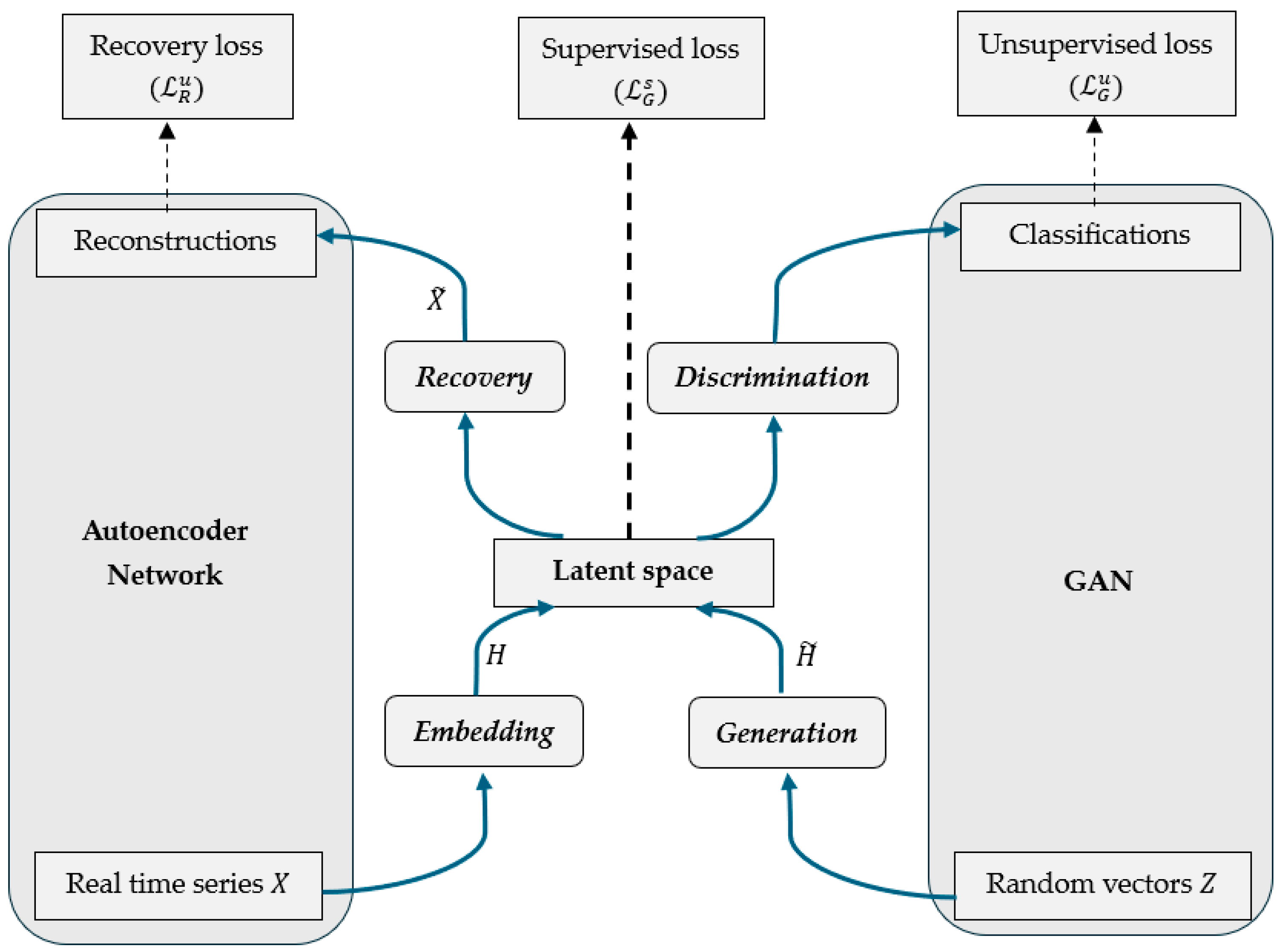
The TGAN architecture comprises four interconnected layers: (i) generator, (ii) discriminator, (iii) embedding network, and (iv) recovery network. Figure 1 illustrates how real carbon price data are embedded, used to generate synthetic sequences, and validated through an adversarial learning process. The TGAN training process combines the standard unsupervised GAN training with an additional supervised learning signal, along with the autoencoder reconstruction objective. All four components (generator, discriminator, embedder, and recovery) are trained together in a multi-task fashion, although in practice, training can be staged for stability (e.g., pre-training the autoencoder). In essence, the two core components of the TGAN model, the generator and the discriminator, operate in a competitive learning process (the typical GAN setup). The generator creates artificial data sequences that mimic real historical patterns, while the discriminator attempts to distinguish between real and synthetic sequences. Through iterative training, the generator learns to produce increasingly realistic time-series data, and the process reaches an equilibrium when the discriminator can no longer differentiate between real and synthetic data. What differentiates TGAN from a standard GAN is its ability to learn complex temporal relationships by incorporating recurrent memory units and an embedding mechanism into the architecture. Moreover, TGAN introduces an autoencoder structure, consisting of an embedding network and a recovery network that works alongside the GAN’s generator and discriminator. The embedding network encodes the original time series into a latent representation (feature space), and the recovery network decodes the generator’s output back to the original data space. By generating data in this latent space, the model ensures that essential temporal features (such as seasonality or slow mean-reverting tendencies) are captured and later reconstructed in the output.

To capture the temporal dependencies and self-correlations inherent in the original time series data, we integrated Long Short-Term Memory (LSTM) layers into the architecture of GAN. LSTM is a type of Recurrent Neural Network known for its capability to remember information over long time lags [64], which is essential for time series like carbon prices that exhibit both short-term fluctuations and long-term trends.

We represent the carbon price series in a matrix format (Equation (6)) to facilitate training the TGAN. If N is the length of the time series and T is the number of time lags considered for each training sample (plus one, to include the current time step), then each row of the matrix corresponds to one sequence of length T extracted from the original series. Each such T-length sequence (each matrix row) serves as a training sample for the LSTM-based generator and discriminator. Prior to training, the time-series values are scaled using a min–max normalizer [65] to ensure stable training.

$$X=\left[\begin{array}{ccccc}{x}_t& x_{t-1}& x_{t-2}& \cdots & x_{t-T}\\ x_{t+1}& x_t& x_{t-1}& \cdots & x_{t+1-T}\\ x_{t+2}& x_{t-1}& x_t& \cdots & x_{t+2-T}\\ & & & \ddots & \\ x_N& x_{N-1}& x_{N-2}& \cdots & x_{N-T}\end{array}\right], X\in \left\{x\in R∣0\le x\le 1\right\}$$

(6)

4.3.2. Training Strategy and Loss Functions

The training strategy and the loss components involved are briefly summarized below. In the autoencoder structure, the embedding network (E acts as an encoder) takes the real carbon price sequence data and compresses it into a latent representation (denoted $H$). This network learns an informative summary of the time series, extracting the essential temporal relationships in a lower-dimensional (or feature-enriched) space. Formally, the embedder maps the original data $X$ to latent features $H$ (Equation (7)), where dimensions $dim\left(H\right)$ can be chosen larger than, equal to, or smaller than the original feature dimension to best capture the dynamics.

$$H=E\left(X\right), H=\left(\begin{array}{c}N\\ T\\ {dim}_H\end{array}\right)$$

(7)

The generator (G) receives input from the latent space and produces synthetic latent sequences. The generator is trained via a joint unsupervised and supervised learning process. In the unsupervised adversarial mode, the generator transforms a random noise tensor $Z$ (Equation (8)) into a synthetic latent sequence $\tilde{H}$ that should resemble latent encodings of real data (Equation (9)). The random noise input $Z$ is not a single vector but a sequence of random vectors of dimension $dim\left(Z\right)$, with the same time length as the training sequences, giving the generator the necessary degrees of freedom to generate sequential patterns. For training, we segment the carbon price series into sequences of length T time steps (e.g., T = 20), forming a training matrix as presented in Equation (6). The unsupervised training is identical to a standard GAN, where the generator tries to produce data that fools the discriminator using the noisy tensor Z as input. Equation (10) represents the generator’s unsupervised loss function (${\mathcal{L}}_G^u$).

$$Z=\left(\begin{array}{c}N\\ T\\ {dim}_Z\end{array}\right), Z_{i,j,k}\sim N\left(0,1\right)$$

(8)

$$\tilde{H}=G\left(Z\right), \tilde{H}=\left({\displaystyle \genfrac{}{}{0pt}{}{N}{T}}\right)$$

(9)

$${\mathcal{L}}_G^u={\displaystyle \frac{\sum _{t=1}^N\log \left(1-D\left(\widetilde{X_t}\right)\right)}{N}}$$

(10)

In contrast, supervised training is realized by generating data from the latent representation obtained by transforming $X$ into $H$ through the embedding network. Specifically, given an embedded real sequence $H$ (where $H_t$ denotes the latent vector at time step t of the real sequence), the generator is asked to predict the next-step latent state. At each time t, using the previous latent state $H_{t-1}$ as input, G produces a predicted latent vector for the current step, denoted $G\left(H_{t-1}\right)$. The LSTM-based generator G then learns to map either random sequences $Z$ or embedded sequences $H$ to synthetic outputs $\tilde{H}$ that follow the patterns of the real data in the latent space. The supervised loss $\left({\mathcal{L}}_G^s\right)$ is then defined as the mean squared error (L2 norm) between the generator’s prediction and the actual embedding $\left(H_t\right)$ at that time step (Equation (11)).

$${\mathcal{L}}_G^s={\displaystyle \frac{\sum _{t=1}^{N-1}{‖H_t-G\left(H_{t-1}\right)‖}^2}{N-1}}$$

(11)

The overall training objective for the generator combines the unsupervised adversarial loss and the supervised loss described above. The objective of the generators’ gradient descent is to minimize $\eta \ast {\mathcal{L}}_G^s+{\mathcal{L}}_G^u$ where the first term $\eta$ controls for the influence of the supervised loss on the training process.

The recovery network (R acts as a decoder) takes the synthetic latent sequence $\tilde{H}$ produced by the generator and reconstructs it back to the original data space, producing a synthetic carbon price sequence $\tilde{X}$ (Equation (12)). This network is the mirror of the embedder and ensures that the generated latent patterns translate into realistic sequences in the original scale and units. The pair of embedding and recovery networks acts as an encoder–decoder (autoencoder), allowing the model to retain temporal structure: any long-term pattern encoded in $H$ should be present in $\tilde{X}$ after reconstruction. Notably, the synthetic data $\tilde{X}$ is not generated directly in the original feature space of $X$, but via this latent space pipeline (embed → generate → recover), which forces the generator to respect the learned structure of real data. The recovery loss is computed by comparing the original vectors with those reconstructed from the generated data. The reconstruction is performed via the recovery network. The overall formulation of the recovery loss is presented in Equation (13).

$$\tilde{X}=R\left(\tilde{H}\right), \tilde{X}=\left({\displaystyle \genfrac{}{}{0pt}{}{N}{T}}\right)$$

(12)

$${\mathcal{L}}_R^u={\displaystyle \frac{\sum _{t=1}^N{‖X_t-\widetilde{X_t}‖}^2}{N-1}}$$

(13)

The adjustment of the embedding and recovery network relies on the supervised loss and the recovery loss. The formula is $\lambda \ast {\mathcal{L}}_G^s+{\mathcal{L}}_R^u,$ where the first term $\lambda$ once again controls the influence of the supervised loss. In the original paper, Yoon et al. [61] observed no overall benefits in reducing the effect of the supervised loss on the two optimizations, prompting us to neglect the existence of $\lambda$ and $\eta$ in our model.

The discriminator (D) develops the ability to distinguish between real and synthetic data, providing adversarial feedback to the generator to improve the quality and realism of the generated sequences (Equation (14)). It outputs a probability D(⋅) representing how likely a given sequence is real.

$$D\left(X\right)\in \left[0,1\right]andD\left(\tilde{X}\right)\in \left[0,1\right]$$

(14)

The model was optimized using the gradient descent of the Binary Cross-Entropy (BCE) loss. Equation (15) is the generalized form of the BCE loss for a single sample where $y$ is the true label of the original data point and $\widehat{y}$ is the predicted probability. Equation (16) illustrates how BCE loss is applied in estimating the discriminator’s loss for an entire batch.

$${\mathcal{L}}_{BCE}\left(y,\widehat{y}\right)=-\left[y·log\left(\widehat{y}\right)+\left(1-y\right)·log\left(1-\widehat{y}\right)\right]$$

(15)

$${\mathcal{L}}_D=-\left({\displaystyle \frac{1}{N}}\right)\ast \sum _{t=1}^N\log \left(D\left(X_t\right)\right)+\log \left(1-D\left(\widetilde{X_t}\right)\right)$$

(16)

By combining these elements, TGAN effectively extends the standard GAN framework to handle chronological properties. During training, the discriminator and generator are trained simultaneously in an adversarial process, leading to an equilibrium where both models are optimized.

4.3.3. Comparative Evaluation and Model Selection

We performed an ablation study to justify the use of TGAN over simpler generative approaches. Specifically, we compared three architectures of increasing complexity: (i) a plain GAN (no embedding network, generator trained only adversarially), (ii) the full TGAN model as described above, and (iii) a variant of TGAN where the standard BCE-based discriminator is replaced by a Wasserstein GAN critic with gradient penalty [63] (a technique often used to stabilize GAN training). All three models were built with the same base architecture (the generator and discriminator each had the same number of LSTM layers and neurons) and were trained on 20-step sequences of the carbon price data for 500 epochs to ensure a fair comparison. To evaluate synthetic data quality, we adopted two evaluation measures inspired by Yoon et al. [61] and other similar studies [66,67].

First, the discriminative test (real vs. synthetic distinguishability), which measures how well an external classifier can distinguish synthetic data from real data. If the synthetic data are very realistic, the classifier should perform no better than random guessing (50% accuracy). We trained a simple one-layer LSTM classifier (with dropout regularization) to classify sequences as “real” or “synthetic”. We then computed its classification accuracy on a held-out set. The discriminative score is defined as the absolute difference |accuracy − 0.5|. An ideal outcome is an accuracy of 50% (score of 0), meaning the classifier cannot tell real from synthetic at all.

Second, the predictive test (train on synthetic, test on real) evaluates the utilitarian quality of the synthetic data—whether models trained on synthetic data can generalize to real data. We trained a predictive model on the synthetic dataset and then tested its performance on real data. Specifically, we used a one-layer LSTM regression model (with dropout) that learns to predict the next time step given the previous 20 steps. We trained this model using synthetic sequences (from each GAN variant) and then evaluated its prediction error on real carbon price sequences (the same task on real data). We report standard forecast error metrics, Mean Absolute Error (MAE), and Mean Squared Error (MSE), for each case. If the synthetic data sufficiently capture the true dynamics, the model trained on synthetic should achieve low error on real data (close to a model trained on real data). Using these metrics, we found that the TGAN-generated data were the most similar to the original data.

4.4. Synthetic Data Validation

To assess the statistical properties of the generated synthetic time series in comparison to the original series, a comprehensive analysis was conducted involving three key steps. (1) The autocorrelation function was calculated for each synthetic time series across various lag values. Key metrics, such as the area under the curve (AUC) and the mean autocorrelation, were extracted to provide insights into the temporal dependencies within each synthetic series. Aggregate statistics were obtained by computing the coefficients for multiple pairs between the synthetic data points and their lagged counterparts. (2) The similarity between the original and synthetic time series was evaluated by computing the cross-correlation between the detrended and deseasonalized original data and the corresponding synthetic data. Positive and negative lag values were considered to capture lead and lag relationships. The AUC and mean cross-correlation values were extracted to quantify the degree of similarity. (3) To further assess the predictive capabilities of the synthetic time series, a two-layer LSTM neural network was trained using an expanding window time-series-split cross-validation approach [68] to predict the residuals of the original time series using synthetic data. The model’s prediction error was evaluated to determine the extent to which the synthetic time series could replicate the dynamic behaviour of the original data.

5. Empirical Results and Discussion

5.1. Descriptive Statistics

This subsection provides a descriptive overview of UK carbon allowance price dynamics between 2022 and 2023. It identifies key patterns of price volatility, seasonal shifts, and the role of regulatory interventions. Particular attention is given to the sharp price decline in 2023, which is linked to verified emissions reductions, increased renewable energy deployment, and announced policy changes affecting allowance supply.

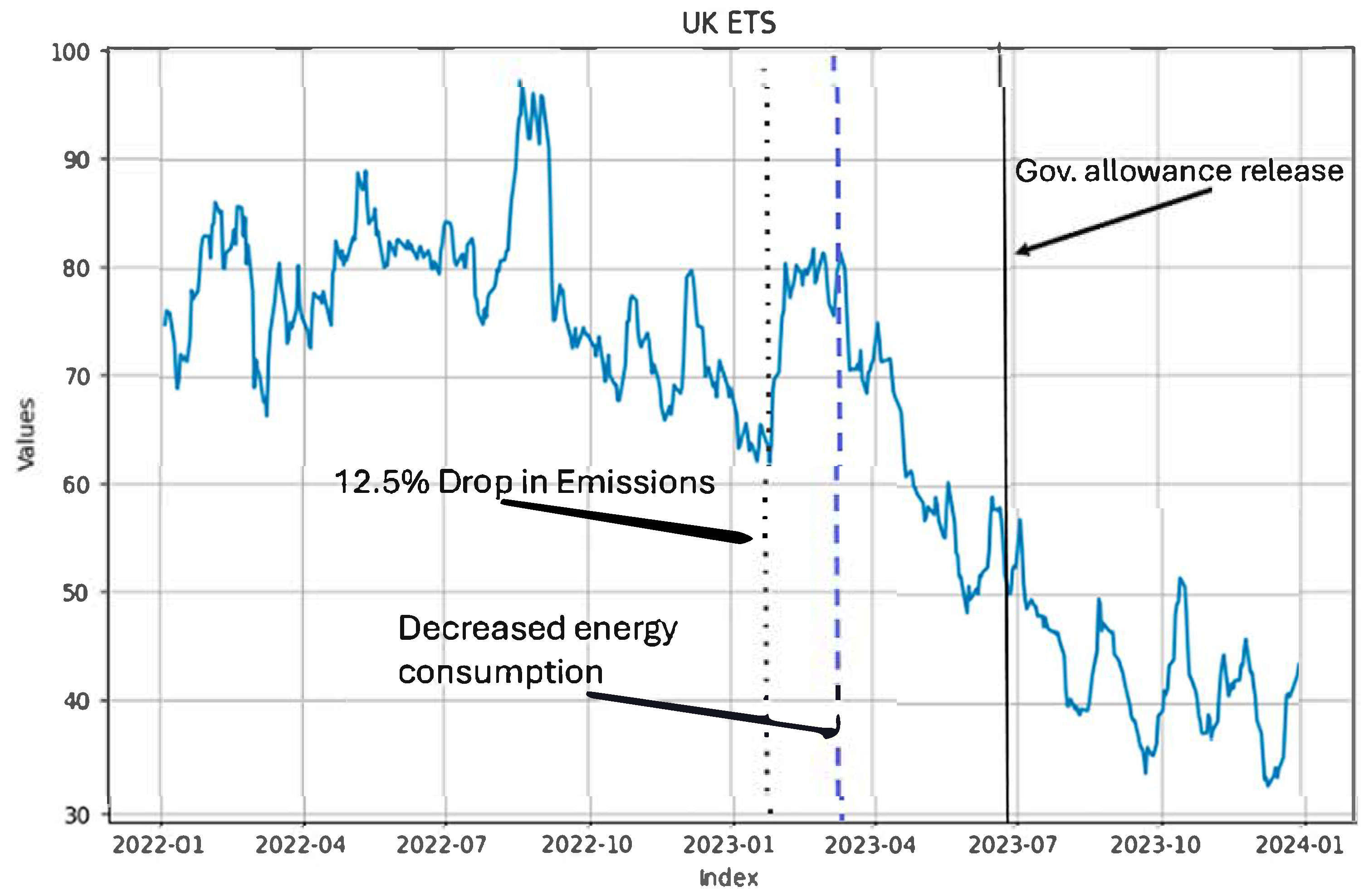
After interpolating the absent time data, the resulting time series exhibits non-monotonic behaviour, characterized by alternating periods of upward and downward trends, as depicted in Figure 2. The figure suggests that the UK ETS market experienced significant price volatility in 2022, reaching peak levels before entering a prolonged downward trend throughout 2023, consistent with market uncertainties and fluctuations in supply-demand dynamics. The observed decline in UK ETS allowance prices during 2023 can be attributed to several key factors. One major factor influencing this decline was verified emissions under the UK ETS, which fell by 12.5% in early 2023, largely due to an accelerated shift from fossil fuels to renewable energy sources in electricity generation [69]. This decline in emissions reduced the demand for carbon allowances, aligning with the start of a sustained downward trend, reinforcing the connection between reduced emissions and lower demand for allowances.

Additionally, in the first and second quarters of 2023, the UK experienced a decline in its carbon-intensive energy consumption and an increase in its renewable energy generation. For example, in the first quarter of 2023, gas demand was 6.1% lower than gas demand in the same quarter of the previous year, whereas renewables’ share of total electricity generation reached a record high of 47.8% [70]. These combined factors reduced the need for carbon-intensive energy production companies to purchase ETS allowances, lowering prices during March and April 2023. Moreover, the UK government’s announcement in July 2023 regarding the release of an additional 53.5 million carbon allowances between 2024 and 2027. These allowances, originally unused from 2021 to 2023, created a market perception of oversupply, accelerating the price decline. Thus, the observed price behaviour in Figure 2 aligns with market fundamentals, where both regulatory actions (such as allowance releases) and structural changes (such as emissions reductions) played a significant role in shaping UK ETS price trends.

The descriptive statistics of the time series in

Table 2. UK ETS descriptive statistics (2022–2023).

Statistic	Value	Statistic	Value
Basic Statistics		Temporal Statistics
Mean	65.91	Mean of First Difference	−0.06
Median	71.08	Std Dev of First Difference	1.77
Mode	79.95	Mean of 30-day Rolling Means	66.44
Range	64.59	Std Dev of 30-day Rolling Means	15.46
Variance	270.01	Mean of 90-day Rolling Means	67.44
Standard Deviation	16.43	Std Dev of 90-day Rolling Means	13.85
Interquartile Range (IQR)	29.62	Mean Percentage Change
Skewness	−0.48	30-day Windows	−0.025
Kurtosis	−1.03	90-day Windows	−0.066
		Extremes
		Minimum Value	32.56
		Maximum Value	97.15

Source: Authors’ calculations.

indicate that the UK ETS market exhibited significant price fluctuations between 2022 and 2023, as reflected in a wide price range and a high standard deviation, suggesting notable variability in allowance prices. The market also showed a marginal negative average price change daily, as indicated by the mean of the first difference, with daily changes displaying noticeable dispersion. Over 30 days, the average percentage change was slightly negative, suggesting a minimal price decrease. Similarly, the 90-day average percentage change indicates a stronger downward trend over a longer horizon. While the overall price level fluctuated, the 30-day and 90-day rolling means remained slightly higher than the average, suggesting a slight upward trend in average prices. However, the negative average percentage change suggests that despite the slight increase in rolling means, the overall trend in carbon prices remained downward.

5.2. Time Series Decomposition

This subsection investigates the underlying trend and seasonal structures of the carbon price series using polynomial regression, Fourier-based models, and LOESS decomposition. The goal is to isolate deterministic components from the time series and assess whether residual structures exhibit long-range dependencies. Emphasis is placed on comparing monthly (30-day) and quarterly (90-day) seasonality and interpreting the implications of the residual dynamics.

In order to gain deeper insights into trends and seasonal behaviours of the data, Simple Linear Regression (SLR), Polynomial Regression, and Fourier Transform Regression models are applied. Two modelling approaches were investigated: (i) Sequential (SQ) and (ii) Mixed (MM). The obvious difference lies in the more rigid structure of SQ that effectively isolates the trend component from the seasonal component. This distinction in the modelling approach is reflected in the regression statistics presented in

Table 3. Statistics of linear regressions.

	SLR	2nd°	3rd°	4th°	5th°	6th°
Akaike Information Criterion (AIC)	3083.246	4753.883	4692.984	4659.282	4636.032	6628.589
Bayesian Information Criterion (BIC)	3074.074	4740.124	4674.640	4636.351	4608.515	6605.659
Shapiro–Wilk (SW) p-values	0.000	0.000	0.000	0.000	0.000	0.000
R2	0.743	0.851	0.864	0.871	0.877	−0.945

Source: Authors’ calculations.

and

Table 4. Statistics of combined linear and Fourier Transformed Regressions.

	SQ1	SQ2	SQ3	SQ4	MM1	MM2	MM3
AIC	3079.808	3056.349	2553.483	2515.283	5135.269	5108.523	4643.058
BIC	3102.739	3088.452	2590.172	2579.489	5153.614	5126.868	4670.575
Fourier R2	0.001	0.038	0.002	0.069	-	-	-
R2	-	-	-	-	0.743	0.753	0.871
SW p-values	0.000	0.000	0.000	0.000	0.000	0.000	0.000
Harmonic Order	1	1	2	4	1	1	1
Polynomial Degree	SLR	SLR	5	5	SLR	SLR	3
Period Length	30	90	30	90	30	90	90

Source: Authors’ calculations.

.

The polynomial regression models in Table 3 demonstrate increasing R² values from Simple Linear Regression up to the fifth degree, suggesting improved fit with added complexity. However, the sixth-degree model exhibits severe overfitting, evidenced by a negative R² and drastically higher AIC/BIC values, indicating instability. While the fifth-degree polynomial achieves the highest R², the fourth-degree model is preferable due to its lower AIC and BIC, presenting a better balance between fit and parsimony.

In Table 4, the low Fourier R² values for the SQ models suggest a limited ability to capture seasonal patterns. MM models generally perform well in trend modelling, with MM3 achieving the highest R² (0.8706), comparable to the best linear models. While Simple Linear Regression initially exhibits better AIC/BIC values than polynomial models, this trend reverses when combined with seasonal regression. The fifth-degree polynomial model produces the best coefficient estimates, suggesting that it provides the most accurate representation of the underlying trend and seasonal patterns in the data. Notably, SQ1 and MM1 include insignificant coefficients in their sinusoidal terms, suggesting that 90-day periods explain the periodic pattern much better than the 30-day periods. MM3 is the only mixed model approaching the goodness of fit of the fifth degree, although it performs better in terms of AIC, BIC, and score when compared to the equivalent 3rd-degree polynomial model, having a lower value in all of them. Finally, Shapiro–Wilk tests reveal non-normality in the residuals of all models, implying that even after accounting for trend and seasonality, the time series may still possess non-Gaussian properties indicative of long-term dependence. These results motivate further investigation into the underlying patterns, which can yield a deeper understanding of the price properties of carbon allowances if the trend and seasonality are removed.

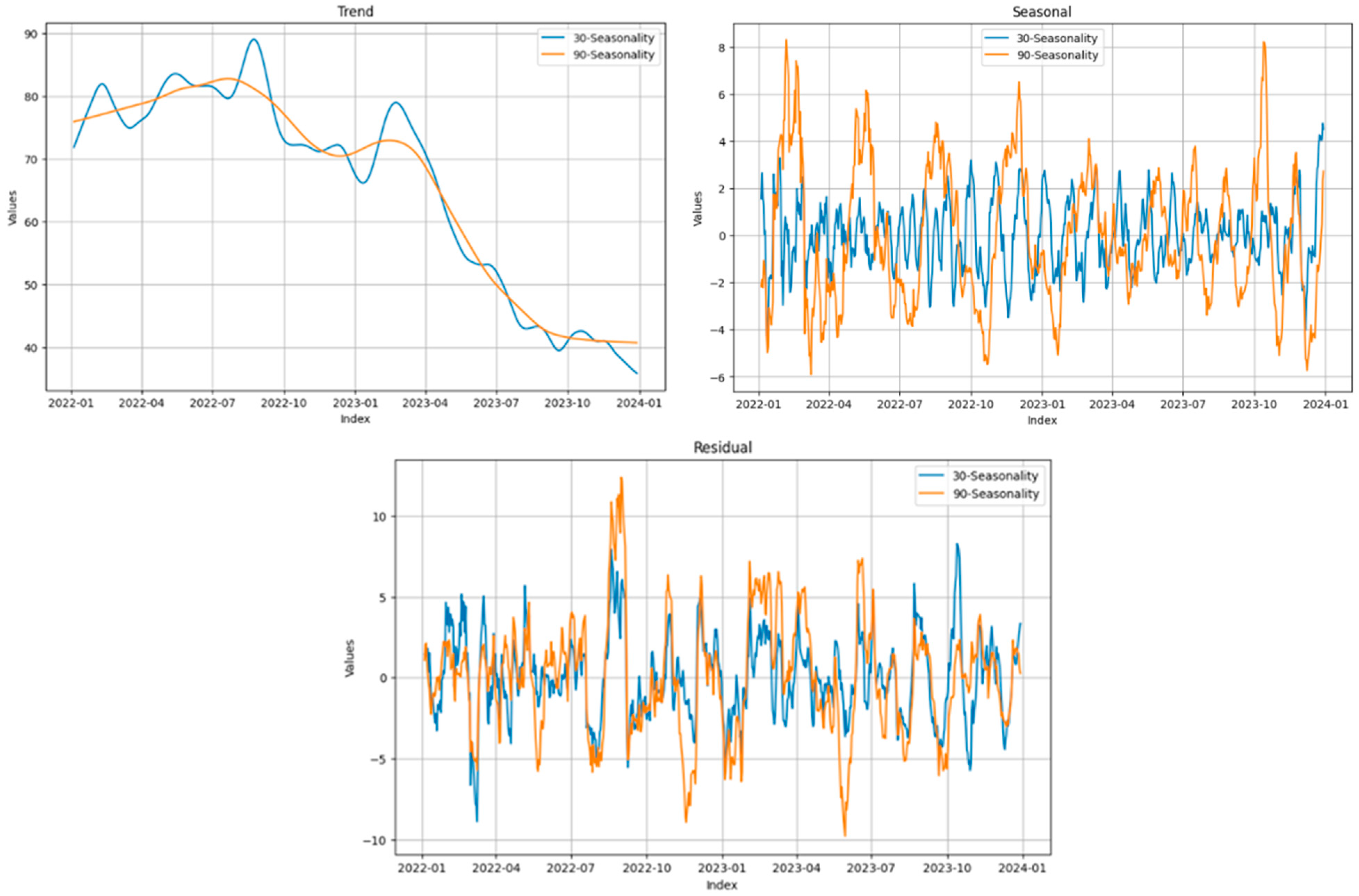
LOESS decomposition was employed to separate the time series into three components: trend, seasonality, and residuals. This analysis helps in understanding both the systematic trends and the cyclical behaviours present in the data, supporting more informed forecasting and decision making. The decomposition results are presented in Figure 3, comparing 30-day (monthly) and 90-day (quarterly) seasonal effects. The trend shows a significant long-term decline, especially from early 2023 onward. Seasonal effects differ between monthly and quarterly models, with the monthly model capturing more frequent fluctuations and the quarterly model highlighting broader cycles. Residuals suggest that while most patterns are explained, some unpredictable behaviours remain, potentially due to market shocks or policy changes.

To facilitate the discussion, the residuals from the monthly and quarterly decompositions are referred to as M-SEAS (monthly seasonal decompositions) and Q-SEAS (quarterly seasonal decompositions), respectively.

Table 5. Time series statistics.

Time Series	ADF Statistic	p-Value	Shapiro Statistic	p-Value	Hurst Parameter
Monthly Season	−7.477	0.000	0.997	0.232	0.566
Quarterly Season	−6.503	0.000	0.989	0.000	0.758

Source: Authors’ calculations.

demonstrates that the properties of the residuals vary depending on the selected seasonal configuration. A Shapiro–Wilk test at a significance level of 0.05 indicates that the residuals from the monthly decomposition are approximately normally distributed, exhibiting behaviour similar to random Gaussian noise. In contrast, the residuals from the quarterly decomposition are non-normally distributed, suggesting that the time series may possess characteristics beyond those captured by seasonality and trend. Both M-SEAS and Q-SEAS are confirmed to be stationary based on the results of the Augmented Dickey–Fuller (ADF) test, confirming their suitability for time series modelling. The Hurst parameter for both series was estimated using Rescaled Range (R/S) analysis. As expected, M-SEAS, which fails to differ substantially from random noise, has a Hurst parameter close to 0.5, indicating near-random behaviour with minimal persistence. In contrast, Q-SEAS displays clear long-memory behaviour, suggesting that past trends are likely to persist or recur over time.

5.3. Configuring the Synthetic Data Generation Through the Deep Learning Model

This subsection focuses on configuring the TGAN model for optimal synthetic data generation. An ablation study is conducted to compare three generative architectures, with performance evaluated across both monthly and quarterly residuals. Bayesian optimization is applied to tune hyperparameters, and model complexity is adjusted to reflect the statistical properties of the input series—particularly the persistence of long-memory structures in the quarterly decomposition. WTGAN refers to a Wasserstein-based adaptation of TGAN, designed to improve convergence stability by minimizing the Wasserstein distance between real and synthetic time-series distributions.

For determining the best GAN architecture through the ablative analysis, we have used both the Q-SEAS and the M-SEAS datasets, showcasing the study’s results in

Table 6. Ablation study.

Iteration	Method	Discriminative (Absolute Accuracy)	Predictive (MSE)
M–SEAS	GAN	0.0203	6.755414
Q–SEAS		0.0483	3.68814
M–SEAS	TGAN	0.0372	1.23505
Q–SEAS		0.0913	0.847832
M–SEAS	WTGAN	0.0417	1.702863
Q–SEAS		0.0637	1.78071

. As mentioned, the TGAN displays the greatest ability to replicate the original data.

Hyperparameter tuning is a required step in any quantitative analysis that employs complex neural networks. From among the traditional methods, we had the option of adopting either grid search or random search, both having the advantage of being fairly simple to implement. The lack of heuristic reasoning is cited as the main limitation of this method [71,72], and the method appears to underperform in comparison to Bayesian Search, Genetic Algorithms, or other task-specialized optimization methods [71,72,73,74]. Grid Search, while considered the most widely used, was noted on the other hand to be a poor choice for high-dimensional hyperparameters due to the high computational cost, suitable instead for 1D or 2D hyperparameters [74]. Grid Search was found to underperform, for example, Bayesian Search in comparison tests [75]. To simplify the optimization process, we have decided to fix the learning rates for the embedding and recovery networks at 10⁻⁴ and tune only the learning rates for the generator and discriminator and the size of batches used for training the TGAN on the M-SEAS and Q-SEAS time series using a simple Bayesian Search. The number of lags was heuristically decided using the Autocorrelation Function (ACF) and the Partial Autocorrelation Function (PACF) as guidance. For the initiation of the Gaussian Process, we used we generated 10 hyperparameters by randomly sampling from a uniform distribution values bounded between 10⁻² and 10⁻⁵ for the learning rate and 10 to 100 for the batch size. We updated the Gaussian Process another 20 times until we obtained a matrix of 30 different hyperparameter combinations. The objective function used for this search algorithm was the distance between the Hurst Parameter of the real dataset and that of the generated data. After fitting the Gaussian Process on the updated hyperparameter matrix, we select the hyperparameter configuration with the highest mean performance (exploitation). For simplicity, we round the learning rates afterwards to the closest power of 10 and the batch size to the closest multiple of 10.

5.4. Synthetic Data Generation, Validation, and Comparison

This subsection presents a comparative evaluation of three synthetic data generation methods—fBm, adjusted fBm, and TGAN—based on their ability to replicate key statistical and predictive properties of the original series. The analysis includes autocorrelation and cross-correlation diagnostics, as well as LSTM-based out-of-sample testing. Findings highlight that while all synthetic models outperform standard Brownian motion, adjusted fBm and TGAN offer distinct advantages depending on the validation metric used.

Three types of synthetic time series, each matching the length of the original time series, were generated. The fBm dataset, produced solely through fractional Brownian motion, models long-term memory and self-similarity. The Adjusted fBm dataset, created by applying spectral decomposition to the fBm, captures the specific variance patterns of the original time series. The TGAN dataset, generated using a TGAN neural network, is a deep learning model designed to replicate the statistical properties of the original time series. The Area Under the Curve (AUC) and mean correlation values offer insights into the overall correlation strength between the synthetic and original time series.

Subsequently, for each of the three data generation methods, three sets of synthesized datasets were produced and compared to the original time series. For each iteration, cross-correlation and autocorrelation analyses were conducted to evaluate self-similarity and similarity to the historical data. Various hyperparameter configurations were tested, and the properties of the simulated synthetic data were analyzed. The configuration in

Table 7. Model configuration.

Properties/Hyperparameters	M-SEAS	Q-SEAS
Generator Learning Rate (LR)	Adaptive Moment Estimation (ADAM) 10−3
Discriminator Learning Rate (LR)	Adaptive Moment Estimation (ADAM) 10−4
Embeddings Learning Rate (LR)	Adaptive Moment Estimation (ADAM) 10−4
Generator Structure	1× Perceptron Layer—64 Neurons 1× LSTM Layer—64 Neurons 2× Dropout Layers—10% Output Layer—Sigmoid Activation
Discriminator Structure	1× LSTM Layer—64 Neurons 1× Perceptron Layer—64 Neurons 2× Dropout Layers—10% Output Layer—Sigmoid Activation
Embedding Structure	1× LSTM Layer—64 Neurons 1× Perceptron Layer—64 Neurons—Relu Activation 2× Dropout Layers—10%
Recovery Structure	1× LSTM—64 Neurons
Lags	20 Consecutive Lags	50 Consecutive Lags
Noise Dimension	5	5
Batches	50	100
Epochs	1000	1400
Loss Function	Binary Cross Entropy
Hurst Iteration 1	0.603	0.721
Hurst Iteration 2	0.574	0.782
Hurst Iteration 3	0.577	0.822

Source: Authors’ calculations.

was identified as the most effective for generating synthetic data that closely mirrors the original series’ properties. The models successfully produced stationary data, as indicated by the ADF test, and captured long-term dependencies, as shown by the Hurst parameter. While the M-SEAS model effectively models short-term dependencies with behaviour similar to Gaussian noise, the Q-SEAS model captures strong long-term persistence, a requirement for modelling time series with memory effects. The higher training iterations in the Q-SEAS model are justified by the desire to capture the more persistent patterns suspected to exist in the Q-SEAS data compared to the M-SEAS data. Overall, the optimized configurations enable the generation of realistic synthetic data, supporting robust modelling and simulation of the original time series.

As discussed earlier, M-SEAS is expected to contain minimal additional information beyond what was captured in the trend and seasonal components.

Table 8. M-SEAS synthetic data (20 lags).

Iteration	Method	Mean Correlation (Auto)	AUC (Auto)	Mean Correlation (Cross)	AUC (Cross)
1	TGAN	0.099	2.206	−0.011	2.223
2		0.070	1.962	−0.015	0.992
3		0.060	1.712	−0.012	1.316
1	fBm	0.970	20.365	−0.019	0.764
2		0.903	18.969	0.017	0.832
3		0.877	18.422	−0.038	1.739
1	Adjusted fBm	0.507	10.643	−0.066	3.234
2		0.422	9.924	0.026	4.668
3		0.358	10.229	−0.023	5.270

Source: Authors’ calculations.

presents the properties of the synthetic data generated for M-SEAS. The mean autocorrelation is highest for fBm and lowest for TGAN, indicating that the fBm model better preserves autoregressive patterns than TGAN. The AUC values support this trend, where fBm consistently outperforms the other two models. While all three models struggle to fully capture the characteristics of the original time series, as evidenced by the mean cross-correlation, the Adjusted fBm appears to perform slightly better based on its AUC value. Based on these findings, we conclude that for M-SEAS, the pure fBm model is most effective in preserving autocorrelation characteristics.

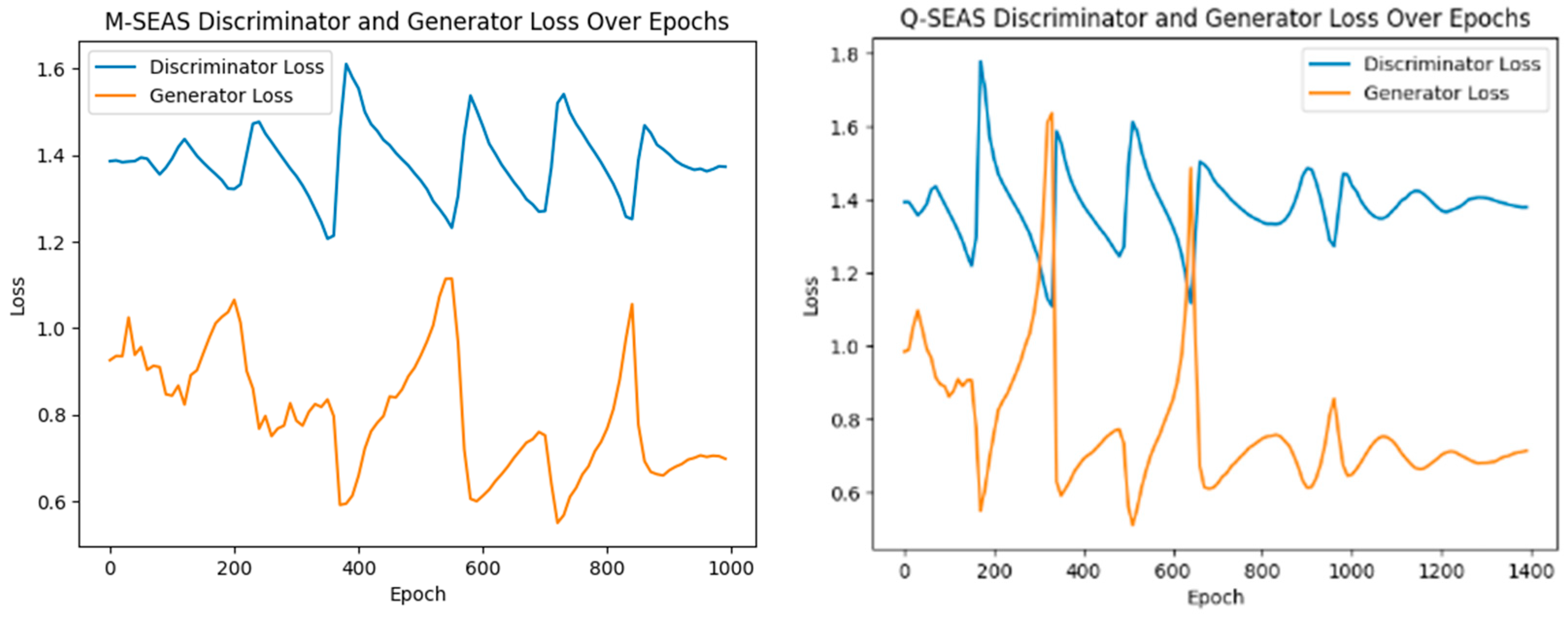
Figure 4 illustrates the learning process of the TGAN network. As observed, the discriminator and generator gradients oscillate inversely. As the networks continue to update, these oscillations diminish, indicating that the model converges toward an optimal state during later epochs. The generator loss in both cases is also lower than it started, which is another good sign that the model has improved its replicating capabilities. It still must be noted that the neural networks appear to struggle to achieve a balance and understand the properties of the data, a common challenge in training GANs, hinting that the model architecture can be further improved to achieve higher stability.

For the Q-SEAS series, the TGAN model again exhibited the lowest autocorrelation and cross-correlation values (as indicated in

Table 9. Q-SEAS synthetic data (50 lags).

Iteration	Method	Mean Correlation (Auto)	AUC (Auto)	Mean Correlation (Cross)	AUC (Cross)
1	TGAN	0.089	4.631	0.006	2.814
2		0.105	5.520	−0.004	2.343
3		0.156	7.958	−0.005	2.957
1	fBm	0.872	44.494	−0.041	4.176
2		0.599	30.543	0.162	16.422
3		0.733	37.404	−0.010	3.379
1	Adjusted fBm	0.659	33.603	0.024	6.113
2		0.557	28.406	0.165	17.352
3		0.497	25.322	−0.073	9.789

Source: Authors’ calculations.

), showing a poor ability to capture the long-term properties of the original residuals. While fBm achieved stronger autocorrelation, its cross-correlation with the original data were inconsistent. In contrast, the Adjusted fBm demonstrated moderate autocorrelation and the strongest, most consistent cross-correlation with the original data. Overall, the Adjusted fBm model demonstrated the most balanced performance, effectively capturing short-term and long-term dependencies in the original time series.

Table 10. M-SEAS regression results (20 lags).

Step	TGAN		fBm		Adjusted fBm		BM
	Loss	MAE	Loss	MAE	Loss	MAE	Loss	MAE
F1	4508.031	66.796	779.597	23.289	3502.968	54.327	3574.500	58.674
F2	196.430	11.288	87.622	7.774	121.573	9.298	113.845	8.870
F3	92.865	7.417	38.385	4.980	69.259	6.294	24.449	3.976
F4	94.377	7.773	62.707	5.981	78.992	6.832	55.099	5.920
F5	48.901	5.126	42.838	5.017	28.042	4.073	41.008	4.987
Average	988.121	19.680	202.230	9.408	760.167	16.165	735.550	16.361
Test MAE	-	31.717	-	66.868	-	28.276	-	168.457
ARIMAX	-	8.509	-	-	-	-	-	-
p-value	-	0.000	-	0.000	-	0.000	-	0.000

Source: Authors’ calculations.

and

Table 11. Q-SEAS regression results (50 lags).

Step	TGAN		fBm		Adjusted fBm		BM
	Loss	MAE	Loss	MAE	Loss	MAE	Loss	MAE
F1	4962.962	70.344	5332.580	72.929	1167.429	28.501	3129.717	51.720
F2	5993.598	77.270	1425.070	32.994	1669.346	29.966	3641.662	59.421
F3	6111.878	78.065	633.229	21.168	4506.069	62.905	5497.762	70.583
F4	283.439	12.612	39.717	4.892	4586.618	66.084	8370.829	83.445
F5	63.396	6.191	6166.841	78.259	6123.028	77.976	858.118	20.696
Average	3483.055	48.897	2719.487	42.048	3610.498	53.086	4299.618	57.173
Test MAE	-	38.395	-	42.002	-	72,305.797	-	113.539
ARIMAX	-	8.567	-	-	-	-	-	-
p-value	-	0.000	-	0.000	-	0.000	-	0.000

Source: Authors’ calculations.

present the results of the LSTM regression network trained to evaluate the predictive capabilities of the generated time series for M-SEAS and Q-SEAS. A fourth synthetic time series, generated using a standard Brownian Motion (BM) process, was introduced as a baseline. The dataset was partitioned into 50% for training, 10% for validation, and 40% for testing, with each segment maintaining the original order of the data points. A 5-fold time-split cross-validation approach was applied for model training. The model architecture consists of two LSTM layers: the first with 50 neurons and the second with 30 neurons, both employing the Rectified Linear Unit (ReLU) transformation, followed by a final output perceptron. Dropout and regularization were implemented between layers, randomly omitting 20% of data points to mitigate overfitting.

For M-SEAS, the TGAN produced the second-highest loss and Mean Absolute Error (MAE) averaged across training folds, indicating inferior performance relative to fBm. In contrast, the fBm model demonstrated the best training performance. However, during testing, the fBm model exhibited signs of overfitting, implying that TGAN may generalize more effectively. Overall, the TGAN outperformed both the standard fBm and Adjusted fBm models in testing. In the case of M-SEAS, all synthetic time series outperformed BM in predicting the original series, indicating the presence of predictive power in the generated data.

The regression results for Q-SEAS (presented in Table 11) provide insights into the learning process and the predictive capabilities of the synthetic data. TGAN exhibited the lowest average MAE and loss across all but the fourth fold. On average, fBm achieved the second lowest MAE during training, while the Adjusted fBm showed mixed results during training. During the testing phase, TGAN had the lowest MAE, suggesting a superior ability to predict out-of-sample data. Conversely, Adjusted fBm exhibited the worst MAE, indicating model instability. Overall, in the case of Q-SEAS, all three synthetic data series outperformed the BM, indicating that the original time series exhibits latent structures and long-memory behaviour.

Given that the proposed validation framework involves training an LSTM model on synthetic time series and evaluating it on the original data, it cannot be directly compared to the ARIMAX model due to fundamental methodological differences in their structure and data inputs. Nonetheless, ARIMAX is included as an auxiliary reference to contextualize model performance. To complement this, a multiple linear regression (MLR) model was also applied to the same datasets, with results reported in Table 10 and Table 11. Notably, ARIMAX yields the lowest mean absolute error in both Table 10 (MAE = 8.509) and Table 11 (MAE = 8.567), with statistically significant results (p = 0.000), underscoring its high predictive accuracy. However, these outcomes are not intended as direct benchmarks for the LSTM-based architecture due to the fundamental differences in data handling and model structure. While ARIMAX is trained directly on the original series, the LSTM model operates on sequences derived from synthetic data. Therefore, ARIMAX serves strictly as a contextual anchor, illustrating the potential performance of classical models and emphasizing the need for benchmarking approaches that are methodologically aligned with the validation strategy employed.

5.5. Model Robustness and Validation

This subsection evaluates the robustness and generalization capacity of the proposed deep learning models, with a particular focus on mitigating overfitting risks. Given the complexity and flexibility of architectures such as TGAN and adjusted fBm, we implement a multi-layered validation strategy—including expanding window cross-validation, Bayesian hyperparameter optimization, and dropout regularization—to simulate realistic forecasting conditions and assess model stability across different temporal regimes.

Given the complexity and flexibility of hybrid deep learning architectures, a key methodological concern is ensuring that observed forecasting performance is not the result of model overfitting or data leakage. The risks associated with overfitting are particularly relevant in real-world applications, where models may learn patterns specific to a historical dataset but fail under new or irregular market conditions. In the context of carbon markets, this can lead to inaccurate risk assessments or trading strategies that no longer hold in practice. To address these risks, it is essential to implement rigorous validation techniques. This section outlines the validation strategies adopted to assess the robustness and generalization capacity of the proposed modelling framework, particularly the Time-series Generative Adversarial Network (TGAN) and adjusted fractional Brownian motion (fBm) models.

A multi-layered validation protocol was employed to simulate real-world forecasting conditions and evaluate model stability across different data regimes. Specifically, a time-series cross-validation procedure based on an expanding window approach was used to generate successive training and test sets without compromising temporal causality. This method is particularly well-suited for financial and energy time series, where standard K-fold cross-validation may introduce look-ahead bias.

Moreover, Bayesian optimization was applied to fine-tune hyperparameters for the TGAN’s ability to recreate data that preserve the LTD characteristics of the training data. The optimization criterion was based on the difference between the estimated Hurst parameter of the real residual data and the generated data. To avoid overfitting in deep learning components, techniques such as dropout and regularization were also applied.

The empirical robustness of the models is demonstrated in Section 5.4, which reports performance metrics across both in-sample and out-of-sample evaluation windows. The TGAN model shows consistently superior performance compared to fBm and Brownian motion baselines, especially on the Q-SEAS dataset. These findings demonstrate that the model does not merely overfit the training data. Instead, it effectively captures underlying structural patterns that generalize to future, previously unseen observations.

The validation strategies implemented confirm that the hybrid models are suitable for reproducing the long-term dependence patterns necessary for real-time forecasting in emerging carbon markets. This is particularly relevant in contexts such as the UK ETS, where price dynamics are affected by both structural policy shifts and short-term volatility. The ability of the models to generalize beyond the training regime suggests that they can be reliably integrated into forecasting tools or early-warning systems used by market analysts and regulatory bodies.

While the current robustness checks indicate a certain level of reliability within the UK ETS context, future work should extend these tests across multiple ETS regimes (e.g., EU ETS, California Cap-and-Trade) and under different market phases (e.g., during external shocks or regulatory transitions). Additionally, regime-switching validation frameworks or adversarial robustness tests could further reinforce the empirical stability of hybrid models in high-stakes policy applications.

6. Conclusions and Implications

This study integrates advanced computational methods, including deep learning and statistical modelling, to analyze and simulate the price behaviour of the UK Allowance Futures Contract (UKAFMc1). By applying Simple Linear Regression (SLR), Polynomial Regression, and Fourier Transform Regression, it effectively models the underlying trends and seasonality in carbon market prices using Sequential (SQ) and Mixed (MM) modelling approaches. While some models, including MM3, achieved high R², the regression residuals retained possible unaccounted properties. The combination of polynomial regression with Fourier-based seasonal adjustments showed that fifth-degree polynomial models offered the best fit. Moreover, the 90-day seasonality better explained the periodic behaviour than the 30-day cycle. LOESS decomposition further highlighted a significant long-term shift in carbon prices, characterized by an initial growth followed by a general downward trend from early 2023 onward. The monthly decomposition (M-SEAS) effectively modelled short-term fluctuations, leaving mostly random noise in the residuals. In contrast, the quarterly decomposition (Q-SEAS) revealed long-term persistence and deeper underlying patterns, as confirmed by a high Hurst parameter, indicating that future models must account for long-term dependencies.

To further explore these dynamics, synthetic time series were generated using fractional Brownian motion (fBm), Adjusted fBm (enhanced with the autocovariance matrix), and Time-series Generative Adversarial Network (TGAN). Comparative analysis revealed that the Adjusted fBm consistently outperformed fBm and TGAN in preserving autocorrelation and cross-correlation properties. However, Adjusted fBm exhibited overfitting during testing, raising concerns about its generalization capabilities. Nevertheless, all synthetic models, including fBm, Adjusted fBm, and TGAN, outperformed random noise—the baseline Brownian motion—confirming the existence of self-similar patterns in UK Carbon Permits and supporting the first hypothesis. To contextualize the performance of the proposed models, we also included an ARIMAX model as a traditional reference while acknowledging the architectural and functional differences between approaches. This provides an additional benchmark, suggesting that synthetic data-driven and neural network-based methods can achieve competitive performance in carbon price forecasting. These findings suggest that the models effectively capture some inherent structures in the data, even if not perfectly. These results are consistent with previous research, reinforcing the presence of long-term memory characteristics in financial time series [76]. Unlike prior studies, which primarily focused on general asset markets, this research applies these methodologies to UK Carbon Permits, demonstrating their relevance in an emissions trading context. This domain-specific validation enhances the robustness of existing models while providing practical implications for policymakers and market participants.

The second hypothesis that concerns the models’ ability to capture long-term dependencies fully remains inconclusive due to TGAN’s poor correlation with the original data. However, TGAN demonstrated superior out-of-sample predictive performance, particularly for Q-SEAS. This outcome aligns with findings from [77]. Additionally, research on China’s Hubei and Guangdong carbon markets by [78] highlighted GANs’ ability to leverage multi-source information and extract time-series features, enhancing their performance in modelling carbon price fluctuations. Moreover, using TGAN for data augmentation in the EU Emissions Trading System (ETS) Phase 4 improved prediction accuracy by generating expanded datasets, which enhanced the training process [79]. Although TGAN exhibited poor correlation with the original data, its strong out-of-sample performance suggests potential for further improvement. Addressing these limitations requires refining the GAN architecture and hyperparameters to enhance model stability and better replicate the statistical properties of the original data.

This study offers key economic implications for carbon market participants, policymakers, and financial institutions. The observed long-range dependence in carbon prices suggests that price movements are not purely random but are influenced by historical price trends and regulatory interventions rather than purely current market conditions. This finding aligns with research that challenges the Efficient Market Hypothesis in carbon trading, as price signals may not always align with fundamental abatement costs. This directly affects market efficiency, as predictable structures may allow investors to develop data-driven trading strategies, which have implications for speculative trading and market stability. Since the UK ETS deviates from strong market efficiency, regulatory actions and market expectations of future interventions introduce distortions, potentially affecting investment decisions. To mitigate such risks, the superior predictive performance of models like TGAN and Adjusted fBm suggests strong potential for algorithmic trading applications, provided safeguards are in place to monitor model-driven market dynamics.

Based on the findings and model evaluations, the following time-bound policy recommendations are proposed to enhance the performance, transparency, and resilience of the UK ETS market. In the short term, it is recommended to establish a transparent allowance release calendar that aligns with emission projections and prevailing market conditions. This would help reduce market volatility and discourage speculative trading behaviour. A dynamic price collar—setting a flexible minimum and maximum price range—should be introduced and adjusted semi-annually to prevent excessive price fluctuations while maintaining the integrity of market-based price discovery mechanisms. Additionally, quarterly policy outlooks should be published, including projected intervention thresholds, emissions trends, and key market risk indicators, to enhance transparency and build market confidence.

Over the medium term, the reintroduction or adaptation of a UK-specific Market Stability Reserve (MSR) is recommended. This mechanism should be informed by long-memory indicators and regime-switch detection methods, such as those discussed in Section 5.2 and Section 5.4, to allow for dynamic management of certificate supply in response to market signals. Furthermore, regulatory bodies should pilot the adoption of AI-based monitoring tools, leveraging advanced deep learning models like TGAN and fractional Brownian motion (fBm) for early warning systems. These tools would be instrumental in detecting structural shifts or emerging instabilities in price behaviour.

Looking ahead, partial interoperability with the EU Emissions Trading System (EU ETS) should be pursued. This integration would enhance market liquidity and reduce arbitrage-induced volatility, as supported by the autocorrelation analyses presented in the study. Additionally, the incorporation of forecasting models with long-memory structures into regulatory planning and carbon budget simulations is essential. Such integration would ensure that short-term volatility management is effectively aligned with long-term decarbonization goals. The implementation of these policy measures would significantly enhance the operational efficiency and stability of the UK Emissions Trading Scheme (UK ETS), while promoting a forward-looking, data-informed regulatory approach to carbon market governance.

This study contributes to the understanding of carbon price dynamics by linking empirical evidence from the UK ETS with established economic theory on carbon pricing mechanisms. The findings highlight that cap-and-trade markets exhibit more complex price behaviours than traditional economic models predict, with long-memory effects and regulatory sensitivity playing key roles in price fluctuations. This research provides a stronger foundation for designing more effective carbon pricing policies, ensuring that market mechanisms remain efficient in driving emissions reductions and fostering low-carbon investments.