

Quantum Creation of a Friedmann-Robertson-Walker Universe: Riesz Fractional Derivative Applied


Abstract
1. Introduction
2. Fractional WKB Tunneling Probabilites
3. Results
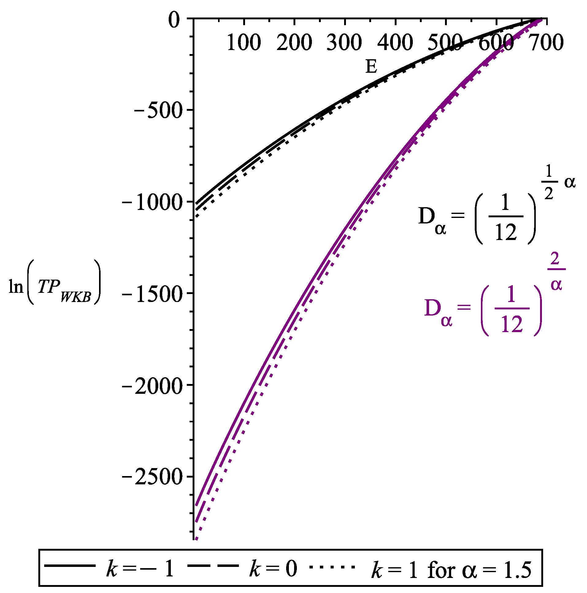
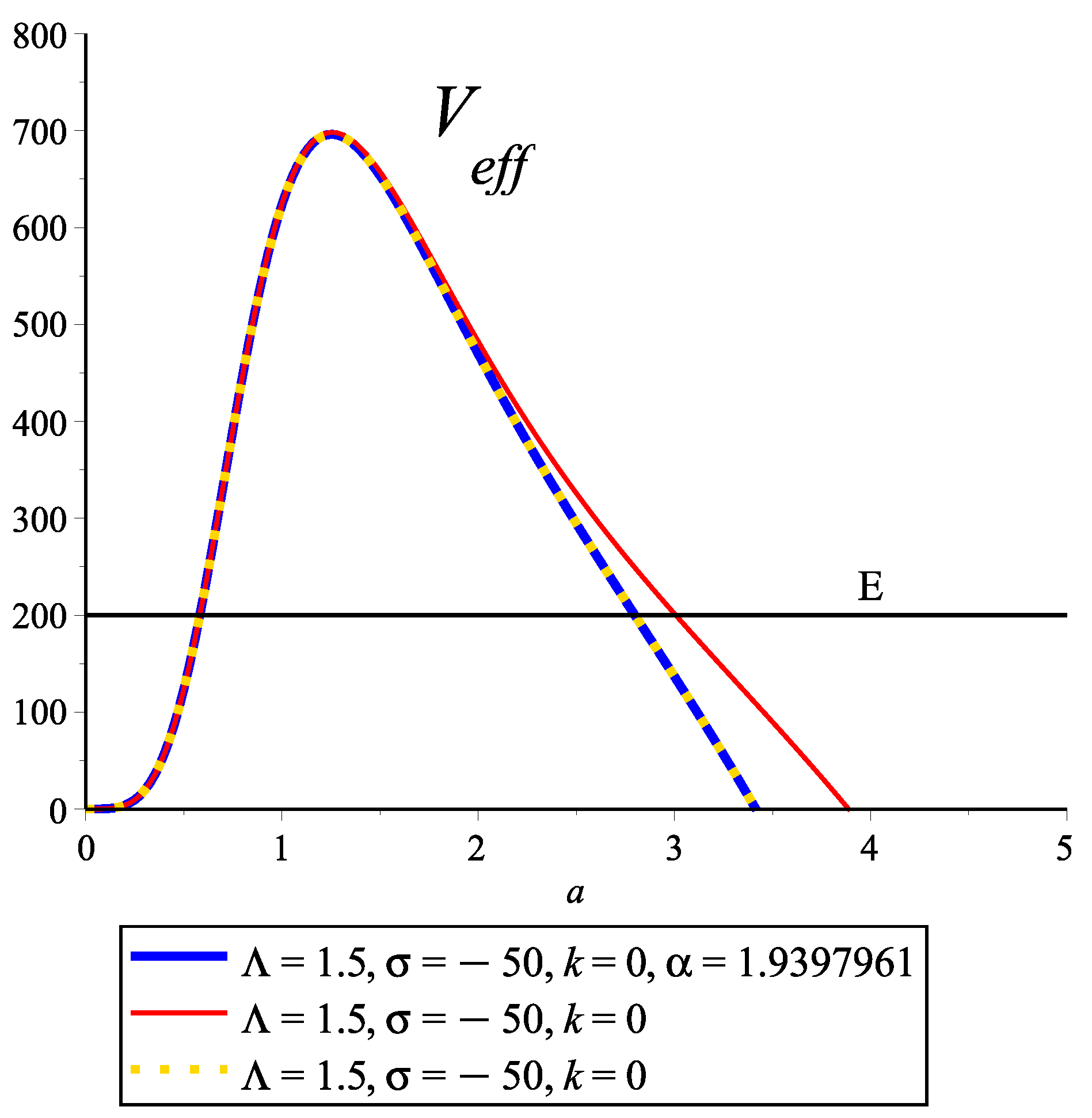
3.1. Tunneling Probability When
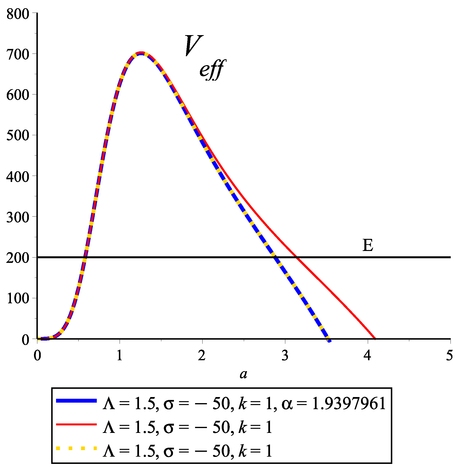
3.2. Tunneling Probability When
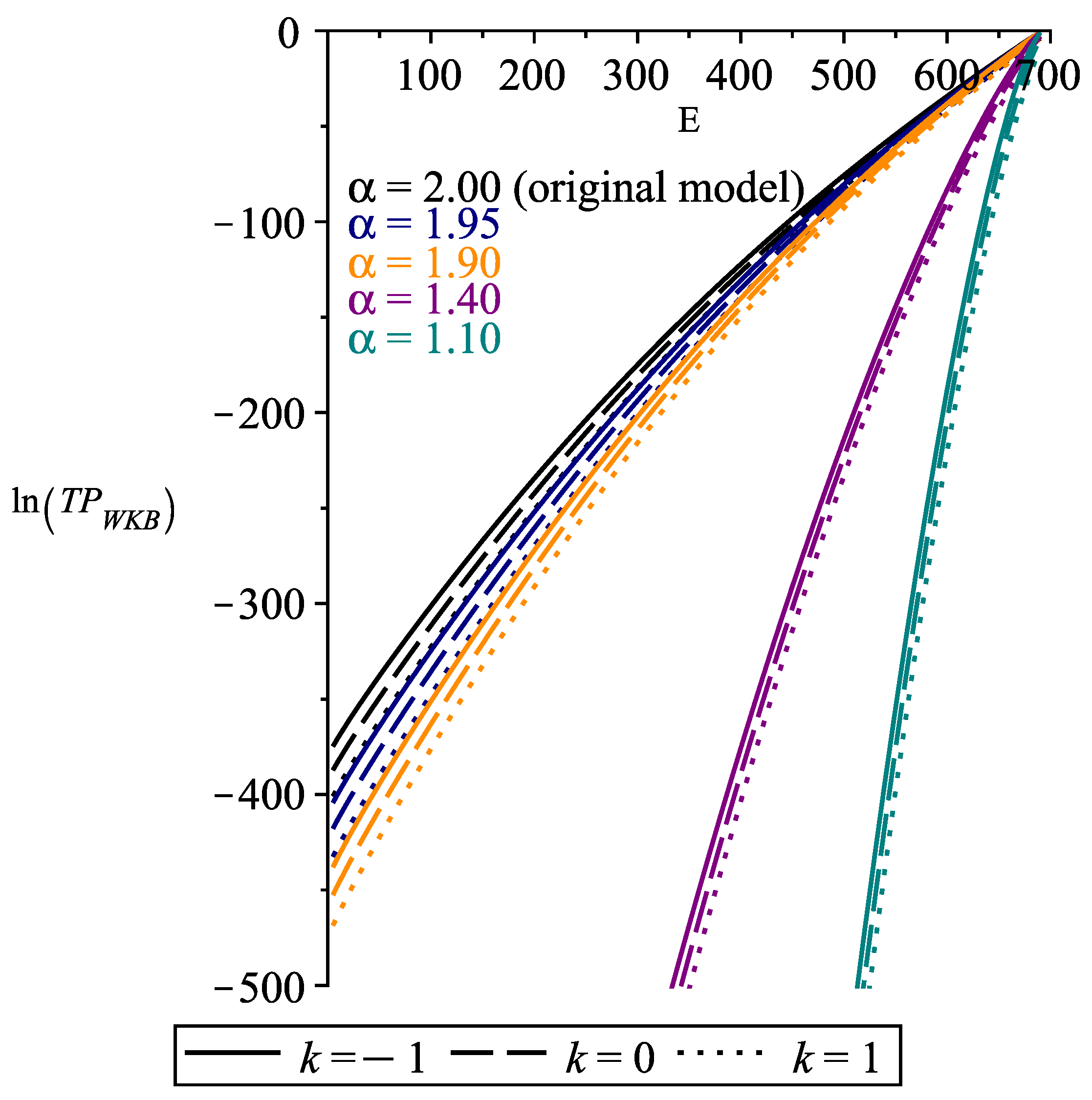
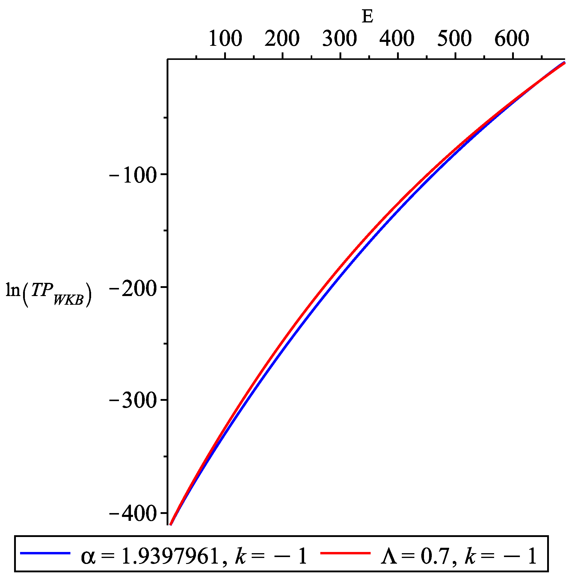
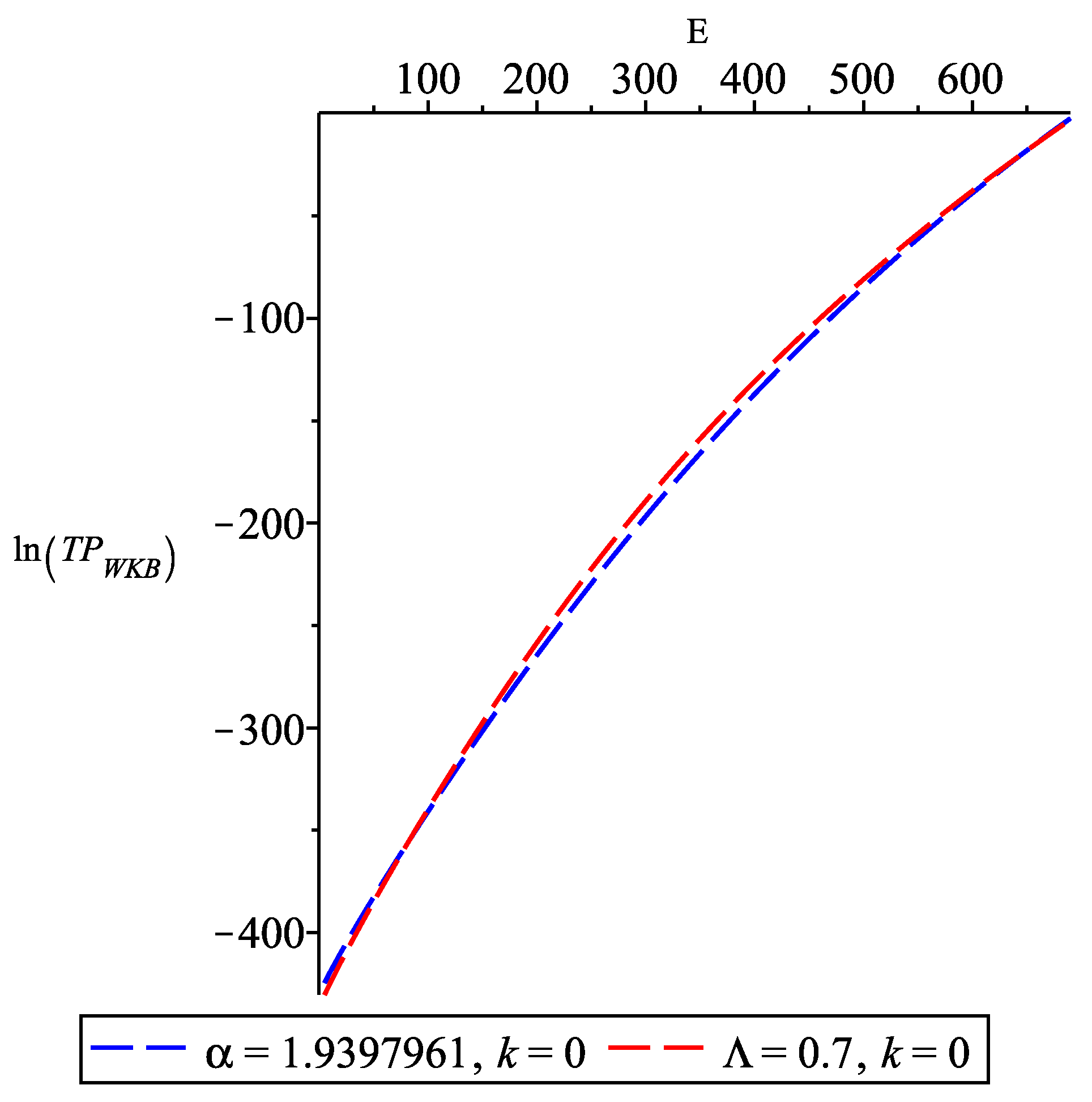
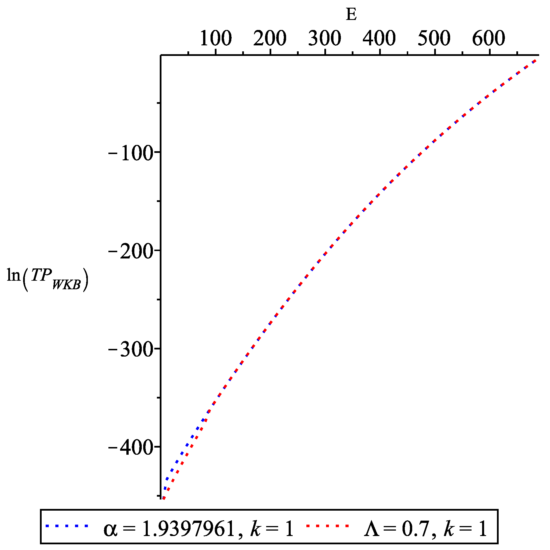
3.2.1. as a Function of E
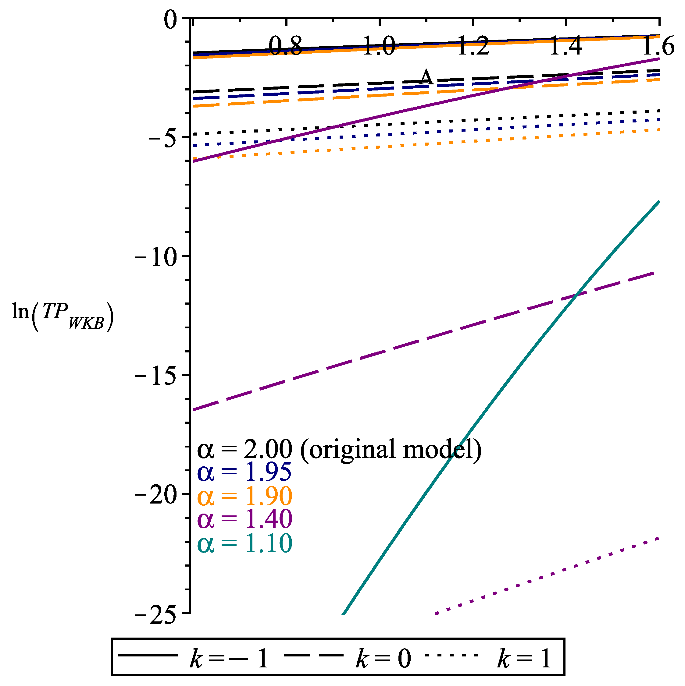
3.2.2. as a Function of
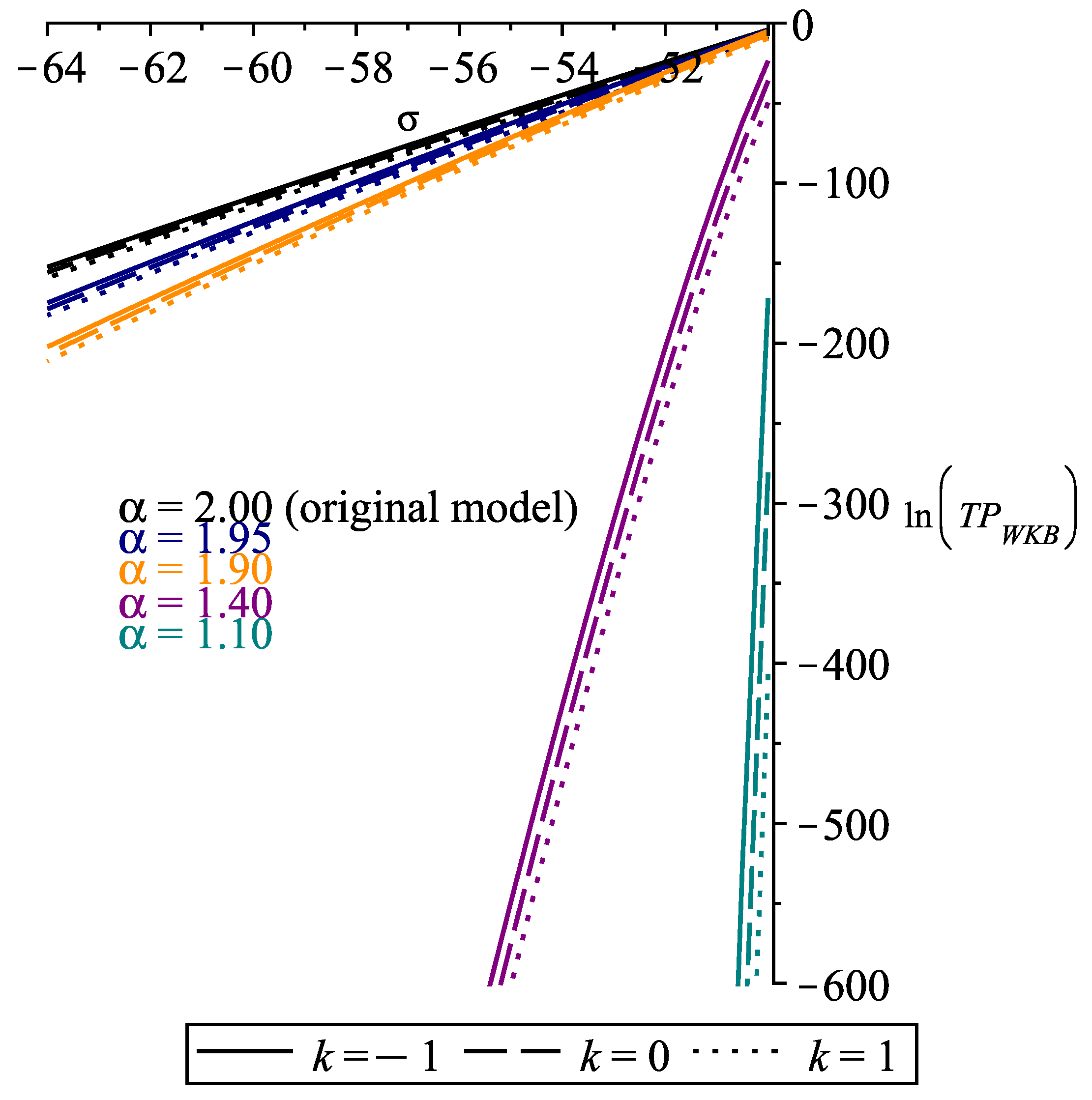
3.2.3. as a Function of
3.3. Analysis and Implication of the Riesz Derivative in the Calculation of the Tunneling Probability
- For hyperbolic space-like sections

| k | E | and | |
|---|---|---|---|
| −1 | 10 | ||
| 170 | |||
| 340 | |||
| 500 | |||
| 660 | 463.1719831 | 400.5848243 |
| k | E | and | |
|---|---|---|---|
| −1 | 10 | ||
| 170 | |||
| 340 | |||
| 500 | |||
| 660 | 0.000004661379104 | 0.000006231744824 |
- For flat space-like sections
| k | E | and | |
|---|---|---|---|
| 0 | 10 | ||
| 170 | |||
| 340 | |||
| 500 | |||
| 660 | 1191.527234 | 1069.113378 |
| k | E | and | |
|---|---|---|---|
| 0 | 10 | ||
| 170 | |||
| 340 | |||
| 500 | |||
| 660 |
- For spherical space-like sections
| k | E | and | |
|---|---|---|---|
| 1 | 10 | ||
| 170 | |||
| 340 | |||
| 500 | |||
| 660 | 3160.340886 | 2945.792223 |
| k | E | and | |
|---|---|---|---|
| 1 | 10 | ||
| 170 | |||
| 340 | |||
| 500 | |||
| 660 |
4. Conclusions and Discussions
Author Contributions
Funding
Data Availability Statement
Conflicts of Interest
Appendix A. Dα Analysis

References
- DeWitt, B.S. Quantum Theory of Gravity. I. The Canonical Theory. Phys. Rev. D 1967, 160, 1113. [Google Scholar] [CrossRef]
- Wheeler, J.A. Battelles Rencontres; DeWitt, C., Wheeler, J.A., Eds.; Benjamin: New York, NY, USA, 1968. [Google Scholar]
- Grishchuk, L.P.; Zeldovich, Y.B. Quantum Structure of Space and Time; Duff, M., Isham, C., Eds.; Cambridge University Press: Cambridge, UK, 1982. [Google Scholar]
- Hawking, S.W. Quantum Cosmology. In Relativity, Groups and Topology II: Proceedings of the 1983 Les Houches Summer School, Session XL; DeWitt, B.S., Stora, R., Eds.; North-Holland: Amsterdam, The Netherlands, 1984; pp. 333–379. [Google Scholar]
- Halliwell, J.; Hawking, S. Quantum Cosmology—Beyond Minisuperspace. In Proceedings of the Fourth Marcel Grossmann Meeting on General Relativity, Rome, Italy, 1985; Ruffini, R., Ed.; North-Holland: Amsterdam, The Netherlands, 1986; Part A, pp. 65–83. [Google Scholar]
- Bojowald, M. Quantum Cosmology: A Fundamental Description of the Universe; Lecture Notes in Physics; Springer: New York, NY, USA, 2011; Volume 835. [Google Scholar]
- Bojowald, M. Quantum cosmology: A review. Rep. Prog. Phys. 2015, 78, 023901. [Google Scholar] [CrossRef] [PubMed]
- Pinto-Neto, N.; Fabris, J.C. Quantum cosmology from the de Broglie–Bohm perspective. Class. Quantum Grav. 2013, 30, 143001. [Google Scholar] [CrossRef]
- Jalalzadeh, S.; Moniz, P.V. Challenging Routes in Quantum Cosmology; World Scientific Publishing Co. Pte. Ltd.: Singapore, 2023. [Google Scholar]
- Vilenkin, A. Creation of universes from nothing. Phys. Lett. B 1982, 117, 25. [Google Scholar] [CrossRef]
- Vilenkin, A. Quantum creation of universes. Phys. Rev. D 1984, 30, 509. [Google Scholar] [CrossRef]
- Vilenkin, A. Boundary conditions in quantum cosmology. Phys. Rev. D 1986, 33, 3560. [Google Scholar] [CrossRef]
- Linde, A.D. Quantum creation of the inflationary universe. Lett. Nuovo Cim. 1984, 39, 401. [Google Scholar] [CrossRef]
- Rubakov, V.A. Quantum mechanics in the tunneling universe. Phys. Lett. B 1984, 148, 280. [Google Scholar] [CrossRef]
- Monerat, G.A.; Alvarenga, F.G.; Gonçalves, S.V.B.; Oliveira-Neto, G.; Santos, C.G.M.; Silva, E.V.C. The effects of dark energy on the early Universe with radiation and an ad hoc potential. Eur. Phys. J. Plus 2022, 137, 117. [Google Scholar] [CrossRef]
- Chataignier, L.; Kiefer, C.; Moniz, P. Observations in quantum cosmology. Class. Quantum Grav. 2023, 40, 223001. [Google Scholar] [CrossRef]
- Herrman, R. Fractional Calculus: An Introduction for Physicists, 2nd ed.; World Scientific: Singapore, 2014. [Google Scholar]
- Rasouli, S.M.M.; Costa, E.W.d.; Moniz, P.; Jalalzadeh, S. Inflation and Fractional Quantum Cosmology. Fractal Fract. 2022, 6, 655. [Google Scholar] [CrossRef]
- González, E.; Leon, G.; Fernandez-Anaya, G. Exact Solutions and Cosmological Constraints in Fractional Cosmology. Fractal Fract. 2023, 7, 368. [Google Scholar] [CrossRef]
- Hilfer, R. Applications of Fractional Calculus in Physics; World Scientific: Singapore, 2000. [Google Scholar]
- Ross, B. A brief history and exposition of the fundamental theory of fractional calculus. In Fractional Calculus and Its Applications; Lecture Notes in Mathematics; Ross, B., Ed.; Springer: Berlin/Heidelberg, Germany, 1975; Volume 457. [Google Scholar]
- Ortigueira, D.M. Fractional Calculus for Scientists and Engineers; Springer: Dordrecht, The Netherlands; Berlin/Heidelberg, Germany; London, UK; New York, NY, USA, 2011. [Google Scholar]
- Laskin, N. Fractional Schrödinger equation. Phys. Rev. E 2002, 66, 056108. [Google Scholar] [CrossRef] [PubMed]
- Laskin, N. Principles of Fractional Quantum Mechanics. arXiv 2010, arXiv:1009.5533. [Google Scholar]
- Jalalzadeh, S.; Costa, E.W.O.; Moniz, P.V. de Sitter fractional quantum cosmology. Phys. Rev. D 2022, 105, L121901. [Google Scholar] [CrossRef]
- Rasouli, S.M.M.; Cheraghchi, S.; Moniz, P. Fractional Scalar Field Cosmology. Fractal Fract. 2024, 8, 281. [Google Scholar] [CrossRef]
- Jarad, F.; Abdeljawad, T.; Hammouch, Z. On a class of ordinary differential equations in the frame of Atangana–Baleanu fractional derivative. Chaos Solitons Fractals 2018, 117, 16–20. [Google Scholar] [CrossRef]
- Syam, M.I.; Al-Refai, M. Fractional differential equations with Atangana–Baleanu fractional derivative: Analysis and applications. Chaos Solitons Fractals X 2019, 2, 100013. [Google Scholar] [CrossRef]
- Kucche, K.D.; Sutar, S.T. Analysis of nolinear fractional differential equations involving Atangana-Baleanu-Caputo derivative. Chaos Solitons Fractals 2021, 143, 110556. [Google Scholar] [CrossRef]
- Gao, X.Y. Hetero-Bäcklund transformation, bilinear forms and multi-solitons for a (2+1)-dimensional generalized modified dispersive water-wave system for the shallow water. Chin. J. Phys. 2024, 92, 1233–1239. [Google Scholar] [CrossRef]
- Gao, X.Y. Open-Ocean Shallow-Water Dynamics via a (2+1)-Dimensional Generalized Variable-Coefficient Hirota-Satsuma-Ito System: Oceanic Auto-Bäcklund Transformation and Oceanic Solitons. China Ocean Eng. 2025; in press. [Google Scholar] [CrossRef]
- Gao, X.Y. In an Ocean or a River: Bilinear Auto-Bäcklund Transformations and Similarity Reductions on an Extended Time-Dependent (3+1)-Dimensional Shallow Water Wave Equation. China Ocean Eng. 2025, 39, 160–165. [Google Scholar] [CrossRef]
- Laskin, N. Fractional quantum mechanics. Phys. Rev. E 2000, 62, 3135–3145. [Google Scholar] [CrossRef] [PubMed]
- Laskin, N. Fractional quantum mechanics and Lévy path integrals. Phys. Lett. A 2000, 268, 298. [Google Scholar] [CrossRef]
- Rabei, E.M.; Altarazi, I.M.A.; Muslih, S.I.; Baleanu, D. Fractional WKB approximation. Nonlinear Dyn. 2009, 57, 171–175. [Google Scholar] [CrossRef]
- de Oliveira, E.C.; Vaz, J., Jr. Tunneling in fractional quantum mechanics. J. Phys. A Math. Theor. 2011, 44, 185303. [Google Scholar] [CrossRef]
- Hasan, M.; Mandal, B.P. Tunneling time in space fractional quantum mechanics. Phys. Lett. A 2018, 382, 248–252. [Google Scholar] [CrossRef]
- Duan, X.; Ma, C.; Huang, H.; Deng, K. Uniform Operator: Aligning Fractional Time Quantum Mechanics with Basic Physical Principles. SSRN 2024. preprint. [Google Scholar] [CrossRef]
- Costa, E.W.d.O.; Jalalzadeh, R.; Junior, P.F.d.; Rasouli, S.M.M.; Jalalzadeh, S. Estimated Age of the Universe in Fractional Cosmology. Fractal Fract. 2023, 7, 854. [Google Scholar] [CrossRef]
- Tare, J.D.; Esguerra, J.P.H. Transmission through locally periodic potentials in space-fractional quantum mechanics. Physical A 2014, 407, 43–53. [Google Scholar] [CrossRef]
- Piskunov, N. Differential and Integral Calculus; CBS Publishers and Distributors: New Delhi, India, 1996; Volume I, Chapter 3. [Google Scholar]
- Oliveira-Neto, G.; Canedo, D.L.; Monerat, G.A. Tunneling probabilities for the birth of universes with radiation, cosmological constant and an ad hoc potential. Eur. Phys. J. Plus 2023, 138, 400. [Google Scholar] [CrossRef]
- Misner, C.W.; Thorne, K.S.; Wheeler, J.A. Gravitation; W. H. Freeman: San Francisco, CA, USA, 1973. [Google Scholar]
- Schutz, B.F. Perfect Fluids in General Relativity: Velocity Potentials and a Variational Principle. Phys. Rev. D 1970, 2, 2762. [Google Scholar] [CrossRef]
- Schutz, B.F. Hamiltonian Theory of a Relativistic Perfect Fluid. Phys. Rev. D 1971, 4, 3559. [Google Scholar] [CrossRef]
- Moniz, P.V.; Jalalzadeh, S. From Fractional Quantum Mechanics to Quantum Cosmology: An Overture. Mathematics 2020, 8, 313. [Google Scholar] [CrossRef]
- Calcagni, G. Multifractional theories: An unconventional review. J. High Energ. Phys. 2017, 2017, 138. [Google Scholar] [CrossRef]
- Calcagni, G. Complex dimensions and their observability. Phys. Rev. D 2017, 96, 046001. [Google Scholar] [CrossRef]
- Merzbacher, E. Quantum Mechanics, 3rd ed.; John Wiley and Sons, Inc.: New York, NY, USA, 1998; Chapter 7. [Google Scholar]

Disclaimer/Publisher’s Note: The statements, opinions and data contained in all publications are solely those of the individual author(s) and contributor(s) and not of MDPI and/or the editor(s). MDPI and/or the editor(s) disclaim responsibility for any injury to people or property resulting from any ideas, methods, instructions or products referred to in the content. |
© 2025 by the authors. Licensee MDPI, Basel, Switzerland. This article is an open access article distributed under the terms and conditions of the Creative Commons Attribution (CC BY) license (https://creativecommons.org/licenses/by/4.0/).
Share and Cite
Canedo, D.L.; Moniz, P.; Oliveira-Neto, G. Quantum Creation of a Friedmann-Robertson-Walker Universe: Riesz Fractional Derivative Applied. Fractal Fract. 2025, 9, 349. https://doi.org/10.3390/fractalfract9060349
Canedo DL, Moniz P, Oliveira-Neto G. Quantum Creation of a Friedmann-Robertson-Walker Universe: Riesz Fractional Derivative Applied. Fractal and Fractional. 2025; 9(6):349. https://doi.org/10.3390/fractalfract9060349
Chicago/Turabian StyleCanedo, Daniel L., Paulo Moniz, and Gil Oliveira-Neto. 2025. "Quantum Creation of a Friedmann-Robertson-Walker Universe: Riesz Fractional Derivative Applied" Fractal and Fractional 9, no. 6: 349. https://doi.org/10.3390/fractalfract9060349
APA StyleCanedo, D. L., Moniz, P., & Oliveira-Neto, G. (2025). Quantum Creation of a Friedmann-Robertson-Walker Universe: Riesz Fractional Derivative Applied. Fractal and Fractional, 9(6), 349. https://doi.org/10.3390/fractalfract9060349