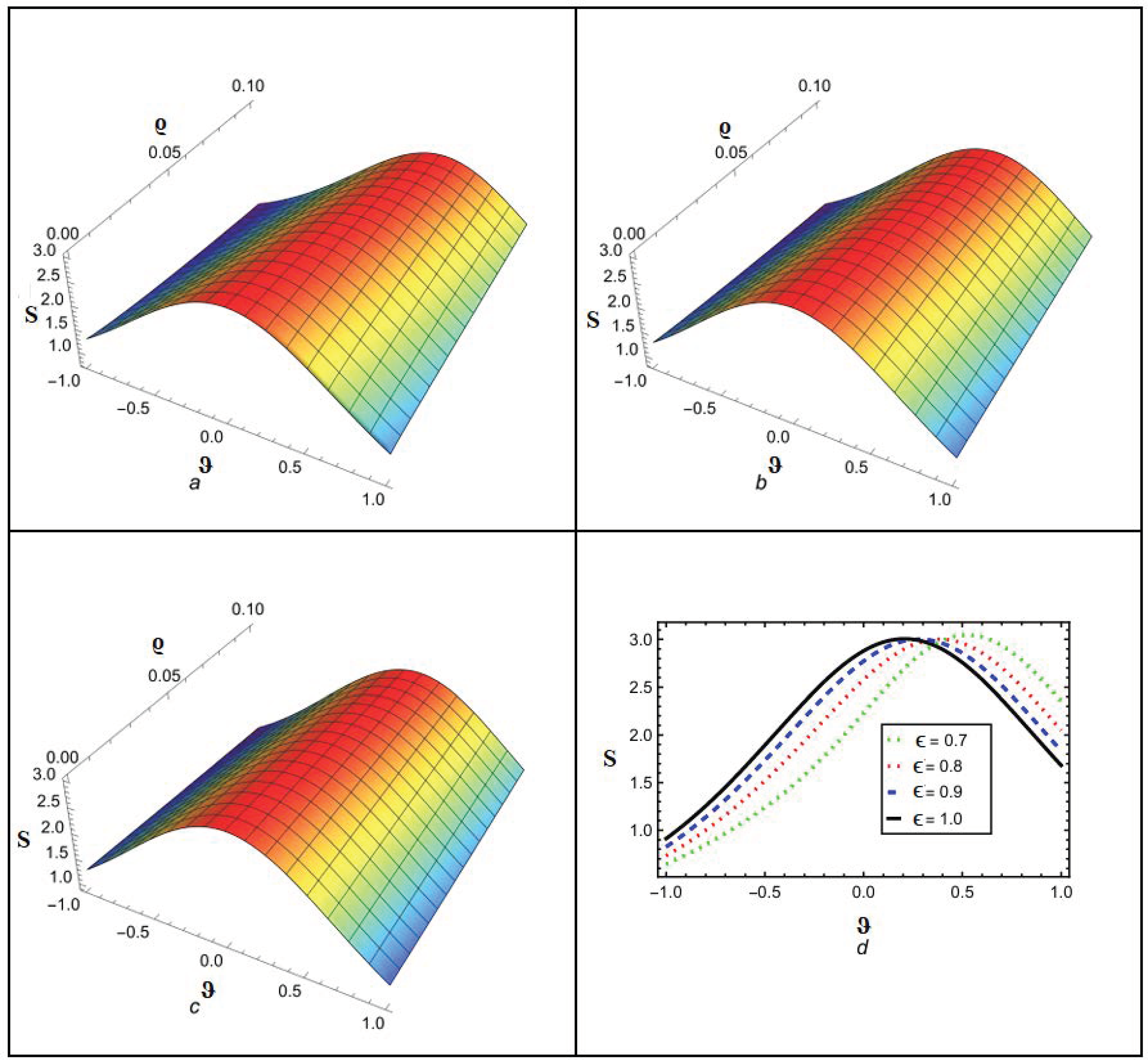
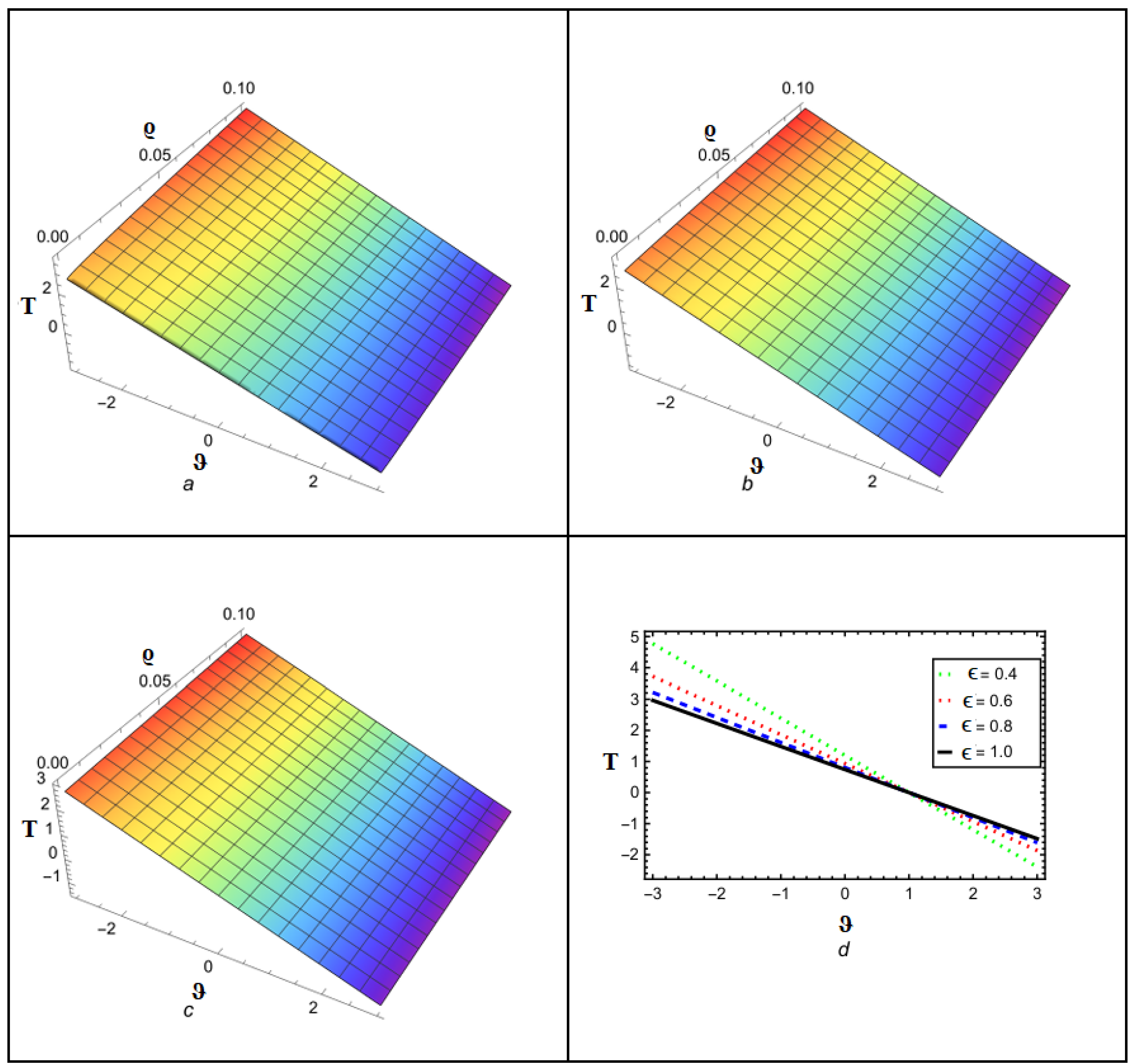
Figure 1.
Analytical solution behavior of NITM for at (a) ϵ = 0.8 (b) ϵ = 0.9 (c) ϵ = 1 (d) various values of ϵ.
Figure 1.
Analytical solution behavior of NITM for at (a) ϵ = 0.8 (b) ϵ = 0.9 (c) ϵ = 1 (d) various values of ϵ.
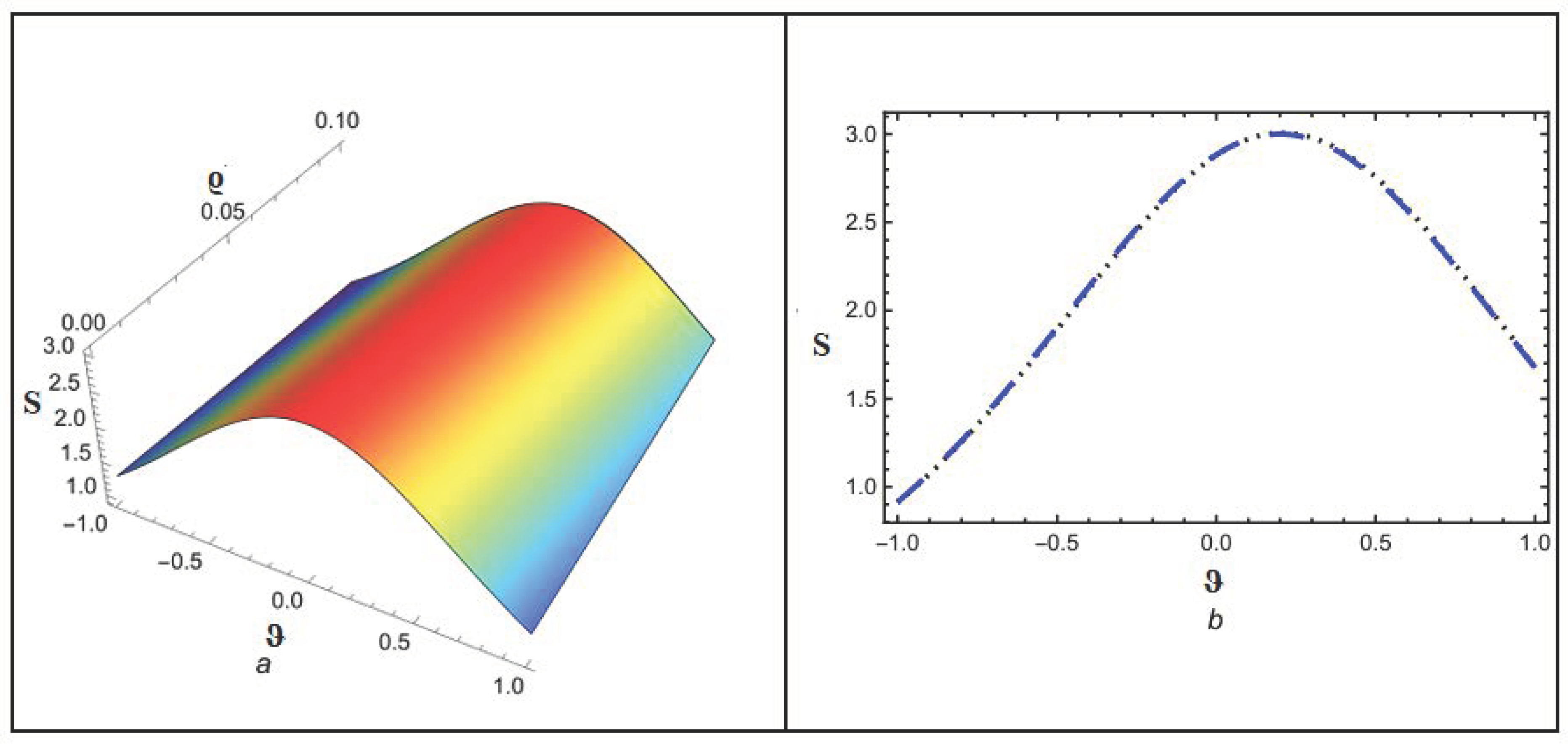
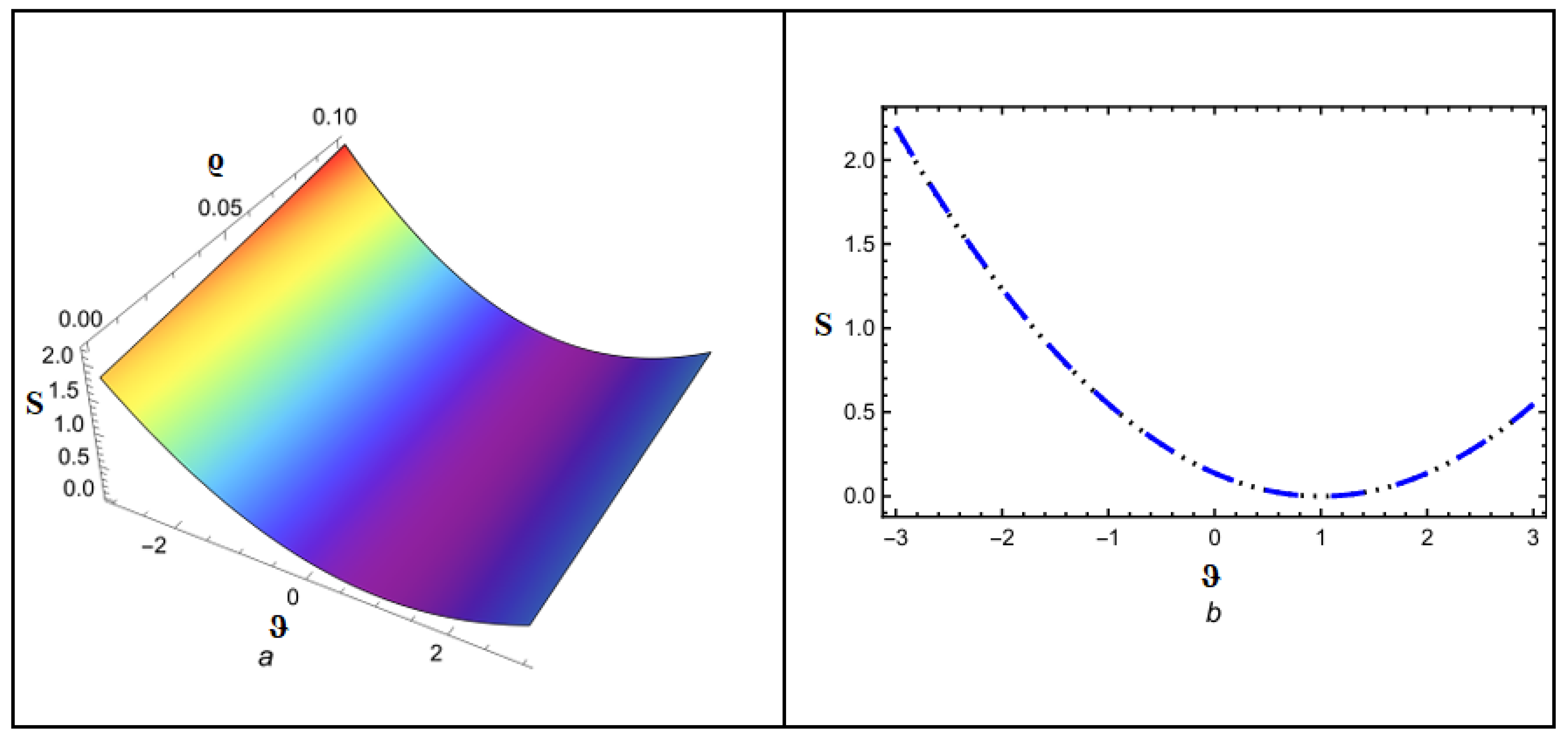
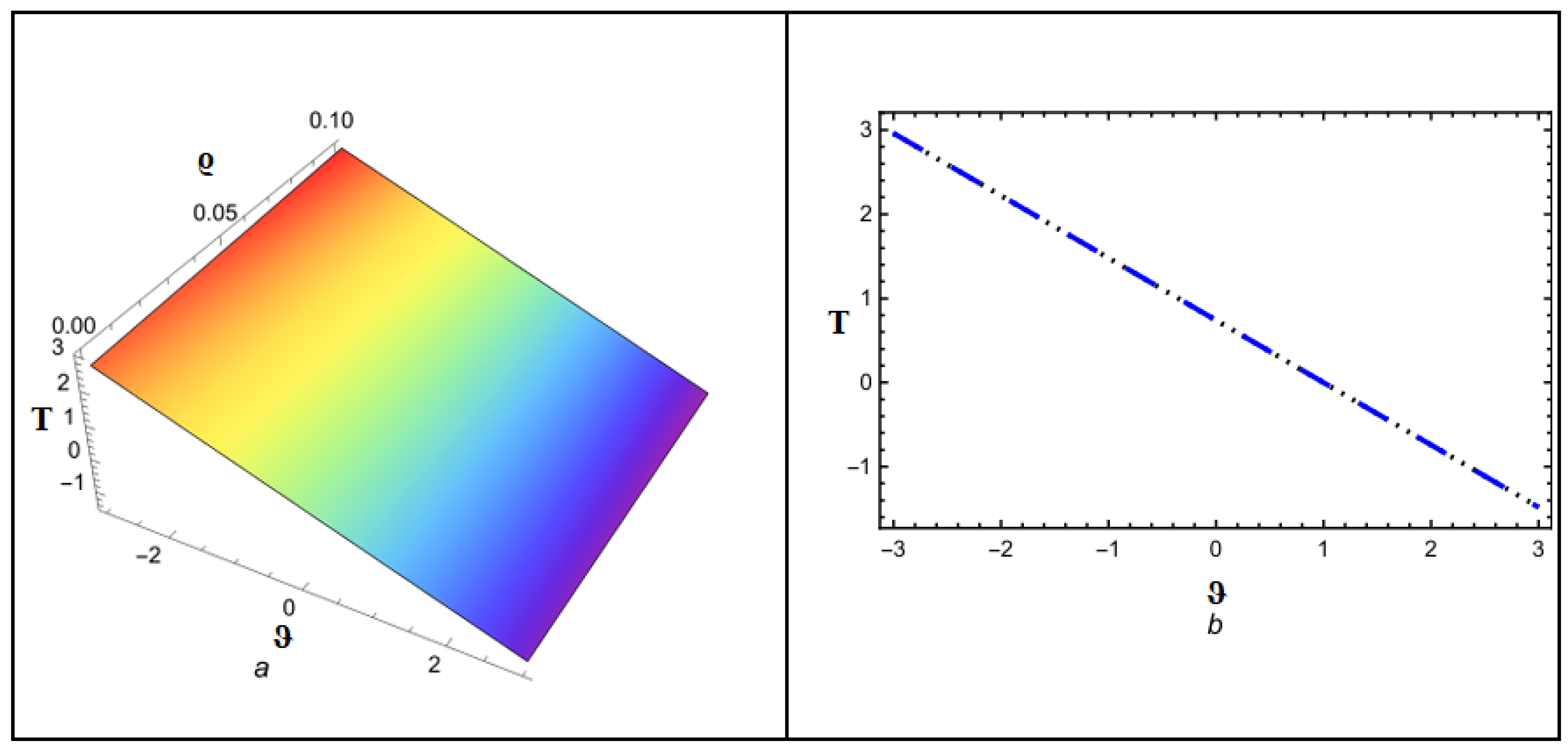
Figure 2.
(a,b) Accurate as well as analytical solution by NITM for .
Figure 2.
(a,b) Accurate as well as analytical solution by NITM for .
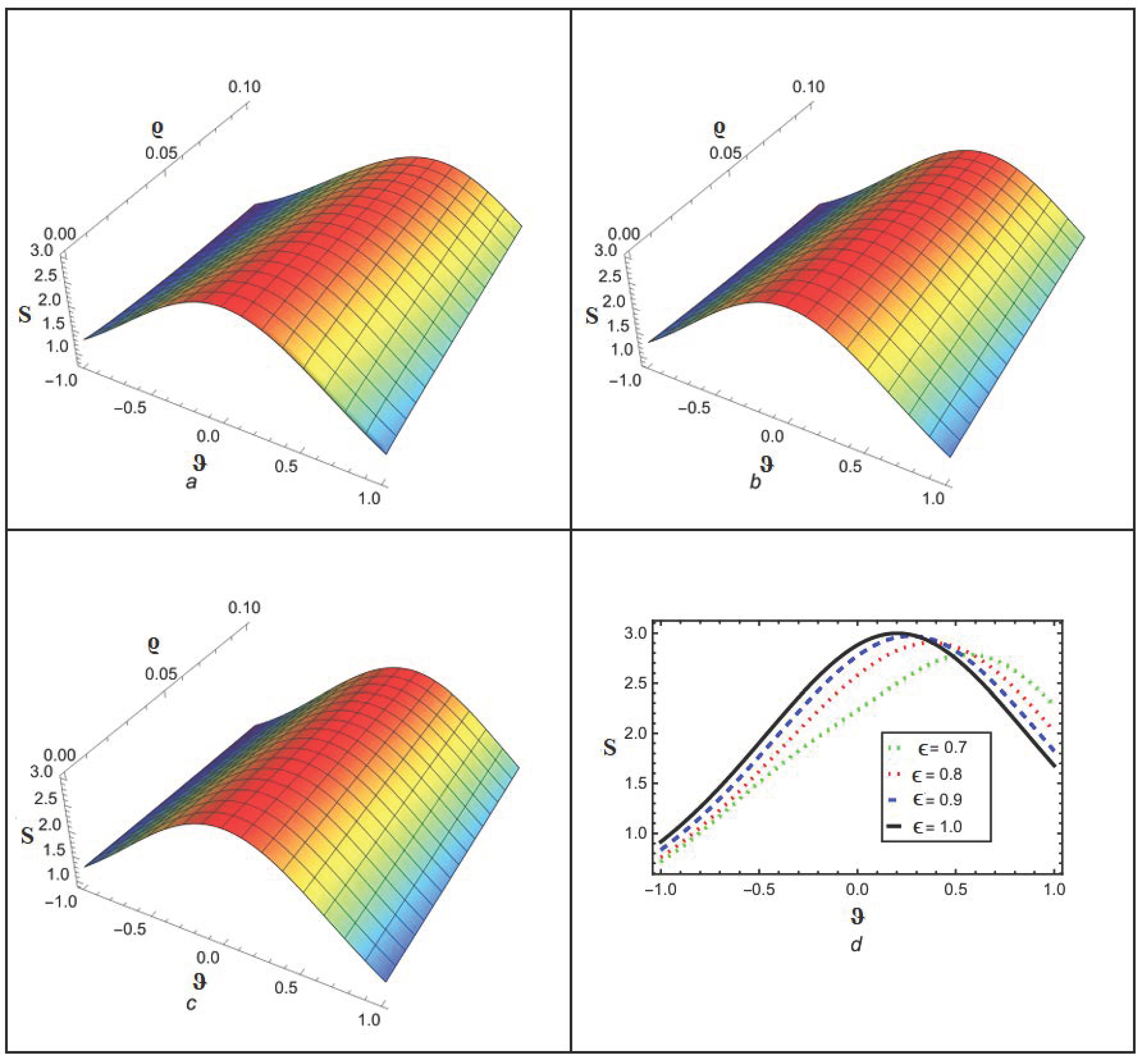
Figure 3.
Analytical solution behavior of ETDM for at (a) ϵ = 0.8 (b) ϵ = 0.9 (c) ϵ = 1 (d) various values of ϵ.
Figure 3.
Analytical solution behavior of ETDM for at (a) ϵ = 0.8 (b) ϵ = 0.9 (c) ϵ = 1 (d) various values of ϵ.
Figure 4.
(a,b) Accurate as well as analytical solution by ETDM for .
Figure 4.
(a,b) Accurate as well as analytical solution by ETDM for .
Figure 5.
Analytical solution behavior of NITM for at (a) ϵ = 0.8 (b) ϵ = 0.9 (c) ϵ = 1 (d) various values of ϵ.
Figure 5.
Analytical solution behavior of NITM for at (a) ϵ = 0.8 (b) ϵ = 0.9 (c) ϵ = 1 (d) various values of ϵ.
Figure 6.
(a,b) Accurate as well as analytical solution by NITM for .
Figure 6.
(a,b) Accurate as well as analytical solution by NITM for .
Figure 7.
Analytical solution behavior of ETDM for at (a) ϵ = 0.8 (b) ϵ = 0.9 (c) ϵ = 1 (d) various values of ϵ.
Figure 7.
Analytical solution behavior of ETDM for at (a) ϵ = 0.8 (b) ϵ = 0.9 (c) ϵ = 1 (d) various values of ϵ.
Figure 8.
(a,b) Accurate as well as analytical solution by ETDM for .
Figure 8.
(a,b) Accurate as well as analytical solution by ETDM for .
Figure 9.
Analytical solution behavior of NITM for at (a) ϵ = 0.8 (b) ϵ = 0.9 (c) ϵ = 1 (d) various values of ϵ.
Figure 9.
Analytical solution behavior of NITM for at (a) ϵ = 0.8 (b) ϵ = 0.9 (c) ϵ = 1 (d) various values of ϵ.
Figure 10.
(a,b) Accurate as well as analytical solution by NITM for .
Figure 10.
(a,b) Accurate as well as analytical solution by NITM for .
Figure 11.
Analytical solution behavior of ETDM for at (a) ϵ = 0.8 (b) ϵ = 0.9 (c) ϵ = 1 (d) various values of ϵ.
Figure 11.
Analytical solution behavior of ETDM for at (a) ϵ = 0.8 (b) ϵ = 0.9 (c) ϵ = 1 (d) various values of ϵ.
Figure 12.
(a,b) Accurate as well as analytical solution by ETDM for .
Figure 12.
(a,b) Accurate as well as analytical solution by ETDM for .
Figure 13.
Analytical solution behavior of NITM for at (a) ϵ = 0.8 (b) ϵ = 0.9 (c) ϵ = 1 (d) various values of ϵ.
Figure 13.
Analytical solution behavior of NITM for at (a) ϵ = 0.8 (b) ϵ = 0.9 (c) ϵ = 1 (d) various values of ϵ.
Figure 14.
(a,b) Accurate as well as analytical solution by NITM for .
Figure 14.
(a,b) Accurate as well as analytical solution by NITM for .
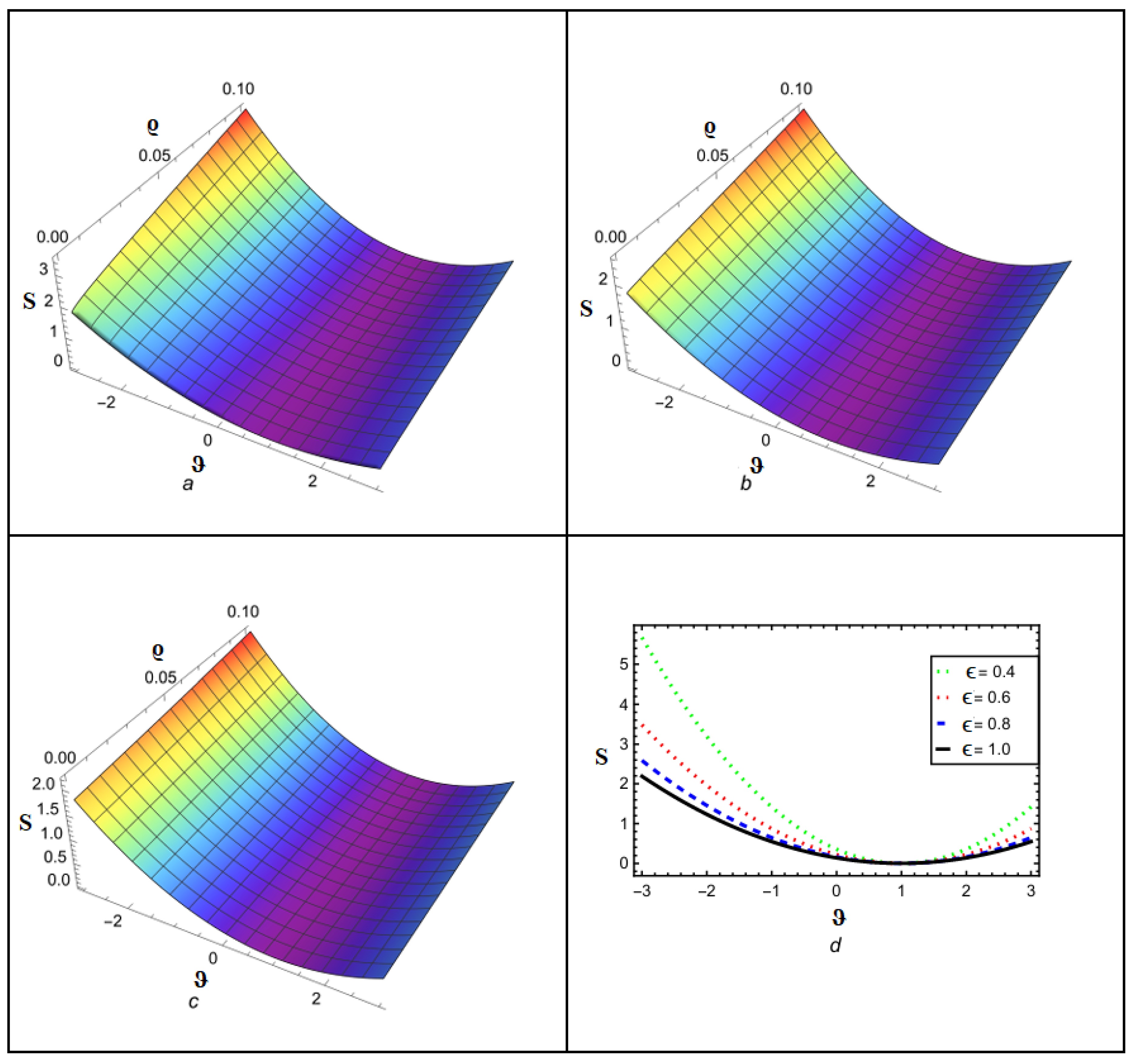
Figure 15.
Analytical solution behavior of ETDM for at (a) ϵ = 0.8 (b) ϵ = 0.9 (c) ϵ = 1 (d) various values of ϵ.
Figure 15.
Analytical solution behavior of ETDM for at (a) ϵ = 0.8 (b) ϵ = 0.9 (c) ϵ = 1 (d) various values of ϵ.
Figure 16.
(a,b) Accurate as well as analytical solution by ETDM for .
Figure 16.
(a,b) Accurate as well as analytical solution by ETDM for .
Table 1.
Accurate solution along with NITM solution at numerous orders of for .
Table 1.
Accurate solution along with NITM solution at numerous orders of for .
| | | | | |
|---|
| 0.0 | 3.0000000000 | 2.9964040800 | 2.9979184430 | 2.9988000000 | 2.9988003200 |
| 0.1 | 2.9701988730 | 2.9862500920 | 2.9834093360 | 2.9808860040 | 2.9808816240 |
| 0.2 | 2.8831289490 | 2.9175725200 | 2.9106003540 | 2.9048700200 | 2.9048616140 |
| 0.3 | 2.7454108850 | 2.7956573370 | 2.7850839530 | 2.7765796730 | 2.7765684510 |
| 0.4 | 2.5669163580 | 2.6294405240 | 2.6160196600 | 2.6053424550 | 2.6053298790 |
| 0.5 | 2.3593431990 | 2.4301774040 | 2.4147785420 | 2.4026124610 | 2.4025999210 |
| 0.6 | 2.1347332880 | 2.2099449710 | 2.1934453770 | 2.1804739570 | 2.1804625460 |
| 0.7 | 1.9042187700 | 1.9802880960 | 1.9634847600 | 1.9503240100 | 1.9503144140 |
| 0.8 | 1.6771655030 | 1.7512214490 | 1.7347736840 | 1.7219293630 | 1.7219218680 |
| 0.9 | 1.4607520830 | 1.5306671140 | 1.5150710680 | 1.5029206560 | 1.5029152310 |
| 1.0 | 1.2599230250 | 1.3242946060 | 1.3098840780 | 1.2986788210 | 1.2986752290 |
Table 2.
Accurate solution along with ETDM solution at numerous orders of for .
Table 2.
Accurate solution along with ETDM solution at numerous orders of for .
| | | | | |
|---|
| 0.0 | 2.9938145530 | 2.9964040800 | 2.9979184430 | 2.9988000000 | 2.9988003200 |
| 0.1 | 2.9891613720 | 2.9862233240 | 2.9833981130 | 2.9808813300 | 2.9808816240 |
| 0.2 | 2.9257584010 | 2.9175230820 | 2.9105796270 | 2.9048613880 | 2.9048616140 |
| 0.3 | 2.8084976120 | 2.7955923410 | 2.7850567040 | 2.7765683250 | 2.7765684510 |
| 0.4 | 2.6460176770 | 2.6293683540 | 2.6159894030 | 2.6053298540 | 2.6053298790 |
| 0.5 | 2.4494086370 | 2.4301059420 | 2.4147485810 | 2.4025999830 | 2.4025999210 |
| 0.6 | 2.2307189300 | 2.2098803150 | 2.1934182700 | 2.1804626680 | 2.1804625460 |
| 0.7 | 2.0015800170 | 1.9802339970 | 1.9634620790 | 1.9503145640 | 1.9503144140 |
| 0.8 | 1.7721713510 | 1.7511793950 | 1.7347560530 | 1.7219220200 | 1.7219218680 |
| 0.9 | 1.5506177240 | 1.5306368260 | 1.5150583700 | 1.5029153680 | 1.5029152310 |
| 1.0 | 1.3427948840 | 1.3242746780 | 1.3098757230 | 1.2986753420 | 1.2986752290 |
Table 3.
Accurate solution along with NITM solution at numerous orders of for .
Table 3.
Accurate solution along with NITM solution at numerous orders of for .
| | | | | |
|---|
| 0.0 | 1.9979381840 | 1.9988013600 | 1.9993061480 | 1.9996000670 | 1.9996000000 |
| 0.1 | 1.9963469540 | 1.9953856280 | 1.9944508290 | 1.9936170220 | 1.9936136620 |
| 0.2 | 1.9750281010 | 1.9722846220 | 1.9699540180 | 1.9680317120 | 1.9680260040 |
| 0.3 | 1.9350238390 | 1.9306221500 | 1.9270038120 | 1.9240819290 | 1.9240754130 |
| 0.4 | 1.8782093890 | 1.8723431300 | 1.8675981660 | 1.8638060980 | 1.8638003820 |
| 0.5 | 1.8070880220 | 1.8000018110 | 1.7943282680 | 1.7898230530 | 1.7898193530 |
| 0.6 | 1.7245421570 | 1.7165090690 | 1.7101237150 | 1.7050757740 | 1.7050746750 |
| 0.7 | 1.6335821890 | 1.6248810730 | 1.6180019120 | 1.6125815390 | 1.6125829990 |
| 0.8 | 1.5371273600 | 1.5280232740 | 1.5208550690 | 1.5152213780 | 1.5152249070 |
| 0.9 | 1.4378399520 | 1.4285698240 | 1.4212939010 | 1.4155871490 | 1.4155920420 |
| 1.0 | 1.3380200640 | 1.3287842350 | 1.3215527850 | 1.3158901820 | 1.3158957260 |
Table 4.
Accurate solution along with ETDM solution at numerous orders of for .
Table 4.
Accurate solution along with ETDM solution at numerous orders of for .
| | | | | |
|---|
| 0.0 | 1.9979381840 | 1.9988013600 | 1.9993061480 | 1.9996000000 | 1.9996000000 |
| 0.1 | 1.9963916830 | 1.9954045120 | 1.9944587460 | 1.9936169590 | 1.9936136620 |
| 0.2 | 1.9751048170 | 1.9723170110 | 1.9699675970 | 1.9680316590 | 1.9680260040 |
| 0.3 | 1.9351117460 | 1.9306592630 | 1.9270193720 | 1.9240818930 | 1.9240754130 |
| 0.4 | 1.8782866870 | 1.8723757640 | 1.8676118480 | 1.8638060800 | 1.8638003820 |
| 0.5 | 1.8071381840 | 1.8000229890 | 1.7943371470 | 1.7898230510 | 1.7898193530 |
| 0.6 | 1.7245572190 | 1.7165154280 | 1.7101263810 | 1.7050757850 | 1.7050746750 |
| 0.7 | 1.6335626690 | 1.6248728320 | 1.6179984570 | 1.6125815600 | 1.6125829990 |
| 0.8 | 1.5370798560 | 1.5280032180 | 1.5208466610 | 1.5152214050 | 1.5152249070 |
| 0.9 | 1.4377739580 | 1.4285419620 | 1.4212822200 | 1.4155871770 | 1.4155920420 |
| 1.0 | 1.3379452300 | 1.3287526410 | 1.3215395390 | 1.3158902100 | 1.3158957260 |
Table 5.
Comparative analysis of our methods solution with analytic and homotopy perturbation transform method (HPTM) solution for .
Table 5.
Comparative analysis of our methods solution with analytic and homotopy perturbation transform method (HPTM) solution for .
| | | | | |
|---|
| | −4 | 0.00286522 | 0.00386526 | 0.00386525 | 0.00386523 |
| | −3 | 0.0284431 | 0.0284434 | 0.0284433 | 0.0284432 |
| 0.01 | −2 | 0.203929 | 0.203931 | 0.203930 | 0.203930 |
| | −1 | 1.22192 | 1.22191 | 1.22191 | 1.22191 |
| | 0 | 2.9988 | 2.9988 | 2.9988 | 2.9988 |
| | −4 | 0.00371375 | 0.00371409 | 0.00371408 | 0.00371391 |
| | −3 | 0.0273329 | 0.0273353 | 0.0273352 | 0.0273340 |
| 0.02 | −2 | 0.196199 | 0.196213 | 0.196212 | 0.196205 |
| | −1 | 1.18467 | 1.18465 | 1.18465 | 1.18464 |
| | 0 | 2.99521 | 2.9952 | 2.9952 | 2.9952 |
Table 6.
Comparative analysis of our methods solution with analytic and homotopy perturbation transform method (HPTM) solution for .
Table 6.
Comparative analysis of our methods solution with analytic and homotopy perturbation transform method (HPTM) solution for .
| | | | | |
|---|
| | −4 | 0.0717887 | 0.0717888 | 0.0717888 | 0.00386523 |
| | −3 | 0.194741 | 0.194741 | 0.194741 | 0.194741 |
| 0.01 | −2 | 0.521446 | 0.521446 | 0.521446 | 0.521446 |
| | −1 | 1.27641 | 1.27641 | 1.27641 | 1.27641 |
| | 0 | 1.9996 | 1.9996 | 1.9996 | 1.9996 |
| | −4 | 0.0703681 | 0.0703689 | 0.0703688 | 0.0703688 |
| | −3 | 0.190903 | 0.190905 | 0.190904 | 0.190904 |
| 0.02 | −2 | 0.511467 | 0.511467 | 0.511470 | 0.511462 |
| | −1 | 1.25681 | 1.25681 | 1.25679 | 1.25676 |
| | 0 | 1.9984 | 1.9984 | 1.9984 | 1.9984 |
Table 7.
Accurate solution along with NITM solution at numerous orders of for .
Table 7.
Accurate solution along with NITM solution at numerous orders of for .
| | | | | |
|---|
| 0.0 | 0.1159736073 | 0.1148737650 | 0.1140243245 | 0.1133668148 | 0.1133671168 |
| 0.1 | 0.0939386218 | 0.0930477496 | 0.0923597028 | 0.0918271199 | 0.0918273646 |
| 0.2 | 0.0742231086 | 0.0735192096 | 0.0729755676 | 0.0725547614 | 0.0725549547 |
| 0.3 | 0.0568270675 | 0.0562881448 | 0.0558719189 | 0.0555497392 | 0.0555498872 |
| 0.4 | 0.0417504986 | 0.0413545554 | 0.0410487568 | 0.0408120533 | 0.0408121620 |
| 0.5 | 0.0289934018 | 0.0287184412 | 0.0285060811 | 0.0283417037 | 0.0283417792 |
| 0.6 | 0.0185557771 | 0.0183798024 | 0.0182438919 | 0.0181386903 | 0.0181387386 |
| 0.7 | 0.0104376245 | 0.0103386387 | 0.0102621891 | 0.0102030132 | 0.0102030405 |
| 0.8 | 0.0046389442 | 0.0045949505 | 0.0045609729 | 0.0045346725 | 0.0045346846 |
| 0.9 | 0.0011597360 | 0.0011487376 | 0.0011402432 | 0.0011336681 | 0.0011336711 |
| 1.0 | 0.0000000000 | 0.0000000000 | 0.0000000000 | 0.0000000000 | 0.0000000000 |
Table 8.
Accurate solution along with ETDM solution at numerous orders of for .
Table 8.
Accurate solution along with ETDM solution at numerous orders of for .
| | | | | |
|---|
| 0.0 | 0.1159718714 | 0.1148729961 | 0.1140239860 | 0.1133666667 | 0.1133671168 |
| 0.1 | 0.0939372158 | 0.0930471268 | 0.0923594286 | 0.0918269999 | 0.0918273646 |
| 0.2 | 0.0742219976 | 0.0735187175 | 0.0729753510 | 0.0725546666 | 0.0725549547 |
| 0.3 | 0.0568262169 | 0.0562877680 | 0.0558717531 | 0.0555496666 | 0.0555498872 |
| 0.4 | 0.0417498736 | 0.0413542785 | 0.0410486349 | 0.0408119999 | 0.0408121620 |
| 0.5 | 0.0289929678 | 0.0287182490 | 0.0285059965 | 0.0283416666 | 0.0283417792 |
| 0.6 | 0.0185554994 | 0.0183796794 | 0.0182438377 | 0.0181386666 | 0.0181387386 |
| 0.7 | 0.0104374683 | 0.0103385695 | 0.0102621586 | 0.0102029999 | 0.0102030405 |
| 0.8 | 0.0046388748 | 0.0045949198 | 0.0045609593 | 0.0045346666 | 0.0045346846 |
| 0.9 | 0.0011597187 | 0.0011487299 | 0.0011402398 | 0.0011336666 | 0.0011336711 |
| 1.0 | 0.0000000000 | 0.0000000000 | 0.0000000000 | 0.0000000000 | 0.0000000000 |
Table 9.
Accurate solution along with NITM solution at numerous orders of for .
Table 9.
Accurate solution along with NITM solution at numerous orders of for .
| | | | | |
|---|
| 0.0 | 0.6810788654 | 0.6778532040 | 0.6753478089 | 0.6734001482 | 0.6734006734 |
| 0.1 | 0.6129709789 | 0.6100678836 | 0.6078130280 | 0.6060601334 | 0.6060606061 |
| 0.2 | 0.5448630923 | 0.5422825632 | 0.5402782471 | 0.5387201186 | 0.5387205387 |
| 0.3 | 0.4767552058 | 0.4744972428 | 0.4727434662 | 0.4713801037 | 0.4713804714 |
| 0.4 | 0.4086473192 | 0.4067119224 | 0.4052086853 | 0.4040400889 | 0.4040404040 |
| 0.5 | 0.3405394327 | 0.3389266020 | 0.3376739045 | 0.3367000741 | 0.3367003367 |
| 0.6 | 0.2724315462 | 0.2711412816 | 0.2701391236 | 0.2693600593 | 0.2693602694 |
| 0.7 | 0.2043236596 | 0.2033559612 | 0.2026043427 | 0.2020200445 | 0.2020202020 |
| 0.8 | 0.1362157731 | 0.1355706408 | 0.1350695618 | 0.1346800296 | 0.1346801347 |
| 0.9 | 0.0681078865 | 0.0677853204 | 0.0675347809 | 0.0673400148 | 0.0673400673 |
| 1.0 | 0.0000000000 | 0.0000000000 | 0.0000000000 | 0.0000000000 | 0.0000000000 |
Table 10.
Accurate solution along with ETDM solution at numerous orders of for .
Table 10.
Accurate solution along with ETDM solution at numerous orders of for .
| | | | | |
|---|
| 0.0 | 0.6810771295 | 0.6778524351 | 0.6753474704 | 0.6734000001 | 0.6734006734 |
| 0.1 | 0.6129694166 | 0.6100671916 | 0.6078127234 | 0.6060600001 | 0.6060606061 |
| 0.2 | 0.5448617036 | 0.5422819481 | 0.5402779763 | 0.5387200001 | 0.5387205387 |
| 0.3 | 0.4767539907 | 0.4744967046 | 0.4727432293 | 0.4713800001 | 0.4713804714 |
| 0.4 | 0.4086462777 | 0.4067114611 | 0.4052084822 | 0.4040400001 | 0.4040404040 |
| 0.5 | 0.3405385647 | 0.3389262175 | 0.3376737352 | 0.3367000001 | 0.3367003367 |
| 0.6 | 0.2724308518 | 0.2711409740 | 0.2701389882 | 0.2693600000 | 0.2693602694 |
| 0.7 | 0.2043231389 | 0.2033557305 | 0.2026042411 | 0.2020200000 | 0.2020202020 |
| 0.8 | 0.1362154259 | 0.1355704870 | 0.1350694941 | 0.1346800000 | 0.1346801347 |
| 0.9 | 0.0681077129 | 0.0677852435 | 0.0675347470 | 0.0673400000 | 0.0673400673 |
| 1.0 | 0.0000000000 | 0.0000000000 | 0.0000000000 | 0.0000000000 | 0.0000000000 |


