
Multifractal Analysis of Geological Data Using a Moving Window Dynamical Approach

 , , , , , , , ,
  and
and
Abstract
1. Introduction
2. Methodology
2.1. Dynamical Approach Method
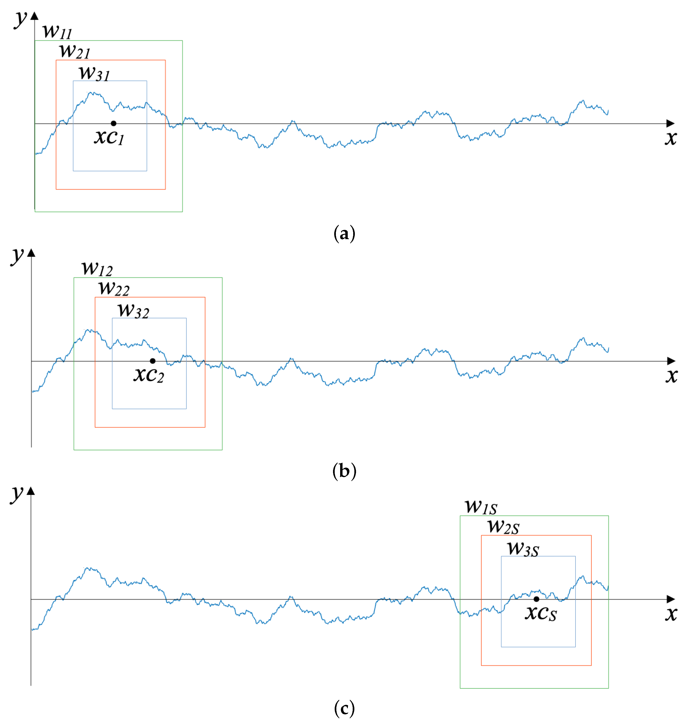
2.2. Moving Windows-Based Strategy
- First phase: Evaluate , which is the average fractal dimension associated with the data within the window , centered at . Thus, is related to (see Figure 1).
- Second phase: Define a new set of windows , centered at . This new set of windows is obtained by shifting all windows from the previous set by positions.
- Third phase: Evaluate , which is the average fractal dimension associated with the data within the window , centered at . Thus, is related to .
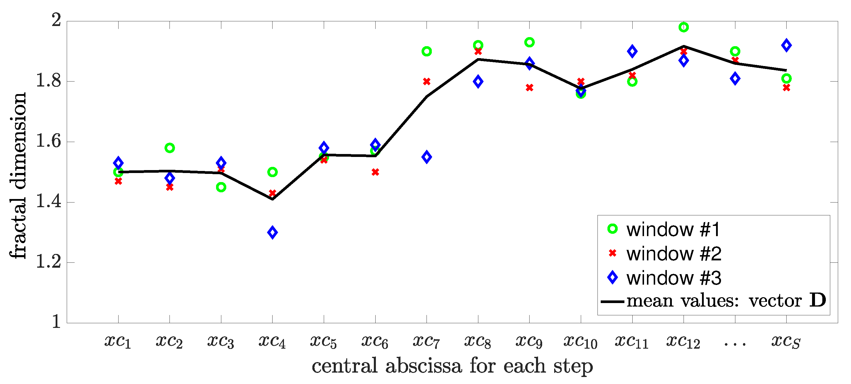
- Fourth phase: Repeat the second and third phases for subsequent steps, until the step is reached. Hence, a vector with fractal dimensions , respectively, associated with the vector is obtained.
- •
- The number of windows W. There must be a balance between computational efficiency and the accuracy of the vector . A larger W will comprise more data points, potentially improving the reliability of the fractal dimension estimates for . However, it will also increase the computational load. Thus, selecting W involves a trade-off: minimizing computational costs without compromising the accuracy of the estimates for .
- •
- The window size. The window size should be selected based on the desired resolution and the intrinsic characteristics of the data. Larger windows capture broader trends in fractal dimensions but may smooth out local details. Smaller windows are more sensitive to local variations but may be more susceptible to noise and imprecision inherent in the calculation of fractal dimension with few data points.
- •
- The step size . This parameter dictates the amount by which the windows are shifted along the dataset at each step. Typically, is less than or equal to the length of the smallest window to ensure overlapping, which provides smoother transitions between segments. The choice of is a trade-off between available computational resources and the desired resolution for locating points that indicate a change in the fractal behavior of the signal.
3. Validation
- •
- Number of windows. After several preliminary numerical tests, it was verified that six windows provided a good precision for the evaluation of fractal dimensions without significantly increasing the computational costs.
- •
- Window size. Two analyses were conducted to evaluate the methodology using windows with smaller lengths and larger lengths. For smaller windows, six windows were used with lengths of 401, 501, 601, 701, 801, and 901 data points. For larger windows, sizes of 1001, 1101, 1201, 1301, 1401, and 1501 data points were adopted.
- •
- The step size. To ensure a robust description of the multifractality, the number of steps was adjusted according to the domain size. By using , it resulted in 155 components for smaller windows and 149 for larger ones, providing sufficient detail for the vector .
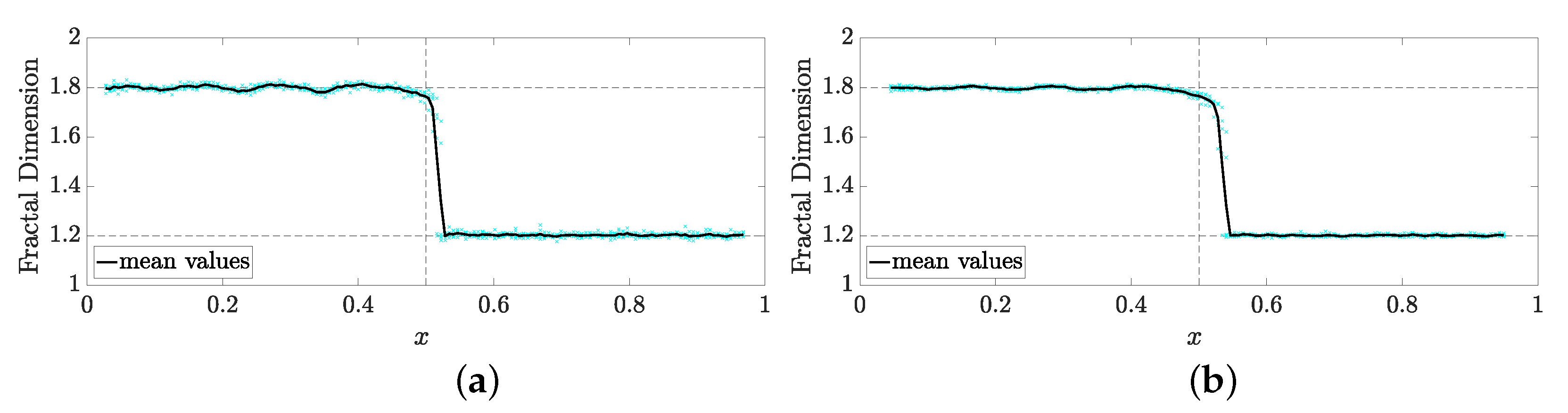
3.1. Case 1
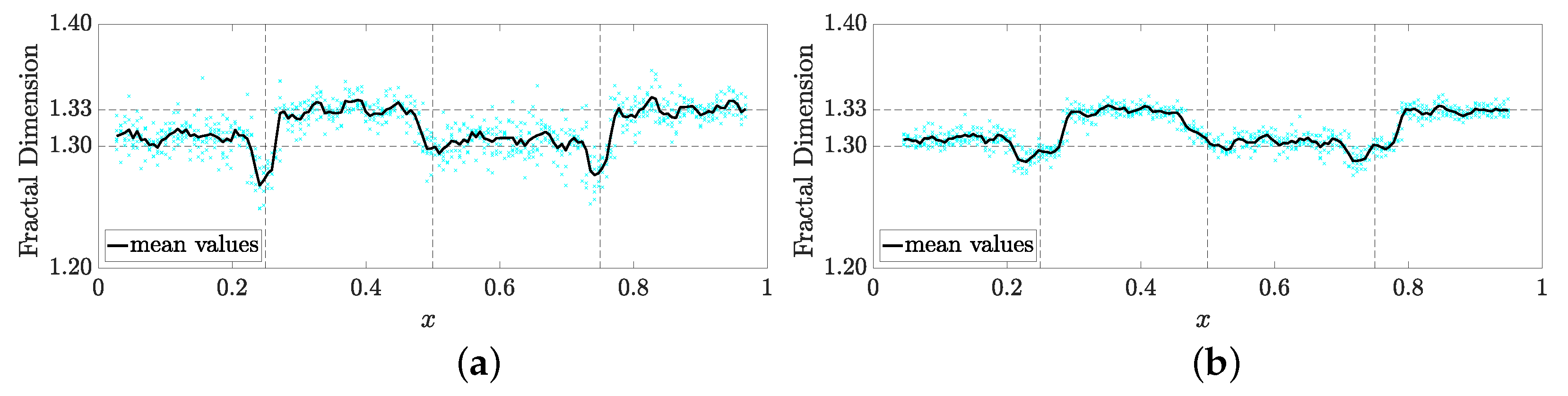
3.2. Case 2
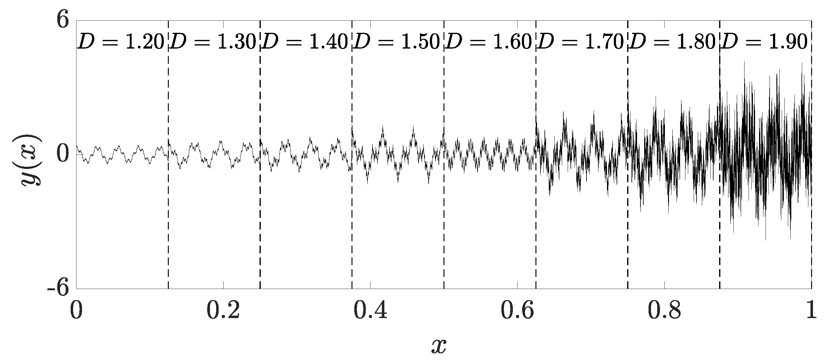
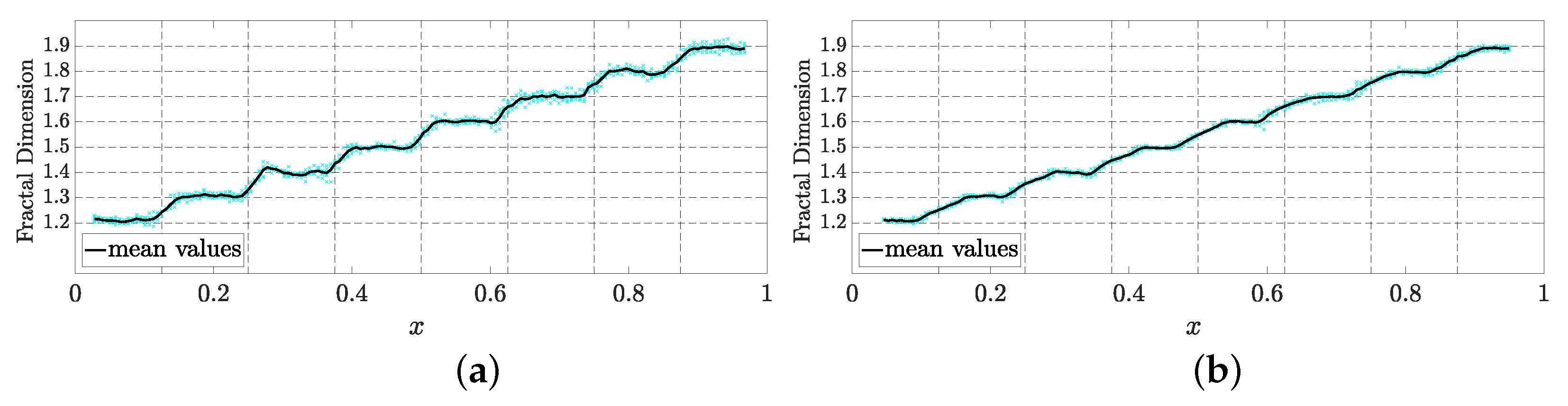
3.3. Case 3
3.4. Case 4
4. Multifractality of Geological Data
- Number of windows. This number was kept at 6 (six).
- Window size. Smaller windows were used (401, 501, 601, 701, 801, and 901 data points) to focus on local variations in fractal behavior.
- The step size. A step size of was used to provide sufficient detail for the fractal dimension vector .
4.1. Evaluation of Well #1
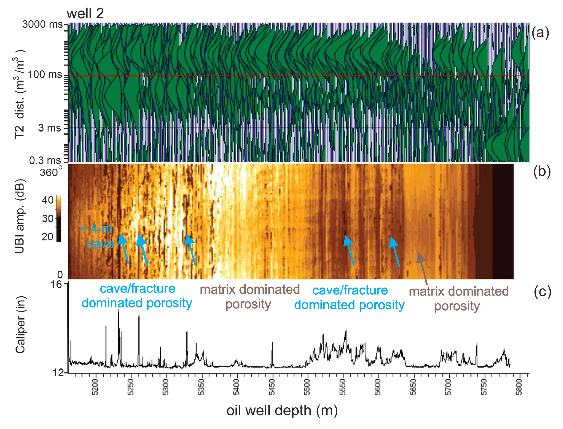
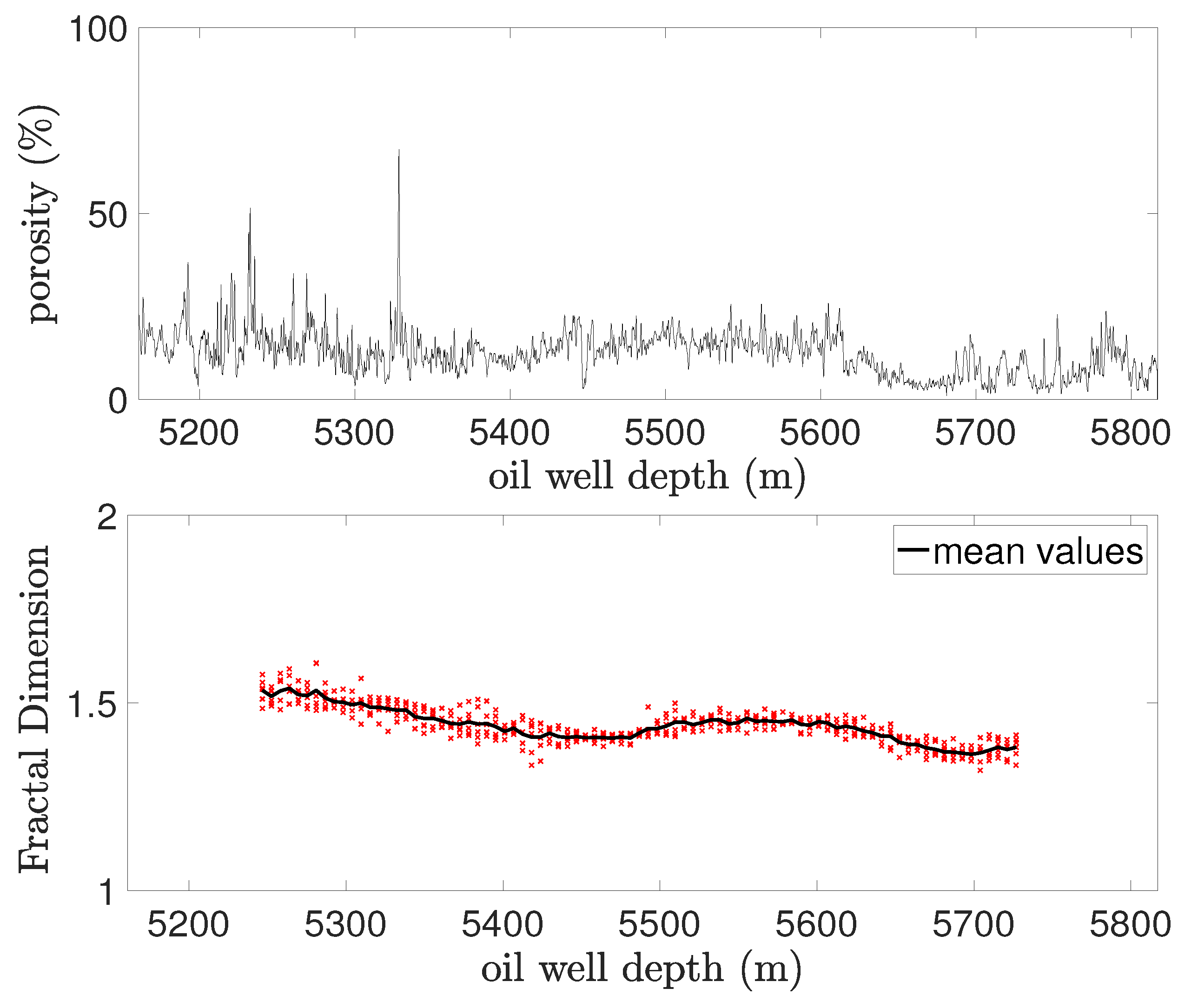
4.2. Evaluation of Well #2
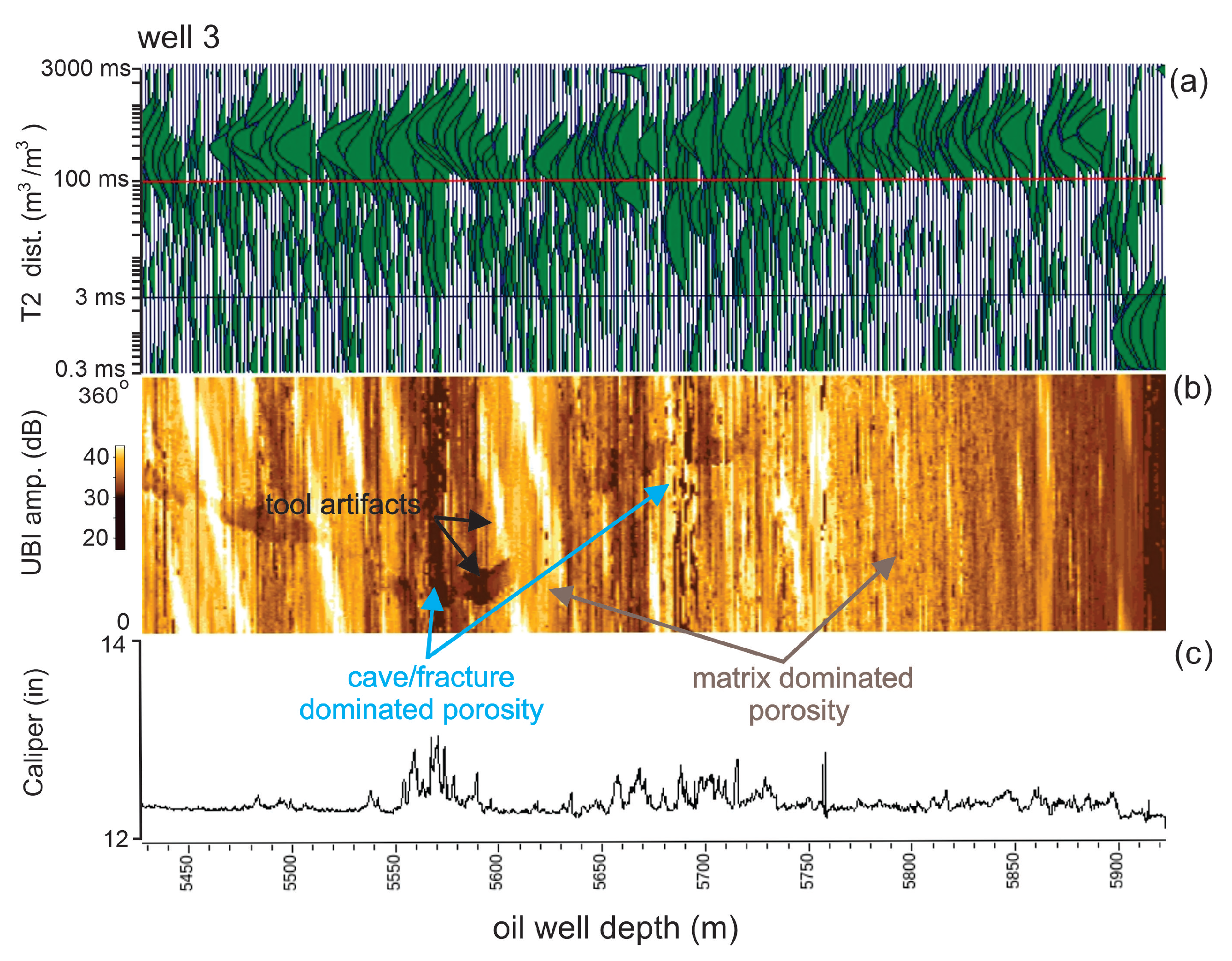
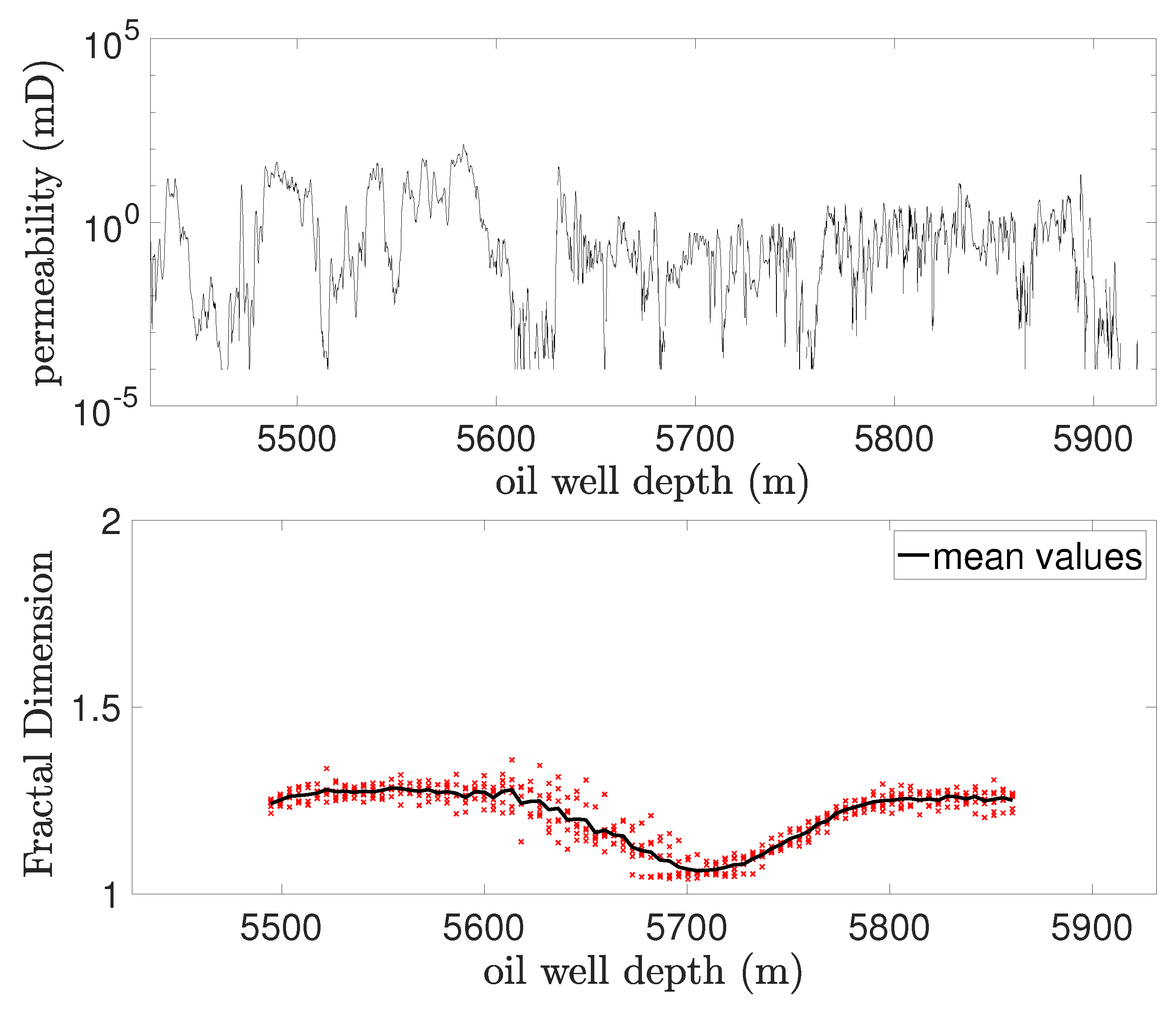
4.3. Evaluation of Well #3
5. Conclusions
Author Contributions
Funding
Data Availability Statement
Conflicts of Interest
References
- Ji, X.; Wang, H.; Ge, Y.; Liang, J.; Xu, X. Empirical mode decomposition-refined composite multiscale dispersion entropy analysis and its application to geophysical well log data. J. Pet. Sci. Eng. 2022, 208, 109495. [Google Scholar] [CrossRef]
- Dai, W.; Shen, Y.; Win, M. A Computational Geometry Framework for Efficient Network Localization. IEEE Trans. Inf. Theory 2018, 64, 1317–1339. [Google Scholar] [CrossRef]
- Ma, J.; Jiang, X.; Gong, M. Two-phase clustering algorithm with density exploring distance measure. CAAI Trans. Intell. Technol. 2018, 3, 59–64. [Google Scholar] [CrossRef]
- Subhakar, D.; Chandrasekhar, E. Reservoir characterization using multifractal detrended fluctuation analysis of geophysical well-log data. Phys. A Stat. Mech. Its Appl. 2016, 445, 57–65. [Google Scholar] [CrossRef]
- Habib, M.; Guangqing, Y.; Xie, C.; Charles, S.; Jakada, H.; Danlami, M.; Ahmed, H.; Omeiza, I. Optimizing oil and gas field management through a fractal reservoir study model. J. Pet. Explor. Prod. Technol. 2016, 7, 43–53. [Google Scholar] [CrossRef]
- Dimri, V. Fractal Solutions for Understanding Complex Systems in Earth Sciences; Springer: Berlin/Heidelberg, Germany, 2016. [Google Scholar]
- Wu, B.; Xie, R.; Wang, X.; Wang, T.; Yue, W. Characterization of pore structure of tight sandstone reservoirs based on fractal analysis of NMR echo data. J. Nat. Gas Sci. Eng. 2020, 81, 103483. [Google Scholar] [CrossRef]
- Boulassel, A.; Zaourar, N.; Gaci, S.; Boudella, A. A new multifractal analysis-based for identifying the reservoir fluid nature. J. Appl. Geophys. 2021, 185, 104185. [Google Scholar] [CrossRef]
- Marsan, D.; Bean, C. Multiscaling nature of sonic velocities and lithology in the upper crystalline crust: Evidence from the KTB main borehole. Geophys. Res. Lett. 1999, 26, 275–278. [Google Scholar] [CrossRef]
- Guadagnini, A.; Neuman, S.; Riva, M. Numerical investigation of apparent multifractality of samples from processes subordinated to truncated fBm. Hydrol. Processes 2011, 26, 2894–2908. [Google Scholar] [CrossRef]
- Elyas, H.; Hossein, H.; Yousef, S.; Seyed, J. Self-similar segmentation and multifractality of post-stack seismic data. Pet. Explor. Dev. 2020, 47, 781–790. [Google Scholar] [CrossRef]
- Boufadel, M.; Lu, S.; Molz, F.; Lavallee, D. Multifractal scaling of the intrinsic permeability. Water Resour. Res. 2000, 36, 3211–3222. [Google Scholar] [CrossRef]
- Dashtian, H.; Jafari, G.; Sahimi, M.; Masihi, M. Scaling, multifractality, and long-range correlations in well log data of large-scale porous media. Phys. A Stat. Mech. Its Appl. 2011, 390, 2096–2111. [Google Scholar] [CrossRef]
- Zaourar, N.; Hamoudi, M.; Briqueu, L. Détection des transitions lithologiques par l’analyse de la composante fractale des diagraphies par transformée continue en ondelettes. Comptes Rendus Géosci. 2006, 338, 514–520. [Google Scholar] [CrossRef]
- Sha, F.; Xiao, L.; Mao, Z.; Jia, C. Petrophysical Characterization and Fractal Analysis of Carbonate Reservoirs of the Eastern Margin of the Pre-Caspian Basin. Energies 2018, 12, 78. [Google Scholar] [CrossRef]
- Mahsal Khan, M.; Fadzil, A.; Hani, M.; Firdaus, M.; Halim, M. Using Singularity Spectrum Attributes for Analyzing Homogeneity/Heterogeneity of Reservoir. ASEG Ext. Abstr. 2007, 2007, 1–4. [Google Scholar] [CrossRef]
- Ojha, S.; Misra, S.; Tinni, A.; Sondergeld, C.; Rai, C. Pore connectivity and pore size distribution estimates for Wolfcamp and Eagle Ford shale samples from oil, gas and condensate windows using adsorption-desorption measurements. J. Pet. Sci. Eng. 2017, 158, 454–468. [Google Scholar] [CrossRef]
- Golsanami, N.; Fernando, S.; Jayasuriya, M.; Yan, W.; Dong, H.; Cui, L.; Dong, X.; Barzgar, E. Fractal Properties of Various Clay Minerals Obtained from SEM Images. Geofluids 2021, 2021, 5516444. [Google Scholar] [CrossRef]
- Xie, W.; Yin, Q.; Zeng, J.; Yang, F.; Zhang, P.; Yan, B. An Improved Rock Resistivity Model Based on Multi-Fractal Characterization Method for Sandstone Micro-Pore Structure Using Capillary Pressure. Fractal Fract. 2024, 8, 118. [Google Scholar] [CrossRef]
- Sun, T.; Feng, M.; Pu, W.; Liu, Y.; Chen, F.; Zhang, H.; Huang, J.; Mao, L.; Wang, Z. Fractal-Based Multi-Criteria Feature Selection to Enhance Predictive Capability of AI-Driven Mineral Prospectivity Mapping. Fractal Fract. 2024, 8, 224. [Google Scholar] [CrossRef]
- Lal, U.; Chikkankod, A.; Longo, L. Fractal dimensions and machine learning for detection of Parkinson?s disease in resting-state electroencephalography. Neural Comput. Appl. 2024, 36, 8257–8280. [Google Scholar] [CrossRef]
- Zuo, R.; Wang, J. Fractal/multifractal modeling of geochemical data: A review. J. Geochem. Explor. 2016, 164, 33–41. [Google Scholar] [CrossRef]
- Wang, J.; Zuo, R.; Liu, Q. Mapping geochemical anomalies by accounting for the uncertainty of mineralization-related elemental associations. Solid Earth 2024, 15, 731–746. [Google Scholar] [CrossRef]
- Morales Martínez, J.; Segovia-Domínguez, I.; Rodríguez, I.; Horta-Rangel, F.; Sosa-Gómez, G. A modified Multifractal Detrended Fluctuation Analysis (MFDFA) approach for multifractal analysis of precipitation. Phys. A Stat. Mech. Its Appl. 2021, 565, 125611. [Google Scholar] [CrossRef]
- Nicolis, O.; Gonzalez, C. Wavelet-based fractal and multifractal analysis for detecting mineral deposits using multispectral images taken by drones. In Methods and Applications in Petroleum and Mineral Exploration and Engineering Geology; Elsevier: Amsterdam, The Netherlands, 2021; pp. 295–307. [Google Scholar] [CrossRef]
- Sadeghi, B. Simulated-multifractal models: A futuristic review of multifractal modeling in geochemical anomaly classification. Ore Geol. Rev. 2021, 139, 104511. [Google Scholar] [CrossRef]
- Karimpouli, S.; Tahmasebi, P. 3D multi?fractal analysis of porous media using 3D digital images: Considerations for heterogeneity evaluation. Geophys. Prospect. 2018, 67, 1082–1093. [Google Scholar] [CrossRef]
- Zhang, G.; Guo, J.; Xu, B.; Xu, L.; Dai, Z.; Yin, S.; Soltanian, M. Quantitative Analysis and Evaluation of Coal Mine Geological Structures Based on Fractal Theory. Energies 2021, 14, 1925. [Google Scholar] [CrossRef]
- Hotar, V. Application of Fractal Dimension in Industry Practice. In Fractal Analysis—Applications in Physics, Engineering and Technology; IntechOpen: London, UK, 2017. [Google Scholar] [CrossRef]
- Raubitzek, S.; Corpaci, L.; Hofer, R.; Mallinger, K. Scaling Exponents of Time Series Data: A Machine Learning Approach. Entropy 2023, 25, 1671. [Google Scholar] [CrossRef]
- Barros, M. The Fractal Dimension of Physical Phenomena in Fractal Geometric Systems. Master’s Thesis, Laboratório Nacional de Computação Científica, Petrópolis, Brazil, 2011. [Google Scholar]
- Barros, M.; Venturelli, F.; Bevilacqua, L. Characterization of complex data functions through local persistence of increments. Commun. Nonlinear Sci. Numer. Simul. 2021, 94, 105590. [Google Scholar] [CrossRef]
- Bevilacqua, L.; Barros, M. The inverse problem for fractal curves solved with the dynamical approach method. Chaos Solitons Fractals 2023, 168, 113113. [Google Scholar] [CrossRef]
- Silva, G.; Miranda, F.; Michelon, M.; Ovídio, A.; Venturelli, F.; Parêdes, J.; Ferreira, J.; Moraes, L.; Barbosa, F.; Cury, A. A Comparative Study of Fractal Models Applied to Artificial and Natural Data. Fractal Fract. 2025, 9, 87. [Google Scholar] [CrossRef]
- Bevilacqua, L.; Barros, M. Dynamical characterization of mixed fractal structures. J. Mech. Mater. Struct. 2011, 6, 51–69. [Google Scholar] [CrossRef]
- Zhang, L.; Yu, C.; Sun, J. Generalized Weierstrass-Mandelbrot Function Model For Actual Stocks Markets Indexes With Nonlinear Characteristics. Fractals 2015, 23, 1550006. [Google Scholar] [CrossRef]
- Hurst, H.E. Long-term storage capacity of reservoirs. Trans. Am. Soc. Civ. Eng. 1951, 116, 770–799. [Google Scholar] [CrossRef]
- Peng, C.; Buldyrev, S.; Havlin, S.; Simons, M.; Stanley, H.; Goldberger, A. Mosaic organization of DNA nucleotides. Phys. Rev. E 1994, 49, 1685–1689. [Google Scholar] [CrossRef] [PubMed]
- Falconer, K. Fractal Geometry: Mathematical Foundations and Applications. Biometrics 1990, 46, 886. [Google Scholar] [CrossRef]
- Mandelbrot, B. How long is the coast of Britain? Statistical self-similarity and fractional dimension. Science 1967, 156, 636–638. [Google Scholar] [CrossRef]
- Maragos, P.; Sun, F. Measuring the Fractal Dimension of Signals: Morphological Covers and Iterative Optimization. IEEE Trans. Signal Process. 1993, 41, 108. [Google Scholar] [CrossRef]
- Monge-Álvarez, J.; Weierstrass Cosine Function (WCF). MATLAB Central File Exchange. 2024. Available online: https://www.mathworks.com/matlabcentral/fileexchange/50292-weierstrass-cosine-function-wcf (accessed on 30 October 2024).
- Nogueira, F.; Barbosa, F. Novel approach for precise identification of vibration frequencies and damping ratios from free vibration decay time histories data of nonlinear single degree of freedom models. Int. J.-Non-Linear Mech. 2024, 167, 104867. [Google Scholar] [CrossRef]
- George, R.C.; Xiao, L.; Prammer, M. NMR Logging Principles and Applications; Elsevier Science: Amsterdam, The Netherlands, 1999. [Google Scholar]
- Winkler, K.; D’Angelo, R. Ultrasonic borehole velocity imaging. Geophysics 2006, 71, F25–F30. [Google Scholar] [CrossRef]
- Warren, J.; Root, P. The Behavior of Naturally Fractured Reservoirs. Soc. Pet. Eng. J. 1963, 3, 245–255. [Google Scholar] [CrossRef]
- Menezes de Jesus, C.; Compan, A.L.M.; Surmas, R. Permeability Estimation Using Ultrasonic Borehole Image Logs in Dual-Porosity Carbonate Reservoirs. Petrophysics 2016, 57, 620–637. [Google Scholar]


| 401 Points | 501 Points | 601 Points | 701 Points | 801 Points | 901 Points | Set of Small Windows | |
|---|---|---|---|---|---|---|---|
| Mean | 1.5022 | 1.5033 | 1.5025 | 1.5025 | 1.5018 | 1.5009 | 1.5022 |
| Standard deviation | 0.0129 | 0.0117 | 0.0106 | 0.0086 | 0.0085 | 0.0081 | 0.0063 |
| 1001 Points | 1101 Points | 1201 Points | 1301 Points | 1401 Points | 1501 Points | Set of Larger Windows | |
|---|---|---|---|---|---|---|---|
| Mean | 1.5006 | 1.5006 | 1.5002 | 1.5011 | 1.5001 | 1.5007 | 1.5005 |
| Standard deviation | 0.0063 | 0.0057 | 0.0056 | 0.0043 | 0.0043 | 0.0046 | 0.0028 |
Disclaimer/Publisher’s Note: The statements, opinions and data contained in all publications are solely those of the individual author(s) and contributor(s) and not of MDPI and/or the editor(s). MDPI and/or the editor(s) disclaim responsibility for any injury to people or property resulting from any ideas, methods, instructions or products referred to in the content. |
© 2025 by the authors. Licensee MDPI, Basel, Switzerland. This article is an open access article distributed under the terms and conditions of the Creative Commons Attribution (CC BY) license (https://creativecommons.org/licenses/by/4.0/).
Share and Cite
Silva, G.; Miranda, F.P.d.; Michelon, M.; Ovídio, A.; Venturelli, F.; Moraes, L.; Ferreira, J.; Parêdes, J.; Cury, A.; Barbosa, F. Multifractal Analysis of Geological Data Using a Moving Window Dynamical Approach. Fractal Fract. 2025, 9, 319. https://doi.org/10.3390/fractalfract9050319
Silva G, Miranda FPd, Michelon M, Ovídio A, Venturelli F, Moraes L, Ferreira J, Parêdes J, Cury A, Barbosa F. Multifractal Analysis of Geological Data Using a Moving Window Dynamical Approach. Fractal and Fractional. 2025; 9(5):319. https://doi.org/10.3390/fractalfract9050319
Chicago/Turabian StyleSilva, Gil, Fernando Pellon de Miranda, Mateus Michelon, Ana Ovídio, Felipe Venturelli, Letícia Moraes, João Ferreira, João Parêdes, Alexandre Cury, and Flávio Barbosa. 2025. "Multifractal Analysis of Geological Data Using a Moving Window Dynamical Approach" Fractal and Fractional 9, no. 5: 319. https://doi.org/10.3390/fractalfract9050319
APA StyleSilva, G., Miranda, F. P. d., Michelon, M., Ovídio, A., Venturelli, F., Moraes, L., Ferreira, J., Parêdes, J., Cury, A., & Barbosa, F. (2025). Multifractal Analysis of Geological Data Using a Moving Window Dynamical Approach. Fractal and Fractional, 9(5), 319. https://doi.org/10.3390/fractalfract9050319