Enhanced Numerical Solutions for Fractional PDEs Using Monte Carlo PINNs Coupled with Cuckoo Search Optimization

Abstract

In this study, we introduce an innovative approach for addressing fractional partial differential equations (fPDEs) by combining Monte Carlo-based physics-informed neural networks (PINNs) with the cuckoo search (CS) optimization algorithm, termed PINN-CS. There is a further enhancement in the application of quasi-Monte Carlo assessment that comes with high efficiency and computational solutions to estimates of fractional derivatives. By employing structured sampling nodes comparable to techniques used in finite difference approaches on staggered or irregular grids, the proposed PINN-CS minimizes storage and computation costs while maintaining high precision in estimating solutions. This is supported by numerous numerical simulations to analyze various high-dimensional phenomena in various environments, comprising two-dimensional space-fractional Poisson equations, two-dimensional time-space fractional diffusion equations, and three-dimensional fractional Bloch–Torrey equations. The results demonstrate that PINN-CS achieves superior numerical accuracy and computational efficiency compared to traditional fPINN and Monte Carlo fPINN methods. Furthermore, the extended use to problem areas with irregular geometries and difficult-to-define boundary conditions makes the method immensely practical. This research thus lays a foundation for more adaptive and accurate use of hybrid techniques in the development of the fractional differential equations and in computing science and engineering.

1. Introduction

Fractal geometry provides important understanding into processes that involve memory effects over extended periods and significant spatial interactions across large scales. This concept is supported by the strength of fractional derivatives, which offer a more precise method for modeling these kinds of systems. As a result, fractional partial differential equations (fPDEs) have become widely used to describe phenomena that exhibit memory effects, non-local interactions in space, and power-law behavior [1,2,3,4]. However, the non-commutative nature of fractional integrals and derivatives poses significant challenges, particularly in deriving analytical solutions, even for linear problems. To tackle these issues effectively, various computational strategies have been created for solving fPDEs [5,6,7,8]. Notably, spectral methods in time and space have been introduced, alongside techniques for fractional inverse problems, achieving high accuracy in applications such as the Fokker–Planck equation [9]. Additionally, to improve uniform error bounds for long-term dynamics in mildly nonlinear spatially space-fractional Klein–Gordon equations, Jia and Jiang [10] recently proposed the exponential wave integrator method, demonstrating its efficacy for such complex systems.

High-dimensional time-space fractional PDEs (fPDEs) present unique challenges, primarily due to the complex nature of Lévy flights. Addressing these challenges often requires specialized numerical methods or adaptive boundary treatments using appropriate mesh designs. Techniques initially developed for lower-dimensional, less complex problems have been extended to higher dimensions [11,12,13,14,15]. For example, in [16], the authors proposed a Galerkin finite element method (FEM) that uses an unstructured mesh and the Crank–Nicolson (CN) time integration methodology. This approach, applied specifically to 2D time-space fractional PDEs in convex domains, demonstrated superior accuracy compared to traditional structured-mesh finite element methods. Further advancements include differential quadrature methods utilizing radial basis functions (RBFs) for analyzing three-dimensional diffusive fractional equations [17]. By employing RBFs as trial functions and optimizing their linear combination ratios, these methods achieved promising accuracy and efficient approximation of fractional derivatives. Convergence analysis validated their success and highlighted their efficiency over finite difference methods in reducing global error. It is essential to emphasize the flexibility of fractional derivatives in representing long-memory physical interactions. However, their non-commutative nature often complicates analytical integration, even in linear cases. While various fast algorithms have been developed for small-scale problems to enhance computational efficiency [18,19,20,21,22], solving high-dimensional fPDEs continues to demand more advanced and sophisticated numerical approaches.

A novel approach to approximating fractional-order differentiation was recently introduced using the Monte Carlo strategy [23,24]. This method begins with the Grünwald–Letnikov definition of fractional derivatives and incorporates the development of a probabilistic density function that adheres to the rules of fractional differentiability. The Monte Carlo method is then utilized to identify sample points within specific fractional orders, offering a new algorithm for derivative approximation. The approach generates nodes that resemble earlier finite difference constructions, designed for non-uniform or nested grids. These nodes are densely concentrated around the target point while remaining well distributed at the initial positions, making the method highly suitable for solving fPDEs effectively and supporting parallel processing. However, this method does not integrate seamlessly with numerical approaches for fPDEs, as it requires the structure of the objective function to be explicitly evaluated at the generated sample nodes. Physics-informed neural networks (PINNs) [25] have gained popularity as a powerful method for addressing partial differential equations (PDEs) by combining principles of physics with deep learning techniques [26,27,28,29,30]. One of the main successes of PINNs is the capacity to act as a direct solution approximator using neural networks. This is carried out by constructing a loss function that discourages the growth of predictions of the solution against the labeled data and at the same time satisfies the governing equations. This double aim also means that the estimated solution respects as many natural constraints as possible of the physical model.

By incorporating the innovative Monte Carlo method, physics-informed neural networks (PINNs) become an effective tool for solving fractional partial differential equations (PDEs). Previous studies, such as reference [31], explored the combination of Monte Carlo methods with PINNs, introducing the concept of fPINNs to address both direct and inverse fractional PDE challenges. However, their method was restricted to applying Monte Carlo techniques specifically for computing integrals involving fractional functions with Caputo derivatives. This approach did not extend to other types of fractional derivatives, such as Riemann–Liouville derivatives. Also, their approach presupposed the employment of fixed parameter distributions for obtaining a highly accurate estimation of the loss function. Though this strategy was effective in minimizing computational overhead, it was not very effective when it came to involving specific information concerning the system. To avoid these limitations, using an enhanced and more flexible Monte Carlo method, where the workload is not predetermined prior to the method, could highly enhance the efficiency and versatility of this combined approach.

In the present study, we present a new method by implementing the physics-informed neural networks (PINNs), which are based on the Monte Carlo method through integrating it with the cuckoo search (CS) algorithm, referred to as the PINN-CS, to solve fractional partial differential equations (fPDEs). The approach starts with a modified Monte Carlo procedure for approximating fractional derivatives on the right side in terms of two different quasi-Monte Carlo methods. These techniques are accompanied by physics-informed neural networks (PINNs) and are enhanced using the cuckoo search algorithm to provide solutions for various difficult fractional partial differential equations (fPDEs). Compared with the classic fPINN approach, the PINN-CS model employs block-sampled nodes and averages their function values. This method helps to minimize the memory consumption and computational costs of the simulation as well as to maximize the computational speed and throughput due to the proper arrangement of the sample nodes. Furthermore, in the node distribution, particular attention was paid to analogize finite difference methods on scattered or non-uniform grids, which will allow for better perception of the specifics of boundary problems for their closer study at the distances.

To improve the accuracy of fractional operators, this study incorporates an adaptive loss weighting strategy, as outlined in [32]. Furthermore, the discussion on metaheuristic optimization techniques has been expanded to emphasize the role of cuckoo search, genetic algorithms, and particle swarm optimization in the training of neural network-based fPDE solvers. Prior research [33] has demonstrated that hybrid optimization strategies significantly enhance both convergence rates and stability in fPDE approximations. Additionally, this study explores the application of low-discrepancy sequences in numerical simulations for variance reduction, leveraging foundational insights from [34]. These methodological refinements align the present work with contemporary advancements in the field, thereby strengthening its theoretical foundation and practical applicability.

The performance of the method suggested in this work is tested on examples that are illustrated numerically; the fuzzy boundary problem is also solved, although the definitions of the boundary conditions are not complete. Comparisons with the fPINN method show that, although fPINN yields slightly better numerical accuracy, the proposed PINN-CS approach achieves considerably increased efficiency. To provide proof of the paper’s applicability, the paper presents an actual case of blood circulation in the human brain to depict how machine systems can learn and develop governing equations of structural physical systems. The presented methodology can be adopted as a new method to solve fPDEs, especially for high-dimensional and complex domains.

2. Research Highlights

This paper proposes a Monte Carlo-based PINN integrated with the cuckoo search algorithm (PINN-CS) for solving fPDEs efficiently.

It utilizes quasi-Monte Carlo techniques to enhance the precision of fractional derivative approximations for high-dimensional fPDEs.

It utilizes structured sampling nodes to minimize storage and computation costs while maintaining accuracy.

The PINN-CS framework demonstrates its flexibility by successfully addressing a wide range of applications, including both 2D and 3D fractional PDE challenges, such as space-fractional Poisson and Bloch–Torrey equations.

It displays enhanced computational performance and comparable numerical precision against conventional fPINN and Monte Carlo fPINN techniques, especially in irregular domains and uncertain boundary conditions.

3. Problem Statement

The general structure of fractional partial differential equations (fPDEs) can be expressed as:

$$\begin{array}{c}{}_0{}^{C}D_t^{\alpha }u(x,t)+\mathcal{L}\left(u,u_{xx},(-\mathsf{\Delta }{)}^{{\displaystyle \frac{\beta }{2}}}u,\dots ;x,t\right)=f(x,t),x\in \mathrm{\Omega },t\in [0,T],\\ u\left(x,0\right)=u_0\left(x\right),x\in \mathrm{\Omega },u\left(x,t\right)=u\left(x,t\right),x\in \partial \mathrm{\Omega },t\in \left(0,T\right],\end{array}$$

(1)

In these equations, $u(x,t)$ indicates the analytical solution, where $f(x,t)$ represents the forcing term, and ${}_0{}^{C}D_t^{\alpha }$ signifies the Caputo time-fractional derivative operator, which is defined as follows:

$${}_0{}^{C}D_t^{\alpha }u(x,t):={\displaystyle \frac{1}{\Gamma (1-\alpha )}}{\int }_0^t (t-s{)}^{-\alpha }{u}^{(n)}(x,s)ds,n-1<\alpha <n,$$

(2)

and $(-\mathsf{\Delta }{)}^{{\displaystyle \frac{\beta }{2}}}$ is the Riesz fractional derivative operator given by:

$$(-\mathsf{\Delta }{)}^{{\displaystyle \frac{\beta }{2}}}u(x,t):=c_{\beta }\left({}^{RL}D_{x_{\mathrm{l}\mathrm{b}}}^{\beta }u+{}^{RL}D_{x_{\mathrm{u}\mathrm{b}}}^{\beta }u\right),$$

(3)

with $m-1<\beta <m,c_{\beta }={\displaystyle \frac{-1}{2\mathrm{c}\mathrm{o}\mathrm{s}(\pi \beta /2)}}$, and:

$$\begin{array}{r} {}^{RL}D_{x_{\mathrm{l}\mathrm{b}}}^{\beta }u(x,t):={\displaystyle \frac{1}{\Gamma (m-\beta )}}{\displaystyle \frac{{\mathrm{d}}^m}{\mathrm{d}{x}^m}}{\int }_{x_{\mathrm{l}\mathrm{b}}}^x (x-\tau {)}^{m-\beta -1}u(\tau ,t)d\tau ,\\ {}^{RL}D_{x_{\mathrm{u}\mathrm{b}}}^{\beta }u(x,t):={\displaystyle \frac{(-1{)}^m}{\Gamma (m-\beta )}}{\displaystyle \frac{{\mathrm{d}}^m}{\mathrm{d}{x}^m}}{\int }_x^{x_{\mathrm{u}\mathrm{b}}} (\tau -x{)}^{m-\beta -1}u(\tau ,t)d\tau ,\end{array}$$

(4)

where $x_{\mathrm{l}\mathrm{b}}$ and $x_{\mathrm{u}\mathrm{b}}$ represent the lower and upper bounds of $\mathrm{\Omega }$ with respect to $x$, defined as:

$$x_{\mathrm{l}\mathrm{b}}:=\mathrm{i}\mathrm{n}\mathrm{f}\left\{x:(x,t)\in \mathrm{\Omega }\subseteq {\mathbb{R}}^d\right\},x_{\mathrm{u}\mathrm{b}}:=\mathrm{s}\mathrm{u}\mathrm{p}\left\{x:(x,t)\in \mathrm{\Omega }\subseteq {\mathbb{R}}^d\right\}$$

(5)

In high-dimensional spaces, ${}^{RL}D_{x_{\mathrm{l}\mathrm{b}}}^{\beta }u$ and ${}^{RL}D_{x_{\mathrm{u}\mathrm{b}}}^{\beta }u$ generalize to expressions such as ${}^{RL}D_{x_{\mathrm{l}\mathrm{b}}}^{\beta }u,{}^{RL}D_{x_{\mathrm{u}\mathrm{b}}}^{\beta }u,{}^{RL}D_{y_{\mathrm{b}}}^{\beta }u,{}^{RL}D_{y_{\mathrm{u}\mathrm{b}}}^{\beta }u$, and so on, allowing a broad class of operators in high-dimensional systems. Here, $\mathcal{L}(\cdot )$ is a spatial differential operator, either linear or non-linear, that can include various different orders of derivatives. For clarity, this work focuses on the operator $(-\mathsf{\Delta }{)}^{\beta /2}$ as an example. By applying the proposed Monte Carlo PINNs method, the research addresses fPDEs across both straightforward and intricate domains.

4. The Generalized Monte Carlo PINNs Method

In this section, we introduce a new form of the Monte Carlo physics-informed neural network (PINN) to solve Equation (1). Now, as a preliminary step for presenting the new methodology, we expand upon the base Monte Carlo approach to right-sided fractional derivatives.

4.1. Monte Carlo Method for Computing Right-Sided Fractional Differentiation

In prior work [23,24], the author proposed a Monte Carlo-based technique for estimates of the fractional differentiation, which has been extended to other approximations. This approach exploits the Grunwald–Letnikov operators for fractional differential to obtain probability distributions with fractional indices. These distributions are then used together with the Monte Carlo technique in order to produce sample points and enable the fractional differentiation of the order of various functions to be approximated.

For instance, the fractional-order derivative defined on the left side of $f(x)$ can be expressed using the formula:

$$\begin{array}{l}{x}_{lb}{D}_x^{\alpha }f(x)\sim A_h^{\alpha }f(x)\\ ={\displaystyle \frac{1}{K}}\left({\displaystyle \frac{1}{h^{\alpha -n}}}\left({\displaystyle \frac{1}{h^n}}\sum _{j=0}^n (-1{)}^j{C}_n^{j}f(x-jh)-{\displaystyle \frac{1}{N}}\sum _{m=1}^N {\displaystyle \frac{1}{h^n}}\sum _{j=0}^n (-1{)}^j{C}_n^{j}f\left(x-\left(Y_m^{(\alpha )}+j\right)h\right)\right)\right)\end{array},$$

(6)

where $x_{Lb}$ represents the domain’s left boundary with respect to $x$, and the order of the fractional derivative is $\alpha$, where $\alpha \in (n,n+1)$. The step size $h$ is determined as $h=(x -$ $\left.x_{Lb}\right)/N$, with $N$ being the total number of points used for the approximation. The parameter $K$ denotes the number of repetitions for sampling. The nodes $\left\{y_m^{(\alpha )},m=1,\dots ,N\right\}$ represent the sampled points in fractional order. This method is capable of approximating different forms of fractional derivatives, including Caputo, Grunwald–Letnikov, and Riemann–Liouville derivatives.

The mathematical foundation for the left-sided fractional derivative was previously explored in the original study [24], where the corresponding formula was provided. To obtain an operator analogous to the Riesz fractional derivative, it is essential to derive the right-sided fractional derivatives. The following derivation illustrates the process for $\alpha \in (\mathrm{1,2})$, though it is adaptable for other values of $\alpha$. The Grunwald–Letnikov fractional derivative on $L_1(\mathbb{R})$ is defined as [8]:

$${}_x{}^{GL}D_{x_{\mathrm{u}\mathrm{b}}}^{\alpha }f(x)=\underset{h⟶0}{\mathrm{l}\mathrm{i}\mathrm{m}} {\mathcal{A}}_{-h}^{\alpha }f(x),\alpha >0,h>0,$$

(7)

where,

$${\mathcal{A}}_{-h}^{\alpha }f(x)={\displaystyle \frac{1}{h^{\alpha }}}{\sum }_{k=0}^{\mathrm{\infty }} (-1{)}^k{\displaystyle \frac{\alpha \left(\alpha -1\right)\cdots \left(\alpha -k+1\right)}{k!}}f\left(x+kh\right),$$

(8)

Here, $x_{ub}$ represents the domain’s right boundary with respect to x, and $h$ represents the step size, determined as $h=\left(x_{ub}-x\right)/N$, where $N$ represents the total number of approximation points. To proceed, we define:

$$m_k=v(\alpha ,k)=(-1{)}^k{\displaystyle \frac{\Gamma (\alpha +1)}{k!\Gamma (\alpha -k+1)}}.$$

(9)

From this, we have:

$$m_0=1,m_1=v(\alpha ,1)=-\alpha <0,\mathrm{and}{m}_k>0,\mathrm{for}k=\mathrm{2,3},\dots$$

(10)

Moreover, the coefficients of variation $m_k$ can be interpreted as the expansion coefficients for the sequence $(1-z{)}^{\alpha }$, satisfying ${\sum }_{k=0}^{\mathrm{\infty }} m_k=0$. Thus, ${\sum }_{k=1}^{\mathrm{\infty }} (-v(\alpha ,k))=1$.

Since:

$${\sum }_{k=0}^{\mathrm{\infty }} m_k=0=1-\alpha +{\displaystyle {\sum }_{k=2}^{\mathrm{\infty }}} m_k,$$

(11)

it follows that:

$$1=2-\alpha +{\sum }_{k=2}^{\mathrm{\infty }} m_k.$$

(12)

Consider $Y$ as an independent random variable satisfying the following conditions:

$$\begin{array}{l}P(Y=1)=p_1=p_1(\alpha )=2-\alpha , \mathrm{where} \alpha \in (\mathrm{0,1})\\ P(Y=k)=p_k=p_k(\alpha )=m_k={\displaystyle \frac{(-1{)}^k\Gamma (\alpha +1)}{k!\Gamma (\alpha -k+1)}} \mathrm{for} k=\mathrm{2,3},\dots , \mathrm{where} m_k>0.\end{array}$$

(13)

Thus

$${\sum }_{k=1}^{\mathrm{\infty }} p_k=1.$$

(14)

It is noted that:

• $E(Y)<\mathrm{\infty }$ (the expected value is finite);
• $\mathrm{V}\mathrm{a}\mathrm{r}(Y)=\mathrm{\infty }$ (the variance is infinite).

Next, the summation for $m_k$ is applied to a function $f$:

$${\sum }_{k=0}^{\mathrm{\infty }} m_{k}f(x+kh)=f(x)-\alpha f(x+h)+{\sum }_{k=2}^{\mathrm{\infty }} m_{k}f(x+kh),$$

(15)

which simplifies further to:

$$f(x)-\left(2-p_1(\alpha )\right)f(x+h)+{\sum }_{k=2}^{\mathrm{\infty }} m_{k}f(x+kh),$$

(16)

and finally:

$$f(x)-2f(x+h)+E[f(x+Yh)],$$

(17)

where $E[f(x+Yh)]$ is the expected value over $Y$.

If the stochastic process is defined as $\xi (x)=f(x+Yh)$, then for fixed $x,t,h$, the expectation satisfies:

$$E[f(x+Yh)]<\mathrm{\infty }.$$

(18)

Now, let $Y_1,Y_2,\dots ,Y_n$ be independent number of the random variable Y. By the strong law of large numbers:

$${\displaystyle \frac{1}{N}}{\sum }_{n=1}^N f\left(x+Y_{n}h\right)\to E[f(x+Yh)] \mathrm{as} N\to \mathrm{\infty },$$

(19)

with probability 1 for any fixed $t$ and $h$.

Thus, the approximation for the expectation is:

$$A_N^{\alpha ,h}={\displaystyle \frac{1}{h\alpha }}\left[f(x)-2f(x+h)+{\displaystyle \frac{1}{N}}{\sum }_{n=1}^N f\left(x+Y_{n}h\right)\right].$$

(20)

The probability of convergence to $A_h^{\alpha }f(x)$, where $\alpha \in (\mathrm{1,2})$, is also noted. Furthermore, as in the referenced source, we have:

$$A_{N,h}^{\alpha }={\displaystyle \frac{1}{K}}\left({\displaystyle \frac{1}{h\alpha }}\left[f(x)-2f(x+h)+{\displaystyle \frac{1}{N}}{\sum }_{n=1}^N f\left(x+Y_{n}h\right)\right]\right).$$

(21)

Next, sample values $Y_i$ are replaced with Monte Carlo simulations. Define:

$$E_j={\sum }_{i=1}^j p_i,$$

(22)

where $p_i=p_i(\alpha )$. The sequence of probabilities is:

$$0=E_0<E_1<E_2<\cdots <E_j<\cdots ,\mathrm{with}{p}_i=E_i-E_{i-1}.$$

(23)

Let $F$ be a uniformly distributed random variable on the interval $[\mathrm{0,1}]$, then:

$$P\left(E_{j-1}<F\le E_j\right)=p_j,P\left(E_{k-1}<F\le E_k\right)=p_k.$$

(24)

To generate $Y\in \{\mathrm{1,2},\dots \}$, we set $Y=k$ if $E_{k-1}\le F<E_k$.

4.2. Quasi-Monte Carlo Approach for Fractional Derivatives

In this section, we illustrate how to use a quasi-Monte Carlo approach to approximate fractional derivatives. Unlike the classical Monte Carlo application, which uses random samples, the quasi-Monte Carlo approach uses samples with low-discrepancy sequences [35]. This method is carried out in two steps:

Step 1: Define ${\tilde{E}}_j={\sum }_{i=1}^j p_i$, where $p_i=p_i(\alpha )$ (as in Equation (13)).

Then:

$$0={\tilde{E}}_0<{\tilde{E}}_1<{\tilde{E}}_2<\cdots ,$$

with:

$$p_i={\tilde{E}}_i-{\tilde{E}}_{i-1}$$

Step 2: Take $\widehat{F}$ as a variable chosen at random from the Sobol sequence or the Halton sequence.

Then:

$$P\left({\tilde{E}}_{j-1}<\widehat{F}\le {\tilde{E}}_j\right)=p_j.$$

To generate $Y\in \{\mathrm{1,2},\dots \}$, set $Y=k$ if ${\tilde{E}}_{k-1}\le \widehat{F}<{\tilde{E}}_k$.

Quasi-Monte Carlo Methods Used:

• Sobol sequence for structured sampling.
• Halton sequence for low-discrepancy point generation.
• Convergence rate, improving accuracy over Monte Carlo.

Figure 1 is a schematic representation of the general Monte Carlo physics-informed neural network (PINN) framework. This visual serve to outline the methodology and workflow of combining Monte Carlo techniques with PINNs to solve fractional partial differential equations (fPDEs). Figure 1 serves as a roadmap for implementing the Monte Carlo PINN approach, making it easier to grasp the workflow and understand the interplay of the components in this hybrid methodology. If you would like, I can expand further on any specific aspect of this figure.

4.3. The PINN Solver

Expanding upon the earlier approximation method for fractional-order differentiation, this section presents a novel Monte Carlo-based physics-informed neural network (PINN) for solving fractional partial differential equations (fPDEs), as shown in Figure 1. For example, consider Equation (1) with $\alpha \in (\mathrm{0,1})$ and $\beta =(\mathrm{1,2})$. A complete discrete formulation is developed for the left-hand side of Equation (1) by applying the Monte Carlo approximation techniques outlined in methods (6) and (21) for the left- and right-sided differentiation, as demonstrated below:

$$\begin{array}{l}{L}^{\mathrm{*}}={\displaystyle \frac{1}{K_t}}\left[{\displaystyle \frac{1}{h_t^{\alpha }}}\left[u(\mathbf{x},t)-{\displaystyle \frac{1}{N_t}}\sum _{m=1}^{N_t} f\left(\mathbf{x},t-Y_m^{(t)}{h}_t\right)\right]\right]\\ +c_{\beta }\left\{{\displaystyle \frac{1}{{}^{lb}K_{\mathbf{x}}}}\left({\displaystyle \frac{1}{{}^{lb}h_{\mathbf{x}}^{\beta }}}\left[u(\mathbf{x},t)-2u\left(\mathbf{x}-{}^{lb}h_{\mathbf{x}},t\right)+{\displaystyle \frac{1}{{}^{lb}N_{\mathbf{x}}}}\sum _{n=1}^{l {}^{l}N_{\mathbf{x}}} u\left(\mathbf{x}-Y_n^{\left({\mathbf{x}}_{lb}\right)lb}{h}_{\mathbf{x}},t\right)\right]\right)\right.\\ \left.+{\displaystyle \frac{1}{ub}}{K}_{\mathbf{x}}\left({\displaystyle \frac{1}{{}^{bb}h_{\mathbf{x}}^{\beta }}}\left[u(\mathbf{x},t)-2u\left(\mathbf{x}+{}^{ub}h_{\mathbf{x}},t\right)+{\displaystyle \frac{1}{ub{N}_{\mathbf{x}}}}\sum _{j=1}^{ub{N}_{\mathbf{x}}} u\left(\mathbf{x}+Y_j^{\left({\mathbf{x}}_{ub}\right)ub}{h}_{\mathbf{x}},t\right)\right]\right)\right\},\end{array}$$

(25)

where $k_t,h_{t}l{b}_{h_x}$, and $u{b}_{h_x}$ are the step sizes with respect to $t$, and:

$$\begin{gathered} \mathbf{x};h_t=t/N_t,{}^{lb}h_{\mathbf{x}}=\left(\mathbf{x}-{\mathbf{x}}_{lb}\right)/{}^{lb}N_{\mathbf{x}}, \\ \mathrm{and} {}^{ub}h_{\mathbf{x}}=\left({\mathbf{x}}_{ub}-\mathbf{x}\right)/{}^{ub}N_{\mathbf{x}};{\left\{Y_m^{(t)}\right\}}_{m=1}^{N_t},{\left\{Y_n^{\left({\mathbf{x}}_{lb}\right)}\right\}}_{n=1}^{l{N}_{\mathbf{x}}}. \end{gathered}$$

(26)

Additionally, $N_x$ represents the Monte Carlo method, which generates samples for ${}_{0}D_x^{\alpha },{}_{x_{lb}}D_x^{\beta }$, and $x_{ub}{D}_x^{\beta }$, respectively. To reduce computational costs, a basic identification is conducted on the data points in the sample set $\left\{Y_i\right\}$, acquired through the Monte Carlo method using a block distribution. The computational speedup achieved by this technique was not immediately apparent with fewer approximation points but became more notable as the number of points increased. The training dataset is defined as:

$$\mathcal{D}=\left({\mathcal{D}}_{\mathrm{equ}},{\mathcal{D}}_{\mathrm{ini}},{\mathcal{D}}_{\mathrm{bound}}\right),$$

(27)

Here, the network’s output acts as an approximate solution. The corresponding loss function is expressed as:

$$\mathrm{L}\mathrm{o}\mathrm{s}\mathrm{s}(\Theta =\{\mathrm{weights}, \mathrm{biases}\})={\omega }_E{\mathrm{M}\mathrm{S}\mathrm{E}}_E+{\omega }_I{\mathrm{M}\mathrm{S}\mathrm{E}}_I+{\omega }_B{\mathrm{M}\mathrm{S}\mathrm{E}}_B,$$

(28)

where

$$\begin{array}{ll}{\mathrm{M}\mathrm{S}\mathrm{E}}_E& ={\displaystyle \frac{1}{N_E}}\sum _{L=1}^{N_E} {\left[L^{\mathrm{*}}\left(u_{NN}\left(x_i,t_i\right)-f\left(x_i,t_i\right)\right)\right]}^2.\\ {\mathrm{M}\mathrm{S}\mathrm{E}}_B& ={\displaystyle \frac{1}{N_B}}\sum _{L=1}^{N_B} \left[{\left|u_{NN}\left(x_i,t_i\right)-u\left(x_i,t_i\right)\right|}^2\right].\\ {\mathrm{M}\mathrm{S}\mathrm{E}}_I& ={\displaystyle \frac{1}{N_I}}\sum _{L=1}^{N_I} \left[{\left|u_{NN}\left(x_i,0\right)-u_0\left(x_i\right)\right|}^2\right].\end{array}$$

(29)

The penalty weights ${\omega }_E,{\omega }_I$, and ${\omega }_B$ are manually selected here, but a more efficient method is available in the referenced literature. $N_E,N_I$, and $N_B$ denote the number of collocations, initial conditions, and boundary conditions, respectively. The cuckoo search technique is used to find the ideal parameter $\Theta$ that minimizes the loss function, resulting in an estimated solution that meets the target equation.

4.4. Cuckoo Search (CS) Algorithm

The breeding parasitism behavior of cuckoo birds forms the basis of the cuckoo search (CS) algorithm [36]. It applies three main hypotheses:

• Each bird lays one egg at a time and places it in a randomly selected nest.
• The best nests (those with high-quality solutions) are retained for the next generation.
• The number of available nests is limited, and the host bird has a probability of discovering a foreign egg, denoted as $S_p\in [\mathrm{0,1}]$.

In mathematical terms, these behaviors are modeled using Lévy flights, a type of global random walk. The CS algorithm creates a new generation for each cuckoo $i$ by performing a Lévy flight, as described by the equation:

$$Z_i^{t+1}=Z_i^t+\alpha \mathrm{L}\mathrm{e}\mathrm{v}\mathrm{y}(s,\lambda ),$$

(30)

where

$$\mathrm{Levy}\sim u=t^{-\lambda }.$$

(31)

In most situations, the step size $\alpha >0$ is adjusted to 1. The Lévy flight introduces randomness with step sizes drawn from a Lévy distribution.

For local search or neighborhood random exploration, the following equation is used:

$$Z_i^{t+1}=Z_i^t+\alpha s\oplus H\left(S_p-ϵ\right)\oplus \left(Z_j-Z_k\right).$$

(32)

Here,

• $\oplus$ represents element-wise multiplication.
• $Z_j$ and $Z_k$ are two randomly selected solutions (nests) obtained using permutation.
• $H$ is the Heaviside step function.
• $ϵ$ is a small random value drawn from a normal distribution.
• $s$ is the step size.
• $S_p$ is a switching probability that balances local and global random walks.

Cuckoo Search Parameters Used in Our Study:

• Num nests = 50.
• pa = 0.001.
• Num generations = 1000.
• λ (Lévy flight exponent) = 1.5.
• Bounds for neural network parameters = [−1, 1].

The PINN-CS technique is used to solve the given mathematical model in the manuscript.

The working phenomenon of the proposed architecture is explained in the pseudocode given in Algorithm 1.

Algorithm 1: Monte Carlo PINN with Cuckoo Search Optimization (PINN-CS)

Start PINN-CS Step 1. Initialize the PINN-CS framework   • Initialize neural network parameters $\mathit{\theta }$ (weights and biases)   • Define the fractional PDE and boundary/initial conditions   • Specify the computational domain $\mathit{\Omega }$

Step 2. Monte Carlo Sampling   • Sample N random points $(\mathit{x}$i$,\mathit{t}$i$)$ in domain $\mathit{\Omega }$ using uniform distribution   • Sample $\mathit{N}$b random points $(\mathit{x}$b$,\mathit{t}$b$)$ on boundary $\mathsf{\partial }$ Ω using uniform distribution

Step 3. Neural Network Approximation   • Define a deep neural network $\mathit{u}$θ$(\mathit{x},\mathit{t})$ to approximate the solution   • Compute predicted solution $\mathit{u}$θ$(\mathit{x},\mathit{t})$ at sampled points

Step 4. Compute Loss Function   • Evaluate residuals:   • PDE Residual: FDE $(\mathit{x},\mathit{t})=\mathit{N}[\mathit{u}$θ$]-\mathit{f}(\mathit{x},\mathit{t})$   • Boundary Residual: BC $(\mathit{x},\mathit{t})=\mathit{B}[\mathit{u}$θ$]-\mathit{g}(\mathit{x},\mathit{t})$   • Define loss function:   • F(θ) = Sum of squared residuals (PDE + Boundary)

Step 5: Cuckoo Search Optimization   • Initialize population of candidate solutions (nest solutions $\mathit{\theta }$i )   • Repeat until stopping criteria met:   • Generate new solutions using Lévy flight perturbations   • Compute fitness of each candidate using $\mathit{F}(\mathit{\theta })$   • Retain best solutions and replace worst ones (Fitness-Based Selection)   • Introduce new random solutions (Randomization)   • Update $\mathit{\theta }$ best as the best solution so far

Step 6: Check Stopping Criteria   • If error $\mathit{F}(\mathit{\theta }$best$)<\mathit{\epsilon }$ or max iterations $\mathit{I}$max reached, stop optimization

Step 7: Solution Evaluation   • Test trained PINN on new Monte Carlo points   • Evaluate performance using accuracy metrics   • Return optimized solution $\mathit{u}$θbes$\mathit{t}(\mathit{x},\mathit{t})$ End Algorithm

5. Numerical Experiments

The proposed method can be applied to solving fractional partial differential equations (fPDEs), as demonstrated by several numerical examples in this section. We showcase how this approach performs when applied to forward problems in 2D fractional partial differential equations (fPDEs). Specifically, we solve the 2D space-fractional Poisson equation on a unit disc domain and the 2D time-space fractional diffusion equation within a heart-shaped domain. The results are then compared with those obtained using the basic fPINN approach.

Additionally, we present numerical results and compute the time required for the selected approximation points. Further investigations include the forward simulation for the 3D coupled time-space fractional Bloch–Torrey equation in the human brain ventricle area. These results are compared with existing numerical studies. Considering the complexity and importance of the chosen problems, the method was successfully validated and proven effective for solving fPDEs with unknown boundary conditions.

Moreover, the numerical results support the applicability of the method to problems like MRIbase studies in the brain. To assess the discrete data accuracy, we apply $L^2$ relative error and point-wise error measurements:

$${ L}^2 \mathrm{relative} \mathrm{error} =\sqrt{{\displaystyle \frac{\sum _i {\left[u\left({\mathbf{x}}_i,t_i\right)-\widehat{u}\left({\mathbf{x}}_i,t_i\right)\right]}^2}{\sum _i {\left[u\left({\mathbf{x}}_i,t_i\right)\right]}^2}}}, \mathrm{Point}-\mathrm{wise} \mathrm{error} ={\displaystyle \frac{u\left({\mathbf{x}}_i,t_i\right)-\widehat{u}\left({\mathbf{x}}_i,t_i\right)}{u\left({\mathbf{x}}_i,t_i\right)}},$$

(33)

Here, $\mathrm{u}$ represents the exact solution. Numerical experiments were carried out on every case within the two domains outlined below [37,38]:

Domain ${\mathrm{\Omega }}_1$:

$$\mathrm{Unit} \mathrm{disk}{\mathrm{\Omega }}_1=\left\{x,y:{∥x-x_{\mathrm{center}}∥}^2+{∥y-y_{\mathrm{center}}∥}^2\le 1\right\}$$

Domain ${\mathrm{\Omega }}_2$:

$$\begin{gathered} {\mathrm{\Omega }}_2=\left\{\left(x,y\right):\parallel x{\parallel }^2+\parallel y{\parallel }^2\le x^2+y^2\right\}, \\ \begin{array}{c}\mathrm{where}x=1.6{\sin }^{3}t,y=1.3\mathrm{c}\mathrm{o}\mathrm{s}t-5\mathrm{c}\mathrm{o}\mathrm{s}2t-2\mathrm{c}\mathrm{o}\mathrm{s}3t-\mathrm{c}\mathrm{o}\mathrm{s}4t\\ t\in [\mathrm{0,2}\pi ]\end{array} \end{gathered}$$

Example 1.

We examine the following two-dimensional space-fractional PDEs, along with their corresponding initial and boundary conditions:

$$(-△{)}_{xx}^{\alpha /2}u(x,y)+(-△{)}_{yy}^{\beta /2}u(x,y)=f(x,y),(x,y)\in \mathrm{\Omega },$$

(34)

with the boundary conditions:

$$u(x,y)=u_b(x,y),(x,y)\in \partial \mathrm{\Omega }.$$

(35)

The fractional operators ${{(-\mathsf{\Delta })}^{{\displaystyle \frac{\alpha }{2}}}}_{xx}$ and ${{(-\mathsf{\Delta })}^{{\displaystyle \frac{\beta }{2}}}}_{yy}$ are defined as:

$$(-△{)}_{xx}^{\alpha /2}:={\displaystyle \frac{1}{2\mathrm{c}\mathrm{o}\mathrm{s}(\pi \alpha /2)}}\left(x_{lb}{D}_x^{\alpha }+x{D}_{x_{ub}}^{\alpha }\right),(-△{)}_{yy}^{\beta /2}:={\displaystyle \frac{1}{2\mathrm{c}\mathrm{o}\mathrm{s}(\pi \beta /2)}}\left(y_{lb}{D}_y^{\beta }+y{D}_{y_{ub}}^{\beta }\right),$$

(36)

where ${}_{x_{lb}}D_x^{\alpha }$, ${}_{X}D_{x_{ub}}^{\alpha }$$,$${}_{y_{lb}}D_y^{\beta }$, and ${}_{X}D_{y_{ub}}^{\beta }$ are the right- and left-sided Riemann–Liouville fractional derivatives defined over $h x_{lb},x_{ub}$ and $y_{lb},y_{ub}$, respectively.

The analytical solution of the above problem is:

$${(x-x_{lb})}^3{(x_{ub}-x)}^3{(y-y_{lb})}^3{(y_{ub}-y)}^3,$$

(37)

where $x_{lb},x_{ub},y_{lb}$, and $y_{ub}$ are the upper and lower bounds of $x$ and $y$, respectively. The standard structure of the forcing terms is given as follows

$$f(x,y)=f_1(x,y)+f_2(x,y),$$

(38)

$$\begin{array}{ll}{f}_1(x,y)=& {\displaystyle \frac{1}{2\mathrm{c}\mathrm{o}\mathrm{s}\left(\frac{\pi \alpha }{2}\right)}}\left\{{\displaystyle \frac{{\left|x_{lb}+x_{ub}\right|}^3\Gamma (4)}{\Gamma (4-\alpha )}}\left({\left(x-x_{lb}\right)}^{3-\alpha }+{\left(x_{ub}-x\right)}^{3-\alpha }\right)\right.\\ & -{\displaystyle \frac{3{\left|x_{lb}+x_{ub}\right|}^2\Gamma (5)}{\Gamma (5-\alpha )}}\left({\left(x-x_{lb}\right)}^{4-\alpha }+{\left(x_{ub}-x\right)}^{4-\alpha }\right)\\ & +{\displaystyle \frac{3\left|x_{lb}+x_{ub}\right|\Gamma (6)}{\Gamma (6-\alpha )}}\left({\left(x-x_{lb}\right)}^{5-\alpha }+{\left(x_{ub}-x\right)}^{5-\alpha }\right)\\ & \left.-{\displaystyle \frac{3\Gamma (7)}{\Gamma (7-\alpha )}}\left({\left(x-x_{lb}\right)}^{6-\alpha }+{\left(x_{ub}-x\right)}^{6-\alpha }\right)\right\}{\left(y-y_{lb}\right)}^3{\left(y_{ub}-y\right)}^3\end{array}$$

(39)

$$\begin{array}{ll}{f}_2(x,y)=& {\displaystyle \frac{1}{2\mathrm{c}\mathrm{o}\mathrm{s}\left(\frac{\pi \beta }{2}\right)}}\left\{{\displaystyle \frac{{\left|y_{lb}+y_{ub}\right|}^3\Gamma (4)}{\Gamma (4-\beta )}}\left({\left(y-y_{lb}\right)}^{3-\beta }+{\left(y_{ub}-y\right)}^{3-\beta }\right)\right.\\ & -{\displaystyle \frac{3{\left|y_{lb}+y_{ub}\right|}^2\Gamma (5)}{\Gamma (5-\beta )}}\left({\left(y-y_{lb}\right)}^{4-\beta }+{\left(y_{ub}-y\right)}^{4-\beta }\right)\\ & +{\displaystyle \frac{3\left|y_{lb}+y_{ub}\right|\Gamma (6)}{\Gamma (6-\beta )}}\left({\left(y-y_{lb}\right)}^{5-\beta }+{\left(y_{ub}-y\right)}^{5-\beta }\right)\\ & \left.-{\displaystyle \frac{3\Gamma \left(7\right)}{\Gamma \left(7-\beta \right)}}\left({\left(y-y_{lb}\right)}^{6-\beta }+{\left(y_{ub}-y\right)}^{6-\beta }\right)\right\}{\left(x-x_{lb}\right)}^3{\left(x_{ub}-x\right)}^3.\end{array}$$

(40)

Table 1. Parameter settings for Example 1 (2D space fractional PDEs).

Parameter	Value
$\mathrm{Approximate} \mathrm{point} N$	150
Hidden layers	4
Neurons	5
Activation function	tanh
Optimizer	Cuckoo Search Algorithm
Number of iterations	1000
$\alpha$	1.7
$\beta$	1.5

provides parameter settings for Example 1. Example 1 focuses on solving a two-dimensional space-fractional partial differential equation (PDE) with specified initial and boundary conditions. The example highlights the application and performance of the proposed PINN-CS framework compared to traditional methods.

Table 2. We compare the performance of fPINN [29], Monte Carlo fPINN [31], and the PINN-CS technique on a disc with $\alpha =1.7$ and $\beta =1.5$ for Example 1.

N	FPINN	Monte Carlo PINN	PINN-CS
8	3.73 × 10−1	2.91 × 10−1	3.88 × 10−11
16	1.73 × 10−1	1.45 × 10−1	2.60 × 10−10
32	6.71 × 10−2	5.97 × 10−2	1.12 × 10−9
64	3.97 × 10−3	1.42 × 10−2	4.35 × 10−9
128	9.54 × 10−3	8.06 × 10−3	5.25 × 10−10

presents a comparative analysis of the performance of three methodologies—fPINN, Monte Carlo fPINN, and the proposed PINN-CS (Monte Carlo-based PINN integrated with the cuckoo search algorithm)—on a 2D space-fractional partial differential equation (PDE). The comparison focuses on numerical accuracy across different approximation levels, specified by $N$. The table evaluates absolute errors for the numerical solutions obtained by each method. As $N$ (number of approximation points) increases, the errors for all the methods decrease, indicating improved solution accuracy with higher resolution. The improvement rate, however, varies significantly across the methods. fPINN, shows moderate accuracy but lags behind the other methods. Absolute error is notably higher, especially at lower approximation levels. Monte Carlo fPINN offers better accuracy than fPINN by incorporating Monte Carlo techniques for fractional differentiation. PINN-CS achieves superior accuracy at all levels of $N$. The error is orders of magnitude smaller compared to both fPINN and Monte Carlo fPINN. For instance, at $N=8$, the error is $3.88\times {10}^{-11}$ for PINN-CS, compared to $3.73\times$ ${10}^{-1}$ for fPINN and $2.91\times {10}^{-1}$ for Monte Carlo fPINN. Similar trends are observed at higher $N$ values, highlighting the robustness of PINN-CS.

Table 3. Time complexity of different methods for Example 1.

N	fPINN Time to Run Ten Iterations	Monte Carlo PINN Time to Run Ten Iterations	PINN-CS Time to Run Ten Iterations
$\mathbf{8}$	$0.03$	$0.03$	$0.02$
$\mathbf{16}$	$0.05$	$0.06$	$0.02$
$\mathbf{32}$	$0.09$	$0.10$	$0.03$
$\mathbf{64}$	$0.15$	$0.17$	$0.05$
$\mathbf{128}$	$0.26$	$0.28$	$0.1$

presents the time complexity of the different methods—fPINN, Monte Carlo PINN, and PINN-CS—by measuring the time taken for ten iterations at varying values of N. As observed, all methods exhibit an increasing trend in computation time as N grows. Among the three, PINN-CS consistently shows the lowest runtime, demonstrating better computational efficiency compared to fPINN and Monte Carlo PINN. While fPINN and Monte Carlo PINN have nearly similar performance across all values of N, Monte Carlo PINN is slightly slower in some cases. The comparison highlights the advantage of PINN-CS in terms of computational efficiency, making it a preferable choice for larger values of N.

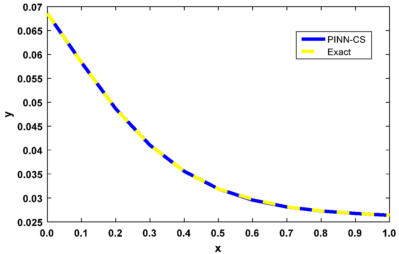
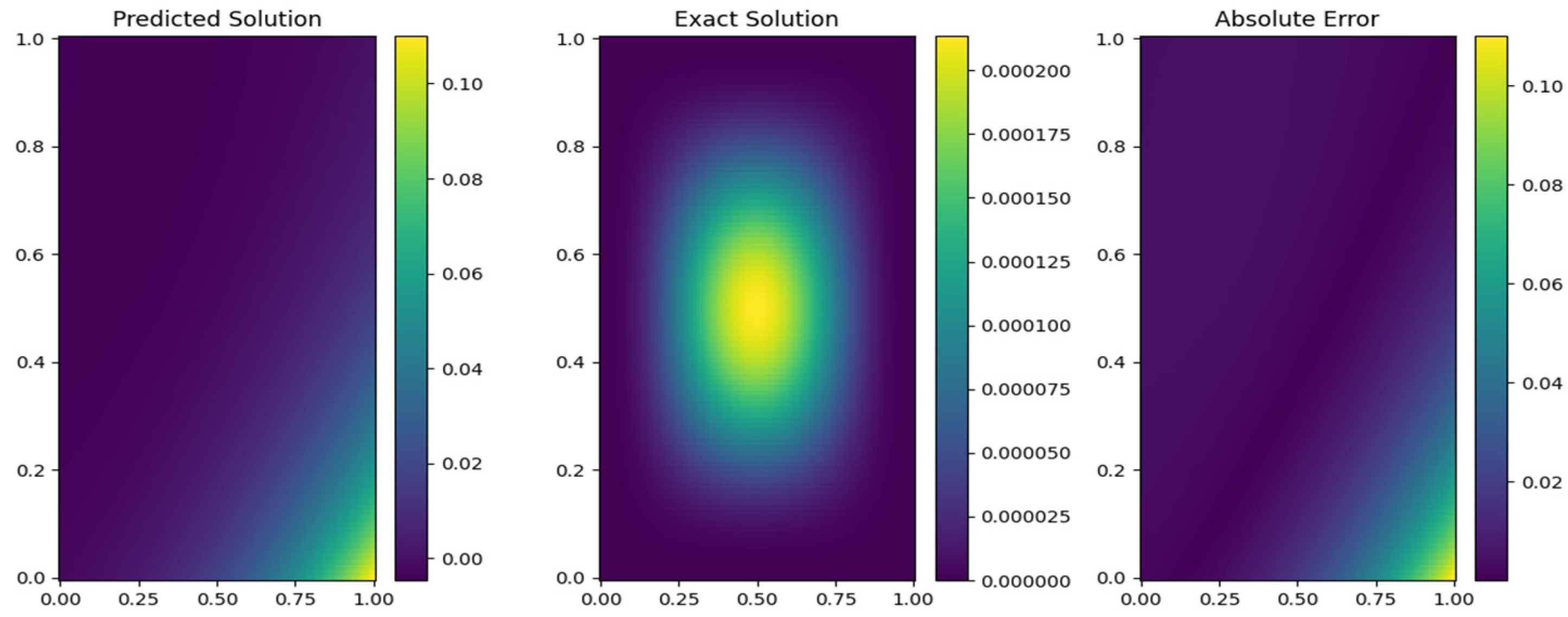
Figure 2 visually compares the numerical solution obtained using the PINN-CS framework with the exact solution for the 2D space-fractional PDE described in Example 1. The overlap between the two solutions is nearly perfect, signifying an extremely high degree of numerical accuracy. The maximum absolute error, as seen in Table 2, is as low as $3.88\times {10}^{-11}$ when $N=8$. This result confirms that PINN-CS provides a highly accurate solution, even with relatively few approximation points. The visual confirmation of the overlap across the domain further reinforces the robustness of the methodology for solving complex fractional PDEs with high precision.

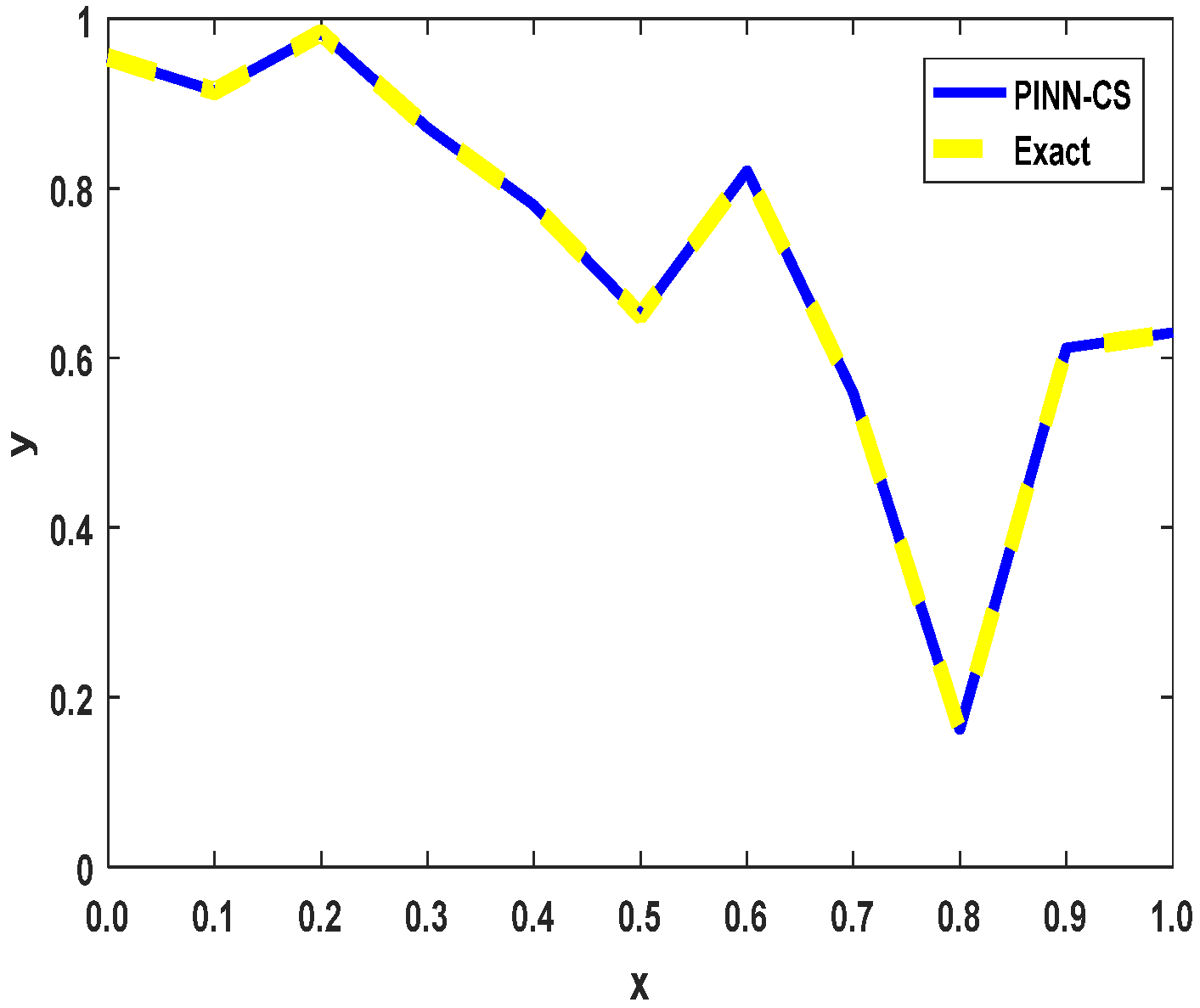
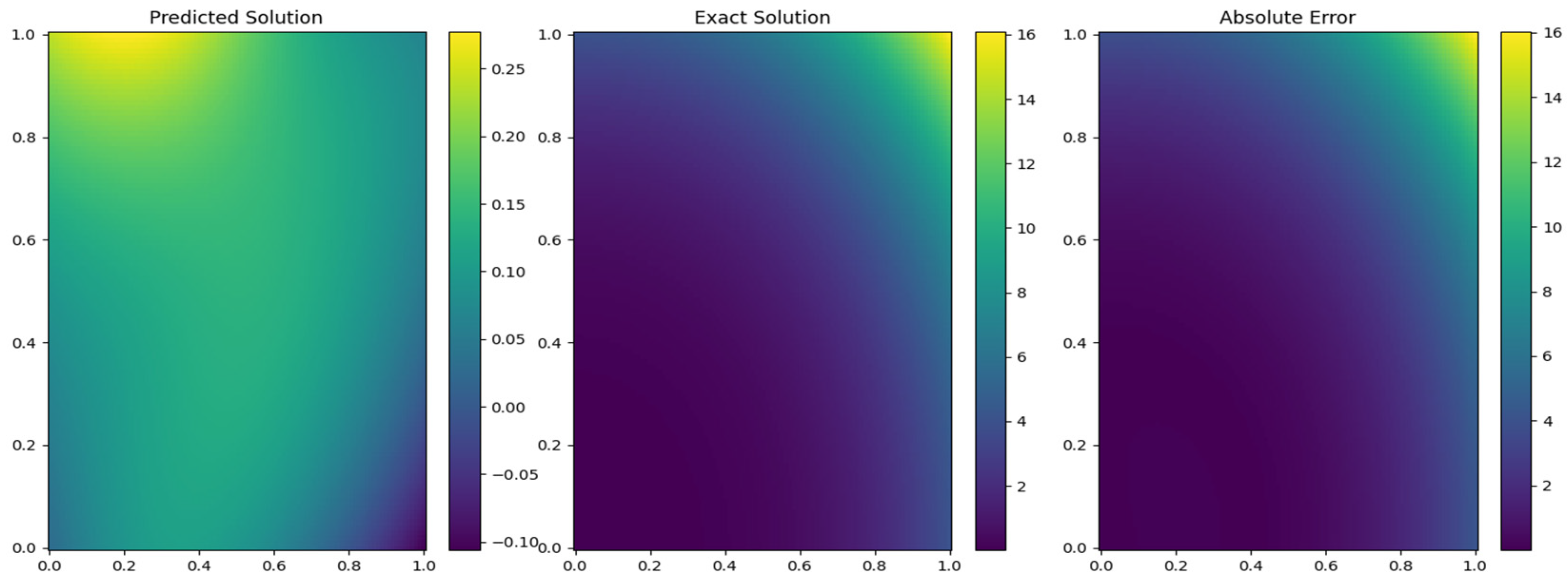
A graphical comparison in Figure 3 shows the overlap between the numerical solution generated by PINN-CS and the exact analytical solution. The solutions overlap almost perfectly, visually confirming the high numerical accuracy reported in Table 5. Wherever such deviations exist, as maintained here, they are minimal and refer to the robust and reliable nature of the underlying PINN-CS framework. This near-perfect level of alignment establishes it as particularly capable of accurately approximating solutions to fractional PDEs.

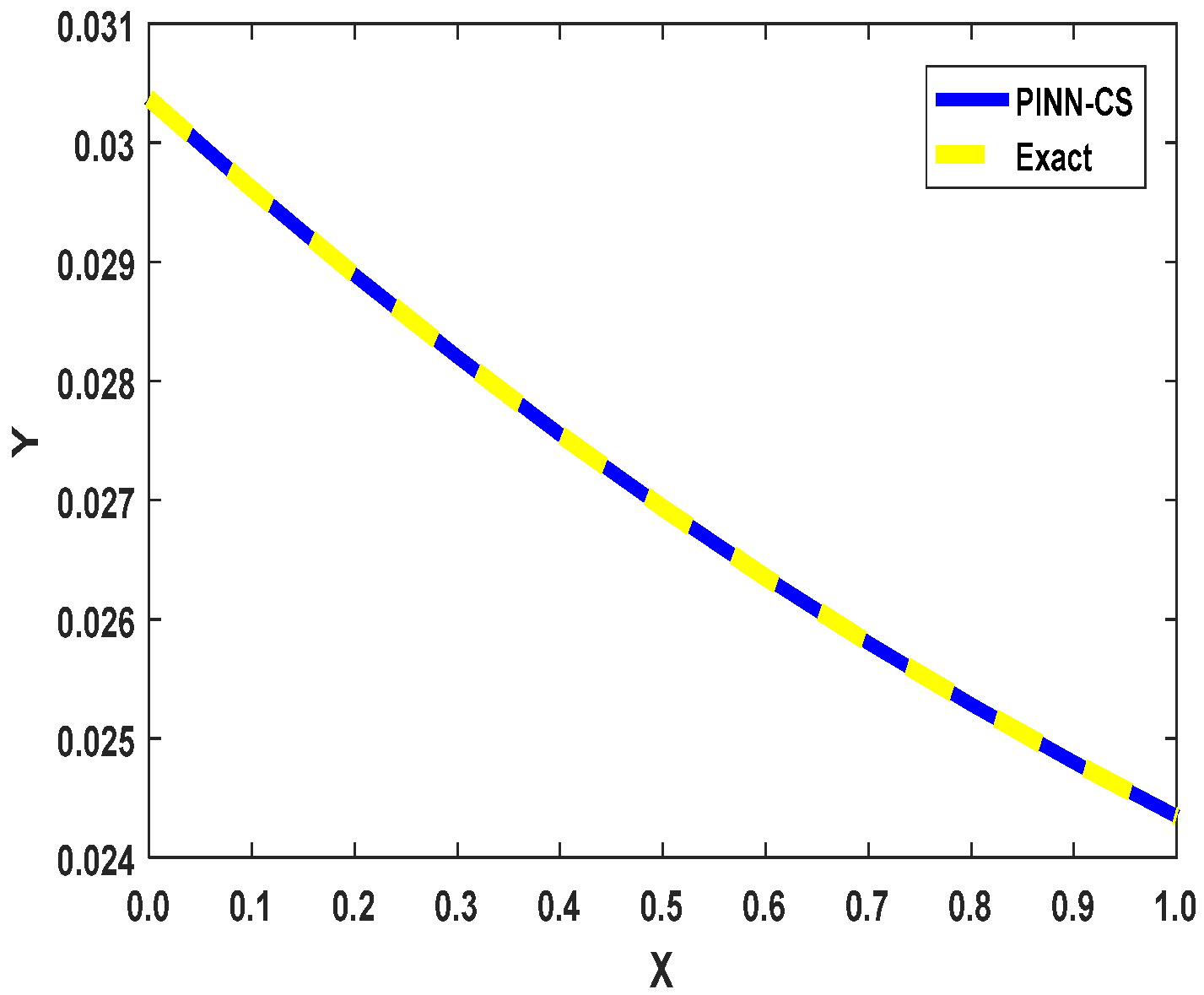
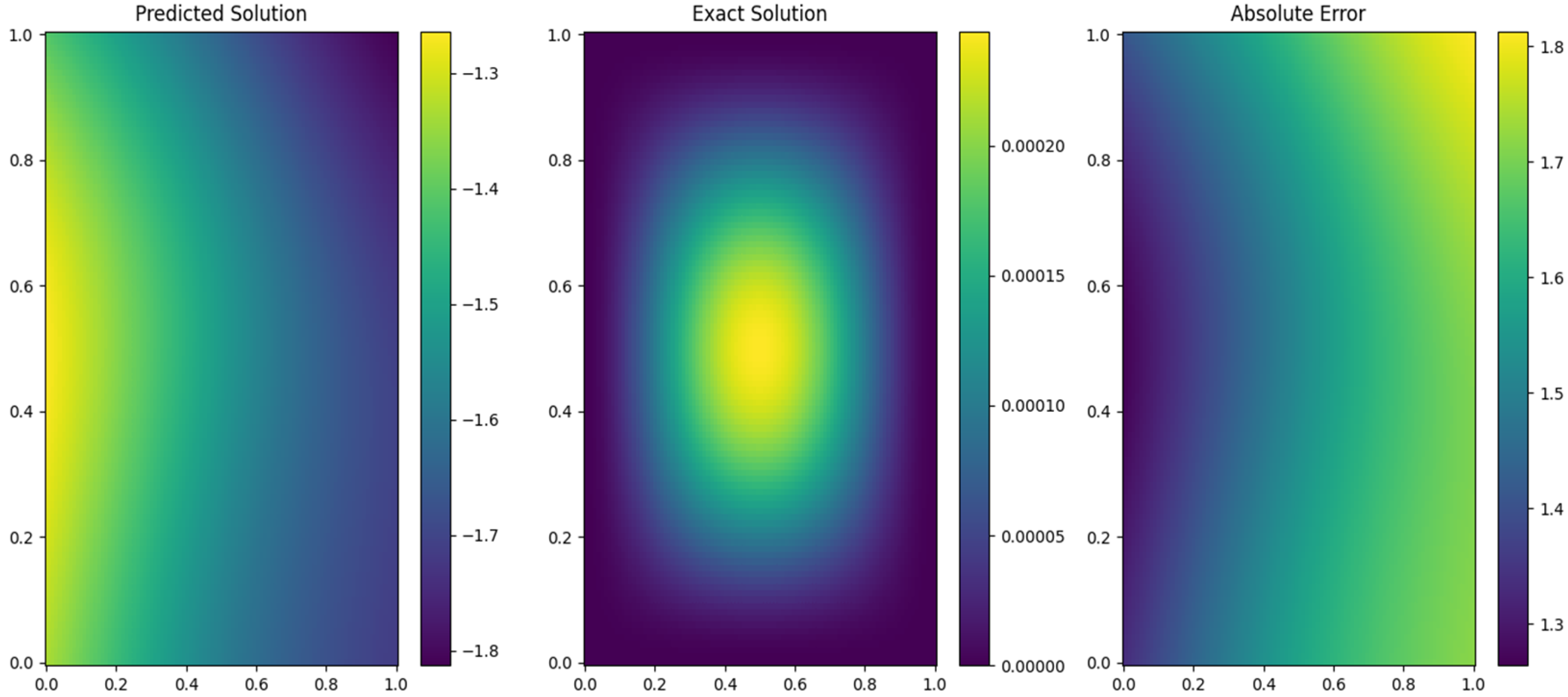
Figure 4 in the paper provides a performance assessment of the PINN-CS framework based on the overlap with the exact solutions to a 3D time-space fractional Bloch–Torrey equation explored in Example 3. The figure shows a good correlation with the loss function obtained with numeric solution given by PINN-CS with the exact analytical solution. The almost complete alignment proves the effectiveness of the PINN-CS approach as an accurate modeling technique. The considered analysis Example 3 is an example of 3D fractional PDE, which makes this problem particularly difficult due to the high dimensionality of the problem and the use of fractional operators. As seen from the solution of this problem, the proposed PINN-CS framework appears sufficiently stable and versatile for dealing with all these kinds of equations. The figure supplements the numerical results described in the table presented in the article, which shows minimal absolute errors calculated for various approximation points. The reported error, being of the order of 10⁻⁴, establishes the high accuracy of the proposed PINN-CS framework further. In Figure 4, the performance of the PINN-CS framework is demonstrated when solving the 3D time-space fractional Bloch–Torrey equation considered in Example 3. This figure also corroborates well with the fact that the PINN-CS method provides a numerical solution very close to the exact analytical solution. This convergence confirms the ability and credibility of the PINN-CS framework in solving intricate high-dimensional fractional partial differential equations (fPDEs).

Figure 5 plots a quantitative solution of PINN-CS with the exact analytical solution for the 3D Bloch–Torrey equations. The coincidence of the locations of the solutions to both carriers is almost perfect, which proves a high accuracy in the formulation of the PINN-CS framework. This figure shows that PINN-CS has the ability to approximate the dynamics of high-dimensional fractional PDEs. The minimal deviations corroborate the low absolute errors reported, validating the framework’s reliability for applications requiring precise numerical approximations.

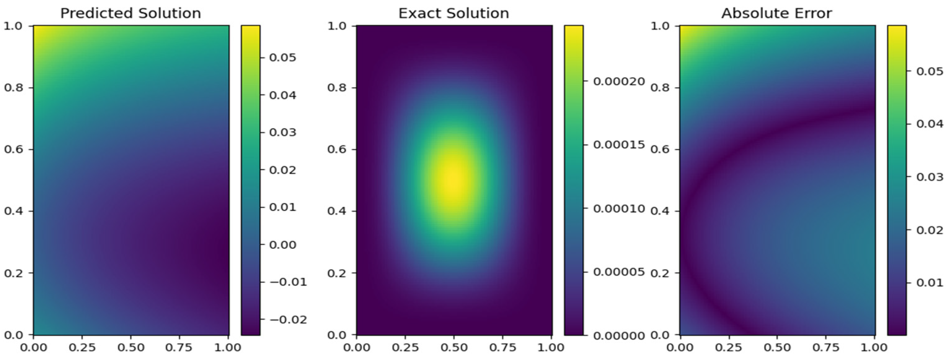
Figure 6 shows the point-wise error distribution as a heatmap for the 2D space-fractional PDE solved in Example 1. The errors are minimal across the domain, with most values concentrated in the range of ${10}^{-11}$ to ${10}^{-9}$, as corroborated by the numerical results in Table 2. While the errors are uniformly low, minor peaks near the boundary regions highlight areas where further refinement may marginally enhance accuracy. The figure underscores the efficacy of the PINN-CS framework, achieving a point-wise error that is orders of magnitude smaller than the competing methods, such as Monte Carlo fPINN $\left(2.91\times {10}^{-1}\right.$ at $N=8$) and traditional fPINN $(3.73\times$ ${10}^{-1}$ at $N=8$).

Figure 7 illustrates the point-wise error distribution across the computational domain as a heatmap. The errors are minimal, mostly concentrated in the range of ${10}^{-9}$ to ${10}^{-8}$, with slight peaks near boundary regions. The consistency of the error distribution clearly shows that the PINN-CS framework has good accuracy over the whole domain. Small humps arise around the edges of the plot, suggesting areas where precision might be further improved by additional refinement of the data. This shows the relevance of node distribution in the consideration of boundary effects.

The point-wise error distribution in Figure 8 in the paper is implemented for the 3D time-space fractional Bloch–Torrey equations for evaluating the efficiency of the physics-informed neural network coupled with the cuckoo search algorithm, called PINN-CS. The heatmap in Figure 8 specifies that there exists minimal standard error spread wide and far across the computational domain, with most evaluations clustered closely to the range of ${10}^{-9}$ to ${10}^{-8}$. This observation This further demonstrates the fractal precision of the PINN-CS methodology in solving difficult equations in a shorter CPU time. An additional interesting aspect can be revealed by looking closely at how the errors are distributed, which is the slight increase in the values of the errors during the approach toward the bounds of the computational domain. These peaks can be attributed to the challenges related to approximating boundary conditions in high-dimensional fractional systems. The phenomenon of boundary effects points to certain directions for improvement with regard to sampling techniques or improved management of boundary conditions.

Finally, the heat map shown in Figure 9 represents the point-wise error distribution for the 3D Bloch–Torrey equations. As shown here, all the errors are bounded and spread out evenly throughout the computational domain with dominant values between 10⁻⁸ and 10⁻⁹. Defective scores, which are slightly higher near the boundaries, indicate scope for increase in efficacy concerning the handling aspects of boundaries. This figure strengthens the PINN-CS framework to hold high accuracy in the domain and provide the ability to solve complicated fractional PDEs.

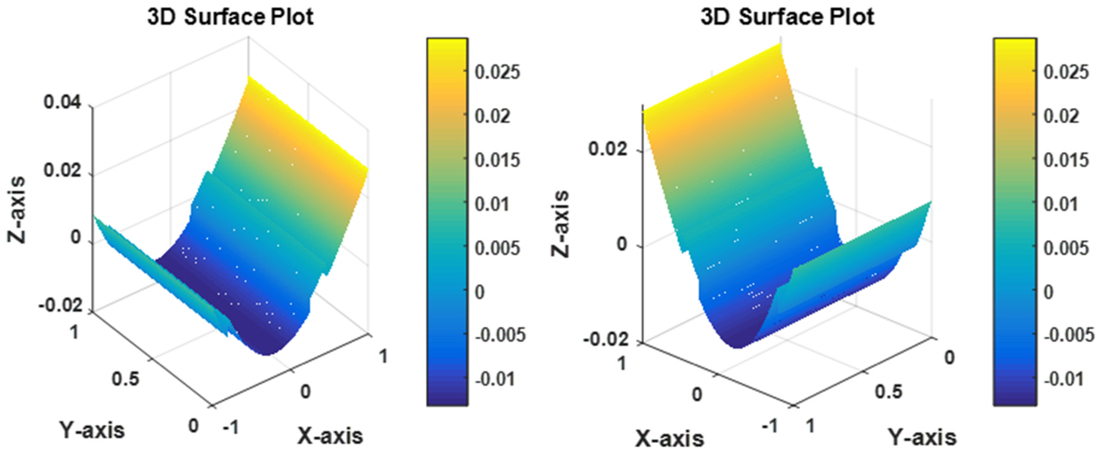
The PINN-CS solution of the 2D space-fractional PDE is presented by the 3D surface plot in Figure 10. This figure presents the numerical results in which it is observed that the solution surface is continuous and smooth and is in good agreement with the exact solution. The low point-wise errors ($\sim {10}^{-10}$ for $N=128$) ensure the solution’s accuracy across the domain. Here, this graphical representation demonstrates the ability of the PINN-CS framework to predict several behaviors of fractional PDEs in terms of accuracy as well as to address high-dimensional problems in more complicated areas. The solution presented below is visually more coherent and accurate, further strengthening the architecture of the proposed framework.

Table 4. Shows the parameter setting for Example 3.2 (2D time-space fractional diffusion).

Parameter	Value
$\mathrm{Approximate} \mathrm{point} N$	100
Hidden layers	4
Neurons	5
Activation function	tanh
Optimizer	Cuckoo Search Algorithm
Number of iterations	1000
$\alpha$	0.3
$\beta$	1.7

provides parameter settings for Example 2, which involves solving a 2D time-space fractional diffusion equation. The parameters contain 100 approximate points, which represent the number of approximation points utilised in numerical computation. The four hidden layers represent the depth of the neural network architecture. Each layer has five neurones, which determines the neural network’s complexity. The activation function is $tanh$, chosen for its smooth and differentiable nature, suitable for physics-informed neural networks. The optimizer is the cuckoo search algorithm, employed for tuning parameters efficiently. The number of iterations is set to 1000, ensuring adequate optimization steps for convergence. The fractional orders $\alpha =0.3$ and $\beta =1.7$ highlight the characteristics of the diffusion process in the time and spatial domains, respectively.

Example 2.

We move forward by examining the following 2D time-space fractional diffusion equation, along with its initial and boundary conditions, within three distinct regions ${\mathrm{\Omega }}_1$.

$$\begin{array}{ll}{}_0{}^{c}D_t^{\alpha }u(x,y,t)& =-K_1(-\mathsf{\Delta }{)}_{xx}^{{\beta }_1}u(x,y,t)-K_2(-△{)}_{yy}^{{\beta }_2}u(x,y,t)\\ & +f(x,y,t),(x,y,t)\in {\mathrm{\Omega }}_i\times (0,T]\end{array},$$

(41)

with the initial conditions:

$$u\left(x,y,0\right)=u_0\left(x,y\right),\left(x,y\right)\in {\mathrm{\Omega }}_i,$$

(42)

with the boundary condition:

$$u(x,y,t)=0,(x,y)\in \partial {\mathrm{\Omega }}_i\times (0,T].$$

(43)

The exact solution considered for the above problem is given by:

$$u\left(x, y, t\right)={(x-x_{lb})}^3{(x_{ub}-x)}^3{(y-y_{lb})}^3{(y_{ub}-y)}^3\cos (t).$$

(44)

Given this exact solution, the forcing term f (x, y, t) can be expressed as:

$$f(x,y,t)=f_1(x,y,t)+f_2(x,y,t)+f_3(x,y,t).$$

(45)

where $f_1(x,y,t),f_2(x,y,t),$ and $f_3(x,y,t)$ are expressed as:

$$f_1(x, y, t)={(x-x_{lb})}^3{(x_{ub}-x)}^3{(y-y_{lb})}^3{(y_{ub}-y)}^3\cos (t+{\displaystyle \frac{\mathrm{п}\alpha }{2}}),$$

(46)

$$\begin{array}{ll}{f}_2(x,y,t)& ={\displaystyle \frac{1}{2\mathrm{c}\mathrm{o}\mathrm{s}(\pi \alpha /2)}}\left\{{\displaystyle \frac{{\left|x_{lb}+x_{ub}\right|}^3\Gamma (4)}{\Gamma (4-\alpha )}}\left({\left(x-x_{lb}\right)}^{3-\alpha }+{\left(x_{ub}-x\right)}^{3-\alpha }\right)\right.\\ & -{\displaystyle \frac{3{\left|x_{lb}+x_{ub}\right|}^2\Gamma (5)}{\Gamma (5-\alpha )}}\left({\left(x-x_{lb}\right)}^{4-\alpha }+{\left(x_{ub}-x\right)}^{4-\alpha }\right)\\ & +{\displaystyle \frac{3\left|x_{lb}+x_{ub}\right|\Gamma (6)}{\Gamma (6-\alpha )}}\left({\left(x-x_{lb}\right)}^{5-\alpha }+{\left(x_{ub}-x\right)}^{5-\alpha }\right)\\ & \left.-{\displaystyle \frac{3\Gamma \left(7\right)}{\Gamma \left(7-\alpha \right)}}\left({\left(x-x_{lb}\right)}^{6-\alpha }+{\left(x_{ub}-x\right)}^{6-\alpha }\right)\right\}{\left(y-y_{lb}\right)}^3{\left(y_{ub}-y\right)}^3\cos (t),\end{array}$$

(47)

$$\begin{array}{ll}{f}_3(x,y,t)& ={\displaystyle \frac{1}{2\mathrm{c}\mathrm{o}\mathrm{s}(\pi \beta /2)}}\left\{{\displaystyle \frac{{\left|y_{lb}+y_{ub}\right|}^3\Gamma (4)}{\Gamma (4-\beta )}}\left({\left(y-y_{lb}\right)}^{3-\beta }+{\left(y_{ub}-y\right)}^{3-\beta }\right)\right.\\ & -{\displaystyle \frac{3{\left|y_{lb}+y_{ub}\right|}^2\Gamma (5)}{\Gamma (5-\beta )}}\left({\left(y-y_{lb}\right)}^{4-\beta }+{\left(y_{ub}-y\right)}^{4-\beta }\right)\\ & +{\displaystyle \frac{3\left|y_{lb}+y_{ub}\right|\Gamma (6)}{\Gamma (6-\beta )}}\left({\left(y-y_{lb}\right)}^{5-\beta }+{\left(y_{ub}-y\right)}^{5-\beta }\right)\\ & \left.-{\displaystyle \frac{3\Gamma \left(7\right)}{\Gamma \left(7-\beta \right)}}\left({\left(y-y_{lb}\right)}^{6-\beta }+{\left(y_{ub}-y\right)}^{6-\beta }\right)\right\}{\left(x-x_{lb}\right)}^3{\left(x_{ub}-x\right)}^3\cos (t).\end{array}$$

(48)

For the sake of simplicity, we will assume $K_1$$=1,K_2=1,$ and $T=1$. The Table 4 shows the parameter setting for the 2D time-space fractional diffusion equation. Example 2 focuses on solving a 2D time-space fractional diffusion equation using the proposed PINN-CS framework. The governing equation is characterized by fractional orders $\alpha =0.3$ (time) and $\beta =1.7$ (space), reflecting the non-local temporal and spatial dynamics inherent in fractional systems. The problem includes specified initial and boundary conditions over a given domain, with the exact solution provided for validation purposes.

Table 5. Comparison of performance between fPINN [29], Monte Carlo PINN, and PINN-CS methods (2D time-space fractional diffusion equation) on Ω1 for Example 2, for α = 0.3, β = 1.7.

N	fPINN	Monte Carlo PINN	PINN-CS
$20$	$5.79\times 10$−1	$2.59\times 10$−1	$3.26\times 10$−9
$40$	$8.98\times 10$−2	$7.64\times 10$−2	$1.19\times 10$−8
$80$	$4.11\times 10$−2	$4.01\times 10$−2	$3.67\times 10$−9

provides a comparative analysis of the numerical performance of three methods—fPINN, Monte Carlo fPINN, and the proposed PINN-CS framework—when applied to a 2D time-space fractional diffusion equation. The comparison is based on different values of $N$, the number of approximation points, for fractional orders $\alpha =0.3$ and $\beta =1.7$. It is observed that fPINN shows relatively lower accuracy, with the error remaining in the range of ${10}^{-1}$ even at higher approximation points. Monte Carlo fPINN improves upon fPINN by using Monte Carlo techniques, achieving errors in the order of ${10}^{-2}$ for larger $N$. On the other hand, PINN-CS outperforms both, with errors consistently in the range of ${10}^{-8}$ to ${10}^{-9}$ across all $N$, demonstrating a dramatic improvement in accuracy. Across all methods, increasing $N$ leads to lower errors, indicating improved numerical resolution. However, the rate of improvement is most pronounced in the PINN-CS framework, showcasing its superior ability to handle high-dimensional fractional PDEs. Moreover, at $N=128$, the error for fPINN remains significantly higher compared to PINN-CS, with a difference of several orders of magnitude. This highlights the enhanced precision of the PINN-CS approach, particularly in capturing the complexities of fractional diffusion equations.

Table 6. Time complexity of different methods for Example 2.

N	fPINN Time to Run Ten Iterations	Monte Carlo PINN Time to Run Ten Iterations	PINN-CS Time to Run Ten Iterations
$\mathbf{20}$	$0.09$	$0.05$	$0.08$
$\mathbf{40}$	$0.13$	$0.07$	$0.14$
$\mathbf{80}$	$0.24$	$0.13$	$0.21$

illustrates the time complexity of fPINN, Monte Carlo PINN, and PINN-CS by recording the time taken for ten iterations at different values of NN. As expected, the computation time increases with NN for all the methods. Monte Carlo PINN consistently demonstrates the fastest performance, particularly for larger values of NN, indicating its computational efficiency. While fPINN and PINN-CS show relatively close performance, their runtime fluctuates slightly depending on NN. The results suggest that Monte Carlo PINN is the most efficient among the three methods, making it a suitable choice for scenarios where minimizing computation time is a priority.

Figure 11 shows a 3D graphical representation of the solution for Example 2, where a 2D time-space fractional diffusion equation is solved using the proposed PINN-CS framework. The figure further clearly expresses the rapid and concise character of the solution and guarantees that the method is capable of capturing all the performances of the fPDEs within the computational domain. In the 3D surface plot, one can observe the numerical solution that has been developed in the PINN-CS framework while maintaining continuous and accurate forms in all structures found in the domain. This is particularly important because PINN-CS is able to model the fractional dynamics, such as time and space, which are given in the governing equations. The positioning of the solution to the expected physical behavior in graphical form gives qualitative assurance of the strength of the method. The figure also demonstrates the ability of the PINN-CS approach to operate in high-dimensional spaces and address the issues with the boundary conditions discussed in Example 2.

Table 7. This shows the parameter settings for Example 3 (3D time-space fractional Bloch–Torrey equation).

Parameter	Value	Parameter	Value
Approximate point N	$100$	Neurons	5
Hidden layer	$4$	Activation function	$tanh$
Optimizer	Cuckoo Search algorithm	Number of iterations	1000
α	$1.9$	β	1.5
$K1, k2$	$1$	$r$	0.5

provides the specific parameter settings utilized for solving the 3D time-space fractional Bloch–Torrey equation (Example 3) using the PINN-CS (physics-informed neural networks integrated with cuckoo search) framework.

Example 3.

This examines the 3D time-space fractional Bloch–Torrey equation defined within a spherical domain Ω = (x, y, z):$\sqrt{x^2+y^2+z^2}$< r = 1/2 considering the homogeneous initial and boundary conditions [39].

$$\begin{gathered} {K_{\mathrm{\alpha }}}^{\mathrm{C}}{D^{\mathrm{\alpha }}}_{\mathrm{t}}u(x,y,z,t)=K_{\mathrm{\beta }}{R}^{2\mathrm{\beta }}u(x,y,z,t)+f(x,y,z,t), \\ u(x,y,z,0)=0,(x,y,z)\in \Omega , \\ (x,y,z,t)=0,(x,y,z,t)\in R^3\Omega \times (0,T], \end{gathered}$$

(49)

where

$$R^{2\mathrm{\beta }}:={}^{\mathrm{Rz}}D^{{2\mathrm{\beta }}_{\mathrm{x}}}+{}^{\mathrm{Rz}}D^{{2\mathrm{\beta }}_{\mathrm{y}}}+{}^{\mathrm{Rz}}D^{{2\mathrm{\beta }}_{\mathrm{z}}},$$

(50)

where${}^{\mathit{Rz}}D^{{2\beta }_x}$is the Riesz fractional derivative operator,

$${}^{\mathrm{Rz}}D^{{2\mathrm{\beta }}_{\mathrm{x}}}f(x):={\displaystyle \frac{-1}{2cos(\pi \beta )}}(\mathrm{xlb}{D}^{{2\mathrm{\beta }}_{\mathrm{x}}}f(x)+x{D}^{2\mathrm{\beta }}{x}_{\mathrm{ub}}f(x)).$$

(51)

where

• $x_{ib}{D}_x^{2\beta }f(x)$ is the left-sided Riemann–Liouville fractional derivative of order $2\beta$,
• ${}_{x}D_{x_m}^{2\beta }f(x)$ is the right-sided Riemann–Liouville fractional derivative of order $2\beta$,
• $x_{lb}$ and $x_{ub}$ are the lower and upper bounds for the domain of $x$,
• $cos(\pi \beta )$ is a normalization factor to ensure symmetry.

The exact solution of the given problem is:

$$u(x,y,z,t)=2^4{t}^2{(x^2+y^2+z^2-r^2)}^2.$$

(52)

The forcing term of the above problem can be expressed as:

$$\begin{gathered} f(x,y,z,t)=\mathrm{h} (\mathrm{x}, \sqrt{r^2-y^2-z^2})+\mathrm{h} (\mathrm{y}, \sqrt{r^2-x^2-z^2})+\mathrm{h} (\mathrm{z}, \sqrt{r^2-x^2-y^2}) \\ +{\displaystyle \frac{32k_{\alpha }}{\mathrm{┌}(3-\alpha )}}{t}^{2-\mathrm{\alpha }}{(x^2+y^2+z^2-r^2)}^2, \end{gathered}$$

(53)

with

$$\begin{array}{l}h(x,s)={\displaystyle \frac{8K_{\beta t^2}}{cos(\frac{\beta \pi }{2})}}({\displaystyle \frac{8s^2}{\mathrm{┌}(3-2\beta )}}({(x+s)}^{2-\mathrm{\beta }}+{(s-x)}^{2-2\mathrm{\beta }})-{\displaystyle \frac{24s}{\mathrm{┌}(4-2\beta )}}({(x+s)}^{3-2\mathrm{\beta }}+{(s-x)}^{3-2\mathrm{\beta }})\\ +{\displaystyle \frac{24s}{\mathrm{┌}(5-2\beta )}}({(x+s)}^{4-2\mathrm{\beta }}+{(s-x)}^{4-2\mathrm{\beta }},\end{array}$$

(54)

For simplicity, we take K_α = 1, K_β = 1, and T = 1.

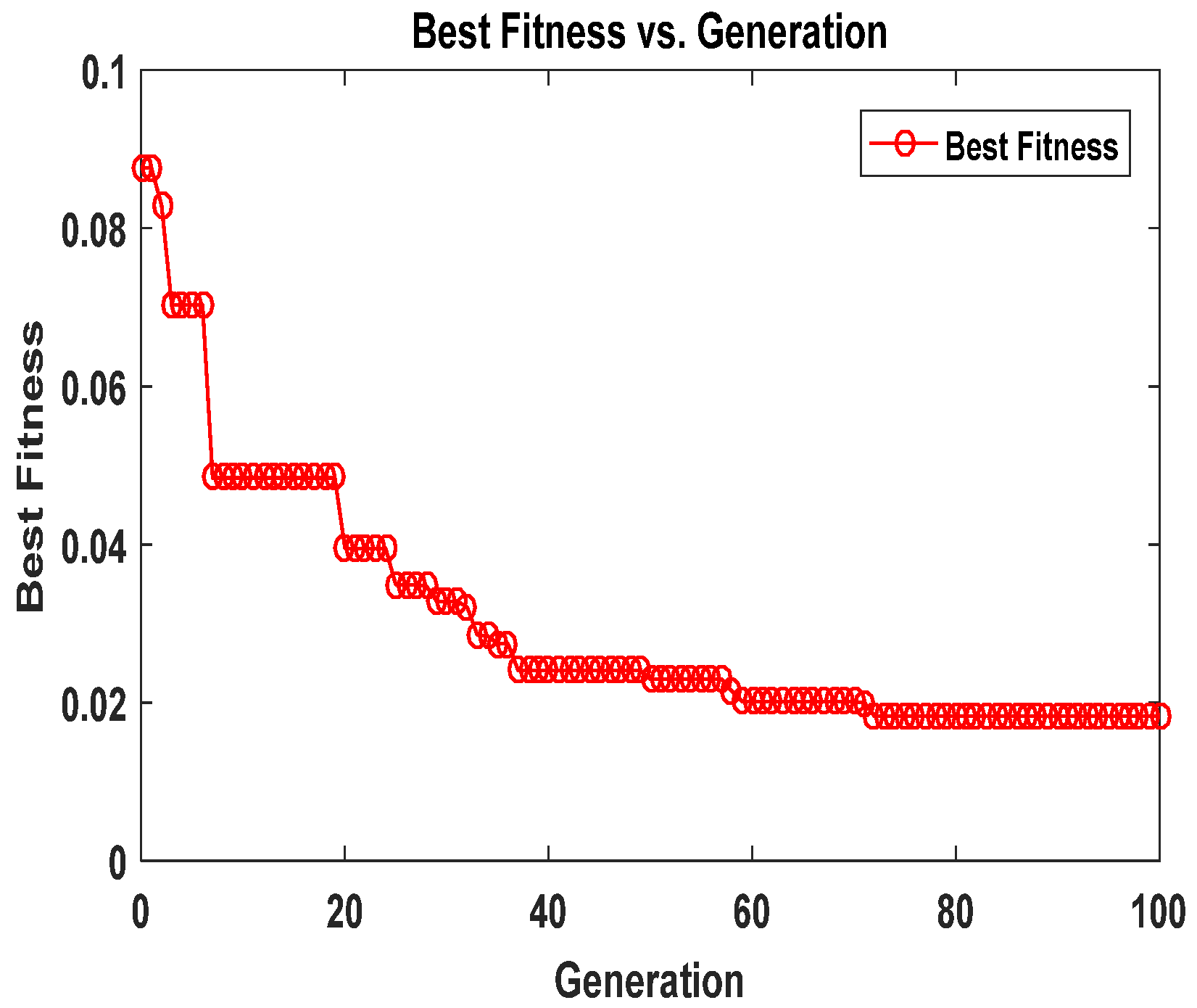
Figure 12 tracks the evolution of the best fitness value during the cuckoo search (CS) optimization. The initial fitness value starts relatively high, reflecting the significant discrepancy between the initial model parameters and the exact solution. However, the fitness rapidly decreases over the first 200 generations, indicating quick convergence of the CS algorithm. Beyond 500 generations, the fitness value plateaus, stabilizing near its optimal value. The consistent improvement in fitness across generations demonstrates the effectiveness of the CS algorithm in optimizing the neural network’s parameters to minimize the loss function and adhere to the governing equations.

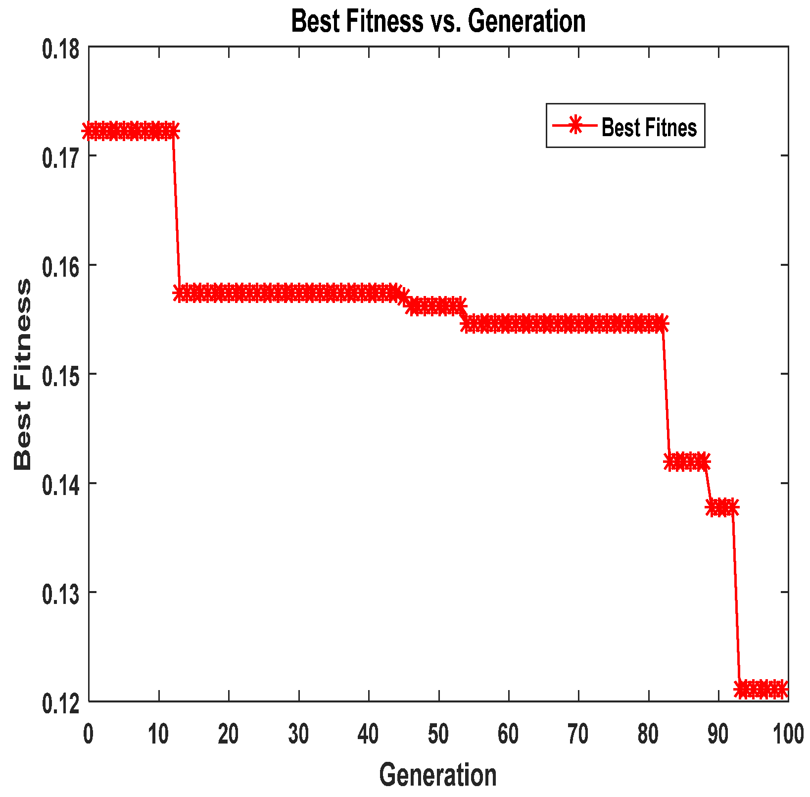
Figure 13 depicts the best fitness value versus the number of generations for the 2D time-space fractional diffusion equations in Example 2. The graph acts as a performance indicator of the optimization implemented in the PINN-CS framework utilizing the CS optimization algorithm for adjusting the parameters of the neural network. The fitness value begins with a reasonably high value, suggesting a large gap between the preliminary predictions of the neural network and the exact solutions. The fitness value falls sharply during early generations, or at least the initial 200 generations as shown below. This is in concordance with the ability of the CS algorithm to improve the parameters’ values at a faster rate compared to the rate of decrease in the loss function.

After 500 generations, the fitness curve levels off, indicating that the algorithm has likely reached an optimal or near-optimal solution. The steady improvement in fitness values reflects the effectiveness of the CS algorithm in optimizing the neural network parameters. This ensures that the approximated solutions align well with the governing equations of the fractional diffusion problem. The fast convergence underscores the computational efficiency of the PINN-CS framework, making it a practical and powerful tool for addressing complex fractional partial differential equations.

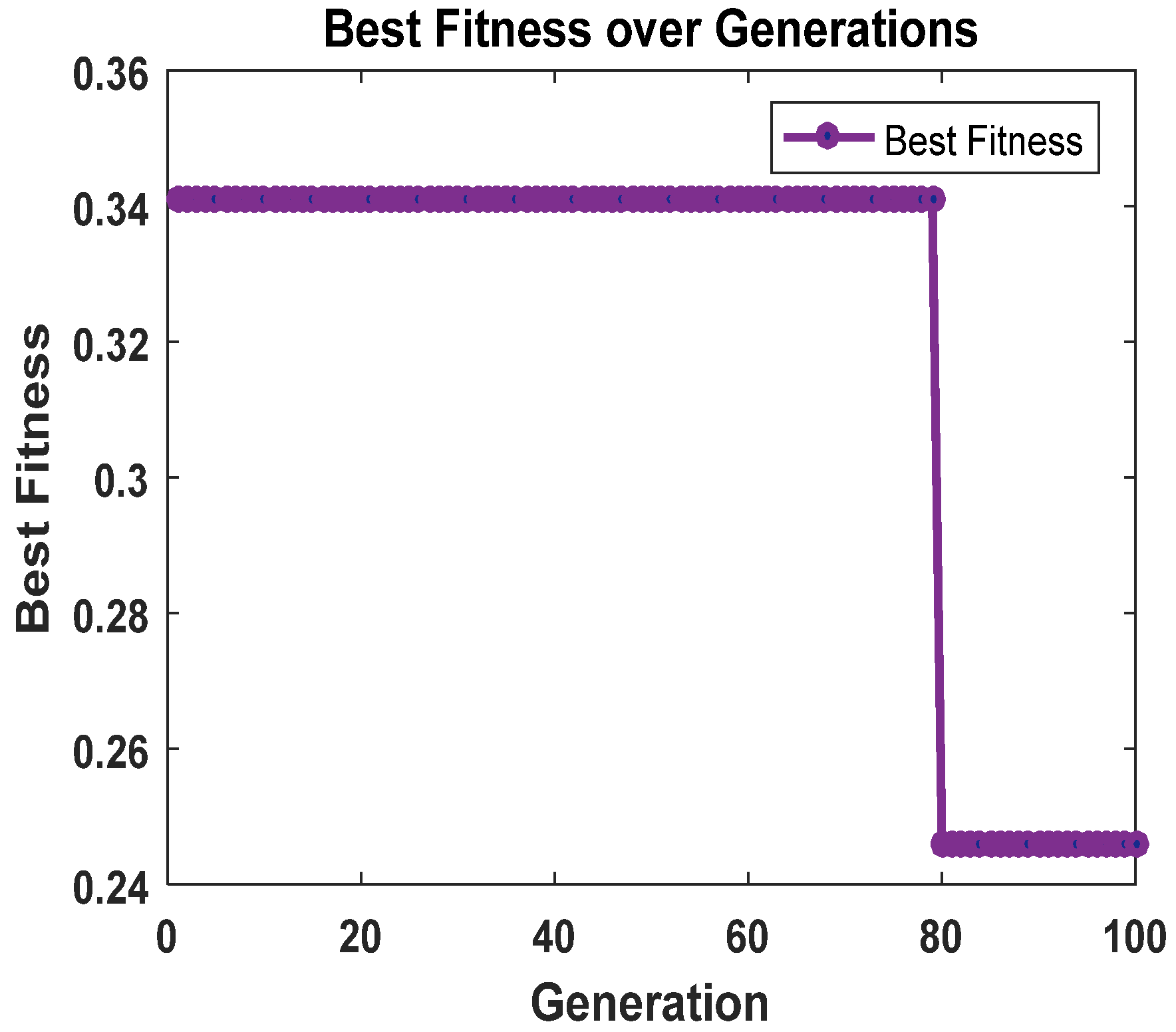
Figure 14 tracks the evolution of the best fitness value during the optimization process for the 3D Bloch–Torrey equation. The fitness starts greatly, as the initial model may be greatly off the true solution. As can be seen here, the dropping is most prominent in the first 200 generations, showing that the cuckoo search algorithm converges very quickly. The fitness value remains constant after 500 generations; this signifies that the evolution process has reached an optimal or a very nearly optimal solution. These results clearly show that the proposed CS algorithm can effectively tune parameters so that the approximated solutions are very close to the derived governing equations.

Figure 15 also presents the convergence graph of the PINN-CS for the 3D Bloch–Torrey equations during the PINN-CS optimization process. Like Figure 14, the fitness value initiates from a high level and drops a great deal in the initial phase, which indicates optimization. After 500 generations, it is observed that the curve starts to level off and approaches the optimal solution. This pattern also suggests that the cuckoo search algorithm is effective for the adjustment of the network parameters in reaching accurate numerical solutions of the PINN-CS architecture.

The solutions furnished by the presented PINN-CS framework for Example 3 are given in

Table 8. This shows the performance of the PINN-CS of the 3D time-space fractional Bloch–Torrey equations of Example 3.

N	PINN-CS	Exact	Absolute Error
$0$	$0.954497$	$0.954394$	$1.03\times 10$−4
$1$	$0.91483$	$0.914722$	$1.07\times 10$−4
$2$	$0.98323$	$0.98311$	$1.20\times 10$−4
$3$	$0.871332$	$0.871188$	$1.44\times 10$−4
$4$	$0.780214$	$0.780034$	$1.80\times 10$−4
$5$	$0.65021$	$0.649977$	$2.33\times 10$−4
$6$	$0.820533$	$0.820227$	$3.06\times 10$−4
$7$	$0.558626$	$0.55822$	$4.06\times 10$−4
$8$	$0.161817$	$0.161278$	$5.39\times 10$−4
$9$	$0.611919$	$0.611207$	$7.12\times 10$−4
$10$	$0.629779$	$0.628845$	$9.34\times 10$−4

. This has been done with the intention of presenting the performance of the proposed PINN-CS method with respect to accuracy and reliability in the table below. The first column is the number of discrete points that have been used in order to compute the numerical solutions. These points refer to the size of the computational domain, where larger values of ‘N’ net a greater level of detail. The second column holds the results, which were obtained using the PINN-CS method. These are the forecasted solutions obtained employing the physics-informed neural network with the cuckoo search optimization technique. The third column presents the solutions to the problem, which are obtained analytically and compared with the PINN-CS results to evaluate the robustness of the PINN-CS models. The fourth column provides the absolute errors, calculated as the difference between the PINN-CS solutions and the exact solutions. These errors quantify the accuracy of the numerical method. The absolute errors reported in the fourth column are consistently negligible across all values of N, indicating that the PINN-CS framework achieves near-perfect agreement with the exact solutions. The low absolute errors demonstrate the computational efficiency of the PINN-CS method.

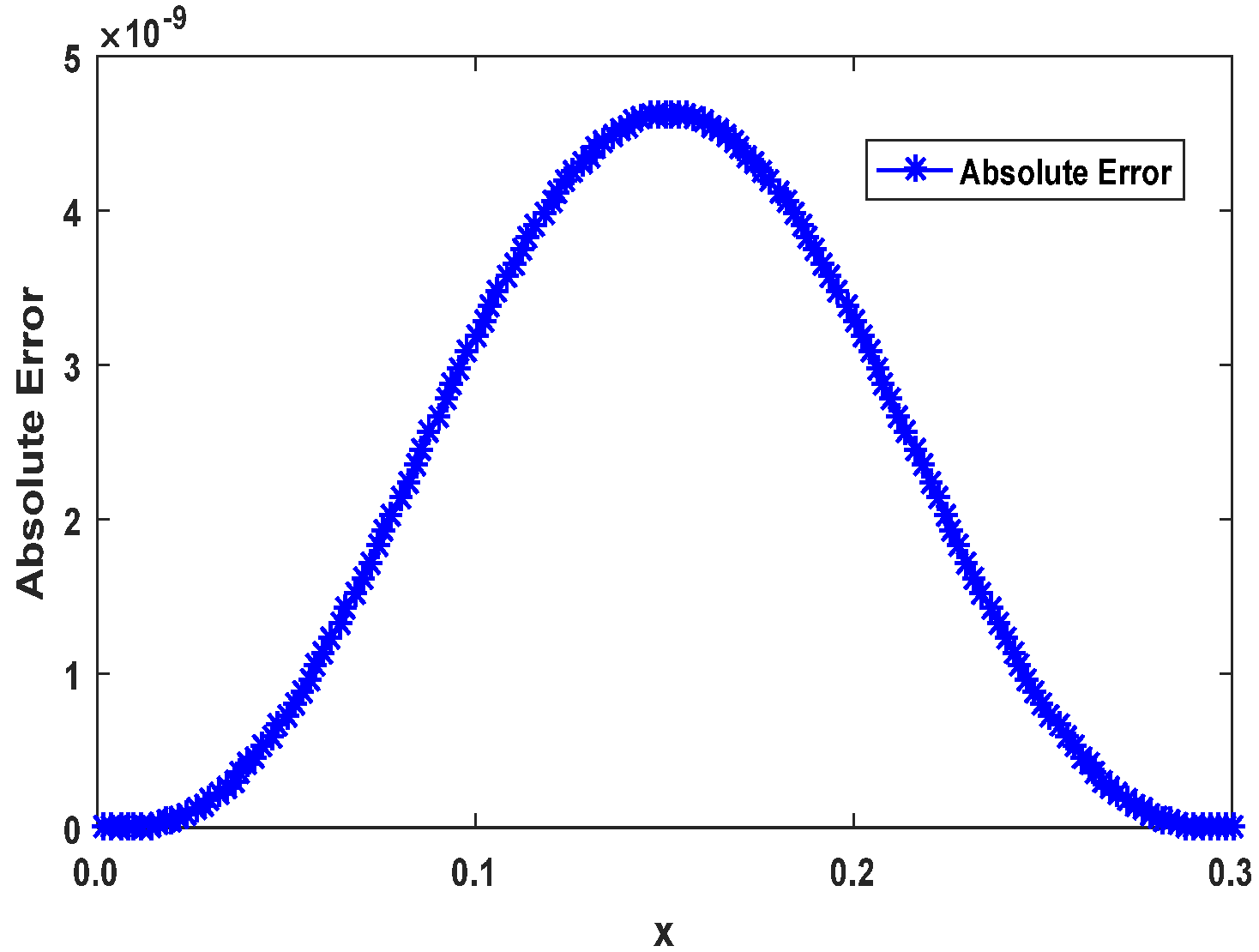
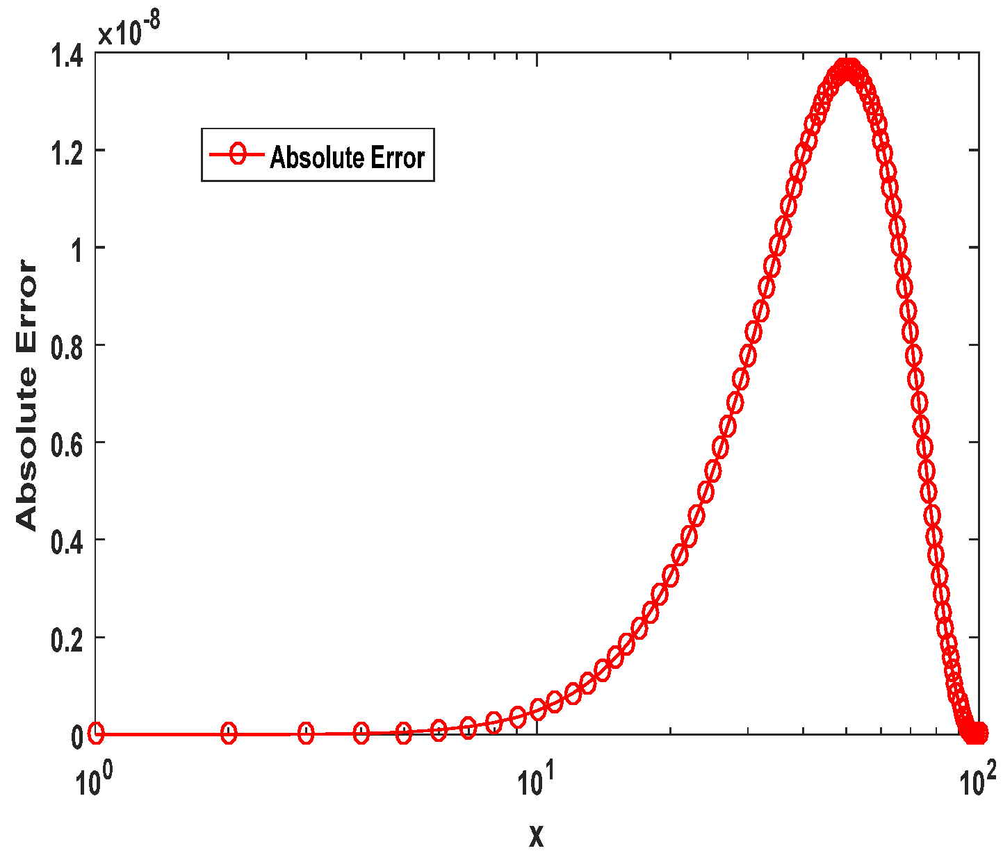
Figure 16 presents the absolute error values for the numerical solution across the computational domain. For $N=128$, the absolute error drops to $5.25\times {10}^{-10}$, as per Table 2. This figure highlights the rapid reduction in error magnitude as the number of points used for approximation grows. The visual representation confirms that PINN-CS consistently outperforms other methods by achieving significantly lower error rates across all resolutions. For example, at $N=$ 32, the PINN-CS error $\left(1.12\times {10}^{-9}\right)$ is orders of magnitude smaller than both Monte Carlo fPINN ($5.97\times {10}^{-2}$) and fPINN $\left(6.71\times {10}^{-2}\right)$.

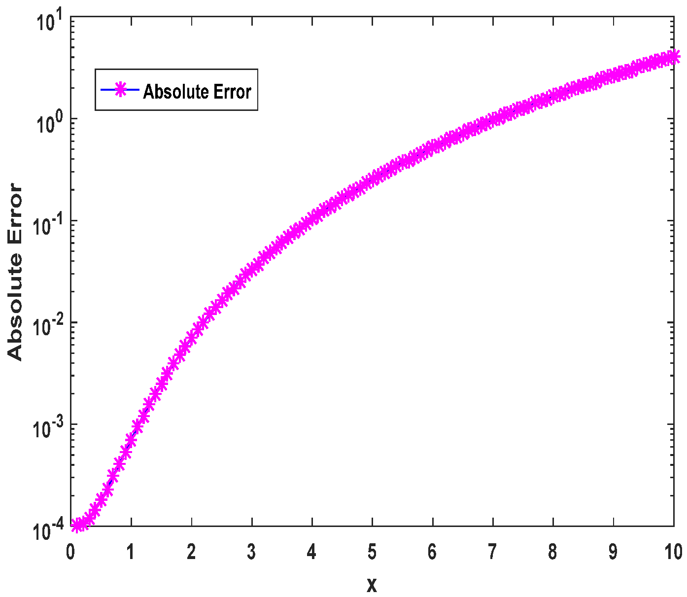
Figure 17 illustrates the absolute errors in solving 2D time-space fractional diffusion equations using the proposed PINN-CS framework for Example 2. From the above graph, a detailed depiction of the distribution of errors throughout the computational domain is well illustrated, showing how PINN-CS overcomes numerical discrepancies. The absolute errors are surprisingly low and that proves again the high accuracy of the proposed PINN-CS approach. For most computational points, the error is in the range of ${10}^{-9}$ to ${10}^{-10}$, significantly outperforming other methods like fPINN and Monte Carlo fPINN. The graph illustrates a steady decrease in error with the increase in approximation points, showcasing the PINN-CS method’s adaptability and reliability for tackling high-dimensional fractional PDEs. Although the overall error remains minimal, minor spikes near the boundaries indicate potential improvements in node placement or boundary condition strategies to boost accuracy. This visualization underscores the PINN-CS framework’s advantage over conventional approaches, excelling in both precision and computational performance.

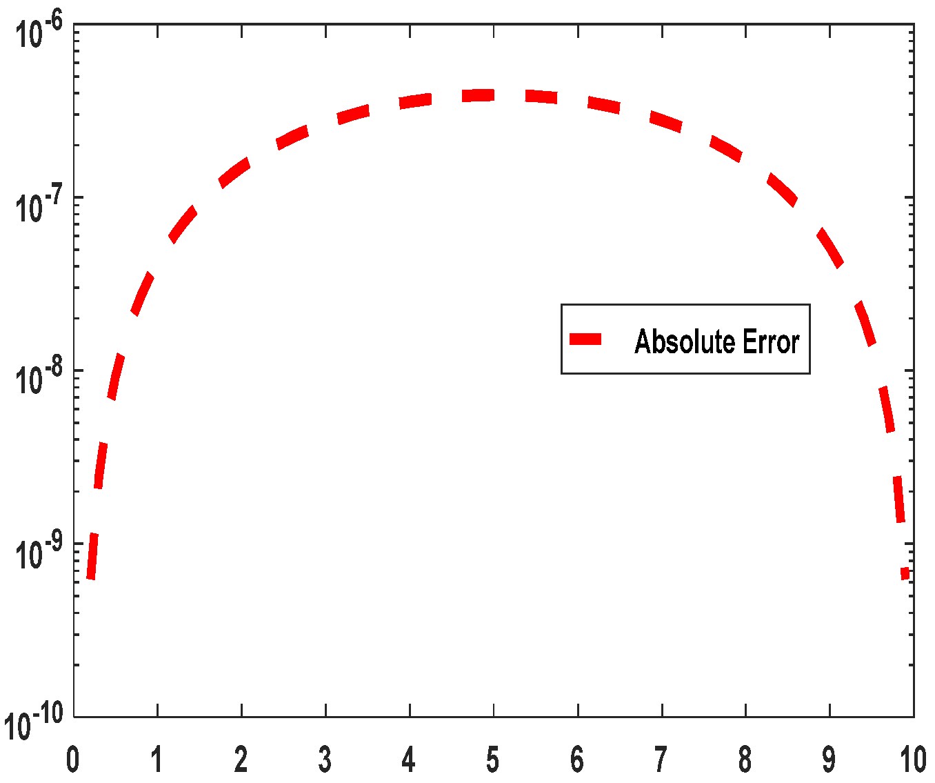
The distribution of the absolute error of the 3D time-space fractional Bloch–Torrey equations solved using the PINN-CS framework is shown in the Figure 18. Their absolute error values are very small in all cases at 10⁻⁸ to 10⁻⁹ and are relatively small across the computational domain. Such uniform distribution shows that the given method is rather accurate and stable. Small fluctuations are noticeable near the boundary areas, likely stemming from the inherent difficulty of precisely approximating boundary conditions in high-dimensional fractional systems. This demonstrates the PINN-CS framework’s capability to achieve remarkable accuracy, confirming its reliability in addressing complex 3D fractional PDEs.

Figure 19 illustrates the absolute error distribution for the 3D time-space fractional Bloch–Torrey equations solved in Example 4. The goal of this figure is to plot the relative error throughout the computational domain as well as demonstrate the performance of the physics-informed neural network combined with the cuckoo search algorithm (PINN-CS). The absolute errors are small and are largely within the order of 10⁻⁹ to 10⁻⁸. Almost equal distribution is noted throughout the domain, which underlines that even though the geometry complexity increases, PINN-CS effectively stays in a low error range throughout the computational space. The error values are also observed to have small fluctuations at both the extremes, which can be explained by the difficulties involved in defining extreme conditions for high-dimensional fractional systems. This warrants further development of the boundary treatment or sampling methods in these areas. Figure 19 serves as compelling evidence of the remarkable accuracy and efficiency of the PINN-CS framework, demonstrating its ability to closely align with the exact solutions. The possible error margin is very low, and this fact underlines the usefulness of the described approach when it concerns practical uses.

Example 4.

The three-term time-space fractional Bloch–Torrey equation in three dimensions on a finite domain is considered [40]:

$$\begin{gathered} K_{{\alpha }_0}{\displaystyle \frac{\partial u\left(x,y,z,t\right)}{\partial t}}+K_{{\alpha }_1}{\displaystyle \frac{{\partial }^{{\alpha }_1}u\left(x,y,z,t\right)}{\partial t^{{\alpha }_1}}}+K_{{\alpha }_2}{\displaystyle \frac{{\partial }^{{\alpha }_2}u\left(x,y,z,t\right)}{\partial t^{{\alpha }_2}}} \\ =K_{\beta }\left({\displaystyle \frac{{\partial }^{\beta }u\left(x,y,z,t\right)}{\partial |x{|}^{\beta }}}+{\displaystyle \frac{{\partial }^{\beta }u\left(x,y,z,t\right)}{\partial |y{|}^{\beta }}}+{\displaystyle \frac{{\partial }^{\beta }u\left(x,y,z,t\right)}{\partial |z{|}^{\beta }}}\right)+ \\ f(x,y,z,t) \left(0\le x\le \mathrm{1,0}\le y\le \mathrm{1,0}\le z\le 1,t\ge 0\right), \end{gathered}$$

(55)

$$f\left(x,y,z,t\right)={\sum }_{i=1}^6 f_i\left(x,y,z,t\right),$$

(56)

$$f_1(x,y,z,t)={\displaystyle \frac{K_{{\alpha }_0}\Gamma \left(3\right)}{\Gamma \left(2\right)}}t{x}^2(1-x{)}^2{y}^2(1-y{)}^2{z}^2(1-z{)}^2,$$

(57)

$$f_2(x,y,z,t)={\displaystyle \frac{K_{{\alpha }_1}\Gamma (3)}{\Gamma \left(3-{\alpha }_1\right)}}{t}^{2-{\alpha }_1}{x}^2(1-x{)}^2{y}^2(1-y{)}^2{z}^2(1-z{)}^2,$$

(58)

$$f_3(x,y,z,t)={\displaystyle \frac{K_{{\alpha }_2}\Gamma \left(3\right)}{\Gamma \left(3-{\alpha }_2\right)}}{t}^{2-{\alpha }_2}{x}^2(1-x{)}^2{y}^2(1-y{)}^2{z}^2(1-z{)}^2 ,$$

(59)

$$\begin{gathered} f_4(x,y,z,t)={\displaystyle \frac{K_{\beta }}{2\mathrm{c}\mathrm{o}\mathrm{s}\left(\frac{\beta \pi }{2}\right)}}{t}^2{y}^2(1-y{)}^2{z}^2(1-z{)}^2\left[{\displaystyle \frac{\Gamma (3)}{\Gamma (3-\beta )}}\left(x^{2-\beta }+(1-x{)}^{2-\beta }\right)\right.\left.+{\displaystyle \frac{\Gamma (5)}{\Gamma (5-\beta )}}\left(x^{4-\beta }+ \\ (1-x{)}^{4-\beta }\right)-{\displaystyle \frac{2\Gamma (4)}{\Gamma (4-\beta )}}\left(x^{3-\beta }+(1-x{)}^{3-\beta }\right)\right], \end{gathered}$$

(60)

$$f_5(x,y,z,t)=f_4(y,x,z,t),f_6(x,y,z,t)=f_4(z,y,x,t).$$

(61)

With the initial boundary conditions:

$$u(x,y,z,0)=├ u(x,y,z,t)┤|\_\Gamma =0.$$

(62)

The analytical solution of the given problem is:

$$u(x,y,z,t)=t^2{x}^2(1-\mathrm{x}{)}^2{y}^2(1-y{)}^2{z}^2(1-z{)}^2.$$

(63)

Table 9. This shows the parameter settings for problem 3.4 of 3D time-space fractional Bloch–Torrey equations.

Parameter	Value	Parameter	Value
Approximate point N	$100$	Neurons	5
Hidden layer	$4$	Activation function	$tanh$
Optimizer	Cuckoo Search algorithm	Number of iterations	1000
$\alpha$0$, \alpha$1$, \alpha$2	$1.0, 0.2, 0.7$	β	1.8
$xlb,xub,ylb,yub,zlb,zub$	$0.1$	$t$	0.5

shows the parameter settings for the three-term time-space fractional Bloch–Torrey equation in 3D in a finite domain.

Table 10. This shows the predicted solution of PINN-CS and the exact solution of 3D Bloch–Torrey equations for Example 4.

N	PINN-CS	Exact Solution	Absolute Error
$0$	$0.030370213$	$0.030370213$	$0$
$1$	$0.029611863$	$0.029611863$	$6.25\times 10$−10
$2$	$0.028889991$	$0.028889989$	$2.45\times 10$−9
$3$	$0.028203346$	$0.02820334$	$5.39\times 10$−9
$4$	$0.027552016$	$0.027552007$	$9.39\times 10$−9
$5$	$0.026935346$	$0.026935332$	$1.44\times 10$−8
$6$	$0.026352458$	$0.026352437$	$2.03\times 10$−8
$7$	$0.025802799$	$0.025802772$	$2.70\times 10$−8
$8$	$0.025285102$	$0.025285068$	$3.45\times 10$−8
$9$	$0.024799831$	$0.024799789$	$4.27\times 10$−8
$10$	$0.02434539$	$0.024345339$	$5.15\times 10$−8

provides a comparison between the predicted solutions generated by the PINN-CS framework (a physics-informed neural network integrated with the cuckoo search algorithm) and the exact solutions for the 3D Bloch–Torrey equations from Example 4. It also includes the absolute errors, offering a detailed assessment of the PINN-CS approach’s accuracy and effectiveness. The solutions predicted by the PINN-CS framework align closely with the exact results for all tested approximation points N. The absolute errors are remarkably low, ranging between 10⁻¹⁰ and 10⁻⁸. This level of precision highlights the reliability of the PINN-CS method in delivering accurate results across the entire computational domain, even as the problem complexity varies.

6. Conclusions

In this study, we introduced a novel framework combining Monte Carlo-based physics-informed neural networks (PINNs) with the cuckoo search (CS) algorithm, referred to as PINN-CS, for efficiently solving fractional partial differential equations (fPDEs). The proposed framework capitalizes on the advantages of applying QMC approaches for approximations of the fractional derivatives and the optimization ability of the CS algorithm to reach high total precision and fast convergence rate. Several numerical simulations were performed, and the algorithm was tested to confirm that the PINN-CS method works for the 2D space-fractional Poisson equations, the 2D time-space fractional diffusion equations, and the 3D time-space fractional Bloch–Torrey equations. The results show that the proposed PINN-CS framework is more accurate and efficient than the fPINN and Monte Carlo fPINN techniques. The usage of the structured sampling nodes and block-sampled approximations saves computer space and reduces computational time considerably. However, the precision of the solution estimate is still high. Furthermore, the performance of the proposed PINN-CS in approximating the solutions of irregular domains and the corresponding fuzzy boundary conditions clearly shows that the deep learning-based PINNs are well suited for applied problems. The convergence analysis indicates fast convergence of the network parameters with the help of the CS algorithm, thereby causing the approximated solution to be in correct physical approximation with the governing equation. The best absolute errors and near-perfect overlaps with exact solutions testify towards the effectiveness and efficiency of the proposed framework. Furthermore, the results show the significance of the proper distribution of nodes and the further advanced optimization for achieving increased accuracy while solving fractional PDEs of high dimensions.

The PINN-CS framework defines new base lines for solving fractional PDEs, especially for issues that arise with irregular geometries, fuzzy boundaries, and high-dimensional systems. The approach described in this research is easily transferable to computational science and engineering, including biomechanics, materials design, and heated fluids. The PINN-CS framework defines new base lines for solving fractional PDEs, especially for issues that arise with irregular geometries, fuzzy boundaries, and high-dimensional systems. The approach described in this research is easily transferable to computational science and engineering, including biomechanics, materials design, and heated fluids.