High-Performance Identification and Control of MIMO (Multiple Input—Multiple Output) Experimental Module with Fractional-Order Approach Application

Abstract

This paper focuses on the application of fractional calculus techniques in the identification and control of multivariable (multiple input—multiple output) systems (MIMO). By considering a previously reported experimental set-up similar to a greenhouse, this study proposes the open-loop identification of fractional order transfer functions relating to the controlled and manipulated variables, which were validated by experimental data. Afterward, the theoretical analysis of Fractional-order Proportional and Integral (FOPI) closed-loop control for this MIMO system was carried out. An important aspect concerns the use of Particle Swarm Optimization (PSO) metaheuristic algorithm for optimization tasks, both in parameter estimation and controller tuning. Moreover, comparisons with integer order models and controllers (IOPID-IMC) were performed. The results demonstrate the superior performance and robustness of the FOPI-PSO fractional control, which achieves up to 79.6% reduction in ITAE and 72.1% reduction in ITSE criteria. Without the need for explicit decouplers, the decentralized FOPI-PSO control structure demonstrated effective handling of interactions between the temperature and humidity control loops, simplifying the control design while maintaining performance. The fractional-order controllers exhibited robustness to measurement noise, as evidenced by stable and precise control responses in the presence of experimental uncertainties. Additionally, the optimized tuning of FOPI controllers implicitly compensated for disturbances and setpoint changes without requiring additional feedforward mechanisms. This study contributes to a better understanding of fractional calculus applications in designing FO–MIMO systems and provides a practical framework for addressing the identified gaps in the field.

1. Introduction

The ability to mathematically describe a given phenomenon or chemical system is of utmost importance for an enhanced understanding of its behavior. Mathematical models enable the prediction of experimental results through interpolations and extrapolations of operating conditions for control and optimization studies [1]. Commonly employed techniques for the mathematical description of systems and/or phenomena adopt either an empirical or a fundamental approach, considering mass, energy, and momentum balances. However, irregularities in the medium can be so relevant as to completely modify the behavior of the system, thus demanding changes to classical macroscopic models to incorporate these effects [2].

Recently, attention has turned to attempts at mathematical modeling by observing the behavior of natural phenomena. Specifically, the use of fractals, as reported by Mandelbrot [3], has been considered for the physical-geometric description during the formulation of mathematical models, not only for behavior description but also for scale enlargement/reduction. However, the integral and differential calculus of integer order may not be suitable as it does not incorporate, for example, system memory effects. Thus, Ionescu et al. [4] report that fractional calculus techniques (FCT) have been widely developed and employed for the mathematical description of fractal systems and are more efficient than conventional mathematical modeling.

As previously reported [5], a wide range of engineering and science applications can be studied using the fractional-order calculus approach, including reactive systems, thermodynamic systems with phase equilibrium, separation systems, and, particularly, control system engineering, given the use of fractional controllers. As demonstrated by He et al. [6] in the context of recycled aggregate concretes, the fractional order is closely related to the two-scale fractal dimensions, which describe the self-similarity and complexity of the system at different scales. This connection highlights the ability of fractional-order models to capture the multi-scale nature of complex systems, which makes them particularly suitable for MIMO systems, where interactions between inputs and outputs often exhibit fractal-like behavior.In epidemiology, traditional models often rely on integer-order derivatives, which may not adequately represent the memory and hereditary properties inherent in disease spread. To address this limitation, researchers have introduced fractional-order models. Gabrick et al. [7] explored fractional and fractal extensions of standard epidemiological models such as SI, SIS, SIR, and SEIR. Their study applied these models to real-world data, including those from AIDS cases in Bangladesh and syphilis cases in Brazil, demonstrating that fractional formulations can provide a more accurate fit than classical models. Notably, the time to reach a steady state in these models varied depending on the formulation, with fractional models often offering a more nuanced demonstration of disease progression.

In the context of experimental control system engineering, fractional order calculus can be very useful in incorporating greater performance and robustness into the control strategy. The literature presents many SISO (Single Input–Single Output) applications, but studies involving multivariable systems (Multiple Inputs—Multiple Outputs, MIMO) are still in the early stages, especially for applications in real and experimental systems [8]. Due to the main features of separation processes and thermal systems, the application of fractional calculus to the theoretical and experimental study of multivariable control systems is an important tool. The main challenges concern the use of decouplers, the analysis of the measurement noise effect, the implementation of feedforward systems, the use of Smith predictors for dead-time systems, and the analysis of quantification and propagation of parametric uncertainties [9].

In MIMO systems, the fractional order plays a crucial role in determining the system dynamics and control performance. By incorporating the fractional order, the controller can account for memory effects and long-range dependencies, which are often observed in real-world systems. For example, the use of fractional order calculus enables the FOPI-PSO controller to effectively handle the interactions between coupled control loops, leading to improved performance and robustness.

In control systems, Hammerstein models, consisting of a static nonlinear block followed by a linear dynamic block, are widely used to represent nonlinear processes. Integrating fractional calculus into these models has been shown to enhance their flexibility and accuracy. Mok and Ahmad [10] proposed a smoothed functional algorithm with a norm-limited update vector for identifying continuous-time fractional-order Hammerstein models. Their method addressed divergence issues in standard algorithms by implementing a limiting function in the update vector, leading to stable convergence and improved accuracy. The effectiveness of this approach was validated through numerical examples and experiments on actual systems, such as twin-rotor and flexible manipulator systems. Zhang et al. [11] investigated parameter estimation for fractional commensurate Hammerstein systems using the conformable fractional derivative. They proposed two algorithms—the Poisson moment functions method and a new instrumental variable algorithm—both of which demonstrated consistency and effectiveness in identifying system parameters. Their work highlights the potential of fractional-order approaches for improving the modeling of nonlinear systems with memory effects.

Theoretical studies on simulations in the time and/or frequency domain have recently been reported [12,13,14]. When dealing with novel control system proposals, experimental validation is essential for validating the theoretical framework and also for dealing with the design of the decouplers in multi-loop systems, uncertainties, and model errors, among others. Toward this, Lakshmanaprabu et al. [15], Gurumurthy et al. [16] reported the application of fractional-order controllers to an experimental multivariable tank system. Other studies, such as Lamara et al. [17] and Lanusse et al. [18], report experimental studies on diesel engines. Damodaran et al. [19], Rojas–Moreno [20], and Silva et al. [21] reported applications for benchtop robots. Additionally, the studies addressed performance analysis, robustness, and disturbance rejection of the proposed methods compared to conventional integer-order controls with simulation tests and numerical analysis, as observed in Cajo et al. [22]; Wang and Zhang [23]. Finally, it is important to note that the literature also suggests that FO-PI controllers can outperform certain nonlinear techniques, such as Model Predictive Control (MPC), under specific conditions. For instance, Almeida et al. [8] present theoretical results that demonstrate that, in a multivariable distillation system, FO-PI achieves superior performance compared to MPC.

The first novel aspect of this manuscript concerns the open-loop identification of a MIMO system, previously reported in [24,25], using fractional-order transfer functions. The second contribution involves theoretical studies on the tuning and closed-loop simulations of fractional-order (FO)-PI controllers, employing particle swarm optimization (PSO). This approach differs from previously reported tuning strategies for similar systems [26]. Additionally, a comparison with integer-order models has been conducted.

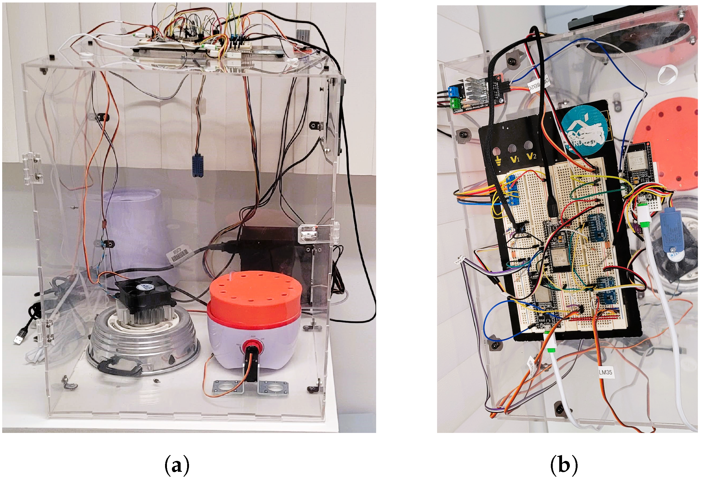
2. Air Heating and Humidification Experimental Module

The previously reported multivariable system [24,25] comprises an acrylic box with width, depth and height, in mm, given by 400, 400 and 500 respectively, equipped with an air heating and humidification system, as shown in Figure 1. Air heating is achieved through a 500 W resistance, and an ultrasonic mist generator is employed for air humidification. To monitor the temperature (controlled variable), a DS18B20 digital temperature sensor is installed inside the humidifier.

Figure 1a highlights the two main control study components installed in the module, an air heating resistance and the mist humidifier. Various sensors are installed to measure system variables of interest, with the Arduino board for data acquisition and system control highlighted in Figure 1b. Gas exhaust within the module is facilitated by a side-mounted fan. More details can be obtained elsewhere [24,25].

The process models are of the fractional order FOPDT type, and the control problem is a multivariable TITO servo type. This is shown below.

$$\left[\begin{array}{c}T\left(s\right)\\ H\left(s\right)\end{array}\right]=\left[\begin{array}{cc}{G}_{P11}\left(s\right)={\displaystyle \frac{K_{p11}·{\mathrm{e}}^{\left(-{\theta }_{p11}·s\right)}}{{\tau }_{p11}·s^{\left({\alpha }_{11}\right)}+1}}& G_{P12}\left(s\right)={\displaystyle \frac{K_{p12}·{\mathrm{e}}^{\left(-{\theta }_{p12}·s\right)}}{{\tau }_{p12}·s^{\left({\alpha }_{12}\right)}+1}}\\ G_{P21}\left(s\right)={\displaystyle \frac{K_{p21}·{\mathrm{e}}^{\left(-{\theta }_{p21}·s\right)}}{{\tau }_{p21}·s^{\left({\alpha }_{21}\right)}+1}}& G_{P22}\left(s\right)={\displaystyle \frac{K_{p22}·{\mathrm{e}}^{\left(-{\theta }_{p22}·s\right)}}{{\tau }_{p22}·s^{\left({\alpha }_{22}\right)}+1}}\end{array}\right]·\left[\begin{array}{c}V\left(s\right)\\ R\left(s\right)\end{array}\right]$$

(1)

In the matrix in (Equation (1)), the controlled variables are the following: $T\left(s\right)$ is the temperature, and $H\left(s\right)$ is the relative humidity of the air. The manipulated variables are the following: $R\left(s\right)$ is the resistance, and $V\left(s\right)$ is the voltage signal. The parameters ${\alpha }_{ij}$ are non-integers for models. The relationships defining the models are the following: $G_{P11}\left(s\right)$ relates temperature–voltage; $G_{P12}\left(s\right)$ relates temperature–resistance; $G_{P21}\left(s\right)$ relates humidity–voltage; $G_{P22}\left(s\right)$ relates humidity–resistance. In the control diagram, the variable $Y_1\left(s\right)$ corresponds to $T\left(s\right)$, $Y_2\left(s\right)$ corresponds to $H\left(s\right)$, $U_1\left(s\right)$ corresponds to $V\left(s\right)$, and $U_2\left(s\right)$ corresponds $R\left(s\right)$.

3. Tuning and Fractional Identification Based on PSO Metaheuristic Optimization

The procedures adopted for the studies on fractional identification and tuning of fractional controllers are based on the application of a particle swarm optimization (PSO) metaheuristic algorithm, as outlined in Appendix A, proposed by [27]. The PSO algorithm has proven to be suitable and highly effective in terms of convergence performance for the fractional modeling problems investigated in this work.

In a generic sense, we can consider the PSO algorithm as an optimizer where each particle is a potential solution in a $2D$ dimension. For example, each particle has a position $(x,y)$ and velocity $(v_x,v_y)$. The velocities of the particles determine their optimized movements for each particle generation, and for each particle, the update occurs based on two vectors: (a) the particle’s best position, $bestPos$; (b) the best position among all the particles, $bestGen$. Therefore, each particle aims to alter its position, given some basic information such as current positions, current velocities, the distance between the current position and $bestPos$, and the distance between the current position and $bestGen$. All movements in PSO then occur based on the following basic equations.

$$v_i^{\left(k+1\right)}=w·v_i^{\left(k\right)}+c_1·rand\left(\right)·\left(bestPo{s}_i-x_i^{\left(k\right)}\right)+c_2·rand\left(\right)·\left(bestGer-x_i^{\left(k\right)}\right)$$

(2)

$$x_i^{\left(k+1\right)}=x_i^{\left(k\right)}+v_i^{\left(k+1\right)}$$

(3)

where $v_i^{\left(k+1\right)}$ is the new velocity of the i-th particle; $v_i^{\left(k\right)}$ is the current velocity of the i-th particle; $c_1$ and $c_2$ are the cognitive and social learning parameters, respectively; w is the inertia weight parameter; $x_i^{\left(k\right)}$ is the current position of the i-th particle; $x_i^{\left(k+1\right)}$ is the new position of the i-th particle; $bestPo{s}_i$ is the best position of the i-th particle; $bestGer$ is the best position among all the particles; and $rand\left(\right)$ is the random value generator.

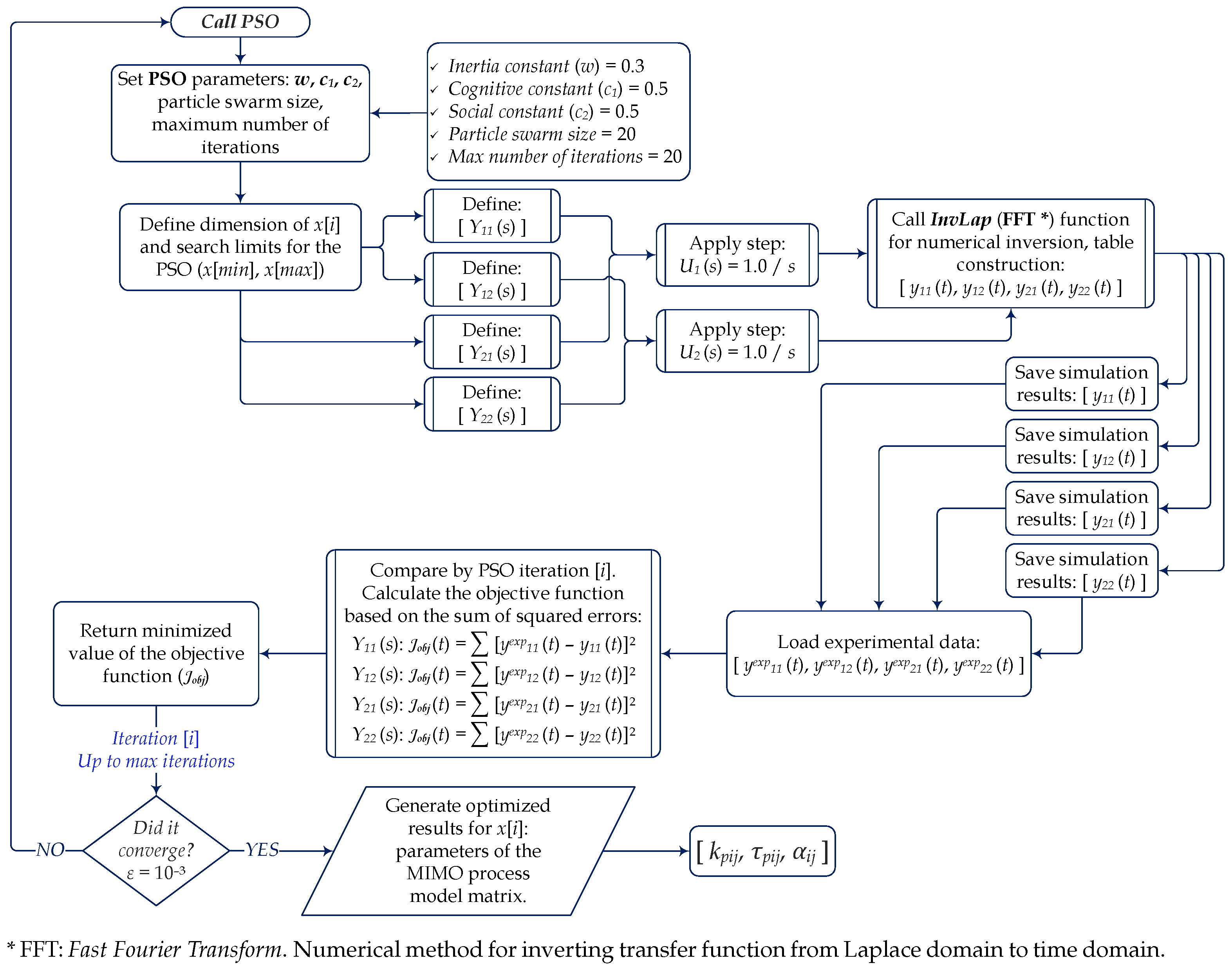
3.1. Open-Loop Identification Procedure

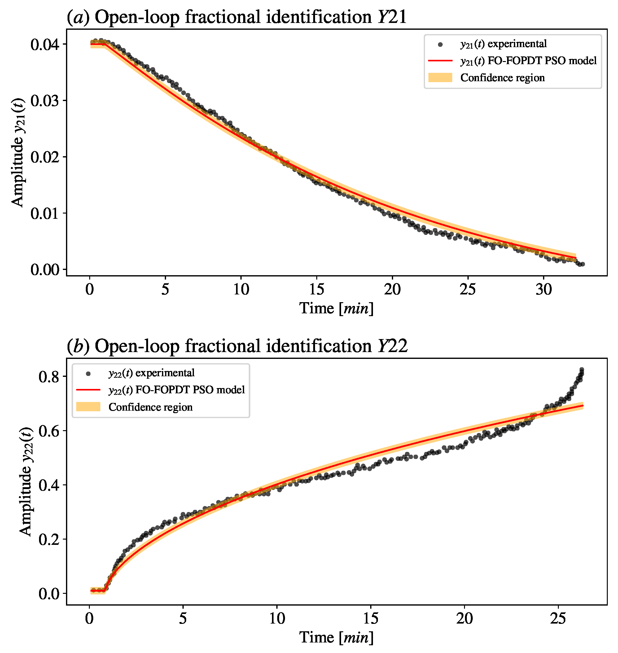
Open-loop identification was performed through parametric estimation using the PSO algorithm, which has proven to be effective in literature studies, notably for identifying multivariable systems. The overall concept of the open-loop identification procedure involves applying a unit positive step to the inputs $U_1\left(s\right)$ and $U_2\left(s\right)$ in the MIMO system corresponding to the experimental air heating and humidification module.

In Figure 2, a schematic diagram is presented with the methodological procedure for the open-loop identification of the MIMO system, the experimental air heating and humidification module, using the particle swarm optimization (PSO) metaheuristic method. Finally, it is worth mentioning that Appendix B presents further details regarding the algorithm used for the inversion of the Laplace Transform.

As depicted in Figure 2, the parameters to be optimized are the process gain ($k_p$), the process time constant (${\tau }_p$), and the fractional model parameter ($\alpha$):

$$x\left[i\right]={\left[k_{pij},{\tau }_{pij},{\alpha }_{ij}\right]}^{\mathrm{T}}$$

(4)

The execution of the adopted identification procedure follows the following cost function for optimization based on experimental data extracted from the work of [24] for constructing fractional-order models for each system model.

$$min{\mathcal{J}}_{obj}^{Y_{11}}\left(t\right)=\sum _{i=1}^{NE}{\left[y_{11\left(i\right)}^{EXP}\left(t\right)-y_{11\left(i\right)}^{PSO}\left(t\right)\right]}^2$$

(5)

$$min{\mathcal{J}}_{obj}^{Y_{12}}\left(t\right)=\sum _{i=1}^{NE}{\left[y_{12\left(i\right)}^{EXP}\left(t\right)-y_{12\left(i\right)}^{PSO}\left(t\right)\right]}^2$$

(6)

$$min{\mathcal{J}}_{obj}^{Y_{21}}\left(t\right)=\sum _{i=1}^{NE}{\left[y_{21\left(i\right)}^{EXP}\left(t\right)-y_{21\left(i\right)}^{PSO}\left(t\right)\right]}^2$$

(7)

$$min{\mathcal{J}}_{obj}^{Y_{22}}\left(t\right)=\sum _{i=1}^{NE}{\left[y_{22\left(i\right)}^{EXP}\left(t\right)-y_{22\left(i\right)}^{PSO}\left(t\right)\right]}^2$$

(8)

The superscript $EXP$ represents the experimental data from the module, and the superscript $PSO$ represents the simulated data from the model with parameter estimation determined by the application of the PSO algorithm. It is important to stress that the dead time (${\theta }_P$) was not re-estimated in the identification procedure since it is known from the open-loop identification conducted by [24,25] and it would not change significantly as it does not handle the fractional dynamics, differently from parameters K, $\tau$ and $\alpha$.

Therefore, considering the procedure for transfer functions $Y_{11}\left(s\right)$, $Y_{12}\left(s\right)$, $Y_{21}\left(s\right)$, and $Y_{22}\left(s\right)$ in Equations (5)–(8), it is necessary to adopt a single objective function to evaluate the best identification result globally. That is, the equation for ${\mathcal{F}}_{obj}^{Global}$ for this purpose takes the following form.

$$min{\mathcal{J}}_{obj}^{Global}\left(t\right)={\mathcal{J}}_{obj}^{Y_{11}}\left(t\right)+{\mathcal{J}}_{obj}^{Y_{12}}\left(t\right)+{\mathcal{J}}_{obj}^{Y_{21}}\left(t\right)+{\mathcal{J}}_{obj}^{Y_{22}}\left(t\right)$$

(9)

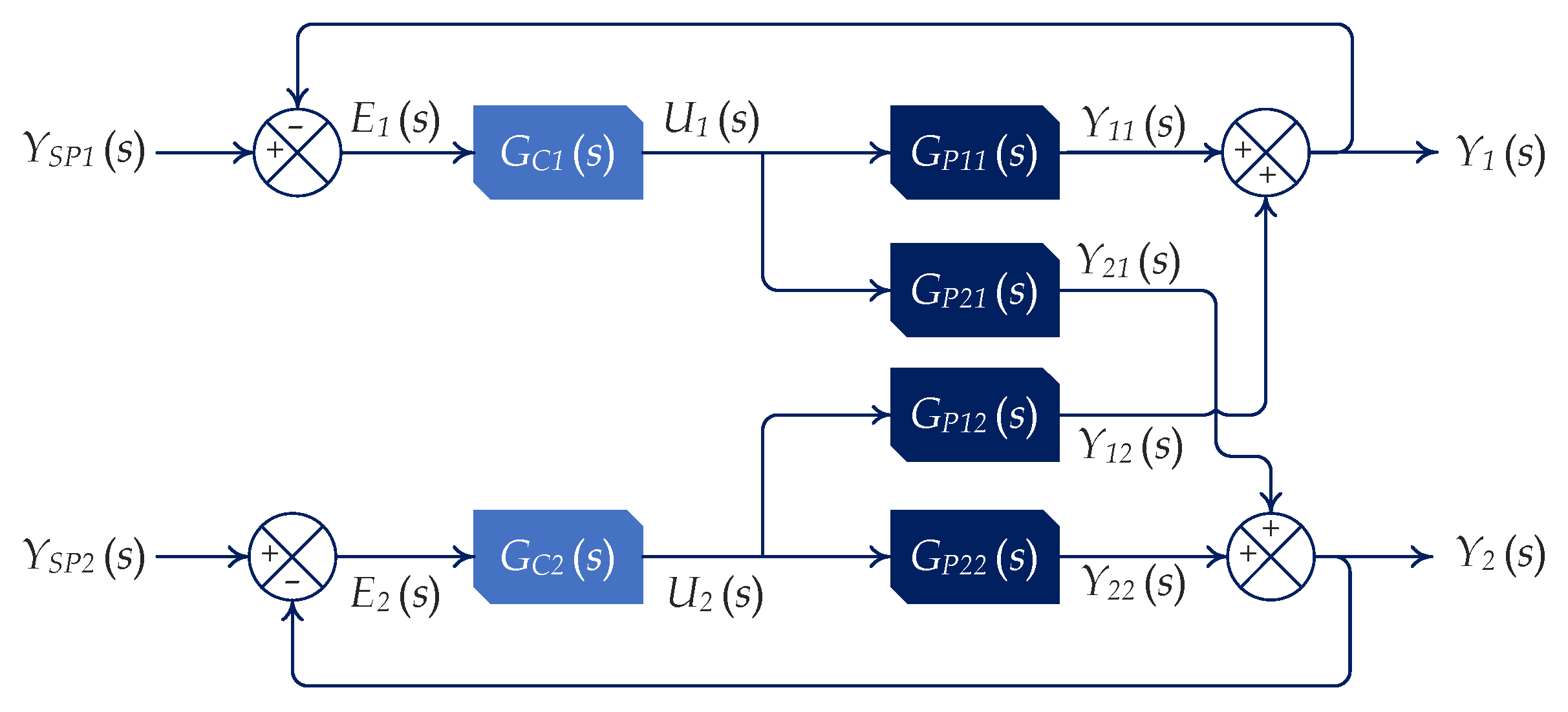
3.2. Design of the Fractional-Order Controller FOPI–PSO

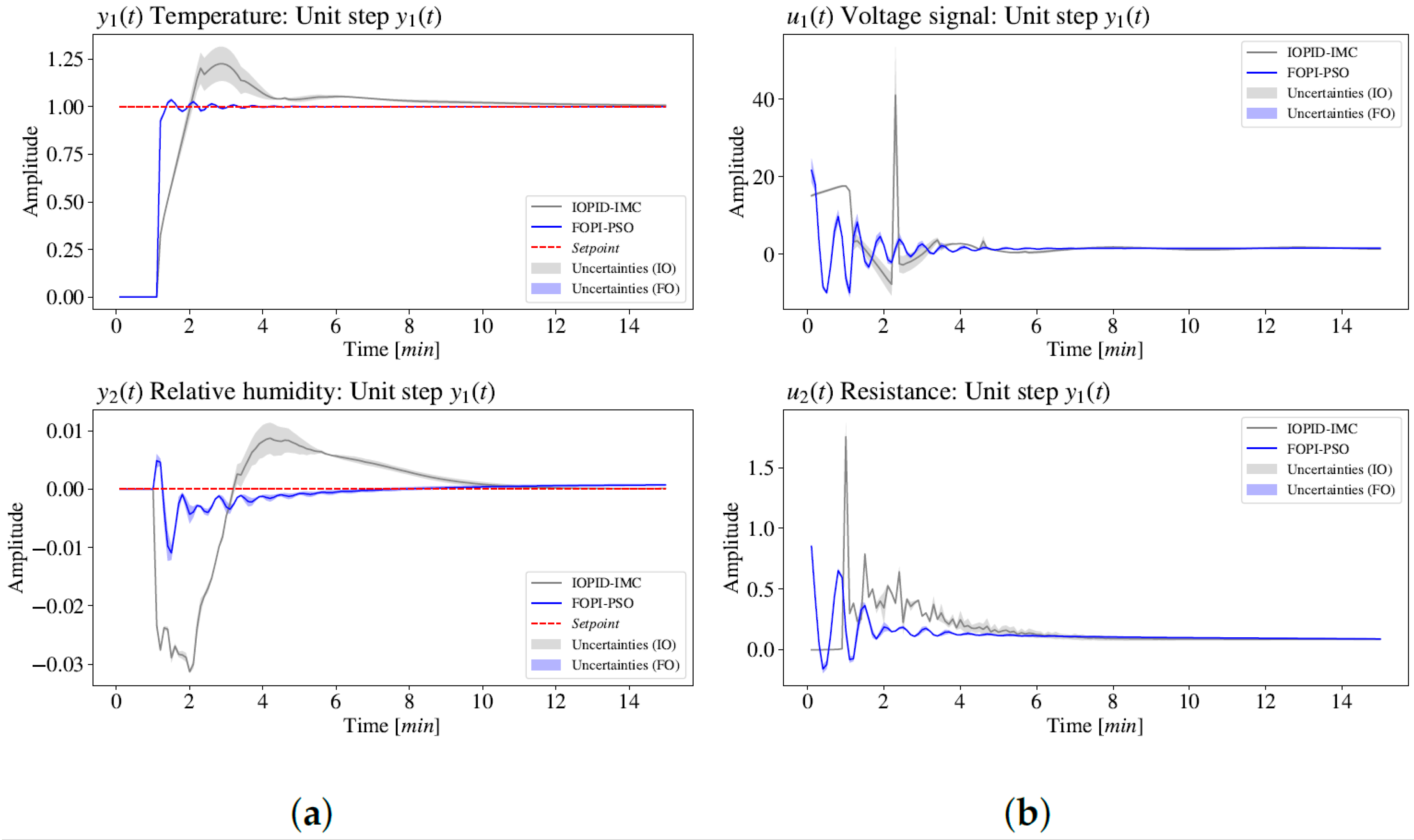
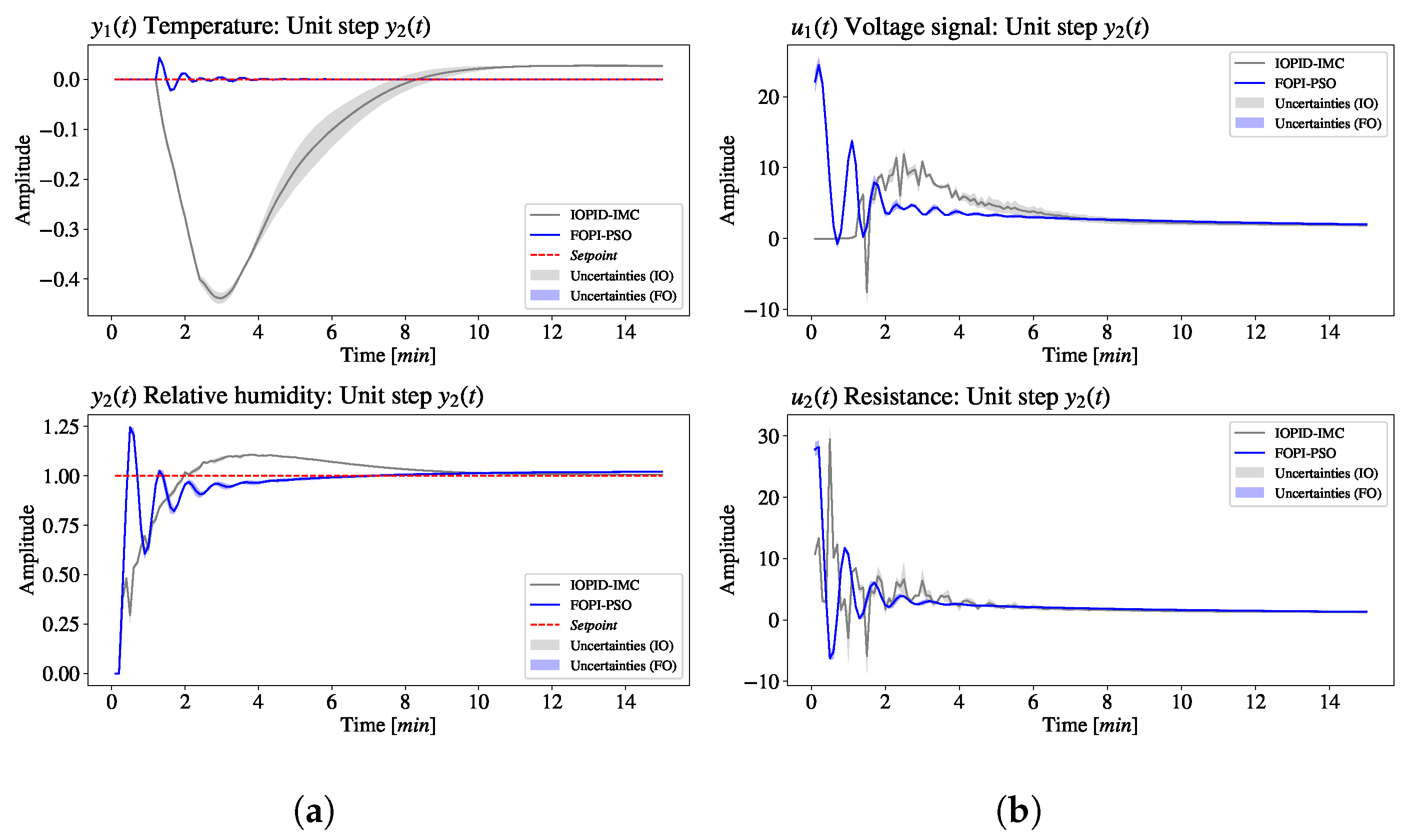
The MIMO system can be represented by a Two Input–Two Output (TITO) loop configuration because the module follows the structure of the diagram presented in Figure 3 without the use of loop decoupling. To conduct numerical simulation tests of the FO–MIMO loop, two unit step disturbances were applied to the setpoint. Initially, the disturbance was applied to $Y_1\left(s\right)$ ($Y_{SP1}=1/s$), while keeping $Y_2\left(s\right)$ constant in regulatory mode ($Y_{SP2}=0$). Subsequently, there was a switch to $Y_2\left(s\right)$ ($Y_{SP2}=1/s$), while keeping $Y_1\left(s\right)$ constant in regulatory mode ($Y_{SP1}=0$).

The selected controllers have an ideal FOPI structure (Equation (10)), with defined parametric uncertainties. Both structures were compared with their classical IOPID forms:

$$G_{Cj}\left(s\right)=\left(K_{Cj}\pm \sqrt{{\sigma }_{K_{Cj}}^2}\right)·\left[1+{\displaystyle \frac{1}{\left({\tau }_{Ij}\pm \sqrt{{\sigma }_{{\tau }_{Ij}}^2}\right)·s^{\left({\lambda }_j\pm \sqrt{{\sigma }_{{\lambda }_j}^2}\right)}}}\right],j=1,\cdots ,2$$

(10)

where $K_{Cj}$ is the proportionality constant and ${\tau }_{Ij}$ is the integrative time constant. The parameters ${\lambda }_j$ are fractional-order parameters for controllers. Parametric uncertainties are defined as $\pm \sqrt{{\sigma }^2}$ and determined through the stochastic Monte Carlo method.

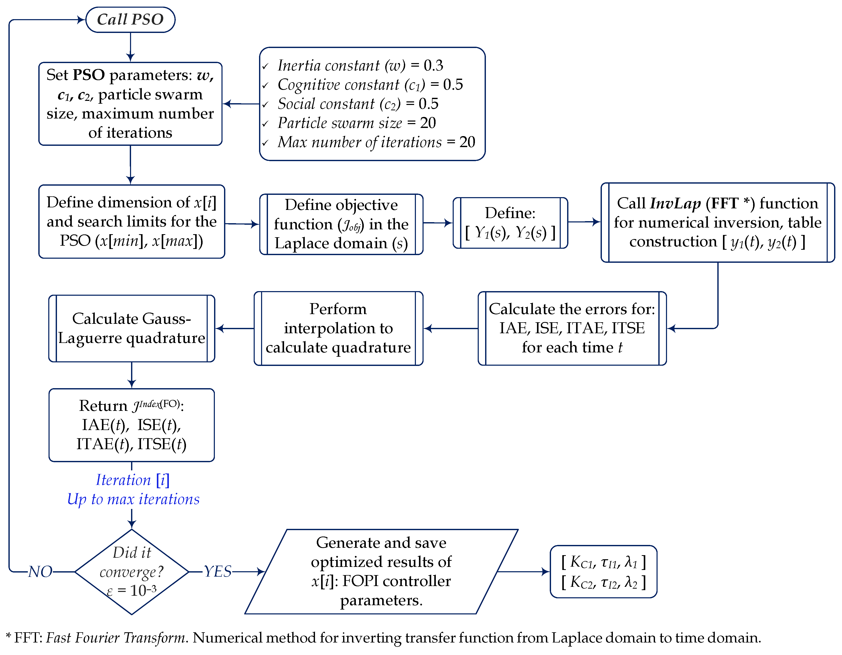
As it involves multivariable systems, the metaheuristic particle swarm optimization (PSO) method was adopted for investigations and tuning studies to parametrically estimate fractional-order proportional–integral (FOPI) controllers. However, it is necessary to define the objective function to be used to achieve the desired performance of the controllers. For the analysis of the studied multivariable control loops, the applied objective functions are integral-of-error-based indexes that demonstrated superior performance in the PSO tuning iterations. Their definitions are shown below.

• ISE (Integral Square Error):

  $$\mathrm{ISE}\left(t\right)={\int }_0^{\infty }{e}^2\left(t\right)dt={\int }_0^{\infty }{\left[y\left(t\right)-y_{SP}\left(t\right)\right]}^{2}dt$$

  (11)
• IAE (Integral Absolute value of Error):

  $$\mathrm{IAE}\left(t\right)={\int }_0^{\infty }\left|e\left(t\right)\right|dt={\int }_0^{\infty }\left|\left[y\left(t\right)-y_{SP}\left(t\right)\right]\right|dt$$

  (12)
• ITAE (Integral Time weighted Absolute Error):

  $$\mathrm{ITAE}\left(t\right)={\int }_0^{\infty }t\left|e\left(t\right)\right|dt={\int }_0^{\infty }t\left|\left[y\left(t\right)-y_{SP}\left(t\right)\right]\right|dt$$

  (13)
• ITSE (Integral Time weighted Square Error):

  $$\mathrm{ITSE}\left(t\right)={\int }_0^{\infty }t\left|e^2\left(t\right)\right|dt={\int }_0^{\infty }t\left|{\left[y\left(t\right)-y_{SP}\left(t\right)\right]}^2\right|dt$$

  (14)

In Equations (11)–(14), errors are defined as the difference between the dynamic responses of the controlled variables $y\left(t\right)$ and their desired setpoint reference $y_{SP}\left(t\right)$. However, a numerical procedure is necessary to solve the integrals of IAE, ISE, ITAE, and ITSE errors since analytical solutions are either unavailable or too complex, demanding substantial computational effort. One way to overcome this issue is through the numerical estimation of the integral using the Gauss quadrature technique, where Gauss–Legendre quadrature was adopted.

A critical issue in this work is the evaluation of the tuning quality and performance of the control loops. Toward this, the analysis is based on the minimization indexes of errors defined in Equations (11)–(14), widely applied in process control engineering. Another way to assist in the performance analysis of control loops is the determination of the integral of manipulated variables $IU\left(t\right)$ with N manipulated variables, also known as effort or control energy of MIMO loops.

$$\mathrm{IU}\left(t\right)={\int }_0^{\infty }\left|U_j\left(t\right)\right|dt,j=1,\dots ,N$$

(15)

However, since we are dealing with multivariable systems with a multi-loop structure and variable pairing, it is more interesting to apply the sum of the performance indexes. The goal is to maintain both controlled variables stable within the specified reference setpoint, with reduced and smoothed action on manipulated variables. The equations for the objective functions to assess the performance of the studied control structures in simulations for the servo problem are presented below, based on the minimization of the ISE, IAE, ITAE, ITSE, and IU indexes for the controlled variables $y_j$ and manipulated variables $u_j$ in TITO systems (loops $L1$ and $L2$) [28].

$$min{\mathcal{J}}^{IAE}\left(t\right)={\left[{\mathrm{IAE}}_{L1}^{\left(y_1\right)}\left(t\right)+{\mathrm{IAE}}_{L2}^{\left(y_2\right)}\left(t\right)\right]}_{step{y}_1}+{\left[{\mathrm{IAE}}_{L1}^{\left(y_1\right)}\left(t\right)+{\mathrm{IAE}}_{L2}^{\left(y_2\right)}\left(t\right)\right]}_{step{y}_2}$$

(16)

$$min{\mathcal{J}}^{ISE}\left(t\right)={\left[{\mathrm{ISE}}_{L1}^{\left(y_1\right)}\left(t\right)+{\mathrm{ISE}}_{L2}^{\left(y_2\right)}\left(t\right)\right]}_{step{y}_1}+{\left[{\mathrm{ISE}}_{L1}^{\left(y_1\right)}\left(t\right)+{\mathrm{ISE}}_{L2}^{\left(y_2\right)}\left(t\right)\right]}_{step{y}_2}$$

(17)

$$min{\mathcal{J}}^{ITAE}\left(t\right)={\left[{\mathrm{ITAE}}_{L1}^{\left(y_1\right)}\left(t\right)+{\mathrm{ITAE}}_{L2}^{\left(y_2\right)}\left(t\right)\right]}_{step{y}_1}+{\left[{\mathrm{ITAE}}_{L1}^{\left(y_1\right)}\left(t\right)+{\mathrm{ITAE}}_{L2}^{\left(y_2\right)}\left(t\right)\right]}_{step{y}_2}$$

(18)

$$min{\mathcal{J}}^{ITSE}\left(t\right)={\left[{\mathrm{ITSE}}_{L1}^{\left(y_1\right)}\left(t\right)+{\mathrm{ITSE}}_{L2}^{\left(y_2\right)}\left(t\right)\right]}_{step{y}_1}+{\left[{\mathrm{ITSE}}_{L1}^{\left(y_1\right)}\left(t\right)+{\mathrm{ITSE}}_{L2}^{\left(y_2\right)}\left(t\right)\right]}_{step{y}_2}$$

(19)

$$min{\mathcal{J}}^{IU}\left(t\right)={\left[{\mathrm{IU}}_{L1}^{\left(u_1\right)}\left(t\right)+{\mathrm{IU}}_{L2}^{\left(u_2\right)}\left(t\right)\right]}_{step{y}_1}+{\left[{\mathrm{IU}}_{L1}^{\left(u_1\right)}\left(t\right)+{\mathrm{IU}}_{L2}^{\left(u_2\right)}\left(t\right)\right]}_{step{y}_2}$$

(20)

Equations (16)–(19) represent the objective function ($\mathcal{J}\left(t\right)$ ) for tuning control loops, characterized by the performance indexes of errors: $\mathrm{IAE}\left(t\right)$, $\mathrm{ISE}\left(t\right)$, $\mathrm{ITAE}\left(t\right)$ and $\mathrm{ITSE}\left(t\right)$. With the defined objective functions, a particle swarm optimization (PSO) algorithm is then applied to determine the optimal parameters of the FOPI controllers. A flowchart outlining the procedure is presented in Figure 4 for tuning the parameters of the studied controllers using the standard particle swarm optimization (PSO) algorithm.

The parameters of the PSO algorithm were selected based on computational effort and the convergence of the error defined as $\epsilon ={10}^{-3}$. In this context, the particle size and maximum number of iterations proved to be sufficient for the convergence of the optimization procedure.

Therefore, we can globally sum the performance indexes as a criterion for easier selection of the best-tuned parameters analyzed as follows.

$$min{\mathcal{J}}^{Global}\left(t\right)={\mathcal{J}}^{IAE}\left(t\right)+{\mathcal{J}}^{ISE}\left(t\right)+{\mathcal{J}}^{ITAE}\left(t\right)+{\mathcal{J}}^{ITSE}\left(t\right)+{\mathcal{J}}^{IU}\left(t\right)$$

(21)

Another way to analyze the performance of the dynamic responses of the studied control systems is through the calculation of the percentage of relative gain (${\mathcal{P}}_{\%}^{Index}$) in terms of the reduction of the performance indexes previously defined as objective functions for parameter tuning and the evaluation of the quality of these tunings. This is always in reference to the integer-order control structures (IOPID) found in the literature. These gains can be defined as follows.

$${\mathcal{P}}_{\%}^{Index}=\left({\displaystyle \frac{{\mathcal{J}}^{Index\left(\mathrm{IO}\right)}-{\mathcal{J}}^{Index\left(\mathrm{FO}\right)}}{{\mathcal{J}}^{Index\left(\mathrm{IO}\right)}}}\right)$$

(22)

$${\mathcal{P}}_{\%}^{Global}=\left({\displaystyle \frac{{\mathcal{J}}^{Global\left(\mathrm{IO}\right)}-{\mathcal{J}}^{Global\left(\mathrm{FO}\right)}}{{\mathcal{J}}^{Global\left(\mathrm{IO}\right)}}}\right)$$

(23)

where the ($Index$) is equivalent to the ISE, IAE, ITAE, and ITSE, Equations (11)–(14). The indices (IO) and (FO) denote the strategies of integer-order and fractional-order control, respectively, applied for the determination of the indexes.

4. Results

4.1. Fractional Open-Loop Identification

Based on the experimental data extracted from the literature [24,25], simulations were carried out using the PSO optimization algorithm for the open-loop identification of the fractional-order model matrix (FO-FOPDT) of the MIMO system corresponding to the experimental air heating and humidification module. The parametric estimation obtained after five experimental attempts of PSO algorithm cycles is presented in

Table 1. Open-loop fractional identification results for the process model matrix.

Parameters	IO–FOPDT Nelder–Mead	FO–FOPDT PSO
$k_{pij}$	$\left[\begin{array}{cc}0.762\pm 0.001& -1.115\pm 0.009\\ -0.044\pm 5.000·{10}^{-4}& 0.670\pm 0.030\end{array}\right]$	$\left[\begin{array}{cc}0.643\pm 6.258·{10}^{-3}& -0.895\pm 9.025·{10}^{-3}\\ -0.047\pm 4.847·{10}^{-4}& 2.700\pm 2.706·{10}^{-2}\end{array}\right]$
${\tau }_{pij}$ [min]	$\left[\begin{array}{cc}18.223\pm 0.120& 13.303\pm 0.162\\ 12.385\pm 0.201& 2.491\pm 0.365\end{array}\right]$	$\left[\begin{array}{cc}16.922\pm 0.171& 19.893\pm 0.198\\ 22.472\pm 0.217& 27.882\pm 0.283\end{array}\right]$
${\alpha }_{ij}$	–	$\left[\begin{array}{cc}1.108\pm 1.128·{10}^{-2}& 1.146\pm 1.220·{10}^{-2}\\ 1.046\pm 1.126·{10}^{-2}& 0.633\pm 6.208·{10}^{-3}\end{array}\right]$
$R_{ij}$	$$\left[\begin{array}{cc}0.998& 0.996\\ 0.990& 0.968\end{array}\right]$$	$$\left[\begin{array}{cc}1.000& 0.996\\ 0.999& 0.985\end{array}\right]$$
${\mathcal{J}}_{obj}^{Global}$	1.779	1.364

IO–FOPDT Nelder–Mead: first-order models with integer-order dead time with parameter estimation using the Nelder–Mead method according to [24]; FO–FOPDT PSO: First-order plus fractional dead time models with PSO parametric estimation. $R_{ij}$: matrix of Pearson correlation coefficients; ${\mathcal{J}}_{obj}^{global}$: global objective function from Equation (9).

, where the parameters are compared with integer-order models and the deterministic Nelder–Mead method. The parametric uncertainties of the estimated parameters for the fractional-order models were determined using the stochastic Monte Carlo algorithm, while the system delay times were not re-estimated, considering the values as defined by [24].

The identification results are illustrated in Figure 5 for the responses of $Y_{11}\left(s\right)$ and $Y_{12}\left(s\right)$ to a unit step in $U_1\left(s\right)$. Figure 6, in turn, presents the responses of $Y_{21}\left(s\right)$ and $Y_{22}\left(s\right)$ to a unit step in $U_2\left(s\right)$. The simulated behaviors of the models relating the temperature and relative humidity of the air exhibit amplitude responses in deviation variables.

4.2. Fractional Control Experimental Module

As a reference for comparison, the integer-order IOPID-IMC controller proposed by Daga [24,25] was adopted, with the ideal structure as given by Equation (24) below.

$$G_{Cj}\left(s\right)=\left(K_{Cj}\pm \sqrt{{\sigma }_{K_{Cj}}^2}\right)·\left(1+{\displaystyle \frac{1}{\left({\tau }_{Ij}\pm \sqrt{{\sigma }_{{\tau }_{Ij}}^2}\right)·s}}+\left({\tau }_{Dj}\pm \sqrt{{\sigma }_{{\tau }_{Dj}}^2}\right)·s\right)$$

(24)

Therefore, the vector of IOPID–IMC controllers has the following form.

$$G_C^{\left(\mathrm{IO}\right)}\left(s\right)=\left[\begin{array}{c}{G}_{C1}\left(s\right)=\left(18.970\pm 1.834\right)·\left(1+{\displaystyle \frac{1}{\left(9.687\pm 0.953\right)·s}}+\left(0.557\pm 0.055\right)·s\right)\\ G_{C2}\left(s\right)=\left(9.760\pm 1.007\right)·\left(1+{\displaystyle \frac{1}{\left(1.370\pm 0.142\right)·s}}+\left(0.119\pm 0.012\right)·s\right)\end{array}\right]$$

(25)

Regarding the reduction of errors associated with the control loops, it can be observed that the FOPI–PSO controller, with the objective function based on ITAE, namely ${\mathcal{J}}^{ITAE}$, demonstrated superior performance in percentage terms, as shown in

Table 2. FOPI–PSO and IOPID–IMC comparison for the heating and humidification experimental module.

Controller ‡	${\mathcal{J}}^{\mathit{IAE}}$	${\mathcal{J}}^{\mathit{ISE}}$	${\mathcal{J}}^{\mathit{ITAE}}$	${\mathcal{J}}^{\mathit{ITSE}}$	${\mathcal{J}}^{\mathit{IU}}$	${\mathcal{J}}^{\mathit{Global}}$
IOPID–IMC [24]	4.734	2.079	14.876	2.844	127.071	151.6
FOPI–PSO	1.845	1.302	3.034	0.794	111.778	118.8
Gain	${\mathcal{P}}_{\%}^{IAE}$	${\mathcal{P}}_{\%}^{ISE}$	${\mathcal{P}}_{\%}^{ITAE}$	${\mathcal{P}}_{\%}^{ITSE}$	${\mathcal{P}}_{\%}^{IU}$	${\mathcal{P}}_{\%}^{Global}$
FOPI–PSO	61.0%	37.4%	79.6%	72.1%	12.0%	22%

^‡ IOPID–IMC: PID integer-order controller tuned by the IMC method; FOPI–PSO: PI fractional-order controller with tuning via PSO optimization.

, achieving a global gain of 22% compared to IOPID–IMC. It is important to emphasize that the structures of the compared controllers have the same number of parameters; however, the FOPI controller is non-integer order, with parameters ${\lambda }_j$ (PI^λ) characterized by the incorporation of memory effect in control actions.

The modeling of the system is known and determined through open-loop identification studies, obtaining fractional models for the TITO system. With the FOPI–PSO controller parameters and the fractional FO–FOPDT models of the process defined, closed-loop simulation studies were conducted, including the propagation of uncertainties determined by the Monte Carlo method. In this context, the matrix with FO–FOPFT models (Equation (26)) and the FOPI-PSO control vector (Equation (27)) are defined as follows.

$$G_P\left(s\right)=\left[\begin{array}{cc}{G}_{P11}\left(s\right)={\displaystyle \frac{\left(0.643\right)·{\mathrm{e}}^{\left(-1.15·s\right)}}{\left(16.922\right)·s^{\left(1.108\right)}+1}}& G_{P12}\left(s\right)={\displaystyle \frac{\left(-0.895\right)·{\mathrm{e}}^{\left(-1.25·s\right)}}{\left(19.893\right)·s^{\left(1.146\right)}+1}}\\ G_{P21}\left(s\right)={\displaystyle \frac{\left(-0.047\right)·{\mathrm{e}}^{\left(-s\right)}}{\left(22.472\right)·s^{\left(1.046\right)}+1}}& G_{P22}\left(s\right)={\displaystyle \frac{\left(2.700\right)·{\mathrm{e}}^{\left(-0.25·s\right)}}{\left(27.882\right)·s^{\left(0.633\right)}+1}}\end{array}\right]$$

(26)

$$G_C^{\left(\mathrm{FO}\right)}\left(s\right)=\left[\begin{array}{c}{G}_{C1}\left(s\right)=\left(37.331\pm 3.788·{10}^{-1}\right)·\left[1+{\displaystyle \frac{1}{\left(0.060\pm 6.049·{10}^{-4}\right)·s^{\left(0.681\pm 6.589·{10}^{-3}\right)}}}\right]\\ G_{C2}\left(s\right)=\left(27.872\pm 1.435·{10}^{-1}\right)·\left[1+{\displaystyle \frac{1}{\left(12.061\pm 1.435·{10}^{-2}\right)·s^{\left(1.144\pm 4.341·{10}^{-5}\right)}}}\right]\end{array}\right]$$

(27)

In Equation (26), the time delay (${\theta }_{Pj}$) of the process models has disregarded uncertainties due to the characteristics of open-loop identification for the experimental module.

In Table 2, for the Global performance metrics, the definition consists of the simple sum of the indeces, aiming to facilitate the comparison between control proposals, as follows.

$${\mathcal{J}}_{obj}^{Global}=\sum _{i=1}^{N=2}{\mathcal{J}}_{obj}^{IAE}+\sum _{i=1}^{N=2}{\mathcal{J}}_{obj}^{ISE}+\sum _{i=1}^{N=2}{\mathcal{J}}_{obj}^{ITAE}+\sum _{i=1}^{N=2}{\mathcal{J}}_{obj}^{ITSE}+\sum _{i=1}^{N=2}{\mathcal{J}}_{obj}^{IU}$$

(28)

In Equation (28), $i=1,\cdots ,N$ represents loop 1 ($Y_1$—air temperature) and loop 2 ($Y_2$—air humidity). In this context, the overall relative gain of FOPI control compared to IOPID for a unit step in air temperature ($Y_1$) is 42.7%, while the overall relative gain for a unit step in air humidity ($Y_2$) reached 12.1%. It is important to highlight that significant performance improvements were achieved when analyzing the control loops separately, with index reduction gains in the range of 40–100%. Regarding the robustness of fractional control, it is worth noting the significant reduction in the ${\mathcal{P}}_{\%}^{IU}$ index, with gains of around 40% for loop 1, controlling air temperature with a step in $Y_{SP1}\left(s\right)$.

When conducting simulation studies for the TITO loop of the experimental air heating and humidification module, Figure 7 illustrates the dynamics of the controlled and manipulated variables during a step input applied to $Y_1\left(s\right)$ (air temperature), while keeping $Y_2\left(s\right)$ constant (air humidity). The responses are presented in terms of amplitude. Subsequently, in Figure 8, the simulation results are shown with the reversal of the step input application, i.e., applying the step to $Y_2\left(s\right)$ (relative air humidity) while keeping $Y_1\left(s\right)$ constant (air temperature), also with responses in amplitude.

A dynamic temporal parameter analysis was also performed, as shown in

Table 3. Dynamic temporal parameters for FOPI–PSO and IOPID–IMC controllers with a unit step input at the setpoint $y_1\left(t\right)$ (temperature).

Controller ‡	Rise Time [min]	Settling Time [min]	Overshoot $[\%]$	Undershoot $[\%]$	Peak	Peak Time [min]
IOPID-IMC: $Y_1\left(s\right)$	1.20	6.10	21.68	1.97	1.23	2.90
FOPI-PSO: $Y_1\left(s\right)$	1.20	1.60	3.62	1.72	1.04	1.50
IOPID-IMC: $Y_2\left(s\right)$	3.20	4.60	0.86	3.14	0.01	4.20
FOPI-PSO: $Y_2\left(s\right)$	1.10	6.80	0.41	1.16	0.005	1.10

^‡ IOPID–IMC: PID integer-order controller tuned by the IMC method [24]; FOPI–PSO: PI fractional-order controller with tuning via PSO optimization.

, considering the responses of the controlled variables with the setpoint at $Y_1\left(s\right)$, and in

Table 4. Dynamic temporal parameters for FOPI–PSO and IOPID–IMC controllers with a unit step input at the setpoint $y_2\left(t\right)$ (relative humidity).

Controller ‡	Rise Time [min]	Settling Time [min]	Overshoot $[\%]$	Undershoot $[\%]$	Peak	Peak Time [min]
IOPID-IMC: $Y_1\left(s\right)$	8.50	13.10	0.02	45.34	0.03	13.10
FOPI-PSO: $Y_1\left(s\right)$	1.30	7.10	4.37	2.15	0.04	1.30
IOPID-IMC: $Y_2\left(s\right)$	1.40	4.30	10.06	1.20	1.11	3.80
FOPI-PSO: $Y_2\left(s\right)$	0.30	3.70	22.13	0.55	1.25	0.50

^‡ IOPID–IMC: PID integer-order controller tuned by the IMC method [24]; FOPI–PSO: PI fractional-order controller with tuning via PSO optimization.

, with the setpoint switched to $Y_2\left(s\right)$. These tables present the response quality metrics of the control loops studied, specifically including Rise Time, Settling Time, Overshoot, Undershoot, Peak, and Peak Time for both the IOPID–IMC and FOPI–PSO controllers.

5. Discussion

From the analysis of results, the choice of the FOPI–PSO controller based on ITAE is justified by the weighting between the reduction in IAE, ISE, ITAE, and ITSE criteria and the criterion based on the movement of manipulated variables, i.e., the IU index of the integral of $U_1\left(s\right)$ and $U_2\left(s\right)$. The 12% reduction in the IU index indicates lower energy consumption (or control effort) for the desired control action. The performance of the FOPI-PSO control proposal was validated through simulation studies, applying a unit step in $Y_{SP1}\left(s\right)$ and alternating the simulation with a step in $Y_{SP2}\left(s\right)$ in a servo-type control structure. This same procedure was also adopted for the tunings with the PSO optimization algorithm.

All results for the TITO experimental system demonstrate the high performance and robustness of the FOPI–PSO control proposal compared to the reference, which uses the implementation of the IOPID–IMC controller implemented by [24]. This behavior can be observed in Table 2 for the unit step in $Y_{SP1}$ and $Y_{SP2}$, with the determination of IAE, ISE, ITAE, ITSE, and IU criteria, highlighting the percentage relative gain of FOPI–PSO controllers. In this context, the overall relative gain (${\mathcal{P}}_{\%}^{Global}$) of FOPI control compared to IOPID–IMC is 22%, reaching up to 79.6% gain in ITAE and 72.1% for ITSE reduction. Therefore, the proposed FOPI–PSO controller significantly improved the performance and robustness of the control system, leading to promising gains of the fractional strategy applied to the experimental air heating and humidification system.

Simulations of the control loops also demonstrate the high speed of responses to the tracking setpoint. This highlights the superiority of fractional strategies compared to classical IOPID approaches.

6. Conclusions

This paper explored an experimental MIMO system of an air heating and humidification module using experimental data extracted from [24,25]. For this purpose, fractional-order identification studies were carried out in the open-loop models of the process (FO–FOPDT). Superior results were observed with FO–FOPDT-type models, as evidenced by the models’ behaviors depicted in comparison with experimental data.

With the identified fractional process models, tuning and closed-loop system simulation were conducted to validate the proposal, using a fractional-order FOPI–PSO control structure. In other words, fractional control was implemented with controller parameter estimation through the PSO metaheuristic algorithm. Tests were conducted using objective functions based on the integrals of IAE, ISE, ITAE, and ITSE errors, with the most favorable results obtained with $min{\mathcal{J}}_{obj}=ITAE$.

The closed-loop simulations, using the FO–FOPDT-type model matrix and fractional controllers $G_{C1}^{\left(\mathrm{FO}\right)}\left(s\right)$ and $G_{C2}^{\left(\mathrm{FO}\right)}\left(s\right)$ of the PI^λ fractional type (FOPI–PSO), were compared with the strategy proposed by [24,25], which employed IOPID–IMC controllers and confirmed the high performance and robustness of the developed FOPI fractional approach in the works, showing a global gain of 22%. The robustness of the fractional proposal is also evidenced when evaluating the quality metric reduction gains for manipulated variables, which obtained gains of 12%, as denoted by the ${\mathcal{P}}_{\%}^{IU}$ index.

The FOPI–PSO control proposal with the objective function for the PSO algorithm based on IAE yielded a global gain of 42.7% reduction when analyzing the performance with a step in $Y_{SP1}\left(s\right)$. Particularly for this case study, gains were also highlighted in the control effort of the manipulated variables defined by the IU index, with a reduction of approximately 39.8% with fractional control. For this experimental module, the application of fractional calculus in the design of the MIMO system significantly enhanced the performance and robustness of the developed control system.

In summary, this work contributes to a better understanding and validation of fractional calculus applications for the design of FO–MIMO systems, with promising and superior performance in terms of gains from the developed fractional FOPI controllers compared to classical strategies of integer-order IOPID. Additionally, the experimental module system was explored with fractional order process models, contributing to increasing the robustness of the implemented control systems.