Control Error Convergence Using Lyapunov Direct Method Approach for Mixed Fractional Order Model Reference Adaptive Control

Abstract

This paper extends Lyapunov stability theory to mixed fractional order direct model reference adaptive control (FO-DMRAC), where the adaptive control parameter is of fractional order, and the control error model is of integer order. The proposed approach can also be applied to other types of model reference adaptive controllers (MRACs), provided the form of the control error dynamics and the fractional order adaptive control law are similar. This paper demonstrates that the control error will converge to zero, even if the derivative of the classical Lyapunov function $\dot{V}$ is positive during a transient period, as long as $\dot{V}(e,\varphi )$ tends to zero as time approaches infinity. Finally, this paper provides application examples that illustrate both the convergence of the control error to zero and the behavior of $\dot{V}(e,\varphi )$.

1. Introduction

This paper extends the classical Lyapunov stability theory to mixed fractional order direct model reference adaptive control (FO-DMRAC), providing a theoretical foundation for analyzing the stability of fractional order dynamic systems. The principal aim of this paper is to demonstrate that, for such systems, the control error $e_1\left(t\right)$ approaches zero as time tends to infinity, leveraging the classical Lyapunov stability approach.

This work prioritizes establishing that the control error $e_1\left(t\right)=y_p\left(t\right)-y_m\left(t\right)$ converges to zero, even if the Lyapunov method ($\dot{V}(e,\varphi )\le 0$) conditions are not met for all $t$ The analysis shows that this convergence holds as long as the difference between the plant output $y_p\left(t\right)$ and the reference model output $y_m\left(t\right)$ approaches zero as $t\to \infty$.

Numerous methods applied to fractional adaptive systems rely on fractional Lyapunov functions [1,2], resulting in analyses that primarily ensure the stability of the mean square of the control error [3,4,5,6,7]. For instance, the approach presented in [4] develops a specialized fractional Lyapunov function tailored for fractional order dynamic systems. Similarly, the works of [5] and [6] propose the use of fractional Lyapunov derivatives to address an adaptive class of fractional systems, but those methods do not use the classical or integer Lyapunov approach. Additionally, other noteworthy approaches include the utilization of fractional gradients for control applications [8,9,10,11,12,13,14,15] and adaptive laws based on the MIT rule [8,9,10]. However, these approaches often lack rigorous stability analysis, and the proposed fractional Lyapunov functions tend to be quite complex.

For this reason, this work seeks to perform a stability analysis using a classical Lyapunov function but applied to a fractional controller, thus decreasing the analysis’s complexity level. To conduct this analysis, we utilized the adaptive error model 3, which operates without access to the system’s states. This approach adds complexity and generality to the analysis while simultaneously ensuring that the control error converges to zero [1,2]. It is worth mentioning that fractional calculus could be used in the case of Lyapunov exponent problems if we change the classical derivative to a fractional one [16].

This paper is structured as follows: Section 2 presents the classical integer order implementation of direct model reference adaptive control (IO-DMRAC). In Section 3, we explore fundamental concepts and key results from fractional calculus, which serve as the foundation for analyzing the stability of FO-DMRAC systems. Section 4 addresses the challenges associated with proving the convergence of the control error $e_1\left(t\right)$ to zero and introduces the proposed methodology for establishing this convergence. Section 5 showcases the simulation results across various examples that illustrate both the convergence of the control error to zero and the behavior of the function $\dot{V}(e,\varphi )$ Lastly, Section 6 summarizes the conclusions.

2. Control Model System

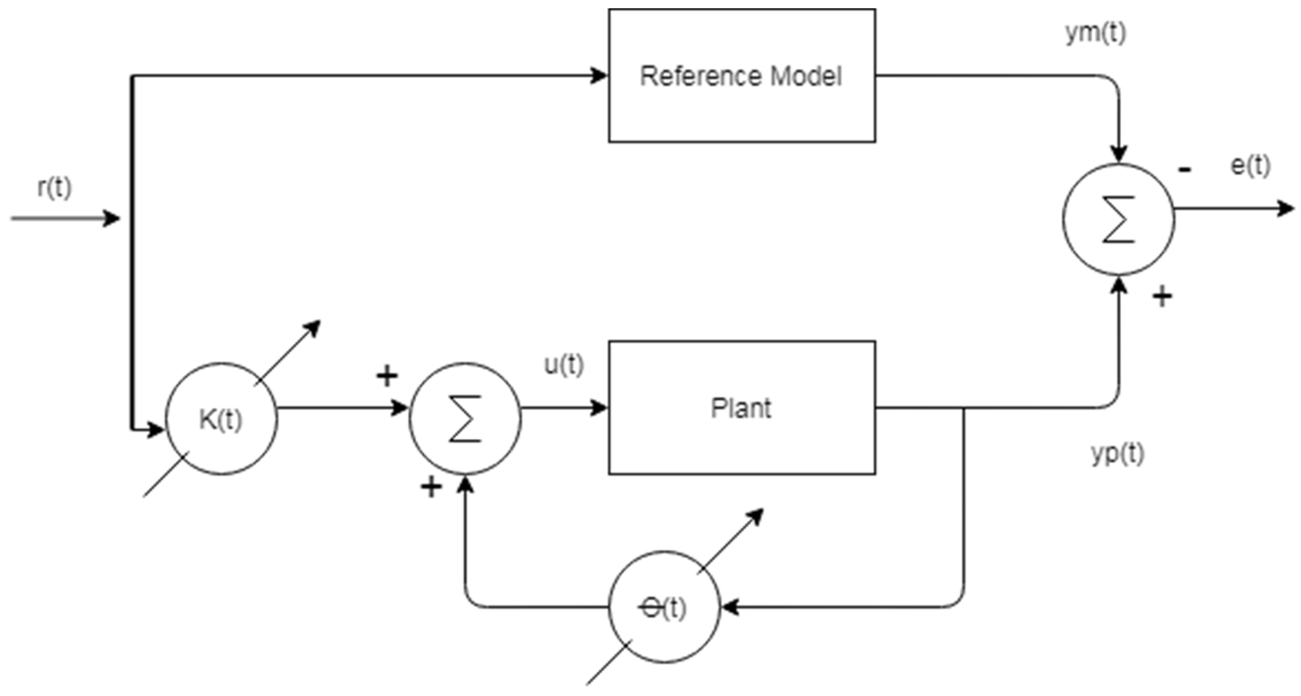
Figure 1 shows a simplified block diagram for the classical integer order direct model reference adaptive control (DMRAC), in which control parameters $k$ and $\theta$ are adjusted using their corresponding adaptive laws to keep the control error as small as possible.

DMRAC Algorithm

The objective of the DMRAC is to minimize the control error $e_1\left(t\right)$ This approach simplifies implementation by eliminating the need for an identification block, as asymptotic convergence of the controller parameters to their ideal values is not required, making parameter adjustments less critical [17].

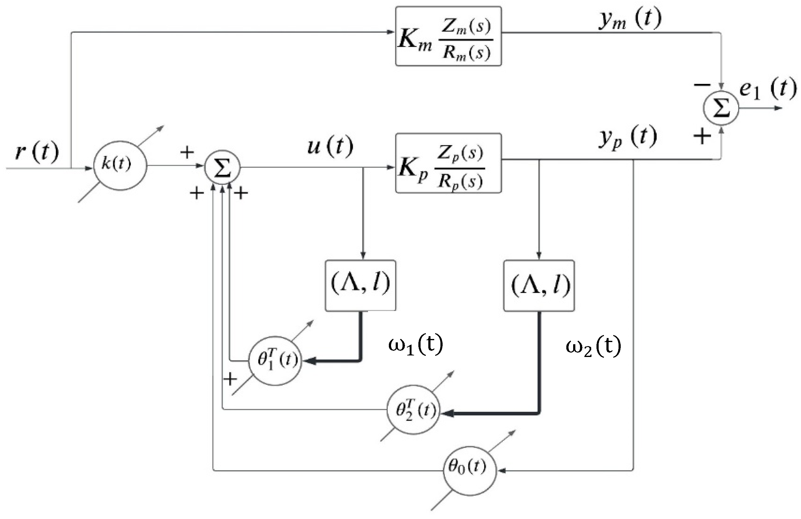
In Figure 2, a detail DMRAC adaptive control scheme of a linear (or linearized) nth order plant, with relative degree 1 $\left(n^{*}=1\right)$, is shown. In this scheme, only the control error $e_1\left(t\right)$ is accessible (error model 3), while the full state error vector $e\left(t\right)$ is not. This limitation simplifies the analysis of the stability conditions [17]. Next, we show the differences between error models 2 and 3, respectively.

Model error 2:

${}_{t_0}{}^{C}D_t^{\beta }e\left(t\right)=A_{mn}e\left(t\right)+b_{mn}\left[{\varphi }^T\left(t\right)\omega \left(t\right)\right],e\left(t_0\right)=e_0$. In this case, the whole sate error vector $e\left(t\right)$ is accessible, including the output or control error $e_1\left(t\right)$, which is one element of the state vector.

Model error 3:

$${}_{t_0}{}^{C}D_t^{\beta }e\left(t\right)=A_{mn}e\left(t\right)+b_{mn}\left[{\varphi }^T\left(t\right)\omega \left(t\right)\right],e\left(t_0\right)=e_0,$$

$e_1\left(t\right)=h_{mn}^{T}e\left(t\right), e_1\left(t_0\right)=e_{10}$. In this case, we only have access to the output of the system or control error $e_1\left(t\right)$.

The control law has the following form

$u\left(t\right)={\theta }^T\left(t\right)·\omega \left(t\right)$ where $\theta \left(t\right)={\left[k\left(t\right), {\theta }_1^T, {\theta }_0\left(t\right), {\theta }_2^T\right]}^T\in {\mathbb{R}}^{2n}$ and

$\omega \left(t\right)={\left[r\left(t\right), {\omega }_1^T, y_p\left(t\right), {\omega }_2^T\right]}^T\in {\mathbb{R}}^{2n}$ are the controller parameters and the auxiliary signals, respectively, and $n$ is the order of the plant.

The parameters error vector controller is as follows:

$\varphi \left(t\right)=\left[\begin{array}{c}\psi \left(t\right)\\ {\varphi }_1\left(t\right)\\ {\varphi }_0\left(t\right)\\ {\varphi }_2\left(t\right)\end{array}\right]=\left[\begin{array}{c}k\left(t\right)-k^{*}\\ {\theta }_1\left(t\right)-{\theta }_1^{*}\\ {\theta }_0\left(t\right)-{\theta }_0^{*}\\ {\theta }_2\left(t\right)-{\theta }_2^{*}\end{array}\right] \in {\mathbb{R}}^{2n}$ with

${\theta }^{*}=\left[\begin{array}{c}{k}^{*}\\ {\theta }_1^{*}\\ {\theta }_0^{*}\\ {\theta }_2^{*}\end{array}\right]$the ideal controller parameters.

The auxiliary signals are defined by the following:

$$\begin{gathered} {\dot{\omega }}_1\left(t\right)=\Lambda {\omega }_1+lu\left(t\right), \\ {\dot{\omega }}_2\left(t\right)=\Lambda {\omega }_2+ly\left(t\right), \end{gathered}$$

with $k\left(t\right), {\theta }_0\left(t\right), r\left(t\right), y_p\left(t\right)\in \mathbb{R}$, ${\theta }_1\left(t\right), {\theta }_2\left(t\right), {\omega }_1\left(t\right), {\omega }_2\left(t\right)\in {\mathbb{R}}^{n-1}$ and $\left(\mathsf{\Lambda },l\right)$ is any arbitrary stable and controllable pair with $\mathsf{\Lambda } \mathsf{ϵ} {\mathbb{R}}^{n-1xn-1}$, a Hurwitz matrix.

For simplicity, we choose $\left(\mathsf{\Lambda },l\right)$ in the controllable canonical form. Furthermore, when $n^{*}=1$, the control parameters for the classical or integer order adaptive laws (IO-DMRAC) can be chosen as follows:

$$\begin{gathered} \dot{k}\left(t\right)=-sgn\left(k_p\right)e_1\left(t\right)r\left(t\right), \\ {\dot{\theta }}_0\left(t\right)=-sgn\left(k_p\right)e_1\left(t\right)y_p\left(t\right), \\ {\dot{\theta }}_1\left(t\right)=-sgn\left(k_p\right)e_1\left(t\right){\omega }_1\left(t\right), \\ {\dot{\theta }}_2\left(t\right)=-sgn\left(k_p\right)e_1\left(t\right){\omega }_2\left(t\right). \end{gathered}$$

and the output control error $e_1\left(t\right)=y_p\left(t\right)-y_m\left(t\right)\mathbb{R},$ can be expressed as $e_1(t)={\displaystyle \frac{k_p}{k_m}}{W}_m(s){\varphi }^T(t)\omega (t)$, where $W_m\left(s\right)$ is a strictly positive real (SPR) transfer function.

On the other hand, for the fractional order adaptive laws (FO-DMRAC) case, these adaptive laws can be written as

$${}_{t_0}{}^{C}D_t^{\alpha }\theta \left(t\right)={}_{t_0}{}^{C}D_t^{\alpha }\varphi \left(t\right)=-sgn\left(k_p\right)e_1\left(t\right)\omega \left(t\right)$$

(1)

where $\alpha \in (0,1]$ is a fractional derivative term.

3. Fractional Calculus Preliminaries

In this section, we present some definitions and the main advances in the stability of fractional order model reference adaptive control systems.

3.1. Basic Concepts of Fractional Calculus

The basic definitions of fractional derivative and integral most used in engineering are presented in [18,19], which will be useful for implementing the FO-DMRAC.

Definition 1

([19]). The Riemann–Liouville fractional integral of order $\alpha >0$ of a function  $f\left(t\right)\in \mathbb{R}$ is defined by

$$I_{t_0}^{\alpha }f\left(t\right)={\displaystyle \frac{1}{\Gamma \left(\alpha \right)}}{\int }_{t_0}^t{\displaystyle \frac{f\left(\tau \right)}{(t-\tau {)}^{1-\alpha }}}d\tau , t>t_0 \mathit{and}\alpha >0,$$

(2)

where  $\Gamma \left(\alpha \right)$ is the Gamma function defined as

$$\mathsf{\Gamma }\left(\alpha \right)={\int }_0^{\infty }{t}^{\alpha -1}{e}^{-t}dt.$$

(3)

Definition 2

([19]). Let $\alpha \ge 0$ and  $n=\left[\alpha \right]+1$. The Caputo fractional derivative of order  $\alpha$ of a function  $f\left(t\right)\in \mathbb{R}$ is defined as

$${}_{t_0}{}^{C}D_t^{\alpha }f\left(t\right)={\displaystyle \frac{1}{\mathsf{\Gamma }\left(n-\alpha \right)}}{\int }_{t_0}^t{\displaystyle \frac{f^{\left(n\right)}\left(\tau \right)}{(t-\tau {)}^{\alpha -n+1}}}d\tau ; \mathrm{as} \mathrm{long} \mathrm{as} f^{\left(n\right)}\in L_1\left[t_0,t\right].$$

(4)

Some additional lemmas and a theorem are important for the stability analysis of fractional order adaptive control systems. In what follows, we will mention these and reference their proofs.

Lemma 1

(Principle of fractional comparison). Let  $e\left(t\right)\in {\mathbb{R}}^n$ be a vector of differentiable functions. Then,$\forall t\ge t_0$ the following inequality holds [1,2].

$${}_{t_0}{}^{C}D_t^{\alpha }\left\{e^T\left(t\right)Pe\left(t\right)\right\}\le 2e^T\left(t\right)P{}_{t_0}{}^{C}D_t^{\alpha }e\left(t\right), \forall \alpha \in \left(0,1\right],$$

where $P\in {\mathbb{R}}^{nxn}$ is a symmetric square matrix of constant coefficients and positive definite. Proof of this Lemma can be found in [2].

3.2. Principal Advances in Stability of Fractional Order Systems

Theorem 1.

Let the state error  $e\left(t\right)$ and the control error  $e_1\left(t\right)$ be represented by equations (model error 3)

$${}_{t_0}{}^{C}D_t^{\beta }e\left(t\right)=A_{mn}e\left(t\right)+b_{mn}\left[{\varphi }^T\left(t\right)\omega \left(t\right)\right], e\left(t_0\right)=e_0, e_1\left(t\right)=h_{mn}^{T}e\left(t\right), { e}_1\left(t_0\right)=e_{10},$$

(5)

where $A_{mn}\in {\mathbb{R}}^{nxn}$ is a Hurwitz matrix, such that there is a given matrix $Q=Q^T>0\in {\mathbb{R}}^{nxn}$. Then, there exists a matrix  $P=P^T>0\in {\mathbb{R}}^{nxn}$, such that

$$\begin{gathered} A_{mn}^{T}P+P{A}_{mn}=-Q, \\ P{b}_{mn}=h_{mn} \end{gathered}$$

whose adaptive adjustment laws to estimate the unknown controller parameters are given by

$${}_{t_0}{}^{C}D_t^{\alpha }\varphi \left(t\right)={}_{t_0}{}^{C}D_t^{\alpha }\theta \left(t\right)=-\gamma sgn\left(k_p\right)e_1\left(t\right)\omega \left(t\right), \varphi \left(t_0\right)={\varphi }_0$$

(6)

where  $k_p>0$ is the gain of the plant, which is unknown, but the sign is known. Also,  $\alpha <\beta$ and $\alpha \in \left(0,1\right]$. Then, if $e\left(t\right)$ and $\varphi \left(t\right)$ are differentiable and uniformly continuous functions, it holds that

(a)

The parametric error $\varphi \left(t\right)$ the state error $e\left(t\right)$ and the control error $e_1\left(t\right)$ remain bounded for all time.

(b)

Furthermore, if the auxiliary signal $\omega \left(t\right)$ is bounded, then ${}_{t_0}{}^{C}D_t^{\alpha }\varphi \left(t\right)$ and ${}_{t_0}{}^{C}D_t^{\beta }e\left(t\right)$ also remain bounded.

(c)

The mean value of the squared norm of the state error $\overline{{‖e\left(t\right)‖}^2}$ is $o\left(t^{\epsilon -\alpha }\right)$ $\forall \epsilon >0$, or equivalently

$$\underset{t\to \infty }{\lim }\left[t^{\alpha -\epsilon }{\displaystyle \frac{{\int }_{t_0}^t{e\left(\tau \right)}^{2}d\tau }{t}}\right]=0, \forall \epsilon >0$$

(7)

where $o\left(t^{\epsilon -\alpha }\right)$ means that the speed of converges to zero is higher than $t^{-\alpha }$ The proof of this theorem can be found in [3].

Remark 1.

This theorem applies to systems whose relative degree  $n^{*}$ is greater than one as long as the model transfer function $W_m\left(s\right)$ is strictly positive real. Otherwise, it is necessary to modify  $W_m\left(s\right)$ to meet this condition.

From Theorem 1, since $e_1\left(t\right)=h_{mn}^{T}e\left(t\right)$ with $h_{mn}^T$ is a constant vector, then the control error $e_1\left(t\right)$ will also be $\left(t^{\epsilon -\alpha }\right)$ $\forall \epsilon >0$.

If (c) holds, it must also hold for the mean value of the square norm of $e_1\left(t\right)$ since $e_1\left(t\right)=h_{mn}^{T}e\left(t\right)$ with $h_{mn}^T$ a vector whose components are constants.

There is a lemma that relaxes hypothesis (b) imposed from Theorem 1 when $\beta =1$ (i.e., the error model equation is of integer order); therefore, all the internal signals $\omega \left(t\right)$ are bounded, and there is no need to impose the boundedness condition over $\omega \left(t\right)$. The proof of this lemma can be found in [20].

Furthermore, as the auxiliary signal $\omega \left(t\right)$ is bounded and Theorem 1 guarantees (c), the squared norm of the control error ${\left|e_1\left(t\right)\right|}^2$ also tends to 0 as t tends to infinity. That is

$$\underset{t\to \infty }{\lim }\left[t^{\alpha -\epsilon }{\displaystyle \frac{{\int }_{t_0}^t{e_1\left(\tau \right)}^{2}d\tau }{t}}\right]=0, \forall \epsilon >0$$

(8)

Therefore, the stability of the proposed FO-DMRAC is guaranteed.

Nevertheless, it is impossible to conclude the convergence of the errors ($e\left(t\right)$ and $e_1\left(t\right)$) to 0 as t tends to $\infty$. Also, it is still a pending issue to prove the analytical differentiability of $\varphi \left(t\right)$.

The high-frequency gain of the plant $b_p$ is supposed to be unknown, but its sign is assumed to be known ($sgn\left(b_p\right)>0)$.

4. Some Issues That Difficult to Prove Convergence of Errors to 0 in Adaptive Fractional Order Systems

In the well-known classical (or integer order) DMRAC, the proof of the convergence of the state error and the control error ($e\left(t\right)$ and $e_1\left(t\right)$, respectively) to 0 rests on the Barbalat Lemma. That is, the derivative of the Lyapunov function

$$\dot{V}\left(e,\varphi \right)=-e^T\left(t\right)Qe\left(t\right)\le 0.$$

Then, using the Barbalat Lemma, we can conclude that the state error tends to 0 ($\underset{t\to \infty }{\lim }e\left(t\right)=0$); therefore, the control error $e_1\left(t\right)=h_{mn}^{T}e\left(t\right)$ also tends to 0 ($\underset{t\to \infty }{\lim }{e}_1\left(t\right)=0$) [17].

Nevertheless, even though it is not explicitly mentioned in the literature, because of the above, it must also be satisfied that $\underset{t\to \infty }{\lim }\dot{V}\left(e,\varphi \right)=0$.

In the mixed fractional order direct model reference adaptive control (FO-MRAC), there is no equivalent Barbalat Lemma like in the integer order case. Therefore, it is not possible to conclude the convergence of the state error $e\left(t\right)$ and the control error $e_1\left(t\right)$ to 0.

If we write the Lyapunov function for the mixed adaptive system, we have (considering, from Figure 3, $k_p=1$ for simplicity)

$$V\left(e,\varphi \right)=e^T\left(t\right)Pe\left(t\right)+{\varphi }^T\left(t\right)\varphi \left(t\right)$$

(9)

therefore,

$$\dot{V}\left(e,\varphi \right)=-e^{T}Qe+{2\varphi }^T\left(t\right)\left\{e_1\left(t\right)\omega \left(t\right)-D^{1-\alpha }\left(e_1\right(t\left)\omega \left(t\right)\right)\right\}$$

(10)

As we can see, it is not easy to know the sign of the second term

${2\varphi }^T\left(t\right)\left\{e_1\left(t\right)\omega \left(t\right)-D^{1-\alpha }\left(e_1\right(t\left)\omega \left(t\right)\right)\right\}$ or the term

$${\varphi }^T\left(t\right)\left\{e_1\left(t\right)\omega \left(t\right)-D^{1-\alpha }\left(e_1\right(t\left)\omega \left(t\right)\right)\right\}$$

(11)

with$\alpha \in (0,1)$. To make the notation easier, we can make the variable change $\gamma =1-\alpha$; therefore, $\gamma \in (0,1)$. Then, (11) could be rewritten as

$${\varphi }^T\left(t\right)\left\{e_1\left(t\right)\omega \left(t\right)-D^{\gamma }\left(e_1\left(t\right)\omega \left(t\right)\right)\right\}$$

(12)

By Lemma 2 [20], we know that $\omega \left(t\right)$ is boundness. By part (a) of Theorem 1, $e_1\left(t\right)$ is boundness; therefore, $D^{\gamma }\left(e_1\left(t\right)\omega \left(t\right)\right)=0$ (when $t$ tends to infinity) by Caputo derivative properties. Moreover, as $\varphi \left(t\right)$ is boundness by the same theorem, (12) is a boundedness term.

Still, we cannot prove that the term

$$\dot{V}\left(e,\varphi \right)=-e^{T}Qe+{2\varphi }^T\left(t\right)\left\{e_1\left(t\right)\omega \left(t\right)-D^{\gamma }\left(e_1\right(t\left)\omega \left(t\right)\right)\right\}\le 0$$

Remark 2.

If the signals are of the PE type (Persisting Excitation type) class of an adequate order, $\underset{t\to \infty }{\lim }\varphi \left(t\right)$ could converge to 0, but this is more related to the case of identification problems [17,21]. In the direct model reference adaptive control (DMRAC) case, it is not necessarily $\underset{t\to \infty }{\lim }\varphi \left(t\right)=0$.

Even in this case, we can only show that $\underset{t\to \mathrm{\infty }}{\lim }\dot{V}(e,\varphi )=\underset{t\to \mathrm{\infty }}{\lim }-e^{T}Qe$, but it is not enough to conclude that $\underset{t\to \mathrm{\infty }}{\lim }\dot{V}\left(e,\varphi \right)=0$ or $\underset{t\to \mathrm{\infty }}{\lim }-e^{T}Qe=0$, and thus that $\underset{t\to \mathrm{\infty }}{\lim }e=0$ with Q as a constant and symmetric matrix.

Therefore, we must explore what happens with the term inside the parenthesis. That is, the term $\left\{e_1\left(t\right)\omega \left(t\right)-D^{\gamma }\left(e_1\right(t\left)\omega \left(t\right)\right)\right\}$.

First, we know that all the signals inside the parenthesis are bounded; then, $\underset{t\to \infty }{\lim }\left\{e_1\left(t\right)\omega \left(t\right)-D^{\gamma }\left(e_1\right(t\left)\omega \left(t\right)\right)\right\}=\underset{t\to \infty }{\mathrm{l}\mathrm{i}\mathrm{m}}{e}_1\left(t\right)\omega \left(t\right)$ because as we showed before, by Caputo derivative properties [18,19], $D^{\gamma }\left(e_1\left(t\right)\omega \left(t\right)\right)=0$, as t tends to $\infty$, because the term $e_1\left(t\right)\omega \left(t\right)$ will be at least constant. Then, as $\omega \left(t\right)$ is a bounded signal, if $\underset{t\to \infty }{\mathrm{l}\mathrm{i}\mathrm{m}}{e}_1\left(t\right)=0$, then $\underset{t\to \infty }{\lim }\dot{V}(e,\varphi )=0$ and $\underset{t\to \infty }{\lim }-e^{T}Qe=0$; therefore, $\underset{t\to \infty }{\lim }e=0$ will prove the convergence to 0 of all errors (state error $e\left(t\right)$ and control error $e_1\left(t\right)$). But we assume that $\underset{t\to \infty }{\mathrm{l}\mathrm{i}\mathrm{m}}{e}_1\left(t\right)=0$, which is not possible to establish a priori.

It is important to mention that several fractional adaptive systems present this behavior. That is, $\underset{t\to \infty }{\lim }\dot{V}(e,\varphi )=0$ and $\underset{t\to \infty }{\mathrm{l}\mathrm{i}\mathrm{m}}{e}_1\left(t\right)=0$. In the Simulation Results Section (Section 5), we will show some examples that show this behavior for both stable and unstable systems.

Now, from (7), as $\epsilon$ is arbitrary, as long as $\epsilon >0$, we can choose $\epsilon =\alpha$; therefore, (7) can be rewritten as

$\underset{t\to \mathrm{\infty }}{\lim }\left[{\displaystyle \frac{{\int }_{t_0}^t{e\left(\tau \right)}^{2}d\tau }{t}}\right]=0$ which gives a term that is divided by $\infty$ Even more, as part (a) of Theorem 1, $e\left(t\right)$ is bounded, and by part (b) of the same theorem, $\dot{e}\left(t\right)$ is bounded and $e\left(t\right)$ is part of (5); all the other terms ($\varphi \left(t\right)$ and $\omega \left(t\right)$) are bounded. Therefore, the numerator of (5) $\left(\underset{t\to \mathrm{\infty }}{\lim }{\int }_{t_0}^t{e\left(\tau \right)}^{2}d\tau \right)$ can be infinite or constant (if $e\left(t\right)$ is square integrable), and then we can use the L’Hôpital rule, that is, if ${e\left(t\right)}^2$ and 1 are continuous and differentiable functions, then

If $\underset{t\to \mathrm{\infty }}{\lim }\left[{\displaystyle \frac{{e\left(t\right)}^2}{1}}\right]=\underset{t\to \mathrm{\infty }}{\mathrm{l}\mathrm{i}\mathrm{m}}{e\left(t\right)}^2\Rightarrow \underset{t\to \mathrm{\infty }}{\mathrm{l}\mathrm{i}\mathrm{m}}e\left(t\right)=0$ then $\underset{t\to \mathrm{\infty }}{\lim }\left[{\displaystyle \frac{{\int }_{t_0}^t{e\left(\tau \right)}^{2}d\tau }{t}}\right]=0$ which has been proved in [3].

That is to say, as the L’Hôpital’s rule states, if $\underset{t\to \infty }{\lim }{\displaystyle \frac{f^{\prime }\left(t\right)}{g^{\prime }\left(t\right)}}=\underset{t\to \infty }{\mathrm{l}\mathrm{i}\mathrm{m}}\left[{\displaystyle \frac{{e\left(t\right)}^2}{1}}\right]=0\Rightarrow \underset{t\to \infty }{\lim }{\displaystyle \frac{f\left(t\right)}{g\left(t\right)}}=\underset{t\to \mathrm{\infty }}{\lim }\left[{\displaystyle \frac{{\int }_{t_0}^t{e\left(\tau \right)}^{2}d\tau }{t}}\right]=0$.

Therefore, as $\underset{t\to \mathrm{\infty }}{\mathrm{l}\mathrm{i}\mathrm{m}}e\left(t\right)=0\Rightarrow \underset{t\to \mathrm{\infty }}{\mathrm{l}\mathrm{i}\mathrm{m}}{e}_1\left(t\right)=0$ because $e_1\left(t\right)=h_{mn}^{T}e\left(t\right)$ with $h_{mn}^T$ a vector of constants elements, this means that the control error $e_1\left(t\right)$ tends to 0 conform t tends to $\infty$ Therefore, we have proven the convergence of the state and control error to 0, which is a new result for fractional order direct model reference adaptive control systems (FO-DMRAC). Also, this result means that $\underset{t\to \infty }{\lim }\dot{V}\left(e,\varphi \right)=0$, as in the integer order case.

5. Simulation Results

In this section, we will show some examples (of different relative degree plants) that support what has been developed and concluded in Section 4. The simulations were performed using Matlab–Simulink [22,23,24]. For all examples, zero initial conditions were considered.

For simplicity of the analysis but without loss of generality, $k_p=1$ is considered. Then, as was said before (9), a typical Lyapunov function can be chosen, such as $V\left(e,\varphi \right)=e^T\left(t\right)Pe\left(t\right)+{\varphi }^T\left(t\right)\varphi \left(t\right)$. Therefore,

$\dot{V}\left(e,\varphi \right)=-e^{T}Qe+{2\varphi }^T\left(t\right)\left\{e_1\left(t\right)\omega \left(t\right)-D^{1-\alpha }\left(e_1\right(t\left)\omega \left(t\right)\right)\right\}$ If $\gamma =1-\alpha$ then the above term can be rewritten as

$$\dot{V}\left(e,\varphi \right)=-{e\left(t\right)}^{T}Qe\left(t\right)+{2\varphi }^T\left(t\right)\left\{e_1\left(t\right)\omega \left(t\right)-D^{\gamma }\left(e_1\right(t\left)\omega \left(t\right)\right)\right\}$$

(13)

Unlike the classic case, in (13), a term with a fractional derivative appears. For doing the simulation analysis, the designer can choose any $\alpha ,\gamma \in \left(0,1\right]$, such as $\gamma =1-\alpha$. In this case, we will choose $\alpha =0.8\Rightarrow \gamma =0.2,$ but any combination of values of $\alpha$ and $\gamma$ could be chosen as long as $\alpha +\gamma =1$.

In the mixed FO-DMRAC case, where the error model dynamic is of integer order and the adaptive laws are fractional (see Equation (1)), the dynamic of the state error $e\left(t\right)$ considering the plant together with the controller (error model 3) [17], is

$$\begin{gathered} \dot{e}\left(t\right)=A_{mn}e\left(t\right)+b_{mn}\left[{\varphi }^T\left(t\right)\omega \left(t\right)\right] \\ {e}_1\left(t\right)=h_{mn}^{T}e\left(t\right) \end{gathered}$$

(14)

where

$$A_{mn}=\left[\begin{array}{ccc}{A}_p+b_p{\theta }_0^{*}{h}_p^T& b_p{\theta }_1^{*T}& b_p{\theta }_2^{*T}\\ l{\theta }_0^{*}{h}_p^T& \mathsf{\Lambda }+l{\theta }_1^{*T}& l{\theta }_2^{*T}\\ l{h}_p^T& 0& \mathsf{\Lambda }\end{array}\right] b_{mn}=\left[\begin{array}{c}{b}_p\\ l\\ 0\end{array}\right]$$

and

$h_{mn}={\left[\begin{array}{ccc}{h}_p^T& 0& 0\end{array}\right]}^T$, $x\left(t\right)={\left[\begin{array}{ccc}{x}_p^T\left(t\right)& {\omega }_1^T\left(t\right)& {\omega }_2^T\left(t\right)\end{array}\right]}^T$ and

$x_{mn}\left(t\right)={\left[\begin{array}{ccc}{x}_p^{*T}\left(t\right)& {\omega }_1^{*T}\left(t\right)& {\omega }_2^{*T}\left(t\right)\end{array}\right]}^T$, where $e\left(t\right)=x\left(t\right)-x_{mn}\left(t\right)$.

Although, from a theoretical point of view, it is not necessary to calculate the value of $P$ from $Q$ since it is enough that the conditions of the Meyer–Kalman–Yakubovich (MKY) lemma are met, it is important for the purposes of carrying out the calculation of $\dot{V}(e,\varphi )$.

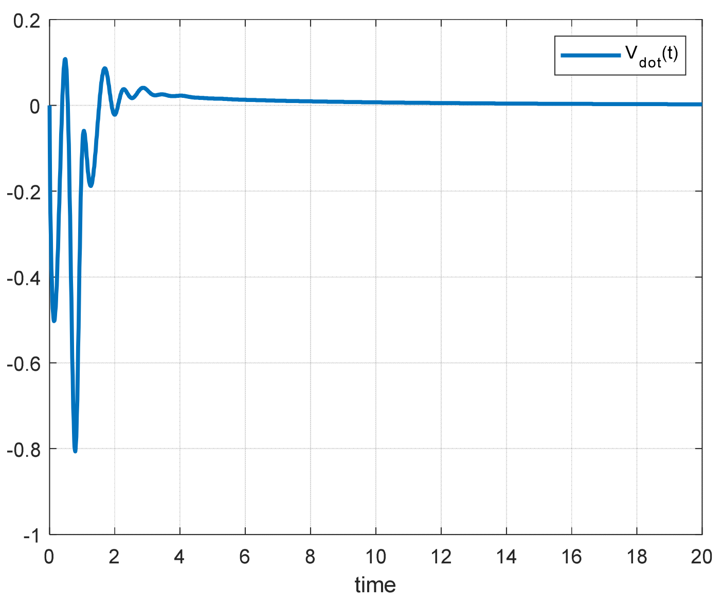
Next, we present some examples to show the behavior of the control error $e_1\left(t\right)$ and the derivative of the Lyapunov function $\dot{V}(e,\varphi )$ that confirm the convergence to zero of $e_1\left(t\right)$, which is the main result of this paper, and this was proven in the previous section.

5.1. Scalar Stable Plant

Example 1.

($n=1$and  $n^{*}=1$).

Remark 3.

In the scalar case,  ${\theta }_0^{*}={\theta }^{*}={\displaystyle \frac{a_m-a_p}{b_p}}$ and  $k^{*}={\displaystyle \frac{b_m}{b_p}}$, where  ${\theta }^{*}$ and  $k^{*}$ are the ideal control parameters and  $u\left(t\right)=k\left(t\right)r\left(t\right)+\theta \left(t\right)x_p\left(t\right)$ is the control law.

Then, using the MKY lemma, that is, for any $Q=Q^T>0$ a $P=P^T>0$ exists, such that

$$\begin{array}{l}{A}_{mn}^{T}P+P{A}_{mn}=-Q.\\ P{b}_{mn}=h_{mn}.\end{array}$$

we may calculate $A_{mn}, P$, and $Q$ for the system of Example 1 and thus be able to calculate $\dot{V}(e,\varphi )$.

In this example, $A_{mn}=-2, P=1$, $Q=2$, $k^{*}={\displaystyle \frac{b_m}{b_p}}=2$, and ${\theta }^{*}={\displaystyle \frac{a_m-a_p}{b_p}}=-1$. In

Table 1. FO-DMRAC implementation for a stable plant.

Plant Model	Reference Model
${\dot{x}}_p\left(t\right)=-x_p\left(t\right)+u\left(t\right)$. $y_p\left(t\right)=x_p\left(t\right)$. $W_p\left(s\right)={\displaystyle \frac{1}{s+1}}$. $a_p=-1, b_p=1, h_p=h_p^T=1$.	${\dot{x}}_m\left(t\right)=-2\left(t\right)+2r\left(t\right)$. $r\left(t\right)=1$. $y_m\left(t\right)=x_m\left(t\right)$. $W_m\left(s\right)={\displaystyle \frac{2}{s+2}}$. $a_m=-2, b_m=2, h_m=h_m^T=1$.
$\mathsf{\Lambda }=0, l=0, A_{mn}=-2, { b}_{mn}=-1, e\left(t\right)=e_1\left(t\right)=x_p-x_m$

the differential equations and values of Example 1 are shown.

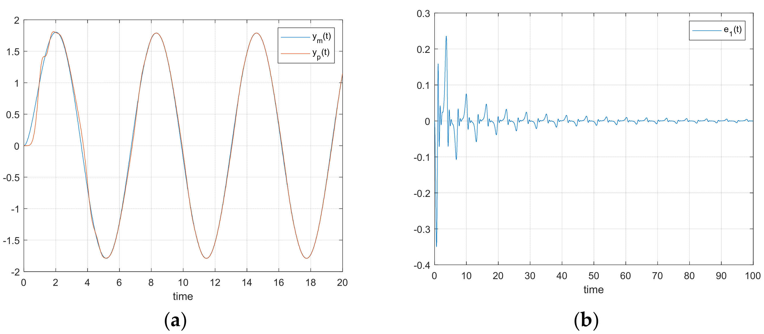
The fractional adaptive laws were implemented using the Ninteger Toolbox [23]. Specifically, the NID block was used based on the Oustaloup method [24].

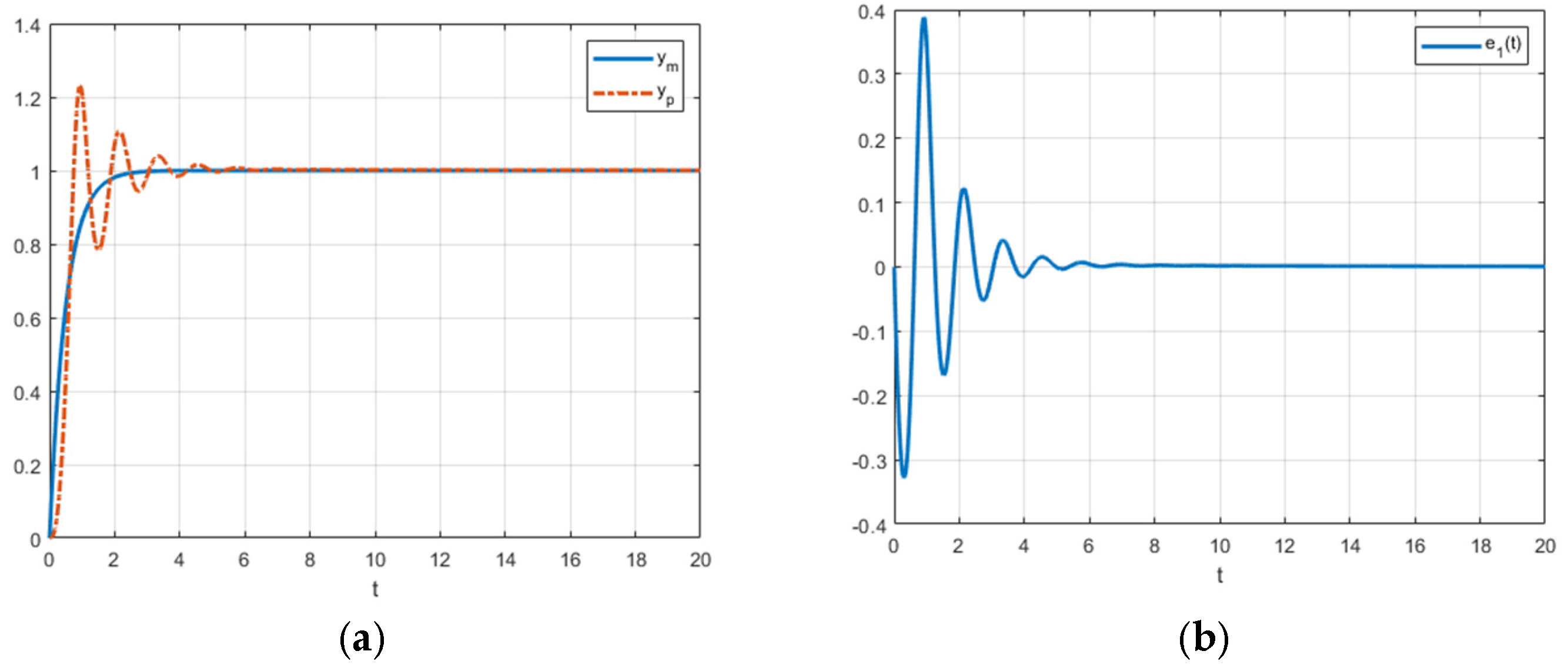
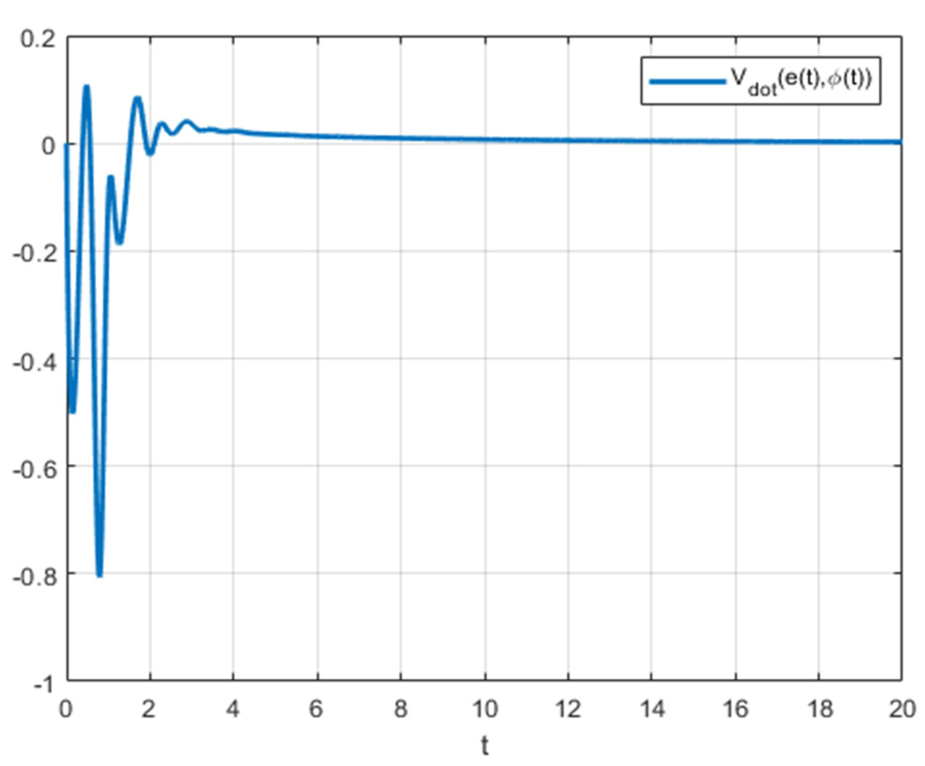
Figure 3 shows the plant response $y_p\left(t\right)$, reference output $y_m\left(t\right)$, and control error $e_1\left(t\right)$, respectively. From Figure 4, we can see the evolution of $\dot{V}(e,\varphi )$, respectively.

Additionally, as shown in Figure 3 and Figure 4, the control error $e_1\left(t\right)$ converges to zero, and while $\dot{V}(e,\varphi )$ may be greater than zero in certain time intervals, it ultimately converges to zero as $t\to \infty$, like the classical case.

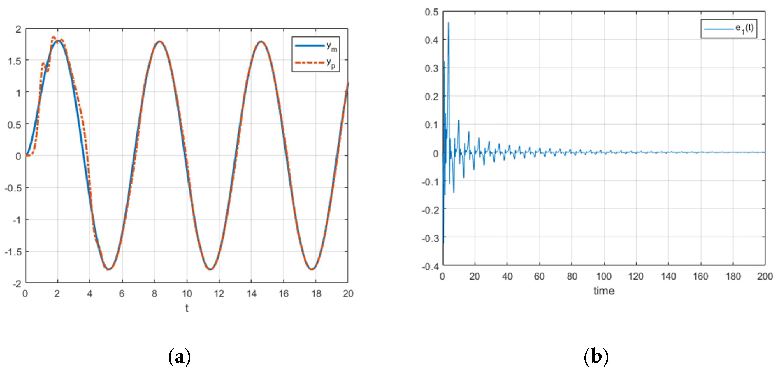
If we change $r\left(t\right)$ by a sinusoidal signal such as $r\left(t\right)=2\sin \left(t\right)$, the response, control error, and the graph of $\dot{V}(e,\varphi )$ are shown in Figure 5 and Figure 6, respectively.

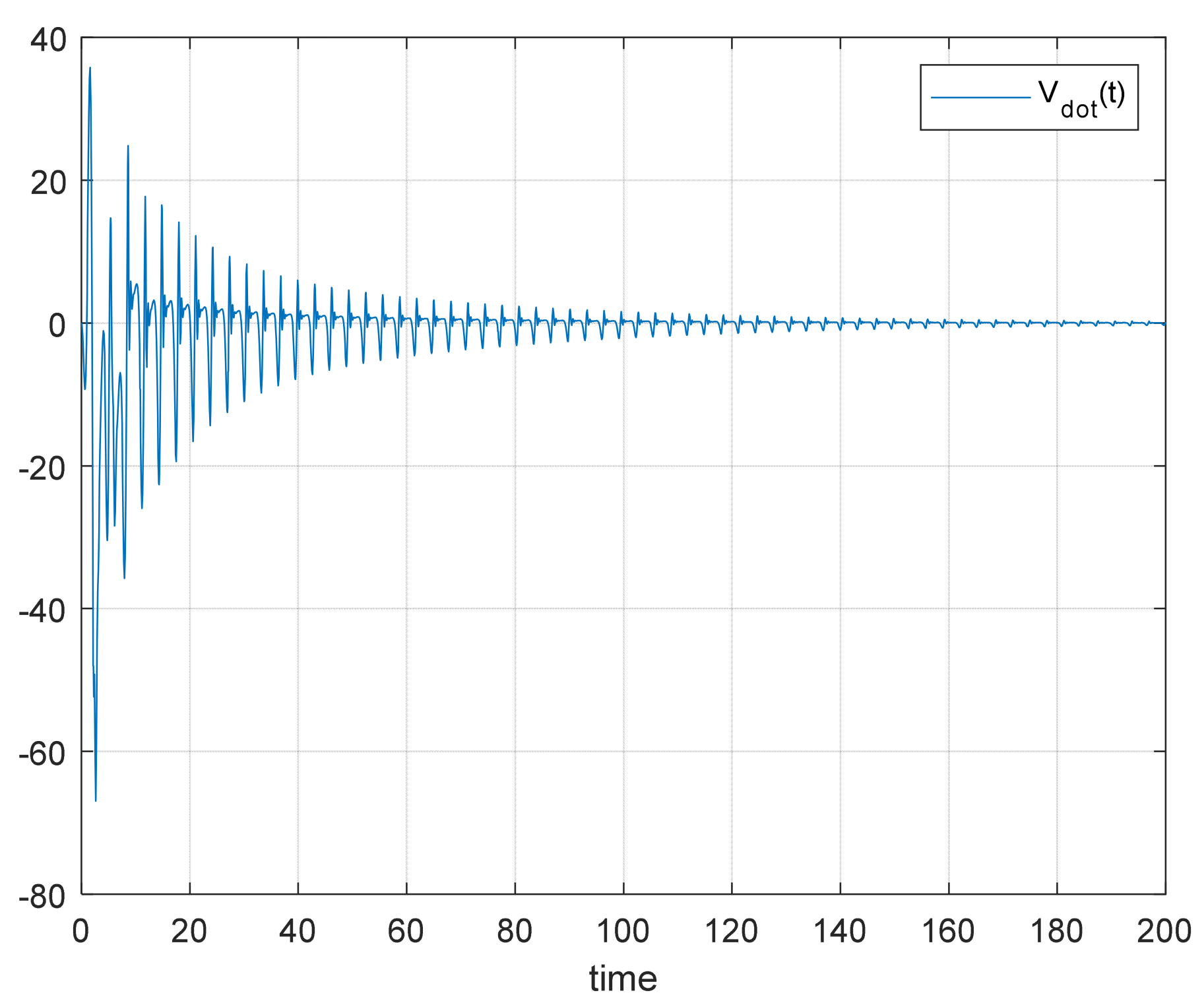
From Figure 5, the control error $e_1\left(t\right)$ convergence takes more time than the stable case, but the convergence is assured anyway. A similar convergence behavior can be seen from Figure 6.

5.2. Scalar Unstable Plant

Example 2.

($n=1$and  $n^{*}=1$).

$A_{mn}=-2, P=1$, $Q=2$, $k^{*}={\displaystyle \frac{b_m}{b_p}}=2$ and ${\theta }^{*}={\displaystyle \frac{a_m-a_p}{b_p}}=-3$. 

Table 2. FO-DMRAC implementation for an unstable plant.

Plant Model	Reference Model
${\dot{x}}_p\left(t\right)=1\left(t\right)+1u\left(t\right)$. $y_p\left(t\right)=x_p\left(t\right)$. $W_p\left(s\right)={\displaystyle \frac{1}{s-1}}$. $a_p=1, b_p=1, h_p=h_p^T=1$.	${\dot{x}}_m\left(t\right)=-2\left(t\right)+2r\left(t\right)$. $r\left(t\right)=1$. $y_m\left(t\right)=x_m\left(t\right)$. $W_m\left(s\right)={\displaystyle \frac{2}{s+2}}$. $a_m=-2, b_m=2, h_m=h_m^T=1$.
$\mathsf{\Lambda }=0, l=0, A_{mn}=-2, { b}_{mn}=-1, e\left(t\right)=e_1\left(t\right)=x_p-x_m$

shows the differential equations and values of Example 2.

The next figures (Figure 7 and Figure 8) show similar convergence behavior as the graphics of Example 1 for the unstable plant.

Now, if we change the reference to $r\left(t\right)=2\sin \left(t\right)$, the figures are as follows (Figure 9 and Figure 10).

As we can see, from Figure 10 and Figure 11, both the control error $e_1\left(t\right)$ and $\dot{V}(e,\varphi )$ converge to 0, even if $\dot{V}(e,\varphi )$ can take positive values in some time intervals.

5.3. Vectorial Case (Stable Plant)

Example 3.

($n=2$and$n^{*}=1$).

Table 3. FO-DMRAC implementation.

Plant Model	Reference Model
${\dot{x}}_p\left(t\right)=A_p\left(t\right)x_p\left(t\right)+b_{p}u\left(t\right)$. $y_p\left(t\right)=h_p^T{x}_p\left(t\right)$. $W_p\left(s\right)={\displaystyle \frac{s+1}{s^2+7s+12}}$ Controllable canonical form: $A_p=\left[\begin{array}{cc}0& 1\\ -12& -7\end{array}\right], b_p=\left[\begin{array}{c}0\\ 1\end{array}\right],$ $h_p^T=[1 1]$	${\dot{x}}_m\left(t\right)=-2\left(t\right)+2r\left(t\right)$. $y_m\left(t\right)=x_m\left(t\right)$. $r\left(t\right)=1$. $W_m\left(s\right)={\displaystyle \frac{2}{s+2}}{\displaystyle \frac{(s+1)}{(s+1)}}$ Controllable canonical form: $A_p=\left[\begin{array}{cc}0& 1\\ -2& -3\end{array}\right], b_p=\left[\begin{array}{c}0\\ 1\end{array}\right],$ $h_m^T=[1 1]$
$\mathsf{\Lambda }=-1, l=1, { b}_{mn}={\left[0 1 1 0\right]}^T, h_{mn}^T=[1 1 0 0]$ $e\left(t\right)=x\left(t\right)-x_{mn}\left(t\right)$ $e_1\left(t\right)=h_{mn}^{T}e\left(t\right)$

shows the differential equations and values of Example 3.

Remark 4.

The reference model transfer function  $W_m\left(s\right)$ has been changed (order 2) just to match the conditions for finding the control ideal parameters  ${\theta }^{*}$, but the behavior is the same as the original transfer function  $W_m\left(s\right)={\displaystyle \frac{2}{s+2}}$.

Control Laws:

$$\begin{gathered} \theta \left(t\right)={\left[\begin{array}{cc}k\left(t\right)& {\theta }_1^T\left(t\right)\end{array} \begin{array}{cc}{\theta }_0\left(t\right)& {\theta }_2^T\left(t\right)\end{array}\right]}^T\in {\mathbb{R}}^4 \\ \omega \left(t\right)={\left[\begin{array}{cc}r\left(t\right)& {\omega }_1^T\left(t\right)\end{array} \begin{array}{cc}{y}_p\left(t\right)& {\omega }_2^T\left(t\right)\end{array}\right]}^T\in {\mathbb{R}}^4 \\ u\left(t\right)={\theta }^T\left(t\right)\omega \left(t\right) \end{gathered}$$

Note: ${\theta }_1^T\left(t\right)$ and ${\theta }_2^T\left(t\right)$ $\in \mathbb{R}$

Internal auxiliary signals:

$$\begin{gathered} {\dot{\omega }}_1\left(t\right)=\mathsf{\Lambda }{\omega }_1\left(t\right)+lu\left(t\right) \\ {\dot{\omega }}_2\left(t\right)=\mathsf{\Lambda }{\omega }_2\left(t\right)+l{y}_p\left(t\right) \\ \mathsf{\Lambda }=-1 \\ l=1 \end{gathered}$$

Fractional order adaptive laws:

$${}_{t_0}{}^{C}D_t^{{\alpha }_i}\theta \left(t\right)=-{\mathsf{\Gamma }}_i{e}_1\left(t\right)\omega \left(t\right)$$

Remark 5.

${\Gamma }_i$ is a diagonal matrix where  $i=1,\dots ,4$. For practical implementation simplicity, we choose  ${\Gamma }_i=I$ (identity matrix of appropriated dimension).

$\varphi \left(t\right)=\left[\begin{array}{c}\psi \left(t\right)\\ {\varphi }_1\left(t\right)\\ {\varphi }_0\left(t\right)\\ {\varphi }_2\left(t\right)\end{array}\right]=\left[\begin{array}{c}k\left(t\right)-k^{*}\\ {\theta }_1\left(t\right)-{\theta }_1^{*}\\ {\theta }_0\left(t\right)-{\theta }_0^{*}\\ {\theta }_2\left(t\right)-{\theta }_2^{*}\end{array}\right] \in {\mathbb{R}}^4$ are the parameters error vector controllers and

${\theta }^{*}=\left[\begin{array}{c}{k}^{*}\\ {\theta }_1^{*}\\ {\theta }_0^{*}\\ {\theta }_2^{*}\end{array}\right]=\left[\begin{array}{c}2\\ 0\\ 4\\ 6\end{array}\right]$ are the ideal controller parameters.

Finally, $A_{mn}=\left[\begin{array}{c}0\\ -8\\ 4\\ 1\end{array}\begin{array}{c}1\\ -3\\ 4\\ 1\end{array}\begin{array}{c}0\\ 0\\ -1\\ 0\end{array}\begin{array}{c}0\\ 6\\ 6\\ -1\end{array}\right]$

whose eigenvalues are −1, −2, −1, and −1; therefore, $A_{mn}$ is Hurwitz. Also, if

$Q=\left[\begin{array}{c}2\\ 26.5\\ -23.5\\ -6\end{array} \begin{array}{c}26.5\\ 33\\ -16.5\\ -8\end{array} \begin{array}{c}-23.5\\ -16.5\\ 4\\ 0\end{array} \begin{array}{c}-6\\ -8\\ 0\\ 2\end{array}\right]$, which is a symmetrical and positive defined matrix, then

$P=\left[\begin{array}{c}4\\ 0.5\\ 0.5\\ 1\end{array} \begin{array}{c}0.5\\ 3\\ -2\\ 0\end{array} \begin{array}{c}0.5\\ -2\\ 2\\ 0\end{array} \begin{array}{c}1\\ 0\\ 0\\ 1\end{array}\right]$, which is also a symmetrical and positive defined matrix that satisfies the MKY Lemma. That is

$$\begin{gathered} A_{mn}^{T}P+P{A}_{mn}=-Q, \\ P{b}_{mn}=h_{mn}. \end{gathered}$$

As before, Figure 11 and Figure 12 show the response, control error $e_1\left(t\right)$ and $\dot{V}(e,\varphi )$ behavior, respectively.

Figure 11 shows similar behavior as Examples 1 and 2; that is, the plant output $y_p\left(t\right)$ converges to the model reference output $y_m\left(t\right)$, which is equivalent to saying that the control error tends to 0 as $t\to \infty$. Also, from Figure 12, we confirm that $\underset{t\to \infty }{\lim }\dot{V}\left(e,\varphi \right)=0$, even if in some time intervals (mainly in the transient period), $\dot{V}\left(e,\varphi \right)$ can be positive.

Now, by changing the reference signal to a sinusoidal one as in the previous example, that is, $r\left(t\right)=2\sin \left(t\right)$, we obtain the following dynamic behavior, which is shown in the next figures (Figure 13 and Figure 14 respectively).

Remark 6.

These simulations are made to show that  $\underset{t\to \infty }{\mathit{lim}}{e}_1\left(t\right)=0$ (the control error converges to 0) in the case of fractional order model reference adaptive control implementation (FO-DMRAC) and not to show the performance of the controllers. Better performance can be achieved by using an optimization algorithm such as PSO [25] or another one in such a way as to choose the fractional parameters ${\alpha }_i$ and adaptive gains  ${\Gamma }_i$ more conveniently.

Finally, new conditions of the Lyapunov method can be established and applied to FO-DMRAC. That is, let $V\left(e,\varphi \right)$ be a continuous and derivable function, then

• $V\left(e,\varphi \right)>0$.
• $\dot{V}\left(0,0\right)=0$.
• If $\underset{t\to \infty }{\lim }\dot{V}\left(e,\varphi \right)=0$, then, $\underset{t\to \infty }{\lim }e\left(t\right)=0$, which implies that the control error $e_1\left(t\right)$ also converges to 0.

6. Conclusions

In this article, we have proven that in the FO-DMRAC case, the control error $e_1\left(t\right)=y_p\left(t\right)-y_m\left(t\right)$ converges to 0 even if the derivative of the Lyapunov function $V(e,\varphi )$ is greater than 0 in some time intervals (mainly in the transient periods). Some examples have been presented to show the convergence of the control error $e_1\left(t\right)$ and the behavior of the function $\dot{V}(e,\varphi )$ as $t$ approaches infinity.

One of the main difficulties in carrying out the synthesis of $\dot{V}(e,\varphi )$, for simulation purposes, is that we need to compute the ideal control parameters ${\theta }^{*}$ analytically and the matrix Q explicitly, which is not an easy task when the order of the plant to control grows in order. One practical approach to determine the ideal controller parameters ${\theta }^{*}$ is to implement the controller system using a Persistent Excitation (PE) reference input signal and wait for convergence. Sometimes, it could take a long time, depending on the system order, because the higher the order, the more parameters we must compute.

In conclusion, the convergence of the state error $e\left(t\right)$ and the control error $e_1\left(t\right)$ to zero has been demonstrated for a class of fractional adaptive control systems (FO-DMRAC) using the classical Lyapunov approach, avoiding additional complexities in the analysis. Previously, it had only been established that the mean square errors converge to zero as time approaches infinity; however, the convergence of errors themselves had not been explicitly demonstrated until now.