Dynamic Analysis of a Family of Iterative Methods with Fifth-Order Convergence

Abstract

In this paper, a new class of fifth-order Chebyshev–Halley-type methods with a single parameter is proposed by using the polynomial interpolation method. The convergence order of the new method is proved. The dynamic behavior of the new method on quadratic polynomials $P\left(x\right)=(x-a)(x-b)$ is analyzed, the strange fixed points and the critical points of the operator are obtained, the corresponding parameter planes and dynamic planes are drawn, the stability and convergence of the iterative method are visualized, and some parameter values with good properties are selected. The fractal results of the new method corresponding to different parameters about polynomial $G\left(x\right)$ are plotted. Numerical results show that the new method has less computing and higher computational accuracy than the existing Chebyshev–Halley-type methods. The fractal results show the new method has good stability and convergence. The numerical results of different iteration methods are compared and agree with the results of dynamic analysis.

1. Introduction

In 1975, Mandelbrot systematically expounded the concept, content, and significance of fractal geometry for the first time [1]. Fractal theory primarily focuses on the study of non-smooth, irregular, and self-similar shapes and phenomena existing in nature and nonlinear systems. Since then, fractal geometry has emerged as an independent discipline and entered the public spotlight, finding extensive applications across various fields [2,3,4,5]. Beyond the establishment of fractal geometry, Mandelbrot’s most notable contribution is the discovery of the Mandelbrot set [6]. This set is constructed by iterating the complex function $F\left(x\right)=x^2+c$ as follows: after numerous iterations, the set comprises all non-divergent parameter values $c\in \mathbb{C}$. The iteration follows the recurrence relation $x_{n+1}=x_n^2+c$ with the default initial value $x_0=0$, and the Mandelbrot set can be formally expressed as $\{0,F(0),F(F\left(0\right)),\dots \}$. The corresponding Julia set is derived from the same iterative framework but with a key distinction as follows: for a given parameter $c\in \mathbb{C}$, the Julia set [7,8] consists of all initial points $x_0$ that remain non-divergent after repeated iterations. Mathematically, it represents the set of points x for which the sequence $\{x,x^2+c,{(x^2+c)}^2+c,\dots \}$ does not diverge.

We first review some fundamental theories related to the Julia set. Specifically, in the third section of this paper, we utilize the Scaling Theorem to prove that the iterative operator of the proposed iterative method possesses conjugacy. This conjugacy property lays a crucial theoretical foundation for the subsequent dynamical analysis of the method, as it reveals the invariant structural characteristics of the iterative operator under specific transformations, thereby facilitating the exploration of its stability and convergence behavior. Consider a polynomial $F\left(x\right)=a_0+a_{1}x+a_2{x}^2+\cdots +a_n{x}^n$ where $n\ge 2$ and $F:\mathbb{C}\to \mathbb{C}$. Define the iterates of F recursively as follows: $F^0\left(x\right)=x$, $F^1\left(x\right)=F\left(x\right)$, $F^2\left(x\right)=F\left(F\left(x\right)\right)$, …, $F^{n+1}\left(x\right)=F\left(F^n\left(x\right)\right)$. A point x satisfying $F\left(x\right)=x$ is called a fixed point of F. For a fixed point w with $F^{\prime }\left(w\right)=\beta$, the dynamical properties of w are classified as follows: (1) superattractive if $\beta =0$; (2) attractive if $0<\left|\beta \right|<1$; (3) neutral (saddle point) if $\left|\beta \right|=1$; and (4) repulsive if $\left|\beta \right|>1$. The Julia set of F can be defined as the closure of the set of repulsive periodic points of F, while the complement of the Julia set in the complex plane is known as the Fatou set [9]. With the aforementioned theoretical foundation, many scholars have applied fractal theory to investigate the stability of parameterized iterative methods in recent years, yielding significant results [10,11,12,13,14,15]. For instance, Wang et al. [16] analyzed the stability of an optimal eighth-order single-parameter King’s method using Möbius conjugate maps on the Riemann sphere. Capdevila et al. [17] introduced isonormal surfaces to study the dynamical behavior of the rational vector operator associated with a multidimensional iterative method for polynomial systems. Campos et al. [18] conducted a dynamical analysis of a memory-based iterative method applied to cubic polynomials. Cordero et al. [19] pioneered the dynamical study of a matrix iterative method, successfully identifying its stability intervals. Francisco et al. [20] carried out in-depth research on the influence of multidimensional weight functions on the stability of iterative processes. Moscoso-Martínez et al. [21] constructed stability surfaces and dynamical planes to illustrate the complex behavior of an optimal-order iterative method. The development of iterative methods for solving equations dates back to the 17th century, when Newton proposed his iconic iterative method for approximating roots in both real and complex fields. Since then, numerous improved iterative methods have been developed based on Newton’s method [22,23,24,25,26]. In 1990, building upon Newton’s method, an iterative method incorporating the second derivative was proposed, known as the Chebyshev-type iterative method [27], expressed as follows:

$$x_{n+1}=x_n-(1+{\displaystyle \frac{1}{2}}{L}_f\left(x_n\right)){\displaystyle \frac{f\left(x_n\right)}{f^{\prime }\left(x_n\right)}},$$

where

$$L_f\left(x_n\right)={\displaystyle \frac{f\left(x_n\right)f^{\prime \prime }\left(x_n\right)}{{f^{\prime }\left(x_n\right)}^2}}.$$

It is a third-order convergence. At the same time, the Halley iterative method [28] was also proposed.

$$x_{n+1}=x_n-({\displaystyle \frac{1+\frac{1}{2}{L}_f\left(x_n\right)}{1-\frac{1}{2}{L}_f\left(x_n\right)}}){\displaystyle \frac{f\left(x_n\right)}{f^{\prime }\left(x_n\right)}},$$

On the basis of the Halley-type method, a super Halley-type iteration method [29] is obtained.

$$x_{n+1}=x_n-({\displaystyle \frac{1+\frac{1}{2}{L}_f\left(x_n\right)}{1-L_f\left(x_n\right)}}){\displaystyle \frac{f\left(x_n\right)}{f^{\prime }\left(x_n\right)}},$$

In 1997, Gutierrez and Hernández [30] summarized the above three methods and obtained a third-order iterative method with parameters, called the Chebyshev–Halley-type iterative method.

$$x_{n+1}=x_n-(1+{\displaystyle \frac{L_f\left(x_n\right)}{2(1-\alpha L_f\left(x_n\right))}}){\displaystyle \frac{f\left(x_n\right)}{f^{\prime }\left(x_n\right)}}.$$

(1)

In this paper, we propose a novel two-step fifth-order parameterized Chebyshev–Halley-type iterative method derived via polynomial interpolation. The rest of this paper is organized as follows: Section 2 presents the derivation process and convergence order proof of the new method. Section 3 utilize the Scaling Theorem to prove that the iterative operator of the proposed iterative method possesses conjugacy. Section 4 analyzes the dynamical behavior of the proposed method using fractal theory. Section 5 compares the fractal patterns of the new method under different parameter settings. Section 6 provides numerical experiments comparing the new method with existing iterative methods, demonstrating its advantages in both convergence performance and stability.

2. Improved Methods and Convergence Analysis

The new method proposed in this paper is based on the Chebyshev–Halley-type iterative methods. Let us consider the following form first:

$$\left\{\begin{array}{c}{y}_n=x_n-(H_0+H_1{L}_f\left(x_n\right)+H_2{L}_f^2\left(x_n\right)){\displaystyle \frac{f\left(x_n\right)}{f^{\prime }\left(x_n\right)}},\\ \\ x_{n+1}=y_n-{\displaystyle \frac{f\left(y_n\right)}{f^{\prime }\left(y_n\right)}},\end{array}\right.$$

(2)

where

$$L_f\left(x_n\right)={\displaystyle \frac{f\left(x_n\right)f^{\prime \prime }\left(x_n\right)}{{f^{\prime }\left(x_n\right)}^2}}.$$

Using the interpolation polynomial, let

$$q\left(t\right)=A{t}^2+Bt+C,$$

(3)

where $A,B$, and C are undetermined coefficients. And the polynomial satisfies the following three conditions

$$f\left(x_n\right)=q\left(x_n\right),$$

(4)

$$f^{\prime }\left(x_n\right)=q^{\prime }\left(x_n\right),$$

(5)

$$f\left(y_n\right)=q\left(y_n\right),$$

(6)

Using the above conditions we get

$$A={\displaystyle \frac{f^{\prime \prime }\left(x_n\right)}{2}},B=f^{\prime }\left(x_n\right)-f^{\prime \prime }\left(x_n\right)x_n,C={\displaystyle \frac{1}{2}}(2f\left(y_n\right)-2f^{\prime }\left(x_n\right)x_n+f^{\prime \prime }\left(x_n\right){x_n}^2)$$

(7)

Now, we obtain

$$f^{\prime }\left(y_n\right)\approx q^{\prime }\left(y_n\right)=2A{y}_n+B=f^{\prime }\left(x_n\right)+f^{\prime \prime }\left(x_n\right)(y_n-x_n).$$

(8)

Bringing (7) into iterative format (1), we get the following iteration expression:

$$\left\{\begin{array}{c}{y}_n=x_n-(H_0+H_1{L}_f\left(x_n\right)+H_2{L}_f^2\left(x_n\right)){\displaystyle \frac{f\left(x_n\right)}{f^{\prime }\left(x_n\right)}},\\ \\ x_{n+1}=y_n-{\displaystyle \frac{f\left(y_n\right)}{f^{\prime }\left(x_n\right)+f^{\prime \prime }\left(x_n\right)(y_n-x_n)}},\end{array}\right.$$

(9)

where

$$L_f\left(x_n\right)={\displaystyle \frac{f\left(x_n\right)f^{\prime \prime }\left(x_n\right)}{{f^{\prime }\left(x_n\right)}^2}}.$$

Next, we will analyze the convergence order of this iterative method (23).

Theorem 1.

Let $\alpha \in I_f\subset D$ be a simple zero of a real single-valued function $f:D\subset R\to R$, which is continuously differentiable up to the fifth order in the neighborhood of $\alpha \in I_f$ (where $I_f$ is an open interval). If the iterative method (8) satisfies $H_0=1,H_1={\displaystyle \frac{1}{2}},H_2={\displaystyle \frac{1}{2}}+\lambda$, then it achieves fifth-order convergence, with the following error expression:

$$e_{n+1}=3c_3(4\lambda c_2^2+c_3)e_n^5+O\left({e_n}^6\right),$$

(10)

where the parameter λ is a real free parameter.

Proof. 

Let $c_n={\displaystyle \frac{f^{\left(n\right)}\left(\alpha \right)}{n!f^{\prime }\left(\alpha \right)}}$, $e_n=x_n-\alpha ,e_y=y_n-\alpha ,$ and $e_{n+1}=x_{n+1}-\alpha$. Taking the Taylor expansion of f at $\alpha$, we can get

$$f\left(x_n\right)=f^{\prime }\left(\alpha \right)(e_n+c_2{e_n}^2+c_3{e_n}^3+c_4{e_n}^4+O\left({e_n}^5\right)),$$

(11)

$$f^{\prime }\left(x_n\right)=f^{\prime }\left(\alpha \right)(1+2c_2{e}_n+3c_3{e_n}^2+4c_4{e_n}^3+O\left({e_n}^4\right)),$$

(12)

$$f^{\prime \prime }\left(x_n\right)=f^{\prime }\left(\alpha \right)(2c_2+6c_3{e}_n+12c_4{e_n}^2+O\left(e_n^3\right)).$$

(13)

From (10) and (11), we have

$$\begin{array}{cc}\hfill {\displaystyle \frac{f\left(x_n\right)}{f^{\prime }\left(x_n\right)}}=& e_n-c_2{e}_n^2+(2c_2^2-2c_3)e_n^3+(-4c_2^3+7c_2{c}_3-3c_4)e_n^4\hfill \\ \hfill +& (8c_2^4-20c_2^2{c}_3+6c_3^2+10c_2{c}_4-4c_5)e_n^5.\hfill \end{array}$$

(14)

Using (8) and (10)–(12), we have

$$\begin{array}{cc}\hfill L_f\left(x_n\right)=& {\displaystyle \frac{f\left(x_n\right)f^{\prime \prime }\left(x_n\right)}{f^{\prime }{\left(x_n\right)}^2}}\hfill \\ \hfill =& 2c_2{e}_n+(-6c_2^2+6c_3)e_n^2+4(4c_2^3-7c_2{c}_3+3c_4)e_n^3\hfill \\ \hfill -& 10(4c_2^4-10c_2^2{c}_3+3c_3^2+5c_2{c}_4-2c_5)e_n^4,\hfill \end{array}$$

(15)

And

$$\begin{array}{cc}\hfill e_y=& e_n-(H_0+H_1{L}_f\left(x_n\right)+H_2{L}_f^2\left(x_n\right)){\displaystyle \frac{f\left(x_n\right)}{f^{\prime }\left(x_n\right)}}\hfill \\ \hfill =& (1-H_0)e_n+c_2(H_0-2H_1)e_n^2+(2c_3(H_0-3H_1)-2c_2^2(H_0-4H_1+2H_2))e_n^3\hfill \\ \hfill & +(3c_4(H_0-4H_1)+c_2{c}_3(-7H_0+38H_1-24H_2)+c_2^3(4H_0-26H_1+28H_2))e_n^4\hfill \\ \hfill & -2(c_2^2{c}_3(-10H_0+83H_1-108H_2)+3c_3^2(H_0-7H_1+6H_2)\hfill \\ \hfill & +c_2{c}_4(5H_0-34H_1+24H_2)+c_2^4(4H_0-38H_1+66H_2))e_n^5+O\left({e_n}^6\right).\hfill \end{array}$$

(16)

From (11), (12), and (15), we get

$$\begin{array}{cc}\hfill f^{\prime }\left(x_n\right)+& f^{\prime \prime }\left(x_n\right)(y_n-x_n)\hfill \\ \hfill =& f^{\prime }\left(\alpha \right)-2\left(c_2{f}^{\prime }\left(\alpha \right)(-1+H_0)\right)e_n+f^{\prime }\left(\alpha \right)(c_3(3-6H_0)\hfill \\ \hfill +& 2c_2^2(H_0-2H_1))e_n^2-2\left(f^{\prime }\left(\alpha \right)\right(-5c_2{c}_3{H}_0+c_4(-2+6H_0)\hfill \\ \hfill +& 12c_2{c}_3{H}_1+2c_2^3(H_0-4H_1+2H_2)\left)\right)e_n^3+f^{\prime }\left(\alpha \right)\left(c_5\right(5\hfill \\ \hfill -& 20H_0)+2(3c_2{c}_4(3H_0-8H_1)+6c_3^2(H_0-3H_1)+c_2^2{c}_3\hfill \\ \hfill & (-13H_0+62H_1-36H_2)+c_2^4(4H_0-26H_1+28H_2)\left)\right)e_n^4+O\left(e_n^5\right).\hfill \end{array}$$

(17)

Applying Taylor expansion again, we have

$$f\left(y_n\right)=f^{\prime }\left(a\right)(e_y+c_2{e_y}^2+c_3{e_y}^3+c_4{e_y}^4+O\left({e_y}^5\right)),$$

(18)

Now, using (11)–(18), we get

$$\begin{array}{cc}\hfill e_{n+1}=& y_n-{\displaystyle \frac{f\left(y_n\right)}{f^{\prime }\left(x_n\right)+f^{\prime \prime }\left(x_n\right)(y_n-x_n)}}\hfill \\ \hfill =& c_2{M}_1{e}_n^2+M_2{e}_n^3+M_3{e}^4+\left(3c_3^2\right(3H_0^3+2H_0^4+H_0^2(-19+6H_1)\hfill \\ \hfill & -2(1+6H_1)+2H_0(7+6H_1))-2c_2{c}_4(5-7H_0^4+H_0^5+H_0^2(41-12H_1)\hfill \\ \hfill & +24H_1+H_0^3(-2+4H_1)-2H_0(17+12H_1))+2c_2^4(-4-28H_0^4+4H_0^5\hfill \\ \hfill & -66H_1-28H_1^2+H_0^3(73+16H_1)+2H_0(19+73H_1+6H_1^2-28H_2)+40H_2\hfill \\ \hfill & +8H_1{H}_2+H_0^2(-85-84H_1+12H_2))+c_2^2{c}_3(20H_0^4+4H_0^5+H_0^3(-161+16H_1)\hfill \\ \hfill & +4(5+54H_1+9H_1^2-18H_2)+H_0^2(299+60H_1+12H_2)+2H_0(-83-180H_1\hfill \\ \hfill & +6H_1^2+36H_2\left)\right))e_n^5+O\left({e_n}^6\right).\hfill \end{array}$$

(19)

where $M_1={(-1+H_0)}^2$, $M_2=(-1+H_0)(c_3(-2+4H_0+H_0^2)+2c_2^2(1-3H_0+H_0^2+2H_1))$, $M_3=(c_4(3-12H_0+6H_0^2+4H_0^3-H_0^4)+c_2{c}_3(-7+7H_0^3+2H_0^4-24H_1+H_0^2(-43+6H_1)$ $+H_0(38+24H_1))+c_2^3(-22H_0^3+4H_0^4+H_0^2(41+12H_1)+4(1+7H_1+H_1^2-2H_2)+H_0(-26-44H_1+8H_2)))$.

Obviously, through (19), we can find that the iterative method is convergent in the fifth-order when the following conditions are satisfied

$$H_0=1,H_1={\displaystyle \frac{1}{2}},H_2={\displaystyle \frac{1}{2}}+\lambda ,$$

(20)

where $\lambda$ is a complex free parameter. Finally, we can obtain two-step fifth-order iterative method and its error equation

$$e_{n+1}=3c_3(4\lambda c_2^2+c_3)e_n^5+O\left(e_n^6\right),$$

(21)

$$\left\{\begin{array}{c}{y}_n=x_n-(1+{\displaystyle \frac{1}{2}}{L}_f\left(x_n\right)+({\displaystyle \frac{1}{2}}+\lambda )L_f^2\left(x_n\right)){\displaystyle \frac{f\left(x_n\right)}{f^{\prime }\left(x_n\right)}},\\ \\ x_{n+1}=y_n-{\displaystyle \frac{f\left(y_n\right)}{f^{\prime }\left(x_n\right)+f^{\prime \prime }\left(x_n\right)(y_n-x_n)}},\end{array}\right.$$

(22)

where

$$L_f\left(x_n\right)={\displaystyle \frac{f\left(x_n\right)f^{\prime \prime }\left(x_n\right)}{{f^{\prime }\left(x_n\right)}^2}}.$$

□

Remark 1.

The Chebyshev–Halley-type iterative method (1) involves three functional evaluations and achieves third-order convergence. Its computational efficiency index [31] is $3^{{\displaystyle \frac{1}{3}}}\approx 1.4422$. Compared with Method (1), the proposed new method (22) only requires one additional functional evaluation, while its convergence order is enhanced from third-order to fifth-order. The computational efficiency index of the new method is $5^{{\displaystyle \frac{1}{4}}}\approx 1.495$, which is significantly higher than that of Method (1). The parameter λ in (20) is a complex free parameter, which does not affect the convergence order of the iterative method (21). However, when the parameter takes different values, the iterative method has different structures and different stability properties. In the next section, we will analyze the influence of the parameter on the stability of the iterative method through the theory of dynamical systems.

3. Fundamentals of Analysis

The above iterative method (21) can be simply written in the following form

$$x_{n+1}=R_f\left(x_n\right),$$

(23)

$R_f\left(x_n\right)$ in (22) is called the fixed point operator or rational function of iterative family (21) which is a discrete dynamic system.

Theorem 2

(The Scaling Theorem). Let $f\left(z\right)$ be an analytic function on the Riemann sphere, and let $T\left(z\right)=az+b,a\ne 0$ be an affine map. If $h\left(z\right)=f\circ T\left(z\right)$, then $T\circ R_h\circ T^{-1}\left(z\right)=R_f\left(z\right)$, that is, the rational function $R_f$ in (23) is analytically conjugated to $R_h$ by T, where

$$R_f\left(z\right)=z-[1+{\displaystyle \frac{1}{2}}{L}_f\left(z\right)+({\displaystyle \frac{1}{2}}+\lambda )L_f^2\left(z\right)]{\displaystyle \frac{f\left(z\right)}{f^{\prime }\left(z\right)}}-{\displaystyle \frac{f\left(y_1\right)}{f^{\prime }\left(z\right)+f^{\prime \prime }\left(z\right)(y_1-z)}},$$

(24)

$$R_h\left(z\right)=z-[1+{\displaystyle \frac{1}{2}}{L}_h\left(z\right)+({\displaystyle \frac{1}{2}}+\lambda )L_h^2\left(z\right)]{\displaystyle \frac{h\left(z\right)}{h^{\prime }\left(z\right)}}-{\displaystyle \frac{h\left(y_2\right)}{h^{\prime }\left(z\right)+h^{\prime \prime }\left(z\right)(y_2-z)}},$$

(25)

$$y_1=z-[1+{\displaystyle \frac{1}{2}}{L}_f\left(z\right)+({\displaystyle \frac{1}{2}}+\lambda )L_f^2\left(z\right)]{\displaystyle \frac{f\left(z\right)}{f^{\prime }\left(z\right)}},$$

(26)

$$y_2=z-[1+{\displaystyle \frac{1}{2}}{L}_h\left(z\right)+({\displaystyle \frac{1}{2}}+\lambda )L_h^2\left(z\right)]{\displaystyle \frac{h\left(z\right)}{h^{\prime }\left(z\right)}}.$$

(27)

Proof. 

From $T\left(z\right)=az+b,a\ne 0$, and $h\left(z\right)=f\circ T\left(z\right)$, we obtain that

$$T^{-1}\left(z\right)={\displaystyle \frac{z-b}{a}}.$$

(28)

$$h\circ T^{-1}\left(z\right)=f\left(z\right),$$

(29)

$$h^{\prime }\left(T^{-1}\left(z\right)\right)=a{(h\circ T^{-1})}^{\prime }\left(z\right)=a{f}^{\prime }\left(z\right).$$

(30)

$$h^{\prime \prime }\left(T^{-1}\left(z\right)\right)=a^2{f}^{\prime \prime }\left(z\right).$$

(31)

$$L_h\left(T^{-1}\left(z\right)\right)={\displaystyle \frac{h\left(T^{-1}\left(z\right)\right)h^{\prime \prime }\left(T^{-1}\left(z\right)\right)}{h^{\prime }{\left(T^{-1}\left(z\right)\right)}^2}}={\displaystyle \frac{f\left(z\right)f^{\prime \prime }\left(z\right)}{f^{\prime }{\left(z\right)}^2}}=L_f\left(z\right).$$

(32)

Using (27)–(30), we obtain

$$\begin{array}{cc}{y}_2\left(T^{-1}\left(z\right)\right)\hfill & =T^{-1}\left(z\right)-[1+{\displaystyle \frac{1}{2}}{L}_h\left(T^{-1}\left(z\right)\right)+({\displaystyle \frac{1}{2}}+\lambda L_h^2\left(T^{-1}\left(z\right)\right))]{\displaystyle \frac{h\left(T^{-1}\left(z\right)\right)}{h^{\prime }\left(T^{-1}\left(z\right)\right)}}\\ & ={\displaystyle \frac{z-b}{a}}-[1+{\displaystyle \frac{1}{2}}{L}_f\left(z\right)+({\displaystyle \frac{1}{2}}+\lambda L_f^2\left(z\right))]{\displaystyle \frac{f\left(z\right)}{a{f}^{\prime }\left(z\right)}}\hfill \\ & ={\displaystyle \frac{y_1-b}{a}}\hfill \end{array}$$

(33)

Furthermore,

$$\begin{array}{cc}{R}_h\left(T^{-1}\left(z\right)\right)\hfill & =y_2\left(T^{-1}\left(z\right)\right)-{\displaystyle \frac{h\left(T^{-1}\left(z\right)\right)}{h^{\prime }\left(T^{-1}\left(z\right)\right)+h^{\prime \prime }\left(T^{-1}\left(z\right)\right)(y_2-T^{-1}\left(z\right))}}\\ & ={\displaystyle \frac{y_1-b}{a}}-{\displaystyle \frac{1}{a}}{\displaystyle \frac{f\left(y_1\right)}{f^{\prime }\left(z\right)+f^{\prime \prime }\left(z\right)(y_1-z)}}\hfill \\ & ={\displaystyle \frac{1}{a}}[y_1-{\displaystyle \frac{f\left(y_1\right)}{f^{\prime }\left(z\right)+f^{\prime \prime }\left(z\right)(y_1-z)}}-b]\hfill \end{array}$$

(34)

Eventually,

$$T\left(R_h\left(T^{-1}\left(z\right)\right)\right)=y_1-{\displaystyle \frac{f\left(y_1\right)}{f^{\prime }\left(z\right)+f^{\prime \prime }\left(z\right)(y_1-z)}}=R_f\left(z\right).$$

Then this proof is completed. □

The above theorem shows that it allows us to conjugate the dynamic behavior of one operator with another related rational function via an affine conjugation.

Definition 1.

Let $\mathcal{R}:\mathrm{X}\subset \overline{\mathcal{C}}\to \mathrm{X}$ and $\mathcal{O}:\mathrm{Y}\subset \overline{\mathcal{C}}\to \mathrm{Y}$ be two functions (represent two dynamical systems). We say that $\mathcal{R}$ is conjugate to $\mathcal{O}$ via T if there exists an isomorphism $T:\mathrm{Y}\to \mathrm{X}$ such that $\mathcal{R}\circ T=T\circ \mathcal{O}$. Such a map T is called a conjugacy [15,16].

According to Theorem of 3 which has been proved in Reference [16], we discover two important properties about dynamical systems, that is, the fixed-point property remains invariant under a topological conjugacy T and the Poincaré characteristic multiplier [19] of the fixed point is invariant under diffeomorphic conjugacy T.

Furthermore, we discover $\mathcal{R}=T\circ \mathcal{O}\circ T^{-1}$ and ${\mathcal{R}}^n=(T\circ \mathcal{O}\circ T^{-1})\circ (T\circ \mathcal{O}\circ T^{-1})\dots \circ (T\circ \mathcal{O}\circ T^{-1})=T\circ {\mathcal{O}}^n\circ T^{-1}$. If $\mathcal{R}$ and $\mathcal{O}$ are extra invertible, we can also find ${\mathcal{R}}^{-1}=T\circ {\mathcal{O}}^{-1}\circ T^{-1}$ and ${\mathcal{R}}^{-n}=T\circ {\mathcal{O}}^{-n}\circ T^{-1}$, besides the topological conjugacy T that maps an orbit

$$\cdots ,{\mathcal{O}}^{-2}\left(y\right),{\mathcal{O}}^{-1}\left(y\right),y,\mathcal{O}\left(y\right),{\mathcal{O}}^2\left(y\right),\cdots$$

Of $\mathcal{O}$ onto an orbit

$$\cdots ,{\mathcal{R}}^{-2}\left(x\right),{\mathcal{R}}^{-1}\left(x\right),x,\mathcal{R}\left(x\right),{\mathcal{R}}^2\left(x\right),\cdots$$

Of $\mathcal{R}$, where $x=T\left(y\right)$. From this we find the order of points is preserved. Thus, the orbits of the two maps behave similarly under homeomorphism T, that is, conjugation does not produce qualitative changes to the dynamics of the family.

Based on the invariant properties of the fixed point, the multiplier as well as the scaling theorem, it is assuredly value to study the dynamics of a conjugated map if simplified through conjugacy T.

4. Dynamical Analysis

In this part, we analyze the stability of iterative methods by observing their dynamic behavior. Therefore, the more stable members in the iterative family are selected. First of all, we bring the iterative method into the quadratic polynomial $p\left(x\right)=(x-a)(x-b)$, and through Mobius transformation, we can get a rational operator. Then, we can study the behavior characteristics of iterative methods on quadratic polynomials through the fixed points and critical points of operators. Further, taking these critical points as initial points, we can plot some corresponding parameter planes, where the range of parameters with good convergence behavior can be observed, and some relatively stable parameter values can be selected. Finally the dynamic planes associated with these good parameters are plotted.

If we consider the quadratic polynomial $p\left(x\right)$, by applying iterative method (21) to $p\left(x\right)=(x-a)(x-b)$, then we can get operator $R_p(x;a,b,\lambda )$. The operator contains three parameters, which is not conducive to our later analysis, so we introduce the Mobius transformation

$$M\left(x\right)={\displaystyle \frac{x-a}{x-b}},$$

(35)

And its inverse function

$$M^{-1}\left(x\right)={\displaystyle \frac{bx-a}{x-1}}.$$

(36)

$M\left(x\right)$ has the following properties

$$M(\infty )=1,M\left(a\right)=0,M\left(b\right)=\infty .$$

(37)

By combining $M,R_p$, and $M^{-1}$, we can get rational operators

$${\mathcal{O}}_p(x;\lambda )=(M\circ R_p\circ M^{-1})(x;\lambda )={\displaystyle \frac{x^6{(-4\lambda +x(5+4x+x^2))}^2}{{(1+4x+5x^2-4\lambda x^3)}^2}}$$

(38)

We can observe that operator ${\mathcal{O}}_p(x;\lambda )$ contains only one free parameter $\lambda$, which will greatly simplify our subsequent analysis. When special parameter values are taken, the format of the rational operators is simplified. For example,

$${\mathcal{O}}_p(x;-{\displaystyle \frac{1}{2}})={\displaystyle \frac{x^6{(2+x)}^2}{{(1+2x)}^2}}$$

$${\mathcal{O}}_p(x;0)={\displaystyle \frac{x^8{(5+4x+x^2)}^2}{{(1+4x+5x^2)}^2}}$$

4.1. Fixed Point and Critical Point

In this part, we can find the corresponding fixed points and critical points according to the rational operators above. The stability of fixed point is analyzed according to related concepts.

4.1.1. Fixed Point and Its Stability

From the definition of a fixed point, we know that the roots of the polynomial ${\mathcal{O}}_p\left(x\right)=x$ are the fixed points of operator ${\mathcal{O}}_p\left(x\right)$. If we simplify ${\mathcal{O}}_p\left(x\right)=x$, we get

$${\mathcal{O}}_p(x;\lambda )-x={\displaystyle \frac{x(x-1)\mathcal{A}(x;\lambda )}{\mathcal{B}(x;\lambda )}},$$

(39)

where

$$\begin{array}{cc}\hfill \mathcal{A}(x;\lambda )=& 1+9x+35x^2+(75-8\lambda )x^3+(100-40\lambda )x^4+(100-80\lambda -16{\lambda }^2)x^5\hfill \\ \hfill & +(100-40\lambda )x^6+(75-8\lambda )x^7+35x^8+9x^9+x^{10},\hfill \end{array}$$

(40)

$$\mathcal{B}(x;\lambda )={(1+4x+5x^2-4\lambda x^3)}^2.$$

(41)

Obviously we know that the fixed points are $x=0,x=\infty ,x=1$ and the roots of $\mathcal{A}(x;\lambda )=0$. A fixed point different from the root of the polynomial $p\left(x\right)=(x-a)(x-b)$ is called a strange fixed point. $x=0,x=\infty ,x=1$ does not depend on the value of the argument, so next we will analyze the case of the root of $\mathcal{A}(x;\lambda )=0$.

Theorem 3.

${\mathcal{O}}_p(x;\lambda )=x$ has eleven strange fixed points roots, except in the following two cases:

• If $\lambda =-{\displaystyle \frac{1}{2}}$, ${\mathcal{O}}_p(x;\lambda )-x$ can be reduced to $(-1+x)x(1+5x+9x^2+9x^3+9x^4+5x^5+x^{6}e)/{(1+2x)}^2$, and then the operator has seven strange fixed points $x=1$, $x=-2.12514\pm 0.467781i,x=-0.448812\pm 0.0987916i,x=0.0739495\pm 0.997262i$
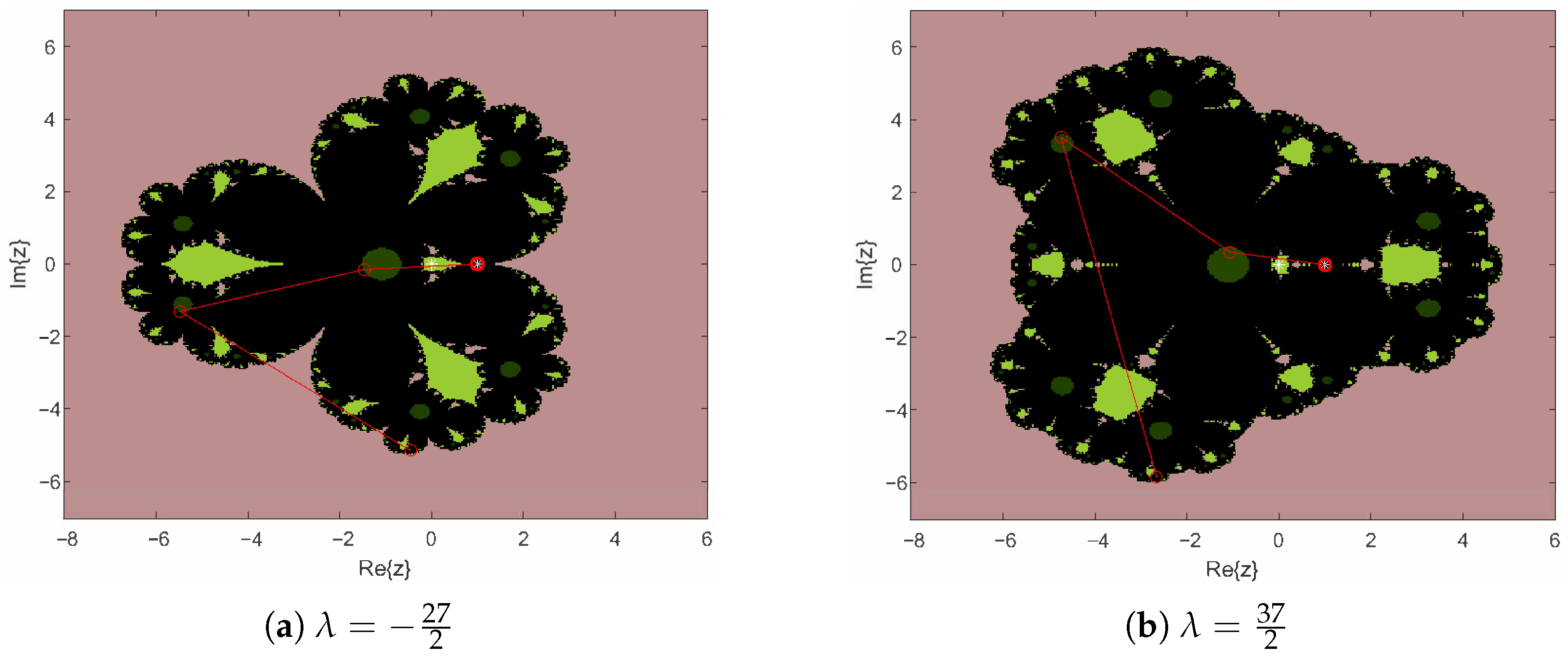
• If $\lambda =-{\displaystyle \frac{27}{2}}$, ${\mathcal{O}}_p(x;\lambda )-x$ can be reduced to $\left({(-1+x)}^{3}x(1+11x+56x^2+284x^3+1152x^4+284x^5+56x^6+11x^7+x^8)\right)/{(1+4x+5x^2+54x^3)}^2$, and then the operator has nine strange fixed points $x=1$, $x=-5.96127\pm 2.24838i,x=-0.146858\pm 0.0553897i$, $x=0.0219934\pm 0.192455i,x=0.586139\pm 5.12904i$.

Proof. 

Let us think about common factors of $\mathcal{A}(x;\lambda )$ and $\mathcal{B}(x;\lambda )$. First, let $\mathcal{A}(x;\lambda )=0$ and $\mathcal{B}(x;\lambda )=0$; then we get $(x-1){(x+1)}^{10}$ by eliminating the parameters $\lambda$, and then $(x-1),(x+1)$ is the common factor of $\mathcal{A}(x;\lambda )$ and $\mathcal{B}(x;\lambda )$. Next, by plugging $x=-1$ into ${\displaystyle \frac{\mathcal{A}(x;\lambda )}{\mathcal{B}(x;\lambda )}}=0$, we get $\lambda =-{\displaystyle \frac{1}{2}}$, where the operator ${\mathcal{O}}_p\left(x\right)$ has seven strange fixed points. Similarly, by plugging $x=1$ into ${\displaystyle \frac{\mathcal{A}(x;\lambda )}{\mathcal{B}(x;\lambda )}}=0$, we get $\lambda =-{\displaystyle \frac{27}{2}}$, in which case ${\mathcal{O}}_p\left(x\right)$ has nine strange fixed points. □

Next, we will analyze the stability of the above fixed points. We will use the first derivative of the operator ${\mathcal{O}}_p(x;\lambda )$, whose expression is as follows:

$${\mathcal{O}}_p^{\prime }(x;\lambda )={\displaystyle \frac{8x^5{(1+x)}^4(3\lambda -5x-4\lambda x+3\lambda x^2)(-4\lambda +5x+4x^2+x^3)}{{(-1-4x-5x^2+4\lambda x^3)}^3}},$$

(42)

By plugging $x=0,x=\infty$ into ${\mathcal{O}}_p^{\prime }(x;\lambda )$, we get $|{\mathcal{O}}_p^{\prime }(x;\lambda )|=0$, and then $x=0$ and $x=\infty$ are superattractive fixed points. Next we will focus on the stability analysis of other strange fixed points.

Theorem 4.

The stabilities of the fixed point $x=1$ are shown below ($\lambda \in \mathbb{C},\lambda \ne {\displaystyle \frac{5}{2}}$):

• If $|\lambda -{\displaystyle \frac{5}{2}}|>16$, $x=1$ is an attractive point;
• If $|\lambda -{\displaystyle \frac{5}{2}}|=16$, $x=1$ is a parabolic point;
• If $|\lambda -{\displaystyle \frac{5}{2}}|<16$, $x=1$ is a repulsive point.

Proof. 

By plugging $x=1$ into operator ${\mathcal{O}}_p^{\prime }\left(x\right)$, we get

$$|{\mathcal{O}}_p^{\prime }(1;\lambda )|=|{\displaystyle \frac{32}{5-2\lambda }}|$$

Let $\lambda =m+ni$ be an arbitrary complex; if we put it into $|{\displaystyle \frac{32}{5-2\lambda }}|<1$ and simplify it, we get

$$\left|32\right|<|5-(2m+2ni\left)\right|$$

Further, we get

$${(5-2m)}^2+4n^2>{32}^2$$

And by simplifying it becomes

$${(m-{\displaystyle \frac{5}{2}})}^2+n^2>{16}^2$$

Finally, we can find that when $|\lambda -{\displaystyle \frac{5}{2}}| >16$, $x=1$ is the attractive point. Similarly, when $|\lambda -{\displaystyle \frac{5}{2}}| =16$, $x=1$ is the parabolic point; when $|\lambda -{\displaystyle \frac{5}{2}}| <16$, $x=1$ is the repulsive fixed point. □

Figure 1 shows the stability of the fixed point $x=1$, as described in Theorem 4.

Figure 1. Stability region of z = 1.

Proposition 1.

We call the other strange fixed points $e{x}_i,i=1,2,\dots ,10$, which are the ten roots of the polynomial $\mathcal{A}(x;\lambda )=0$. Their stability is as follows:

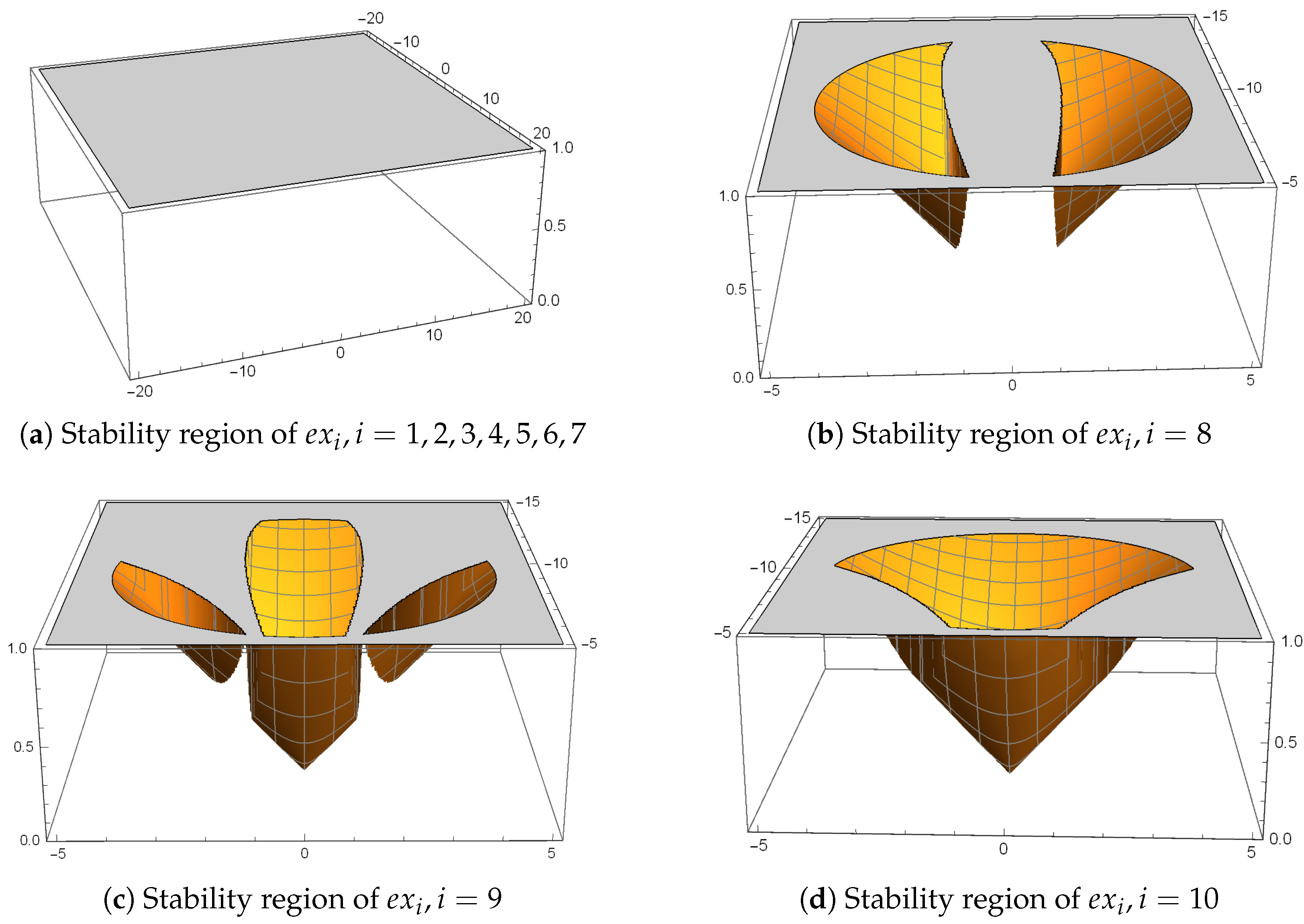
• $e{x}_i,i=1,2,3,4,5,6,7$ are all repulsive points;
• $e{x}_i,i=8,9,10$ are attractive points in the yellow area of Figure 2.

Figure 2. Stability region of $e{x}_i$.

4.1.2. Critical Point of Operator ${\mathcal{O}}_p\left(x\right)$

From the definition of the critical point, the solution of ${\mathcal{O}}_p\left(x\right)=0$ is called the critical point. When a critical point is not a root of the quadratic polynomial $p\left(x\right)=(x-a)(x-b)$, it is called a free critical point. We know from (42) that $x=0$ and $x=\infty$ are critical points, and they are also superattractive fixed points. The other critical points, $x=-1$ and the roots of the polynomial $\mathcal{F}\left(x\right)=(3\lambda -5x-4\lambda x+3\lambda x^2)(-4\lambda +5x+4x^2+x^3)=0$, are free critical points. The following will focus on analyzing the relationship between the number of free critical points and the values of parameter $\lambda$.

Theorem 5.

Operator ${\mathcal{O}}_p\left(x\right)$ has six free critical points, except in the following four cases:

• If $\lambda ={\displaystyle \frac{5}{2}}$, ${\mathcal{O}}_p\left(x\right)$ has three free critical points $x=-1,x=-2.5\pm 1.93649i$;
• If $\lambda =-{\displaystyle \frac{1}{2}}$, ${\mathcal{O}}_p\left(x\right)$ has two free critical points $x=-1,x=-2$;
• If $\lambda =-{\displaystyle \frac{25}{54}}$, ${\mathcal{O}}_p\left(x\right)$ has three free critical points $x=-1,x=-{\displaystyle \frac{3}{2}},x=-{\displaystyle \frac{5}{3}}$;
• If $\lambda =0$, ${\mathcal{O}}_p\left(x\right)$ has three free critical points $x=-1,x=-2\pm i$.

Proof. 

Let $\mathcal{G}\left(x\right)={(-1-4x-5x^2+4\lambda x^3)}^3$; similar to the proof of Theorem 3, we obtain the common factors of $\mathcal{F}\left(x\right)$ and $\mathcal{G}\left(x\right)$ by eliminating the parameter $\lambda$. The common factors are $(x-1),(x+1)$ and $(5x+3)$.

First we put $x=1$ into ${\displaystyle \frac{\mathcal{F}\left(x\right)}{\mathcal{G}\left(x\right)}}$, we get ${\displaystyle \frac{-50+40\lambda -8{\lambda }^2}{{(-10+4\lambda )}^3}}=0$, and then we get $\lambda ={\displaystyle \frac{5}{2}}$. Next, we bring $\lambda ={\displaystyle \frac{5}{2}}$ into ${\mathcal{O}}_p\left(x\right)$, and then the operator format will be reduced to ${\displaystyle \frac{60x^5{(1+x)}^4(10+5x+x^2)}{{(1+5x+10x^2)}^3}}$. So the ${\mathcal{O}}_p\left(x\right)$ has three free critical points. Similarly, by plugging $x=-1$ and $x=-{\displaystyle \frac{3}{5}}$ into ${\displaystyle \frac{\mathcal{F}\left(x\right)}{\mathcal{G}\left(x\right)}}$, we get $\lambda =-{\displaystyle \frac{1}{2}}$ and $\lambda =-{\displaystyle \frac{25}{54}}$, respectively. In this case, the corresponding ${\mathcal{O}}_p\left(x\right)$ can be reduced to ${\displaystyle \frac{12x^5{(1+x)}^2(2+x)}{{(1+2x)}^3}}$,${\displaystyle \frac{540x^5{(1+x)}^4(2+3x){(5+3x)}^3}{{(3+2x)}^3{(3+5x)}^5}}$. In this way, other conclusions of Theorem 5 can be proved. □

The expression of the free critical points ($c{r}_j,j=1,2,3,4,5,6$) are given below ($\lambda \in x(x-{\displaystyle \frac{5}{2}})(x+{\displaystyle \frac{1}{2}})(x+{\displaystyle \frac{25}{54}})\ne 0$):

$$\begin{array}{c}c{r}_1=-1;\hfill \\ c{r}_2={\displaystyle \frac{5+4\lambda -\sqrt{5}\sqrt{5+8\lambda -4{\lambda }^2}}{6\lambda }};\hfill \\ c{r}_3={\displaystyle \frac{5+4\lambda +\sqrt{5}\sqrt{5+8\lambda -4{\lambda }^2}}{6\lambda }}={\displaystyle \frac{1}{c{r}_2}};\hfill \\ c{r}_4=-{\displaystyle \frac{4}{3}}+{\displaystyle \frac{1}{3{\gamma }^{\frac{1}{3}}}}+{\displaystyle \frac{1}{3}}{\gamma }^{{\displaystyle \frac{1}{3}}};\hfill \\ c{r}_5=-{\displaystyle \frac{4}{3}}-{\displaystyle \frac{1+i\sqrt{3}}{6{\gamma }^{\frac{1}{3}}}}+{\displaystyle \frac{1}{6}}(1-i\sqrt{3}){\gamma }^{{\displaystyle \frac{1}{3}}};\hfill \\ c{r}_6=-{\displaystyle \frac{4}{3}}-{\displaystyle \frac{1-i\sqrt{3}}{6{\gamma }^{\frac{1}{3}}}}+{\displaystyle \frac{1}{6}}(1+i\sqrt{3}){\gamma }^{{\displaystyle \frac{1}{3}}},\hfill \end{array}$$

where $\gamma \left(\lambda \right)=26+54\lambda +3\sqrt{3}\sqrt{25+104\lambda +108{\lambda }^2}$.

4.2. Parameter Spaces and Dynamic Planes

In this part, we study the parameter spaces and dynamic planes associated with the iterative methods. Taking the critical points as the initial point, the corresponding parameter spaces can be drawn, and the convergence of the iterative methods corresponding to the parameters can be seen intuitively in the parameter spaces. Thus some parameters with better results can be selected. Next, we select some special parameters according to the parameter space, such as some parameter values that converge to 0 and ∞, some parameter values that converge to other roots, and some other parameter values that appear in Theorem 5. Using these parameter values, the relevant dynamic planes are plotted and their convergence can be observed.

4.2.1. Parameter Space

In Section 4.1.2, we have calculated all the free critical points; in this part, we use these free critical points to plot the corresponding parameter plane. Where $x=-1$ is the pre-image of the fixed point $x=1$, and the features of the relevant parameter plane of $x=-1$ are not significant, we do not draw the relevant parameter plane. In this way, we focus on other critical points of freedom. We already know $c{r}_2={\displaystyle \frac{1}{c{r}_3}}$ and their parameter plane effects are similar, so we can choose one of them as the initial point to draw the parameter plane for our study. Then, we can also choose $c{r}_4$ as the initial point to draw the parameter plane. Finally, in this section, two different parameter planes are studied.

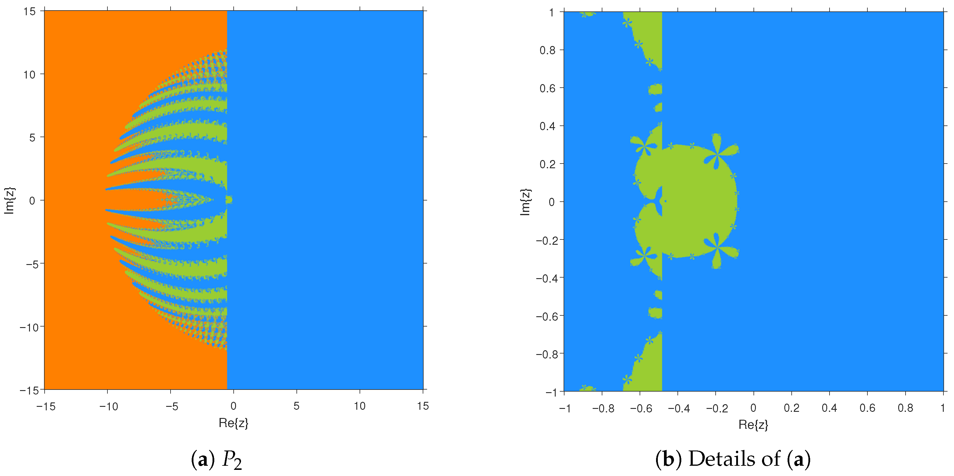
When drawing the parameter space, convergence to 0 is blue, convergence to infinity is green, and convergence to other roots is orange. These figures are plotted with a mesh of $1000\times 1000$ points and 50 iterations per point. Using the above principles, we draw the parameter plane $P_1$ and $P_2$ with $c{r}_2$ and $c{r}_4$ as the initial points, respectively, to get Figure 3 and Figure 4.

Figure 3. Parameter space $P_1$.

Figure 4. Parameter space $P_2$.

Three colors appear in Figure 3 and Figure 4, indicating that they converge not only to 0 and infinity but also to other roots. We do not want our iterative methods to converge to other roots. Therefore, when selecting parameters, the results obtained by selecting parameters in the blue and green areas will be better.

4.2.2. Dynamic Planes

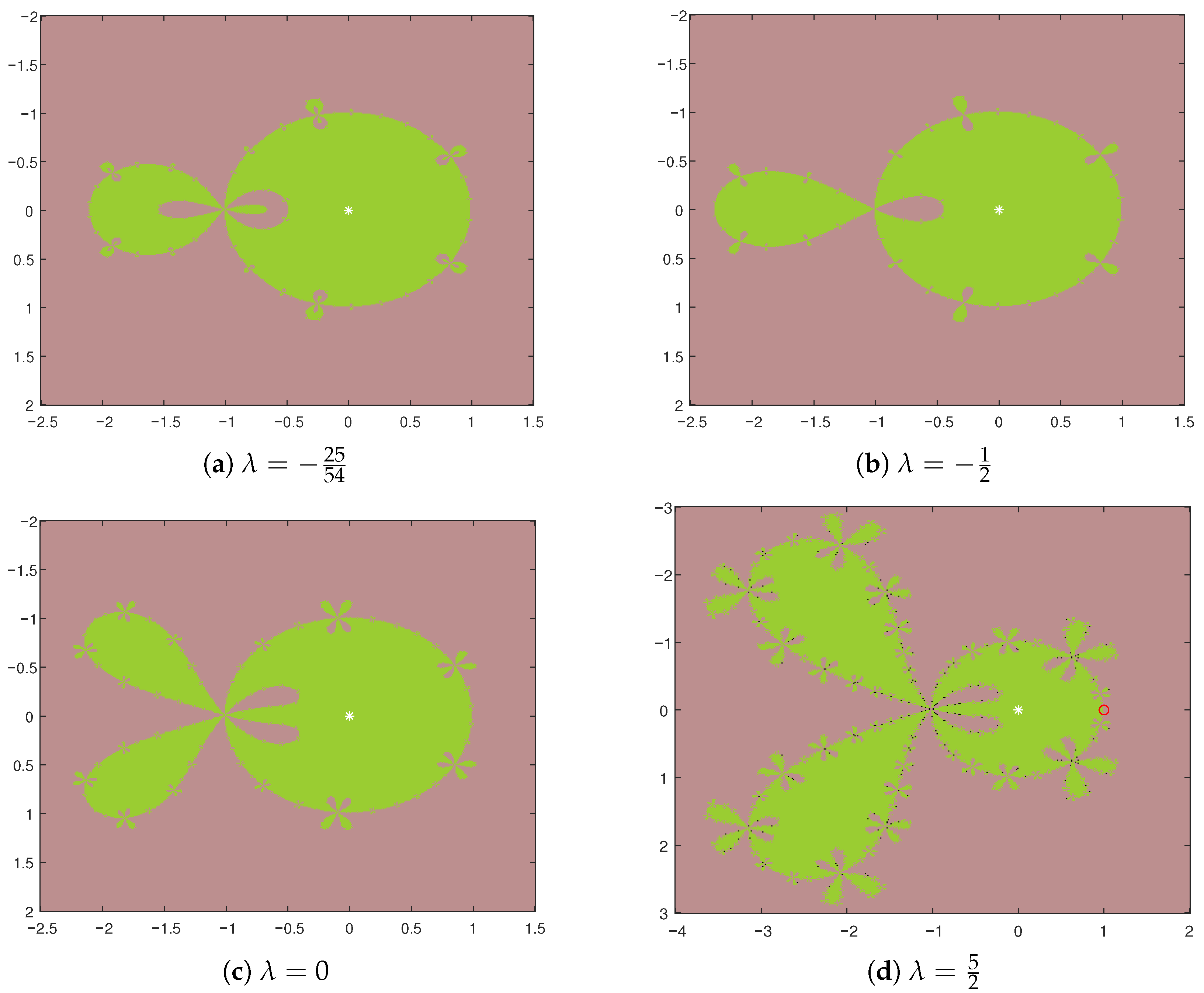
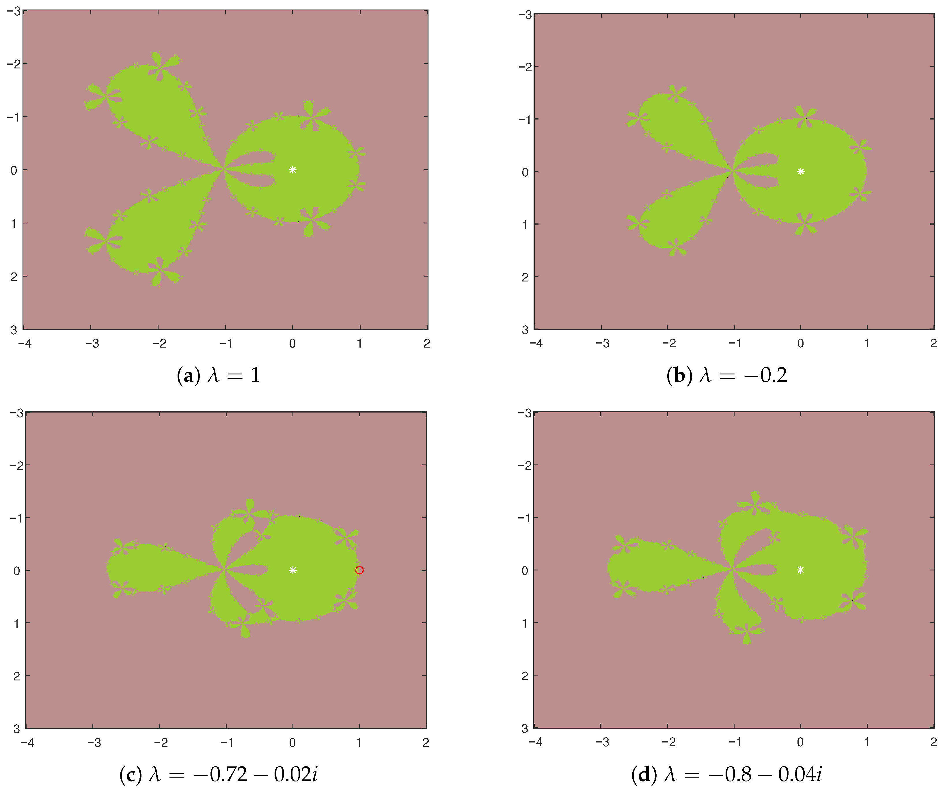
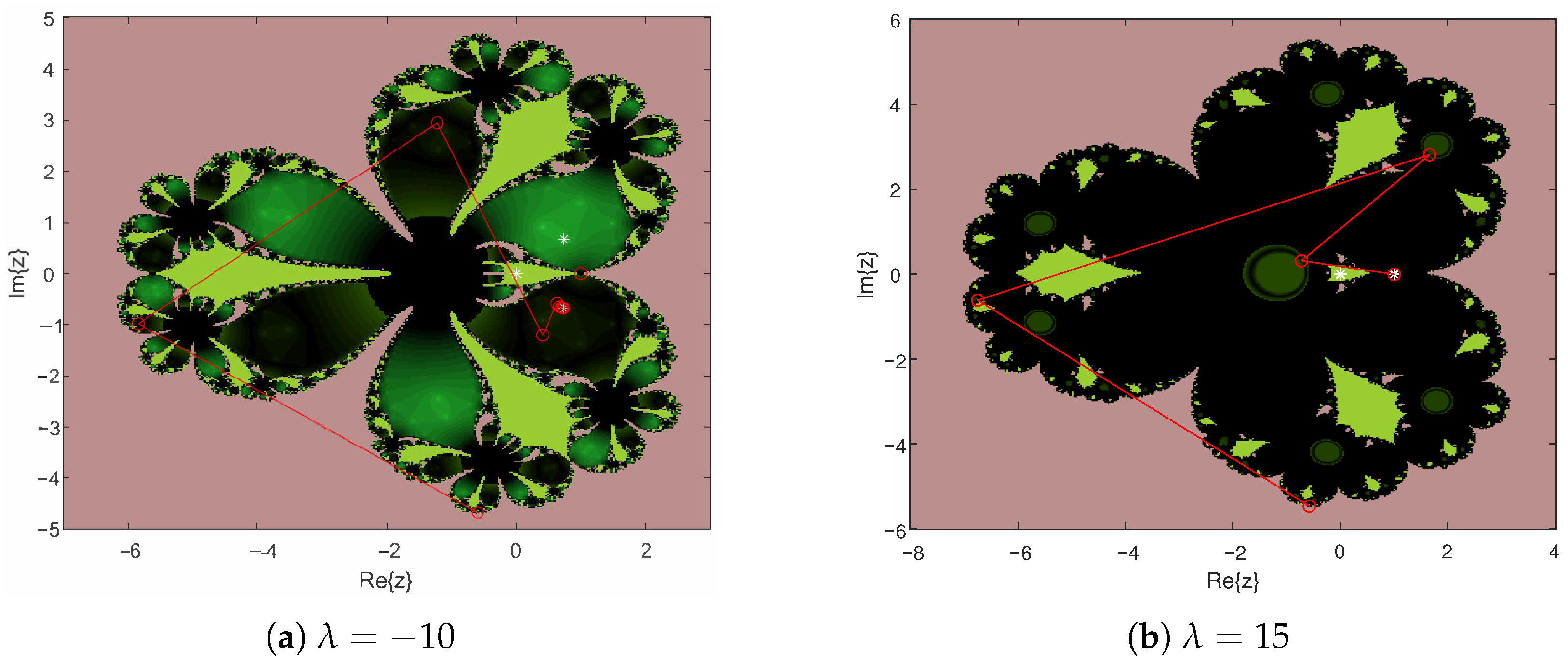
In this part, some representative parameter values are selected to plot the corresponding dynamic plane. The dynamic plane drawn in this paper uses $400\times 400$ grid points, and the maximum number of iterations is set to 25. Different colors represent convergence to different roots; fleshly pink represents convergence to infinity, grassy green represents convergence to 0, dark green represents convergence to $x=1$, and finally black areas represent non-convergence or divergence. The asterisks in the Figure 5, Figure 6, Figure 7 and Figure 8 denoted the fixed points. In the parameter plane above, we know that the convergence effect is better when the parameter values are taken in the green and blue regions, and the effect is not ideal when the parameter values are in the orange region. Therefore, we obtain parameter values in the blue, green, and orange regions, respectively, to plot the relevant dynamic planes and observe their effects.

Figure 5. Dynamic plane of stable parameter values.

Figure 6. Dynamic planes of special $\lambda$.

Figure 7. The dynamic plane of $x=1$ is a saddle point.

Figure 8. Dynamic plane of unstable parameter values.

In Figure 5, we selected some of the special parameter values mentioned above to draw the dynamic plane, where when $\lambda =-{\displaystyle \frac{25}{54}}$, $\lambda =-{\displaystyle \frac{1}{2}}$ and $\lambda =0$, the convergence effect of the iterative method is better. And at $\lambda ={\displaystyle \frac{5}{2}}$, there are some black areas in the diagram that do not converge or diverge. We obtained some parameter values in the green and blue areas of the parameter planes to draw the corresponding dynamic planes, as shown in Figure 6, and obtained some stable images. Figure 7 shows the parameter values when $x=1$ is a saddle point. In these case, a large black region and any region converging to $x=1$ appear in the correlated dynamic planes, which are not ideal results. The parameter values in Figure 8 are selected in the orange region of the parameter planes, and the resulting dynamic planes still present complex situations. Finally, the parameter values take points around 0, which has a good convergence effect.

5. Comparison of Fractal Diagrams for Different Methods

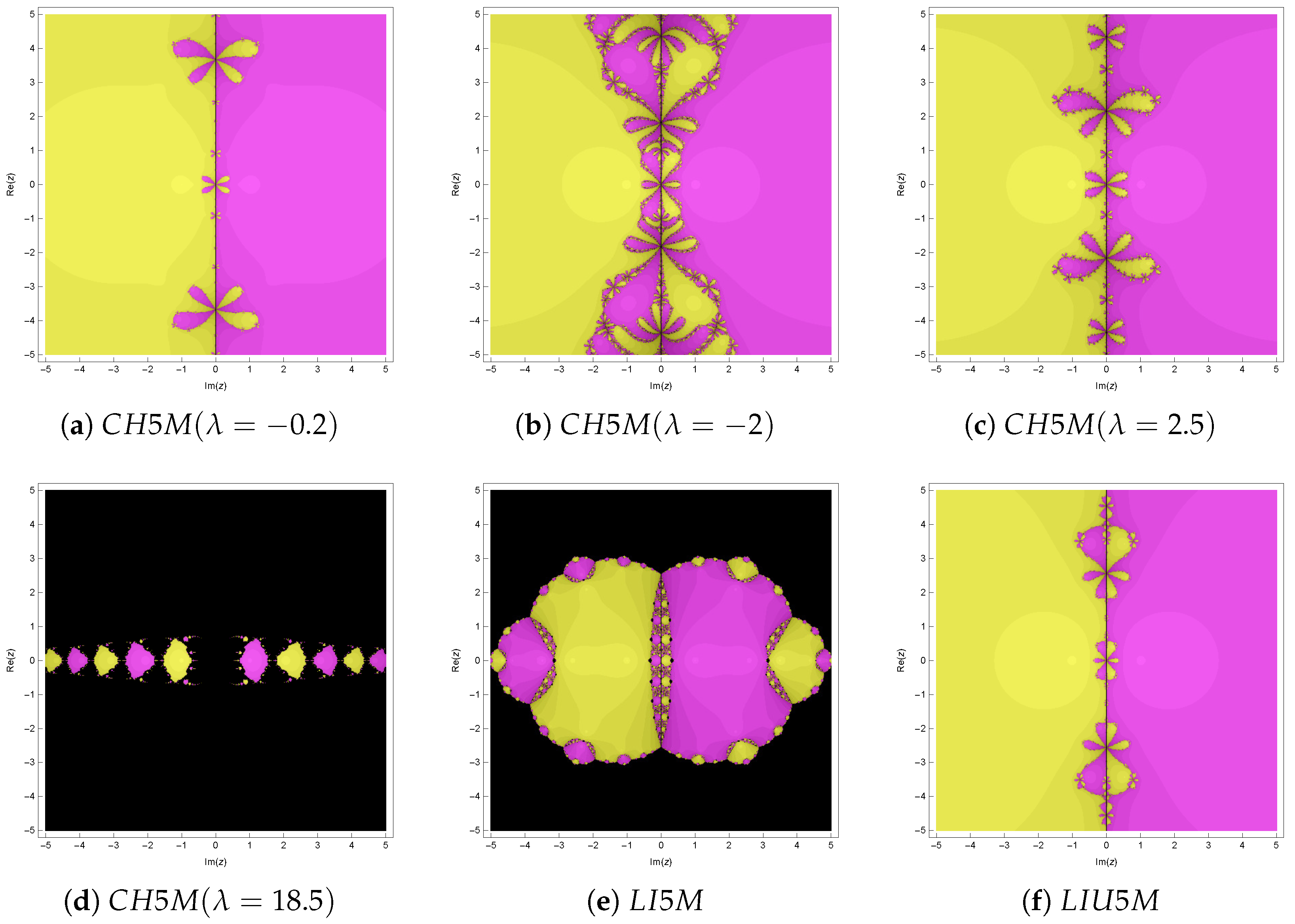
In this section, the fractal diagrams of the new method about polynomials $G\left(x\right)=x^2-1$ are compared with method LI5M [32] and method LIU5M [33]. Method LI5M [32] is

$$\left\{\begin{array}{c}{y}_n=x_n-{\displaystyle \frac{f\left(x_n\right)}{f^{\prime }\left(x_n\right)}},\\ z_n=y_n-{\displaystyle \frac{f\left(y_n\right)}{f\left(x_n\right)-4f\left(y_n\right)}}{\displaystyle \frac{f\left(x_n\right)}{f^{\prime }\left(x_n\right)}},\\ x_{n+1}=z_n-{\displaystyle \frac{f\left(z_n\right)}{f^{\prime }\left(x_n\right)+\frac{2f\left(y_n\right)f^{\prime }{\left(x_n\right)}^2}{f{\left(x_n\right)}^2}(z_n-x_n)}},\end{array}\right.$$

(43)

Method LIU5M [33] is

$$\left\{\begin{array}{c}{y}_n=x_n-{\displaystyle \frac{f\left(x_n\right)}{f^{\prime }\left(x_n\right)}},\\ \\ x_{n+1}=y_n-{\displaystyle \frac{f\left(y_n\right)}{f^{\prime }\left(y_n\right)}}-{\displaystyle \frac{{f\left(y_n\right)}^2{f}^{\prime \prime }\left(y_n\right)}{2{f^{\prime }\left(x_n\right)}^2{f}^{\prime }\left(y_n\right)}}.\end{array}\right.$$

(44)

In this article, we chose $500\times 500$ points and set the maximum number of iterations to 25. Different colors represent convergence to different roots, and the black area indicates that divergence or reaching the maximum number of iterations does not converge. In Figure 9, several stable and unstable parameters are selected to draw a fractal graph corresponding to the iterative method on $x^2-1$. The graph in method CH5M ($\lambda =-0.2$) is simple and has fewer black areas than other methods. Therefore, the stability and convergence of this iterative method are better than other methods.

Figure 9. Fractal diagrams of the methods about polynomials $x^2-1$.

6. Numerical Results

In this part, we conduct the corresponding numerical experiments according to the above work. First, the properties of the iterative method depend on the values of the parameters. Therefore, the numerical results of the iterative methods corresponding to different parameter values are compared. Next, the numerical results of the new iterative method are compared with those of other different fifth-order iterative methods.

Table 1, Table 2 and Table 3 show the following information: ACOC is the approximated computational order of convergence, $|x_k-x_{k-1}|$ is the absolute error, EI is the computational efficiency index, and Time refers to the CPU time (in seconds). We compared the computation time and precision of the iterative method under four iterations. The data precision is set to 2400 digits. The approximate computational order of convergence (ACOC) [34] is computed using the formula

$$ACOC={\displaystyle \frac{ln\left(\right|x_{k+1}-x_k|/|x_k-x_{k-1}\left|\right)}{ln\left(\right|x_k-x_{k-1}|/|x_{k-1}-x_{k-2}\left|\right)}},$$

Table 1. Numerical results for stable parameter values.

${\mathit{f}}_{\mathit{i}}\left(\mathit{x}\right)$	$\mathit{\lambda }$	${\mathit{x}}_0$	$|{\mathit{x}}_1-{\mathit{x}}_0|$	$|{\mathit{x}}_2-{\mathit{x}}_1|$	$|{\mathit{x}}_3-{\mathit{x}}_2|$	$|{\mathit{x}}_4-{\mathit{x}}_3|$	EI	ACOC
$f_1\left(x\right)$	0	2.1	0.054435	1.041 × 10−8	1.8915 × 10−42	3.746 × 10−211	1.495	5.0
	−0.1	2.1	0.054435	4.3176 × 10−10	4.643 × 10−50	6.6767 × 10−250	1.495	5.0
	$-{\displaystyle \frac{1}{2}}$	2.1	0.054435	4.1688 × 10−8	9.7406 × 10−39	6.7832 × 10−192	1.495	5.0
	0	2.2	0.045565	2.1689 × 10−9	7.4262 × 10−46	3.4944 × 10−228	1.495	5.0
	−0.1	2.2	0.045565	1.1265 × 10−9	5.6142 × 10−48	1.7258 × 10−239	1.495	5.0
	$-{\displaystyle \frac{1}{2}}$	2.2	0.045565	1.3786 × 10−8	3.8515 × 10−41	6.5567 × 10−204	1.495	5.0
$f_2\left(x\right)$	0	1.3	0.06523	2.2322 × 10−8	6.0964 × 10−41	9.2642 × 10−204	1.495	5.0
	−0.1	1.3	0.06523	2.0084 × 10−9	2.1124 × 10−46	2.719 × 10−231	1.495	5.0
	$-{\displaystyle \frac{1}{2}}$	1.3	0.06523	1.0889 × 10−7	1.1683 × 10−36	1.6615 × 10−181	1.495	5.0
	0	1.4	0.04247	5.1534 × 10−10	9.5535 × 10−50	2.0917 × 10−248	1.495	5.0
	−0.1	1.4	0.03477	4.2257 × 10−10	8.7093 × 10−50	3.2391 × 10−248	1.495	5.0
	$-{\displaystyle \frac{1}{2}}$	1.4	0.03477	3.523 × 10−9	4.1422 × 10−44	9.3071 × 10−219	1.495	5.0
$f_3\left(x\right)$	0	1.5	0.025994	9.2855 × 10−9	4.0688 × 10−41	6.5737 × 10−203	1.495	5.0
	−0.1	1.5	0.025994	1.6364 × 10−9	8.368 × 10−47	2.9262 × 10−233	1.495	5.0
	$-{\displaystyle \frac{1}{2}}$	1.5	0.025994	3.0454 × 10−8	6.0831 × 10−38	1.9343 × 10−186	1.495	5.0
	0	1.6	0.074006	4.1994 × 10−7	7.6987 × 10−33	1.5942 × 10−161	1.495	5.0
	−0.1	1.6	0.074007	5.3893 × 10−7	3.2434 × 10−34	2.5599 × 10−170	1.495	5.0
	$-{\displaystyle \frac{1}{2}}$	1.6	0.07401	3.9657 × 10−6	2.2776 × 10−27	1.4233 × 10−133	1.495	5.0
$f_4\left(x\right)$	0	1.4	0.0044916	5.1534 × 10−10	9.5535 × 10−50	2.0917 × 10−248	1.495	5.0
	−0.1	1.4	0.0044916	7.38 × 10−14	9.0937 × 10−68	2.5832 × 10−337	1.495	5.0
	$-{\displaystyle \frac{1}{2}}$	1.4	0.0044916	4.9068 × 10−14	6.5608 × 10−69	2.8039 × 10−343	1.495	5.0
	0	1.5	0.04247	5.1534 × 10−10	9.5535 × 10−50	2.0917 × 10−248	1.495	5.0
	−0.1	1.5	0.095509	2.9334 × 10−7	9.0214 × 10−35	2.4821 × 10−172	1.495	5.0
	$-{\displaystyle \frac{1}{2}}$	1.5	0.095508	1.2215 × 10−7	6.2732 × 10−37	2.2408 × 10−183	1.495	5.0
$f_5\left(x\right)$	0	−0.4	0.042854	3.2432 × 10−8	9.4964 × 10−39	2.0441 × 10−191	1.495	5.0
	−0.1	−0.4	0.042854	8.7359 × 10−9	4.693 × 10−42	2.0998 × 10−208	1.495	5.0
	$-{\displaystyle \frac{1}{2}}$	−0.4	0.042854	8.3083 × 10−8	2.3652 × 10−36	4.4222 × 10−179	1.495	5.0
	0	−0.5	0.057145	1.9746 × 10−7	7.9457 × 10−35	8.3822 × 10−172	1.495	5.0
	−0.1	−0.5	0.057146	8.5069 × 10−8	4.1094 × 10−37	1.081 × 10−183	1.495	5.0
	$-{\displaystyle \frac{1}{2}}$	−0.5	0.057146	3.8502 × 10−7	5.0553 × 10−33	1.9727 × 10−162	1.495	5.0

Table 2. Numerical results of different iterative methods.

${\mathit{f}}_{\mathit{i}}\left(\mathit{x}\right)$	Methed	${\mathit{x}}_0$	$|{\mathit{x}}_1-{\mathit{x}}_0|$	$|{\mathit{x}}_2-{\mathit{x}}_1|$	$|{\mathit{x}}_3-{\mathit{x}}_2|$	$|{\mathit{x}}_4-{\mathit{x}}_3|$	EI	Time	ACOC
$f_1\left(x\right)$	CH5M	2.1	0.054435	9.7672 × 10−9	1.9254 × 10−42	5.7317 × 10−211	1.495	0.859375	5.0
	LI5M	2.1	0.054435	1.1860 × 10−8	7.2608 × 10−42	6.2445 × 10−208	1.495	0.984375	5.0
	LIU5M	2.1	0.054435	1.0285 × 10−7	2.1370 × 10−36	8.2752 × 10−180	1.380	0.953125	5.0
	CH5M	2.2	0.045565	4.3697 × 10−9	3.4509 × 10−44	1.06 × 10−219	1.495	0.859375	5.0
	LI5M	2.2	0.045565	7.1280 × 10−9	5.6938 × 10−43	1.8518 × 10−213	1.495	0.953125	5.0
	LIU5M	2.2	0.045565	3.2342 × 10−8	6.5699 × 10−39	2.2725 × 10−192	1.380	0.875000	5.0
$f_2\left(x\right)$	CH5M	1.3	0.06523	2.7294 × 10−8	3.6249 × 10−40	1.4976 × 10−199	1.495	1	5.0
	LI5M	1.3	0.06523	2.3825 × 10−8	2.2347 × 10−40	1.6224 × 10−200	1.495	1.06250	5.0
	LIU5M	1.3	0.06523	3.3406 × 10−7	9.6132 × 10−34	1.897 × 10−166	1.380	1.062500	5.0
	CH5M	1.4	0.03477	1.2182 × 10−9	6.4193 × 10−47	2.6083 × 10−233	1.495	0.96875	5.0
	LI5M	1.4	0.03477	1.7212 × 10−9	4.3970 × 10−46	4.7842 × 10−229	1.495	1.078125	5.0
	LIU5M	1.4	0.03477	1.7212 × 10−9	3.0664 × 10−41	6.2639 × 10−204	1.380	1.015625	5.0
$f_3\left(x\right)$	CH5M	1.5	0.025994	6.1621 × 10−9	5.1104 × 10−42	2.005 × 10−207	1.495	2.15625	5.0
	LI5M	1.5	0.025994	9.2354 × 10−9	6.5207 × 10−41	1.1442 × 10−201	1.495	2.84375	5.0
	LIU5M	1.5	0.025994	6.6011 × 10−8	6.0088 × 10−36	3.7554 × 10−176	1.380	2.421875	5.0
	CH5M	1.6	0.074008	1.4569 × 10−6	3.7752 × 10−30	4.4111 × 10−148	1.495	2.218750	5.0
	LI5M	1.6	0.074002	3.6376 × 10−6	6.1819 × 10−28	8.7625 × 10−137	1.495	3	5.0
	LIU5M	1.6	0.073999	7.1484 × 10−6	8.9483 × 10−26	2.7505 × 10−125	1.380	2.328125	5.0
$f_4\left(x\right)$	CH5M	1.4	0.0044916	1.9748 × 10−13	3.1876 × 10−65	3.4933 × 10−324	1.495	5.78125	5.0
	LI5M	1.4	0.0044916	1.8885 × 10−13	2.5866 × 10−65	1.2466 × 10−324	1.495	5.9375	5.0
	LIU5M	1.4	0.0044916	2.8232 × 10−12	2.7044 × 10−58	2.1813 × 10−288	1.380	9.09375	5.0
	CH5M	1.5	0.095509	4.3341 × 10−7	1.6232 × 10−33	1.196 × 10−165	1.495	5.53125	5.0
	LI5M	1.5	0.095507	0.14697 × 10−6	7.3846 × 10−31	2.3645 × 10−152	1.495	5.96875	5.0
	LIU5M	1.5	0.095501	7.3653 × 10−6	3.2682 × 10−26	5.6221 × 10−128	1.380	8.953125	5.0
$f_5\left(x\right)$	CH5M	−0.4	0.042854	1.4664 × 10−8	5.4363 × 10−41	3.8072 × 10−203	1.495	2.234375	5.0
	LI5M	−0.4	0.042854	5.1687 × 10−8	1.0601 × 10−37	3.8484 × 10−186	1.495	2.734375	5.0
	LIU5M	−0.4	0.042854	1.1932 × 10−7	2.2641 × 10−35	5.5691 × 10−174	1.380	2.296875	5.0
	CH5M	−0.5	0.057146	2.9376 × 10−8	1.7542 × 10−39	1.332 × 10−195	1.495	2.265625	5.0
	LI5M	−0.5	0.057145	1.2954 × 10−7	1.0481 × 10−35	3.6347 × 10−176	1.495	2.703125	5.0
	LIU5M	−0.5	0.057145	6.7844 × 10−7	1.3455 × 10−31	4.1285 × 10−155	1.380	2.328125	5.0

Table 3. Numerical results of different iterative methods for the Van der Waals Equation (32).

Methed	${\mathit{x}}_0$	$|{\mathit{x}}_1-{\mathit{x}}_0|$	$|{\mathit{x}}_2-{\mathit{x}}_1|$	$|{\mathit{x}}_3-{\mathit{x}}_2|$	$|{\mathit{x}}_4-{\mathit{x}}_3|$	EI	Time	ACOC
CH5M	2	0.29216 × 10−1	0.13939 × 10−7	0.34584 × 10−39	0.32520 × 10−197	1.495	1.109375	5.0
LI5M	2	0.29216 × 10−1	0.22409 × 10−7	0.45219 × 10−38	0.15130 × 10−191	1.495	1.218750	5.0
LIU5M	2	0.29216 × 10−1	0.11075 × 10−6	0.10565 × 10−33	0.83462 × 10−169	1.380	1.125000	5.0
CH5M	2.3	0.33057	0.33057	0.30071 × 10−14	0.16162 × 10−72	1.495	1.109375	5.0
LI5M	2.3	0.29840	0.30819 × 10−1	0.29663 × 10−7	0.18378 × 10−37	1.495	1.265625	5.0
LIU5M	2.3	0.32531	0.39098 × 10−2	0.56386 × 10−11	0.36141 × 10−55	1.380	1.203125	5.0

And the computational efficiency index (EI) [31] is computed by

$$EI=r^{1/n},$$

where r is the convergence order and n is the number of functional evaluations.

First experiment: In this experiment we use the following equations

$$f_1\left(x\right)=x^3-10,\alpha \approx 2.1544346900318837$$

$$f_2\left(x\right)=x^3+4x^2-10,\alpha \approx 1.3652300134140968$$

$$f_3\left(x\right)=x^4-lg\left(x\right)-5,\alpha \approx 1.5259939537536892$$

$$f_4\left(x\right)=si{n}^{2}x-x^2+1,\alpha \approx 1.4044916482153412$$

$$f_5\left(x\right)=(x+2)e^x-1,\alpha \approx -0.44285440100238858$$

Second experiment: The well-known Van der Waals equation [35] is represented as follows:

$$p+{\displaystyle \frac{n^{2}k}{v^2}}(V-nh)=nRT$$

where k and h are positive constants. Constants $P,V,T$ are the pressure, volume, and temperature of gas. The equation can be simplified as follows:

$$f\left(V\right)=n^{2}kV+hPn-TR{V}^2+P{V}^3-hk{n}^3$$

Taking $k=18,P=40,n=1.4,h=0.1154,$ and $T=500$, we can obtain the following polynomial:

$$f\left(V\right)=35.28V-95.26535V^2-5.6998363+40V^3.$$

(45)

Table 1 presents a comparison of the numerical results for the iterative methods corresponding to different parameter values, namely, $\lambda =0,\lambda =-0.1$, and $\lambda =-{\displaystyle \frac{1}{2}}$. Among these, the iterative method with $\lambda =-0.1$ exhibits the optimal convergence performance and the highest computational accuracy. Table 2 and Table 3 compare the numerical results of the proposed method (CH5M) with those of the LI5M and LIU5M methods when the parameter is set to $-0.2$. The computational accuracy of CH5M is significantly superior to that of the other two methods, and its computation time is also shorter. Notably, CH5M and LI5M achieve equivalent computational efficiency, both of which outperform LIU5M.

7. Conclusions

In this paper, a class of fifth-order parametric Chebyshev–Halley-type iterative methods is proposed. Compared with the classical third-order Chebyshev–Halley method, the proposed method achieves fifth-order convergence accuracy with only one additional function evaluation. Our method has the same convergence order and computational cost with the existing Chebyshev–Halley-type families. The difference lies in that our method uses one first-order derivative, one second-order derivative, and two function values, while other methods use one first-order derivative and three function values. The classic Chebyshev–Halley method incorporates the second-order derivative in its iterative formula. To retain this characteristic, our new method still includes the second-order derivative in its iterative format. The convergence of the new method is proved via Taylor expansion, and a systematic analysis of its dynamic characteristics is carried out as follows: the fixed points and critical points of the relevant iterative operators are solved, and the stability of the fixed points is determined. To screen the family members with stable convergence effects, these critical points are used as initial iteration points to plot the parameter planes and the corresponding dynamic planes, which intuitively present the stability distribution characteristics of the iterative method. The analysis results show that when the parameter takes values near 0 (e.g., $\lambda =-{\displaystyle \frac{25}{54}},\lambda =-{\displaystyle \frac{1}{2}},\lambda =-{\displaystyle \frac{1}{10}},\lambda =0$, and $\lambda =1$.), the method exhibits excellent stability and convergence performance. Relevant fractal graphs and numerical experiment results further verify this conclusion.

References

1. Mandelbrot, B.B.; Aizenman, M. Fractals: Form, Chance, and Dimension. Phys. Today 1979, 32, 65–66. [Google Scholar] [CrossRef]
2. Hirano, M.; Nagahama, H. Informative fractal dimension associated with nonmetricity in information geometry. Phys. A 2023, 625, 129017. [Google Scholar] [CrossRef]
3. Qiang, C.; Deng, Y.; Cheong, K.H. Information fractal dimension of mass function. Fractals 2022, 30, 2250110. [Google Scholar] [CrossRef]
4. Chen, X.; Li, T.; Shen, J.; Hu, Z. Fractal design of microfluidics and nanofluidics—A review. Chemometr. Intell. Lab. Syst. 2016, 155, 19–25. [Google Scholar] [CrossRef]
5. Sala, N. Fractal geometry in the arts: An overview across the different cultures. Pattern Recognit. 2004, 177–188. [Google Scholar]
6. Peitgen, H.; Richter, P. The Beauty of Fractals; Springer: New York, NY, USA, 1986. [Google Scholar]
7. Bock, H. On the dynamics of entire functions on the Julia set. Results Math. 1996, 30, 16–20. [Google Scholar] [CrossRef]
8. Letherman, S.D.; Wood, R.M.W. A note on the Julia set of a rational function. Math. Proc. Camb. Philos. Soc. 1995, 118, 477–485. [Google Scholar] [CrossRef]
9. Hua, X.; Yang, C.C. Fatou Components and a Problem of Bergweiler. Int. J. Bifurc. Chaos Appl. Sci. Eng. 1998, 8, 1613–1616. [Google Scholar] [CrossRef]
10. Cordero, A.; Jaiswal, J.P.; Torregrosa, J.R. Stability analysis of fourth-order iterative method for finding multiple roots of non-linear equations. Appl. Math. Nonlinear Sci. 2019, 4, 43–56. [Google Scholar] [CrossRef]
11. Behl, R.; Cordero, A.; Motsa, S.S.; Torregrosa, J.R. On optimal fourth-order optimal families of methods for multiple roots and their dynamics. Appl. Math. Comput. 2015, 265, 520–532. [Google Scholar]
12. Guo, Y.; Wu, Q.; Wang, X. An extension of high-order Kou’s method for solving nonlinear systems and its stability analysis. Electron. Res. Arch. 2025, 33, 1566–1588. [Google Scholar] [CrossRef]
13. Yu, J.; Wang, X.F. A single parameter fourth-order Jarrat-type iterative method for solving nonlinear systems. AIMS Math. 2025, 10, 7847–7863. [Google Scholar] [CrossRef]
14. Lee, M.Y.; Kim, Y.I. The dynamical analysis of a uniparametric family of three-point optimal eighth-order multiple-root finders under the Möbius conjugacy map on the Riemann sphere. Numer. Algorithms 2020, 83, 1063–1090. [Google Scholar] [CrossRef]
15. Chicharro, F.I.; Cordero, A.; Torregrosa, J.R. Drawing dynamical and parameters planes of iterative families and methods. Sci. World J. 2013, 2013, 780153. [Google Scholar] [CrossRef] [PubMed]
16. Wang, X.F.; Li, W.S. Fractal behavior of king’s optimal eighth-order iterative method and its numerical application. Math. Commun. 2024, 29, 217–236. [Google Scholar]
17. Capdevila, R.R.; Cordero, A.; Torregrosa, J.R. Isonormal surfaces: A new tool for the multi-dimensional dynamical analysis of iterative methods for solving nonlinear systems. Math. Meth. Appl. Sci. 2022, 45, 3375. [Google Scholar] [CrossRef]
18. Campos, B.; Cordero, A.; Torregrosa, J.R.; Vindel, P. Dynamical analysis of an iterative method with memory on a family of third-degree polynomials. AIMS Math. 2022, 7, 6445–6466. [Google Scholar] [CrossRef]
19. Cordero, A.; Segura, E.; Torregrosa, J.R.; Vassileva, M.P. Inverse matrix estimations by iterative methods with weight functions and their stability analysis. Appl. Math. Lett. 2024, 155, 109122. [Google Scholar] [CrossRef]
20. Chicharro, F.I.; Cordero, A.; Garrido, N.; Torregrosa, J.R. On the effect of the multidimensional weight functions on the stability of iterative processes. J. Comput. Appl. Math. 2022, 405, 113052. [Google Scholar] [CrossRef]
21. Moscoso-Martínez, M.; Chicharro, F.I.; Cordero, A.; Torregrosa, J.R.; Ureña-Callay, G. Achieving Optimal Order in a Novel Family of Numerical Methods: Insights from Convergence and Dynamical Analysis Results. Axioms 2024, 13, 458. [Google Scholar] [CrossRef]
22. Wang, X.; Zhang, T. Efficient n-point iterative methods with memory for solving nonlinear equations. Numer. Algorithms 2015, 70, 357–375. [Google Scholar] [CrossRef]
23. Jarratt, P. Some fourth order multipoint iterative methods for solving equations. Math. Comput. 1966, 20, 434–437. [Google Scholar] [CrossRef]
24. Ostrowski, A.M. Solution of Equations in Euclidean and Banach Spaces; Academic Press: New York, NY, USA, 1973. [Google Scholar]
25. Shang, N.; Wang, X.F.; Wang, Y. Local convergence analysis of a novel Kurchatov-type derivative-free methods with and without memory for solving nonlinear systems. Int. J. Comput. Methods 2026, 23, 2550033. [Google Scholar] [CrossRef]
26. Wang, X. An Ostrowski-type method with memory using a novel self-accelerating parameter. J. Comput. Appl. Math. 2018, 330, 710–720. [Google Scholar] [CrossRef]
27. Candela, V.; Marquina, A. Recurrence relations for rational cubic methods II: The Chebyshev method. Computing 1991, 45, 355–367. [Google Scholar] [CrossRef]
28. Alefeld, G. On the convergence of Halley’s Method. Am. Math. Mon. 1981, 88, 530–536. [Google Scholar] [CrossRef]
29. Chen, D.; Argyros, I.K.; Qian, Q. A local convergence theorem for the super-Halley method in a Banach space. Appl. Math. Lett. 1994, 7, 49–52. [Google Scholar] [CrossRef]
30. Gutierrez, J.M.; Hernández, M.A. A family of Chebyshev-Halley type methods in Banach spaces. Bull. Aust. Math. Soc. 1997, 55, 113–130. [Google Scholar] [CrossRef]
31. Ostrowski, A.M. Solution of Equation and Systems of Equations; Academic Press: New York, NY, USA, 1960. [Google Scholar]
32. Li, D.; Liu, P.; Kou, J. An improvement of Chebyshev–Halley methods free from second derivative. Appl. Math. Comput. 2014, 235, 221–225. [Google Scholar] [CrossRef]
33. Rafiullah, M. A fifth-order iterative method for solving nonlinear equations. Numer. Anal. Appl. 2021, 4, 239–243. [Google Scholar] [CrossRef]
34. Cordero, A.; Gomez, E.; Torregrosa, J.R. Efficient high-order iterative methods for solving nonlinear systems and their application on heat conduction problems. Complexity 2017, 2017, 6457532. [Google Scholar] [CrossRef]
35. Chang, C.W.; Qureshi, S.; Argyros, I.K.; Chicharro, F.I.; Soomro, A. A modified two-step optimal iterative method for solving nonlinear models in one and higher dimensions. Math. Comput. Simul. 2025, 229, 448–467. [Google Scholar] [CrossRef]