Article

A Physics-Informed Neural Network Based on the Separation of Variables for Solving the Distributed-Order Time-Fractional Advection–Diffusion Equation

School of Mathematical Sciences, Inner Mongolia University, Hohhot 010021, China
*
Author to whom correspondence should be addressed.
Fractal Fract. 2025, 9(11), 712; https://doi.org/10.3390/fractalfract9110712
Submission received: 19 September 2025 / Revised: 24 October 2025 / Accepted: 31 October 2025 / Published: 4 November 2025

Abstract

In this work, we propose a new physics-informed neural network framework based on the method of separation of variables (SVPINN) to solve the distributed-order time-fractional advection–diffusion equation. We develop a new method for calculating the distributed-order derivative, which enables the fractional integral to be modeled by a network and directly solved by combining automatic differentiation technology. In this way, the approximation of the distributed-order derivative is integrated into the parameter training system of the network, and the data-driven adaptive learning mechanism is used to replace the numerical discretization scheme. In the SVPINN framework, we decompose the kernel function of the Caputo integral into three independent functions using the method of separation of variables, and apply a neural network as a surrogate model for the modified integral and the function related to the time variable. The new physical constraint generated by the modified integral serves as an extra supervised learning task for the network. We systematically evaluated the feasibility of the SVPINN on several numerical experiments and demonstrated its performance.

1. Introduction

In the fields of science and engineering, efficient modeling and solving of complex physical systems have always been a core challenge. Traditional numerical methods, such as the finite element method and the finite difference method, face bottlenecks such as high computational costs and weak model generalization ability when dealing with high-dimensional problems and complex boundary conditions. In recent years, with the rapid development of machine learning, especially the breakthroughs in function approximation and data-driven modeling in deep learning, physics-informed neural network (PINN) [1] that combines physical prior knowledge with a neural network has emerged, providing a new paradigm for solving the above problems.
Since the PINN framework was proposed, it has made breakthrough progress in fields such as fluid mechanics [2,3,4,5], solid mechanics [6,7,8], heat conduction [9,10], and materials science [11]. To enhance the performance of the PINN, researchers have proposed a series of advanced optimization methods based on the model and problem characteristics. From the perspective of the PINN model, the main ways to improve the generalization ability and training efficiency of the model are through adjusting the network structure [12,13,14,15,16], introducing attention mechanism [17] or adaptive idea [18], optimizing the construction of loss functions [19,20,21,22], and making improvements to training strategies [23,24,25]. Starting from the perspective of problem characteristics, domain decomposition techniques are adopted to refine the problem-solving space [26,27], and additional constraint conditions are introduced to further optimize the model [28,29,30], thereby achieving a comprehensive improvement in overall performance.
However, despite the enormous potential demonstrated by the PINN, it fails to directly solve fractional partial differential equations (FPDEs) due to the inability of the automatic differentiation technique to calculate integrals. Pang et al. [31] proposed using the finite difference method, the Grünwald–Letnikov scheme, to approximate fractional derivatives and developed fractional PINNs (fPINNs). Ma et al. [32] used the L1 formula and the L2 1 σ formula to approximate Caputo derivatives. Sivalingam et al. [33] applied the theory of functional connection to solve Caputo-type problems. Guo et al. [34] used a Monte Carlo strategy to approximate fractional derivatives. Subsequent studies continue to use different numerical schemes to solve FPDEs [35,36,37].
The advection–diffusion equation can effectively characterize transport processes in both engineering and natural phenomena. However, the description of transport processes in various physical or biological systems often exhibits anomalous diffusion behavior. For instance, particle propagation speed deviates from Fick’s law, and the growth rate of mean square displacement shows a nonlinear relationship with time. These phenomena also occur in other transportation scenarios, such as pollutant migration, groundwater flow, and turbulent transport. The fractional advection–diffusion equation can more accurately describe these complex dynamic processes. The fractional derivative utilizes a memory kernel in the form of a power function to weight the entire historical process, which gives the model a memory effect and significantly improves its ability to model and predict transport behavior in complex systems, attracting widespread attention.
As a significant extension of fractional derivatives, distributed-order derivatives break through the limitation of fixed-order derivatives and expand the derivative order from a single numerical value to a continuous interval description based on distributed functions. Although this feature enhances the ability of equations to describe complex physical processes, it also increases the difficulty of solving them. To address this challenge, some scholars have drawn on the discretization idea of fractional derivatives in fPINN. In the recently proposed PINN-based framework, Ramezani et al. [38] used composite midpoint and L1 formulae to approximate the distributed-order derivative, while Momeni et al. [39] combined the Legendre–Gauss quadrature rule and operational matrices to discretize the distributed-order derivative. Other scholars also use numerical schemes to convert the distributed-order derivatives into a processable form, and then embed them into a neural network [40,41,42,43].
However, there are two issues with this approach: (1) PINN-based frameworks rely on numerical schemes such as finite difference to discretize the distributed-order derivative; (2) the approximation of the distributed-order derivative cannot be achieved by optimizing the parameters of the network. Therefore, the accuracy of the solution is limited by the precision of the numerical discretization method, rather than the approximation ability of the network. These issues drive the primary objective of this work.
In this paper, we present a new framework based on the PINN, called SVPINN, to solve the distributed-order time-fractional advection–diffusion equation. The proposed method changes the integral form by separating variables, which allows the neural network to directly approximate the distributed-order derivative. The main contributions of this paper are as follows: (1) We propose a variable separation-based PINN framework suitable for the distributed-order derivative. Unlike the classical separation of variables method that seeks analytical solutions, a neural network is utilized to approximate the variable-based basis functions to achieve the variable separation process, as the kernel function in the Caputo derivative is not strictly separable. (2) The proposed SVPINN decomposes the kernel function in the Caputo derivative into the product form of basis functions consisting of time variable, integral variable, and order. This avoids using a numerical discretization scheme to approximate the distributed-order derivative, thereby eliminating integral discretization. (3) In the SVPINN framework, the approximation of the distributed-order derivative is gradually completed by training the parameters of the network during the training process, which is different from the PINN-based frameworks proposed in [40,41,42,43] that directly complete the approximation of the distributed-order derivative using a numerical scheme before the training process. (4) Compared with the PINN that simulates the fractional derivative using numerical discretization scheme, the SVPINN significantly improves prediction accuracy and convergence speed in irregular domains and high-dimensional problems.
The structure of this paper is as follows: In Section 2, the detailed framework of the SVPINN is presented. In Section 3, several numerical examples are used to test the performance of our proposed method. In Section 4, we summarize several concluding remarks.

2. Method

In this section, we first clarify the distributed-order advection–diffusion equation and the definition of the distributed-order derivative. Then we present a detailed introduction to the structure of our proposed method. Finally, we analyze the stability of the proposed SVPINN.

2.1. Problem Setup

In this study, we focus on the following distributed-order time-fractional advection–diffusion equation
D t ω ( α ) u Δ u + R · u = h ( x , t ) , ( x , t ) Ω × τ ,
with the boundary condition
u ( x , t ) = B ( x , t ) , ( x , t ) Ω ¯ × τ ¯ ,
and the initial condition
u ( x , 0 ) = I ( x ) , x Ω ¯ ,
where R = ( 1 , 1 , , 1 ) R d denotes a constant advection velocity. Also D t ω ( α ) represents the distributed-order derivative, having
D t ω ( α ) u ( x , t ) = 0 1 ω ( α ) 0 C D t α u ( x , t ) d α ,
with the Caputo fractional derivative [40,41,42,43]
D t α a C u ( x , t ) = 1 Γ ( 1 α ) a t ( t η ) α u η ( x , η ) d η , 0 α < 1 , α u ( x , t ) t α , α = 1 ,
where ( t η ) α represents the kernel function, ω ( α ) > 0 , and 0 < 0 1 ω ( α ) d α < . In the framework of the distributed-order derivative, the order α varies as an integral variable, rather than remaining fixed. The influence of any individual order α is determined by the weight function ω ( α ) .

2.2. The SVPINN Framework

Based on the integral (4), without considering other variables such as the space variable x and the time variable t, we can simply regard the integral as
0 1 ω ( α ) D t α 0 C u ( x , t ) d α = 0 1 ω ( α ) A ( α ) d α ,
where the function A ( α ) is only related to the integral variable α . Similarly, for the integral in (5), if we can separate t and η in the kernel function ( t η ) α , then we have
a t ( t η ) α u η ( x , η ) d η = T ( t ) a t N ( η ) u η ( x , η ) d η ,
where T ( t ) and N ( η ) are only related to variables t and n, respectively. On the basis of the above conjecture, we plan to construct a new integral form of the distributed-order derivative by separating variables.
For the kernel function ( t η ) α , we apply the method of separation of variables to decompose it into the following form
( t η ) α T ( t ) N ( η ) A ( α ) .
Then, the Caputo fractional derivative can be rewritten as
D t α a C u ( x , t ) 1 Γ ( 1 α ) A ( α ) T ( t ) a t N ( η ) u η ( x , η ) d η .
For the distributed-order derivative D t ω ( α ) u ( x , t ) , we have
0 1 ω ( α ) D t α 0 C u ( x , t ) d α D ( x , t , u ) 0 1 ω ( α ) Γ ( 1 α ) A ( α ) d α ,
where
D ( x , t , u ) = T ( t ) a t N ( η ) u η ( x , η ) d η .
Given that ψ ( x , t ) = a t N ( η ) u η ( x , η ) d η , we can obtain the following condition [44]
ψ t ( x , t ) = N ( t ) u t ( x , t ) .
Finally, the distributed-order derivative D t ω ( α ) u ( x , t ) is rewritten as
D t ω ( α ) u ( x , t ) T ( t ) ψ ( x , t ) 0 1 ω ( α ) Γ ( 1 α ) A ( α ) d α .
To achieve the separation process of (8), we use a network to approximate T ( t ) and set N ( η ) = η and A ( α ) = α . The reason for this definition are as follows:
  • The variables η and α are both integral variables. If N ( η ) and A ( α ) are approximated by a network, the integral operation needs to be performed on the network. However, the existing technology limits the integral calculation of the network.
  • Based on the approximation capability of neural network and the properties of distributed-order derivative, we set N ( η ) and A ( α ) as an identity mapping form, i.e., N ( η ) = η and A ( α ) = α . This approach aims to simplify the calculation of the integrals a t N ( η ) u η ( x , η ) d η and 0 1 ω ( α ) Γ ( 1 α ) A ( α ) d α , and avoid the increase in computational complexity when using the separated variable method to process the kernel function. And using the network to approximate T ( t ) can satisfy the variable separation process of the kernel function (8).
In the SVPINN framework, we construct a neural network with multi-output terms [ u ( x , t ; ϑ ) , ψ ( x , t ; ϑ ) , T ( x , t ; ϑ ) ] to approximate the analytical solution u ( x , t ) , ψ ( x , t ) and T ( t ) . The parameter ϑ represents the trainable parameters of the network. Considering the physical information (12) as a new constraint condition, then we define
f ( x , t ) = T ( t ) ψ ( x , t ) 0 1 ω ( α ) Γ ( 1 α ) A ( α ) d α Δ u + R · u h ( x , t ) , g ( x , t ) = ψ t ( x , t ) N ( t ) u t ( x , t ) .
Remark 1.
It is worth noting that in the proposed framework, no additional constraints are imposed on the function T ( t ) . The governing Equation (1) can provide a good constraint effect on T ( x , t ; ϑ ) , and the network that approximates u ( x , t ) is the same as the network that approximates T ( t ) . This makes it equivalent to treating the initial and boundary conditions as an implicit constraint condition for T ( x , t ; ϑ ) during the overall training process. Moreover, in the input layer of the approximator T ( x , t ; ϑ ) , we still add the variable x , with the aim of making T ( x , t ; ϑ ) closer to the physical laws described by (1)–(3).
The total loss function of the SVPINN method can be formulated as
L ( ϑ ) = L f ( ϑ ) + L e ( ϑ ) + L u ( ϑ ) , L f ( ϑ ) = 1 N f i = 1 N f | f ( x f i , t f i ; ϑ ) |   2 , L e ( ϑ ) = 1 N f i = 1 N f | g ( x f i , t f i ; ϑ ) |   2 , L u ( ϑ ) = 1 N u i = 1 N u | u ( x u i , t u i ; ϑ ) u ( x u i , t u i ) |   2 ,
where L f ( ϑ ) is a loss term based on the residual equation f, which is used to ensure that the neural network u ( x , t ; ϑ ) satisfies the physical laws described by the governing equation in the spatio-temporal domain. The characteristic equation loss L e ( ϑ ) is physical information introduced to implement the separation of variables, providing a regularized constraint for approximating the distributed-order derivative to accelerate convergence efficiency. The loss L u ( ϑ ) is a constraint on the data related to the initial and boundary conditions for the network, providing an initial direction for training and ensuring consistency between the predicted results and the problem. The data set { ( x f i , t f i ) } i = 1 N f denotes the collocation points randomly sampled from the domain Ω × τ , and { ( x u i , t u i ) , u ( x u i , t u i ) } i = 1 N u represent the boundary and initial data. In Algorithm 1, the SVPINN framework for solving the distributed-order time-fractional advection–diffusion equation is described in detail.
Remark 2.
We use an equal weight approach in the loss function to ensure that L f , L e , and L u maintain the same proportion during the training process, while also avoiding the model overfitting to a specific constraint. In addition, we mainly focus on verifying the effectiveness and feasibility of the proposed framework, therefore using an equal weight approach as a benchmark.
Algorithm 1 The SVPINN framework
Input: Time variable t and spatial variable x.
Output: The prediction u ( x , t ; ϑ ) .
 1:
Construct a neural network with multiple outputs [ u ( x , t ; ϑ ) , ψ ( x , t ; ϑ ) , T ( x , t ; ϑ ) ] .
 2:
Divide the kernel function into the product form of basis functions and network:
( t η ) α T ( x , t ; ϑ ) N ( η ) A ( α ) .
 3:
Calculate the Caputo fractional derivative:
D t α a C u ( x , t ; ϑ ) = 1 Γ ( 1 α ) a t T ( x , t ; ϑ ) N ( η ) A ( α ) u η ( x , η ; ϑ ) d η .
 4:
Define ψ ( x , t ; ϑ ) = a t N ( η ) u η ( x , η ; ϑ ) d η .
 5:
Obtain the distributed-order derivative D t ω ( α ) u ( x , t ; ϑ ) :
D t ω ( α ) u ( x , t ; ϑ ) = 0 1 ω ( α ) D t α 0 C u ( x , t ; ϑ ) d α = T ( x , t ; ϑ ) ψ ( x , t ; ϑ ) 0 1 ω ( α ) Γ ( 1 α ) A ( α ) d α .
 6:
Construct the loss function L ( ϑ ) by combing (1)–(3) and (12).
 7:
Apply the L-BFGS method to optimize the network parameters ϑ .

2.3. Analysis of Stability

In this section, we aim to analyze the stability of the proposed SVPINN method. We first introduce the following lemmas:
Lemma 1.
For the constant C B > 0 , the boundary error caused by the approximation of the network satisfies
Ω u ˜ u ˜ n d s + Ω u ˜ 2 R · n d s C B E B ,
where E B denotes the upper bound of the error corresponding to the boundary condition.
Lemma 2.
There exists a constant C s v such that
| ε s v | = | ( t η ) α T ( t ) N ( η ) A ( α ) | C s v .
Theorem 1.
Let ( u 1 , ψ 1 ) and ( u 2 , ψ 2 ) be the predictions given by the SVPINN for the problem (1) corresponding to the source terms h 1 and h 2 , respectively. Then for a constant C > 0, we have the following stability holds:
( u 1 u 2 ) ( · , t ) L 2 ( Ω ) + ( ψ 1 ψ 2 ) ( · , t ) L 2 ( Ω ) C ( h 1 h 2 L 2 ( Ω × [ 0 , t ] ) + E B + E I + C s v ) ,
where E I represents the upper bound of the error corresponding to the initial condition.
Proof.
Defining u ˜ = u 1 u 2 , ψ ˜ = ψ 1 ψ 2 , and h ˜ = h 1 h 2 , we have
T ( t ) ψ ˜ ( x , t ) 0 1 ω ( α ) Γ ( 1 α ) A ( α ) d α Δ u ˜ + R · u ˜ = h ˜ ( x , t ) + E s v , ψ ˜ t ( x , t ) = N ( t ) u ˜ t ( x , t ) ,
where E s v denotes the disturbance term caused by the error ε s v . By multiplying the first equation in (19) by u ˜ and integrating it over Ω , we obtain
Ω T ( t ) ψ ˜ u ˜ C A u ˜ Δ u ˜ + u ˜ R · u ˜ d x = Ω h ˜ u ˜ d x + Ω E s v u ˜ d x ,
where C A = 0 1 ω ( α ) Γ ( 1 α ) A ( α ) d α . Noting that
Ω u ˜ Δ u ˜ d x = Ω | u ˜ | 2 d x Ω u ˜ u ˜ n d s ,
and
Ω u ˜ R · u ˜ d x = 1 2 Ω R · ( u ˜ 2 ) d x = 1 2 Ω u ˜ 2 R · n d s 1 2 Ω ( · R ) u ˜ 2 d x ,
we have
T ( t ) C A Ω ψ ˜ u ˜ d x + Ω | u ˜ | 2 d x = Ω h ˜ u ˜ d x + Ω E s v u ˜ d x .
There exists constants δ 1 > 0 and δ 2 > 0 such that
Ω h ˜ u ˜ d x 1 2 δ 1 h ˜ L 2 ( Ω ) 2 + δ 1 2 u ˜ L 2 ( Ω ) 2 , Ω E s v u ˜ d x 1 2 δ 2 C s v 2 + δ 2 2 u ˜ L 2 ( Ω ) 2 .
Then we can obtain
T ( t ) C A Ω ψ ˜ u ˜ d x + Ω | u ˜ | 2 d x 1 2 δ 1 h ˜ L 2 ( Ω ) 2 + 1 2 δ 2 C s v 2 + δ 1 + δ 2 2 u ˜ L 2 ( Ω ) 2 + C 1 E B .
For the two terms on the left side of the Formula (25), we have
Ω | u ˜ | 2 d x 1 C P 2 u ˜ L 2 ( Ω ) 2 C b E B 2 , T ( t ) C A Ω ψ ˜ u ˜ d x | T ( t ) C A | 2 γ ψ ˜ L 2 ( Ω ) 2 + | T ( t ) C A | γ 2 u ˜ L 2 ( Ω ) 2 .
We define the energy functional as follows
E ( t ) = 1 2 u ˜ L 2 ( Ω ) 2 + λ ψ ˜ L 2 ( Ω ) 2 ,
where λ is an undetermined constant. Combining the Formulae (25) and (26), we can arrive at
E ( t ) 1 4 α δ 1 h ˜ L 2 ( Ω ) 2 + 1 4 α δ 2 C s v 2 + C B 2 α E B ,
where α = 1 C P 2 δ 1 + δ 2 2 | T ( t ) C A | γ 2 > 0 . According to the definition of the energy functional, it can be inferred that
u ˜ L 2 ( Ω ) 2 E ( t ) , ψ ˜ L 2 ( Ω ) 2 E ( t ) λ .
Then we have
u ˜ L 2 ( Ω ) + ψ ˜ L 2 ( Ω ) 1 + 1 λ 2 E ( t ) .
Based on the error caused by the initial conditions, we complete the proof. □

3. Results

In this section, several numerical experiments are studied to illustrate the performance of the proposed method. To assess the capability of the SVPINN method, the relative L 2 error is formulated as
u p u L 2 = i = 1 N | u p i u i | 2 i = 1 N | u i | 2 ,
where u p denotes the predicted solution. For convenience, we define
D t ω ( α ) = T ( x , t ; ϑ ) ψ ( x , t ; ϑ ) 0 1 ω ( α ) Γ ( 1 α ) A ( α ) d α D t ω ( α ) u ( x , t ) L 2 ,
and u = u ( x , t ; ϑ ) u ( x , t ) L 2 .
In the absence of a specific statement, the network consists of 4 hidden layers and 10 neurons on each hidden layer, the activation function is the tanh function, and the parameters N u and N f are set to 1000 and 2000, respectively. The test data are 10,000 points randomly selected from the solution domain using the Latin Hypercube Sampling strategy. We choose the L-BFGS optimizer to update the trainable parameter ϑ .
Remark 3.
The L-BFGS automatically determines the optimal step size for each iteration during the training process, so there is no need to set a learning rate. And its convergence criterion is that the gradient norm of the iteration point or the change in adjacent objective function values is less than the preset threshold.
The analytical solution for the problem (1)–(3) is as follows
u ( x , t ) = t 2 + sin ( 1 d i = 1 d x i ) .
Given ω ( α ) = Γ ( 3 α ) , the boundary condition B ( x , t ) , initial condition I ( x , t ) , and source term h ( x , t ) are given by the exact solution. We compare the SVPINN with the PINN based on the FBN- θ scheme [43,45,46,47] (PINN-FBN) and the PINN based on the WSGD operator [48,49] (PINN-WSGD). Both methods approximate the distributed-order derivative by discrete schemes and then use the PINN to solve the problem (1)–(3). The structure of the two discrete schemes and parameter settings are presented in Appendix A.

3.1. Feasibility Analysis

In this example, we aim to adopt a function approximation case to validate the feasibility of the proposed variable separation method for the kernel function. Consider the following function:
U ( x , y , z ) = ( x y ) z , x ( 0 , 1 ) , 0 y x , z ( 0 , 1 ) .
For this function, we decompose it as follows
( x y ) z = T ( x ) N ( y ) A ( z ) .
where N ( y ) = y and A ( z ) = z . We construct a network T ( x ; ϑ ) to predict the basis function T ( x ) . Then the loss function is formulated as
L ( ϑ ) = 1 N f i = 1 N f | U ( x f i , y f i , z f i ) T ( ( x f i ; ϑ ) N ( y f i ) A ( z f i ) |   2 .
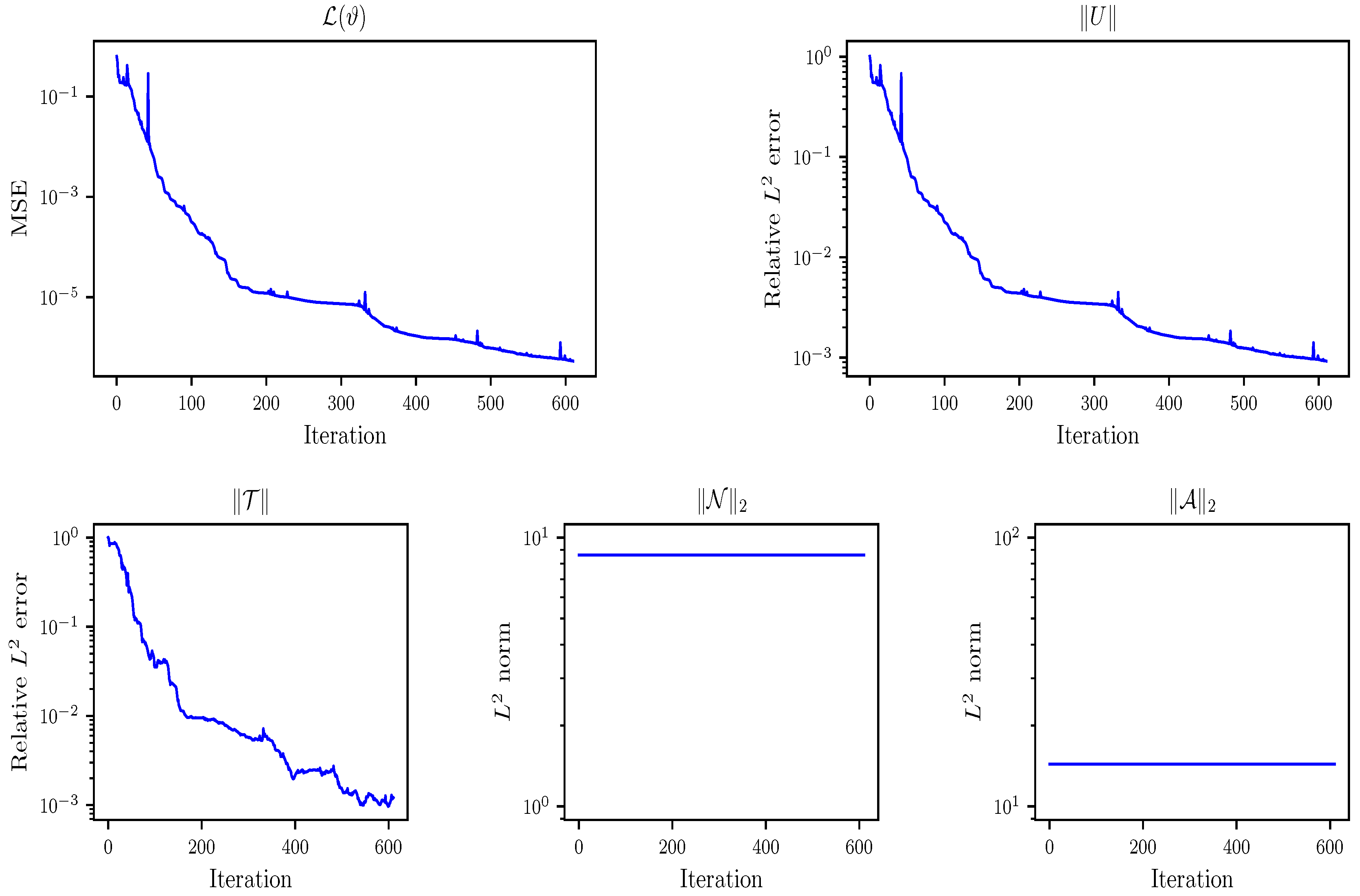
The history of the loss function L ( ϑ ) and the relative L 2 error U during the training process is presented in Figure 1. From the decreasing trend of the loss function and the error, the proposed method of decomposing the kernel function into three basis functions is validated as feasible. It also illustrates the stability of the method during the training process. Moreover, we also display the dynamic change in the relative error of the basis function T ( x ) and the L 2 norm of the basis functions N ( y ) and A ( z ) during the training process in Figure 1. It can be observed from the figure that the network T ( x ; ϑ ) provides an ideal level of prediction accuracy. Since the basis functions N ( y ) and A ( z ) are only related to y and z, respectively, their norms remain fixed during the training process. Based on the above analysis, it can be demonstrated that our proposed neural network-based variable separation method for the kernel function is reasonable.

3.2. 2D Problem

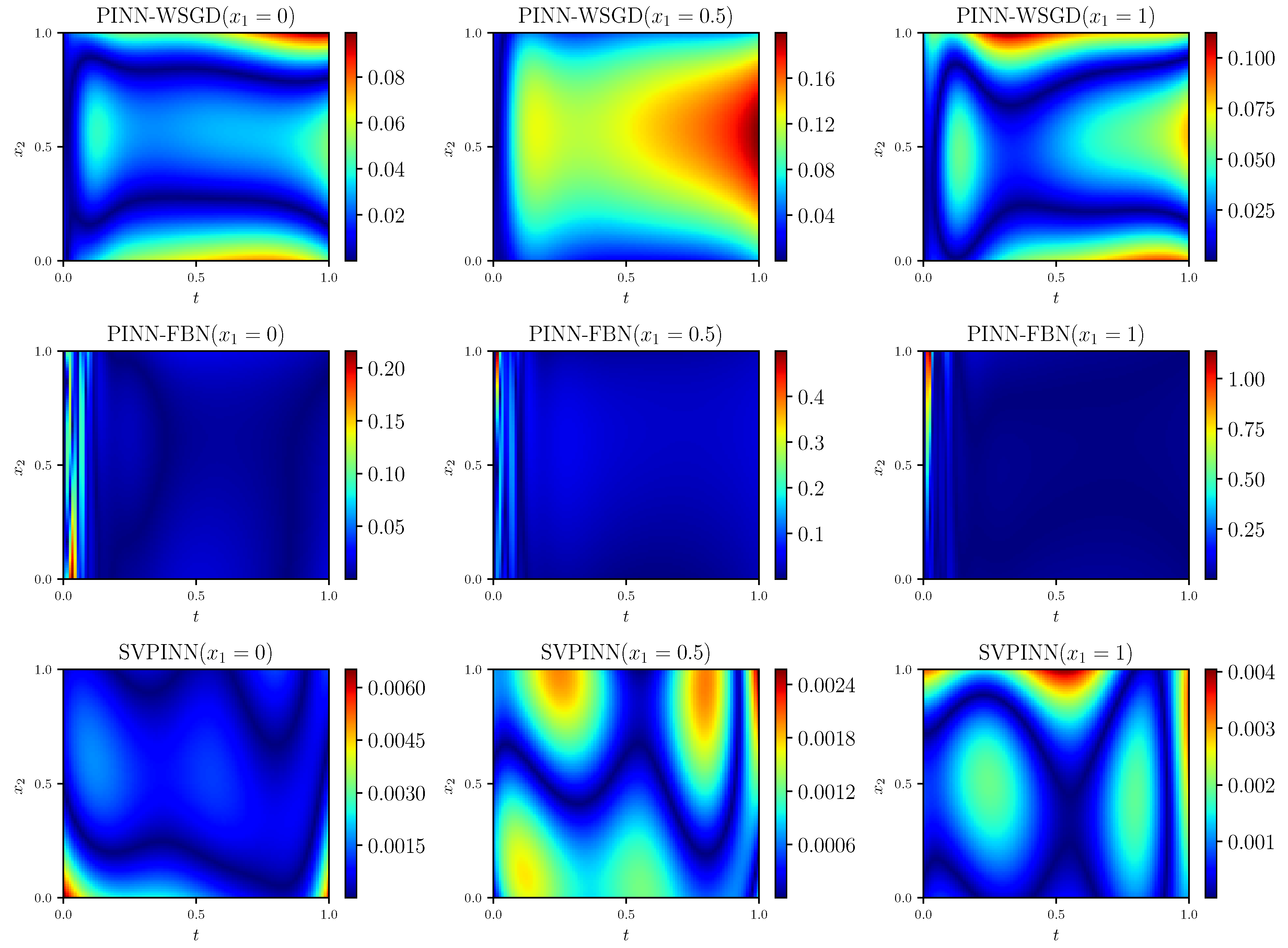
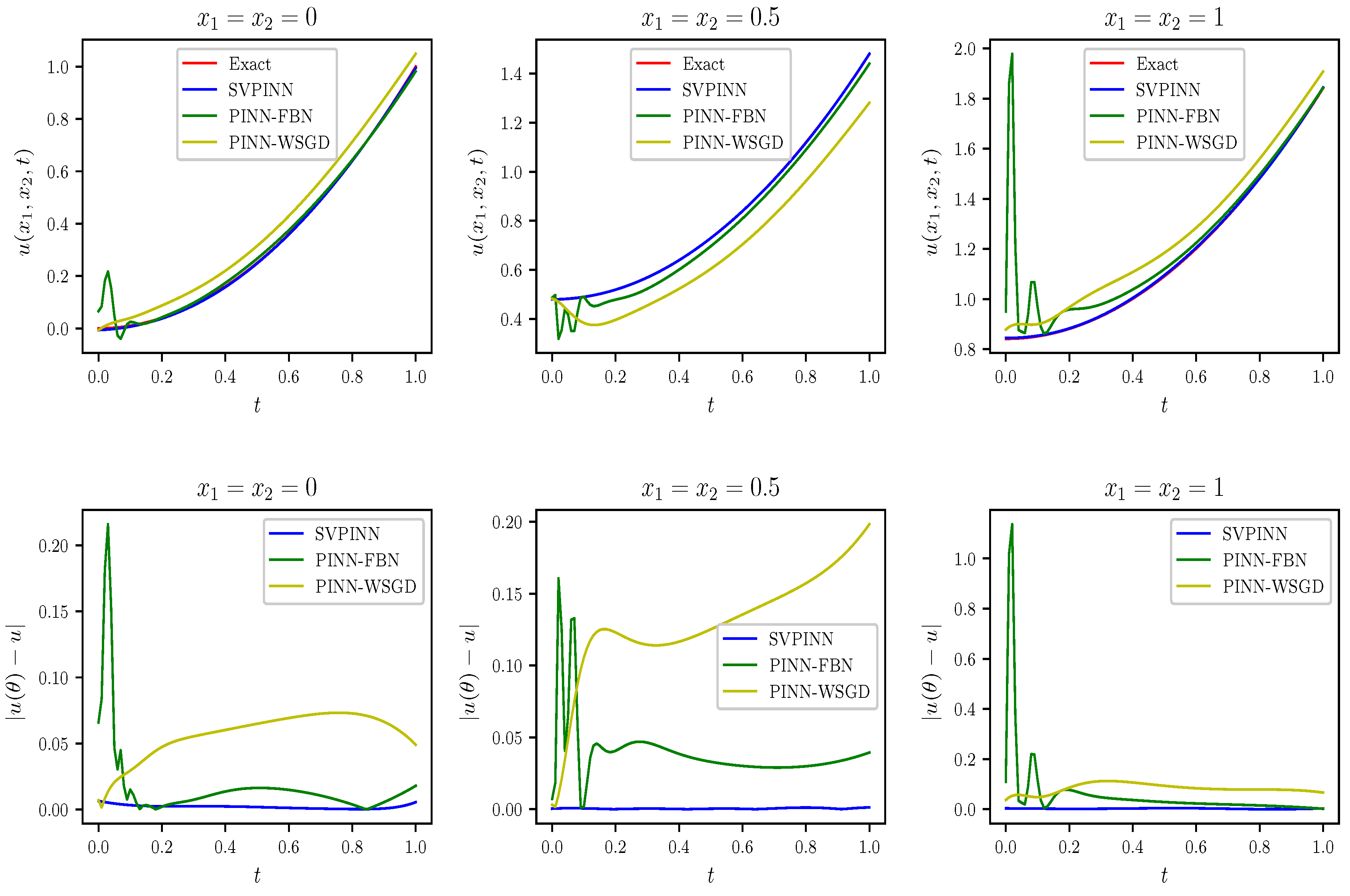
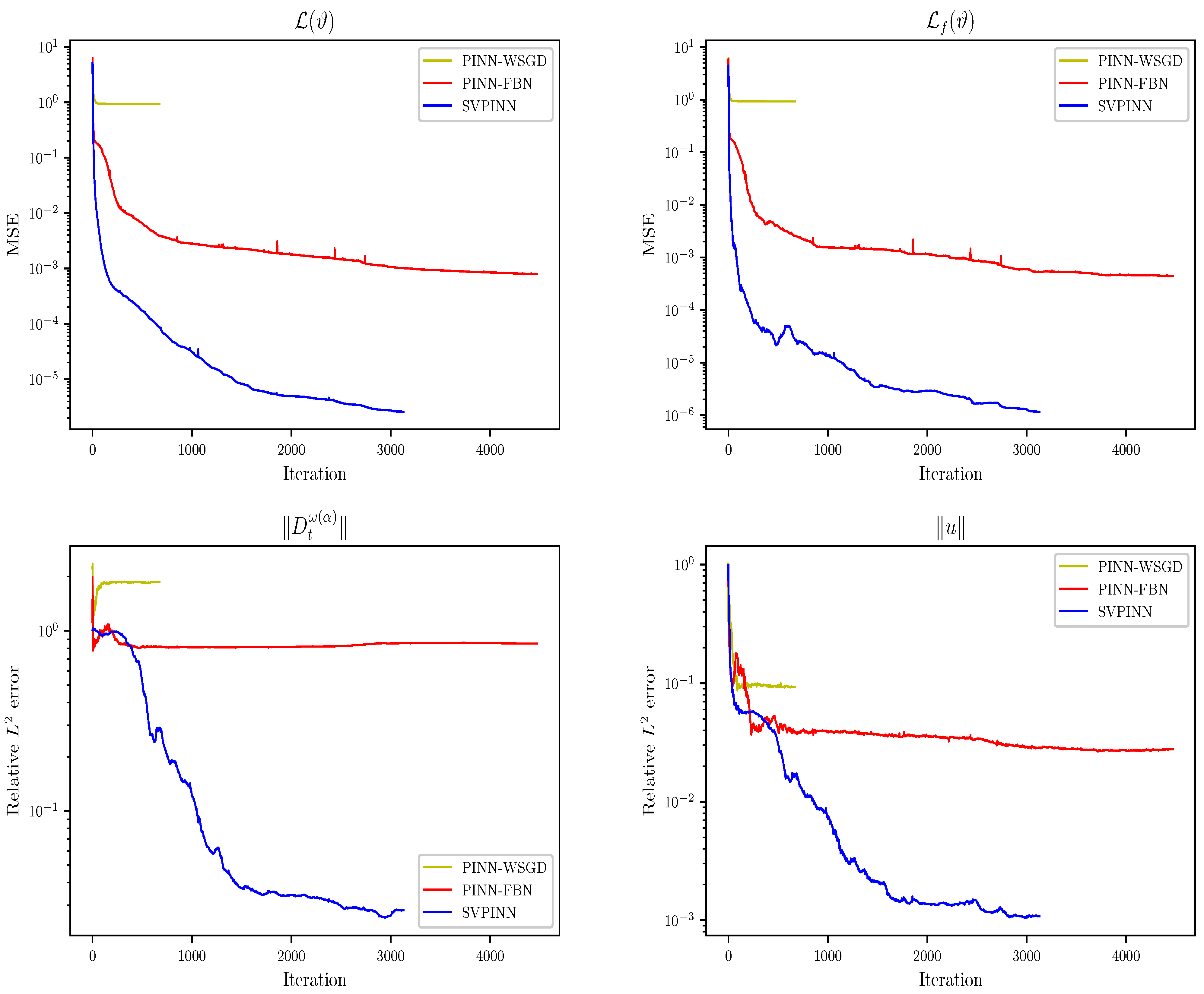
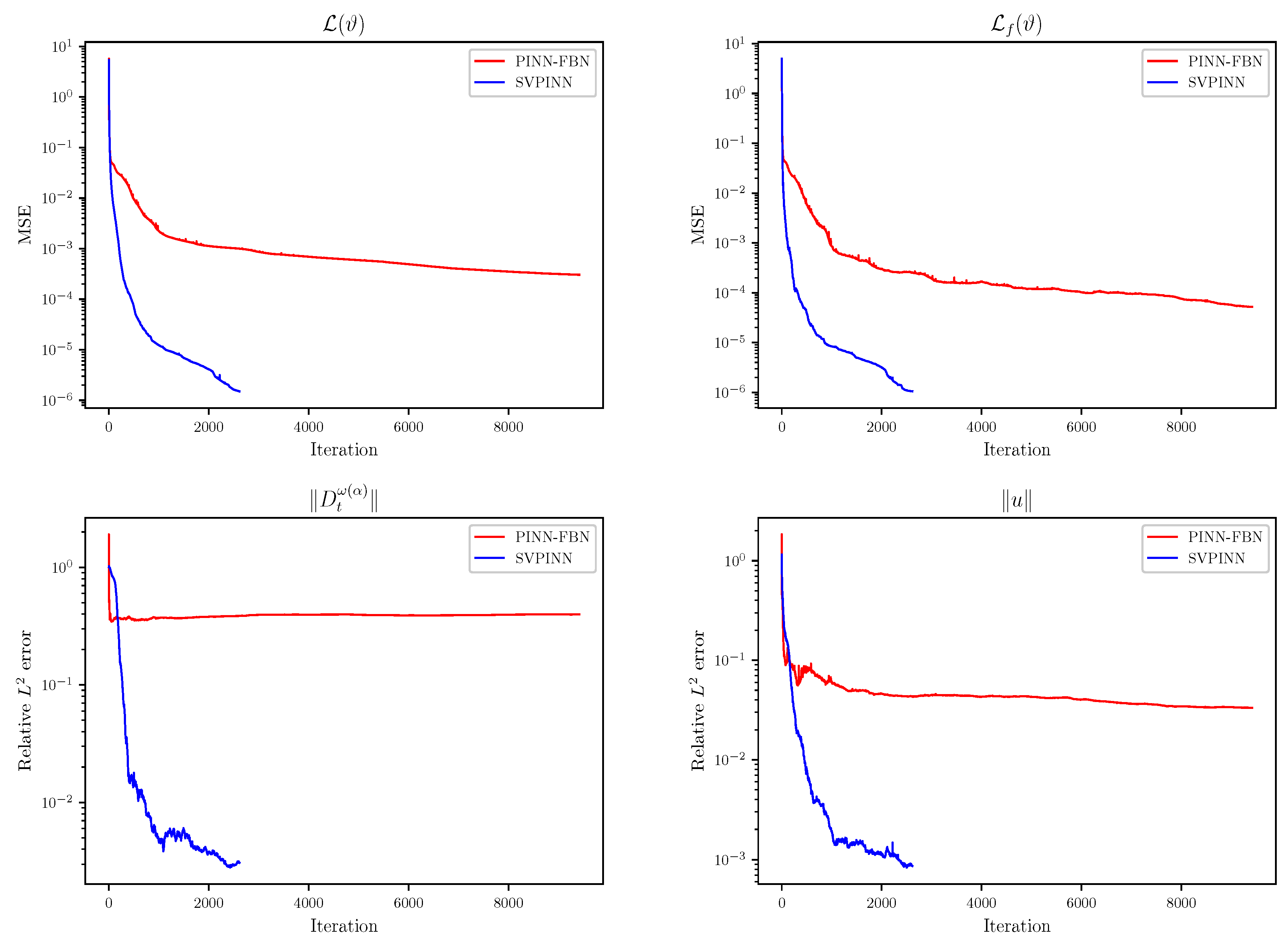
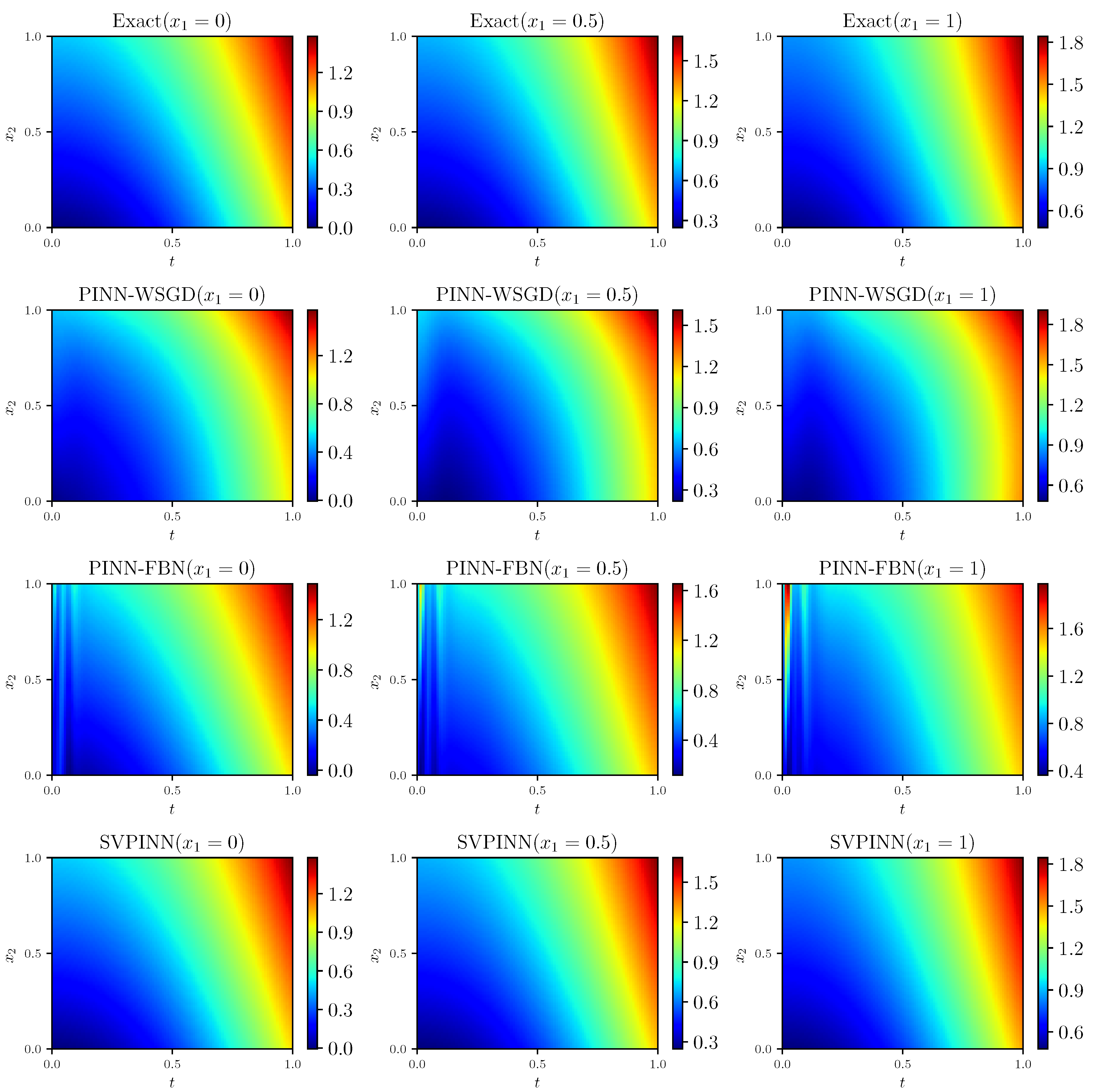
For this example, we set Ω = ( 0 , 1 ) 2 and τ = ( 0 , 1 ] . Figure 2 displays the solutions predicted by the SVPINN, PINN-FBN, and PINN-WSGD methods. Moreover, the corresponding absolute error between the predicted and exact solutions is depicted in Figure 3. It reveals that the proposed method can obtain better prediction accuracy. Figure 4 provides a more explicit comparison between the SVPINN, PINN-FBN, and PINN-WSGD, illustrating that the proposed SVPINN is closer to the exact solution. Figure 5 presents a comparative analysis of the SVPINN, PINN-WSGD, and PINN-FBN methods, which depicts the dynamic changes in the total function L ( ϑ ) , loss term L f ( ϑ ) , and relative errors. This figure demonstrates that the PINN-WSGD has poor convergence performance in solving FPDE (1), making it difficult to effectively reduce errors and achieve efficient and accurate prediction. Although the PINN-FBN can solve the problem (1), its convergence speed is relatively slow during the training process, and more iterations are required to reach the same level of accuracy. Compared to the PINN-FBN, the SVPINN exhibits better performance and faster convergence speed. It can achieve a lower mean square error with fewer iterations and achieve a more ideal prediction result.
In Table 1 and Table 2, we present our ablation study on the key components of the three PINN methods, such as the network structure and number of training points, and quantitatively analyze their impact on the accuracy, convergence speed, and generalization ability of the model by adjusting parameters. The training time represents the CPU time. From Table 1, it can be found that our proposed method significantly outperforms the PINN-FBN and PINN-WSGD methods in prediction accuracy, while maintaining comparable memory usage. In terms of convergence speed, the SVPINN has the potential to accelerate convergence under appropriate network structures. The PINN-WSGD has a short computation time but fails to achieve effective convergence, while the PINN-FBN generally takes a long time to converge.

3.3. Irregular Domain

To systematically evaluate the adaptability and solving capability of the SVPINN in complex geometric scenes
Ω = { ( x , y ) R d : x = r cos ( θ ) , y = r sin ( θ ) , θ [ 0 , 2 π ] , x 2 + y 2 r 2 } ,
we select five irregular domains as the research object. The parametric equations of these domains are as follows
r 1 = 0.6 0.2 cos ( 7 θ ) , r 2 = 1 + tanh ( cos ( 2.5 θ ) ) sin ( 5.5 θ ) , r 3 = 0.5 sin ( 5 θ ) + 1.1 sin 3 ( 5 θ ) , r 4 = 1.5 sin ( 6 θ ) + 1.1 sin 3 ( 6 θ ) , r 5 = 2 sin ( 8 θ ) + 1.1 sin 3 ( 8 θ ) .
The time interval is the same as that in Section 3.2.
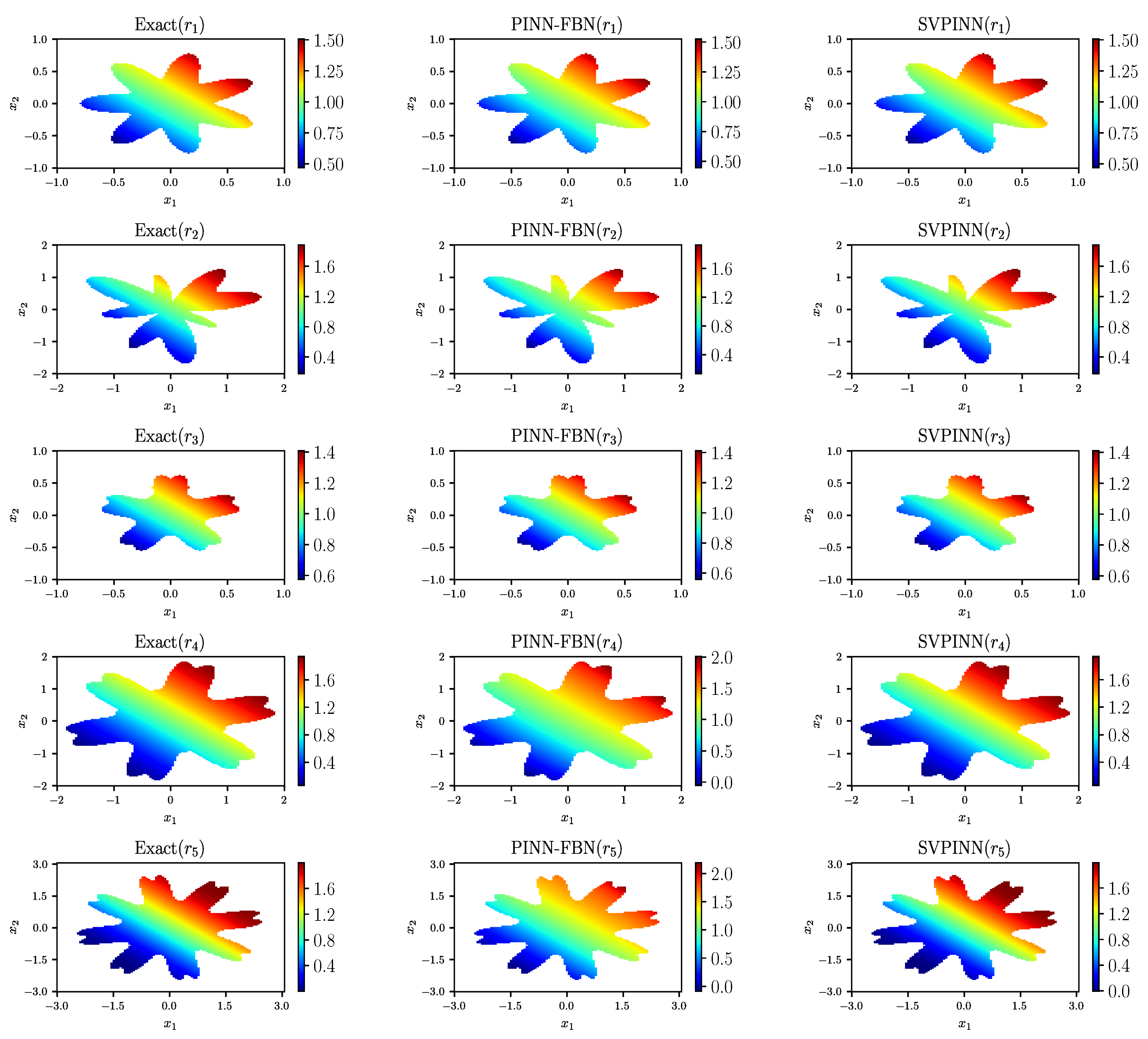
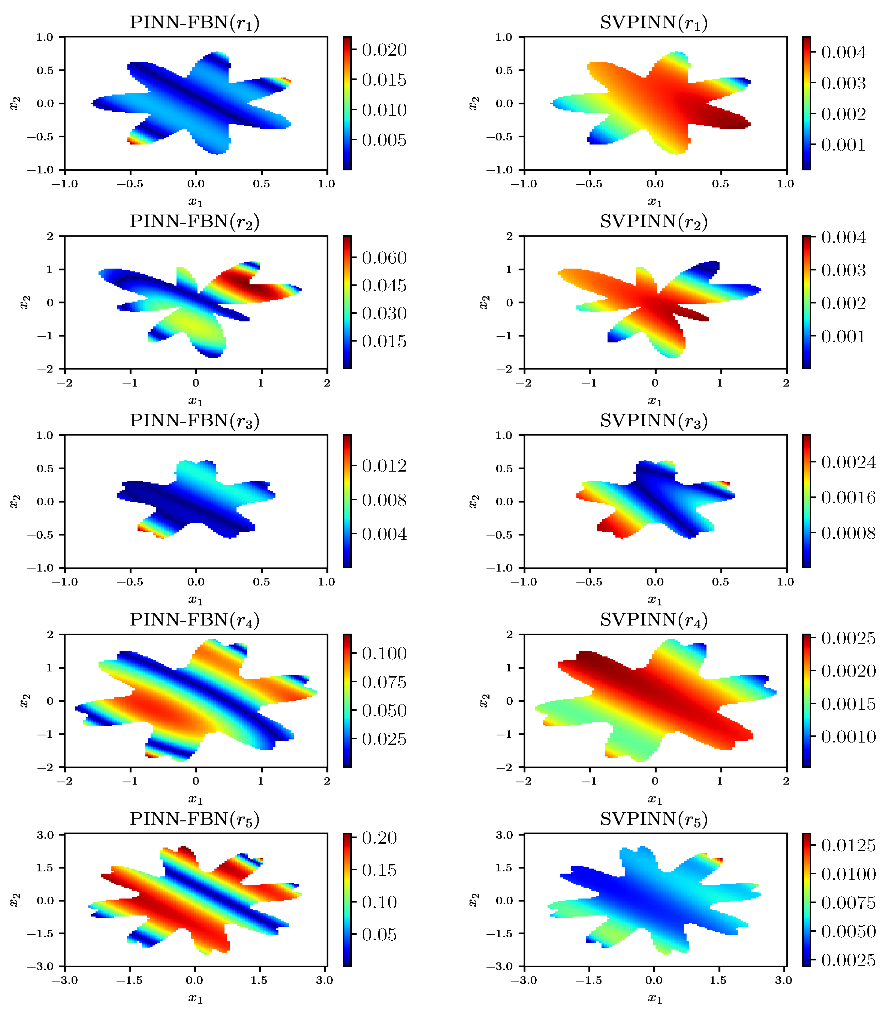
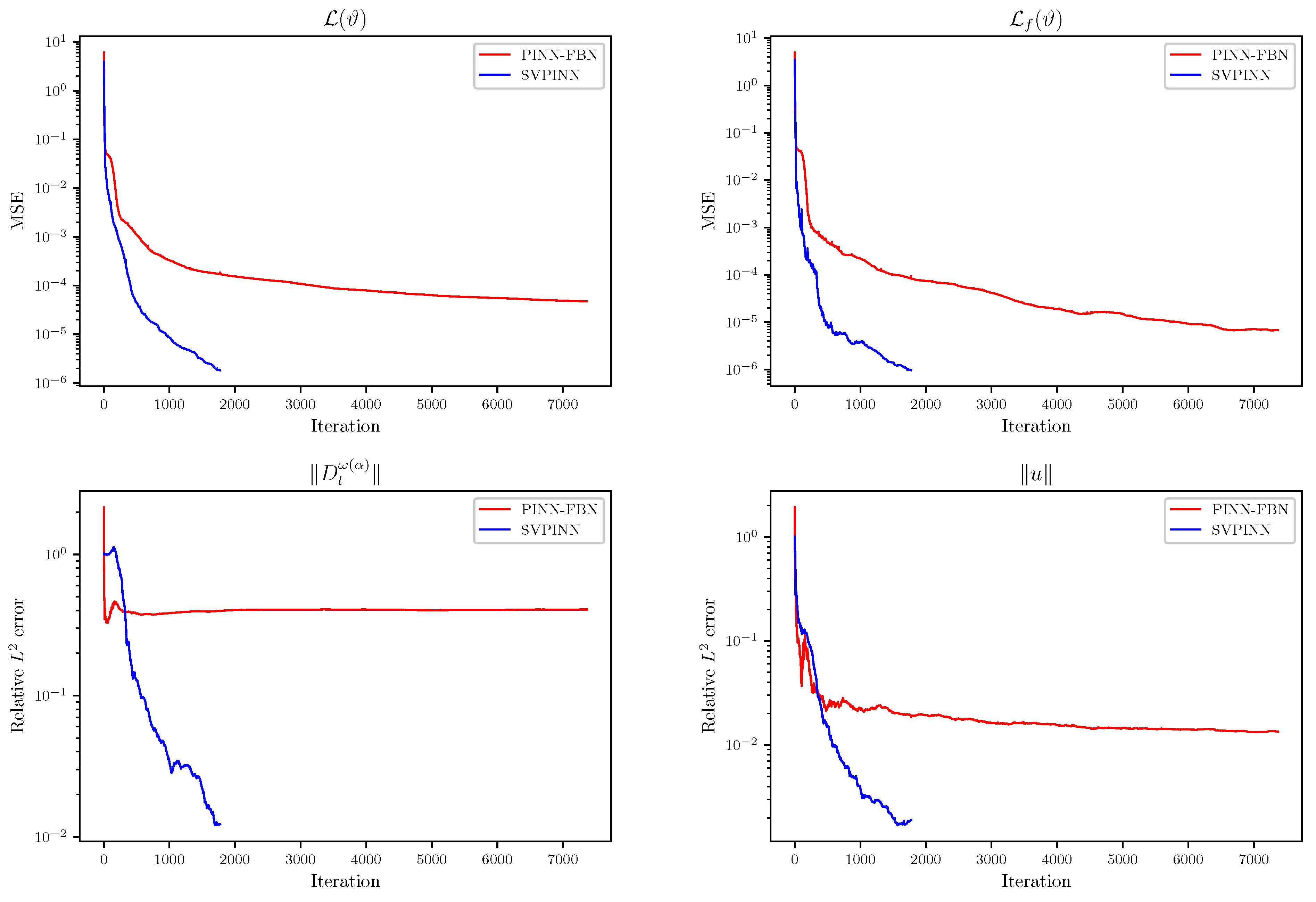
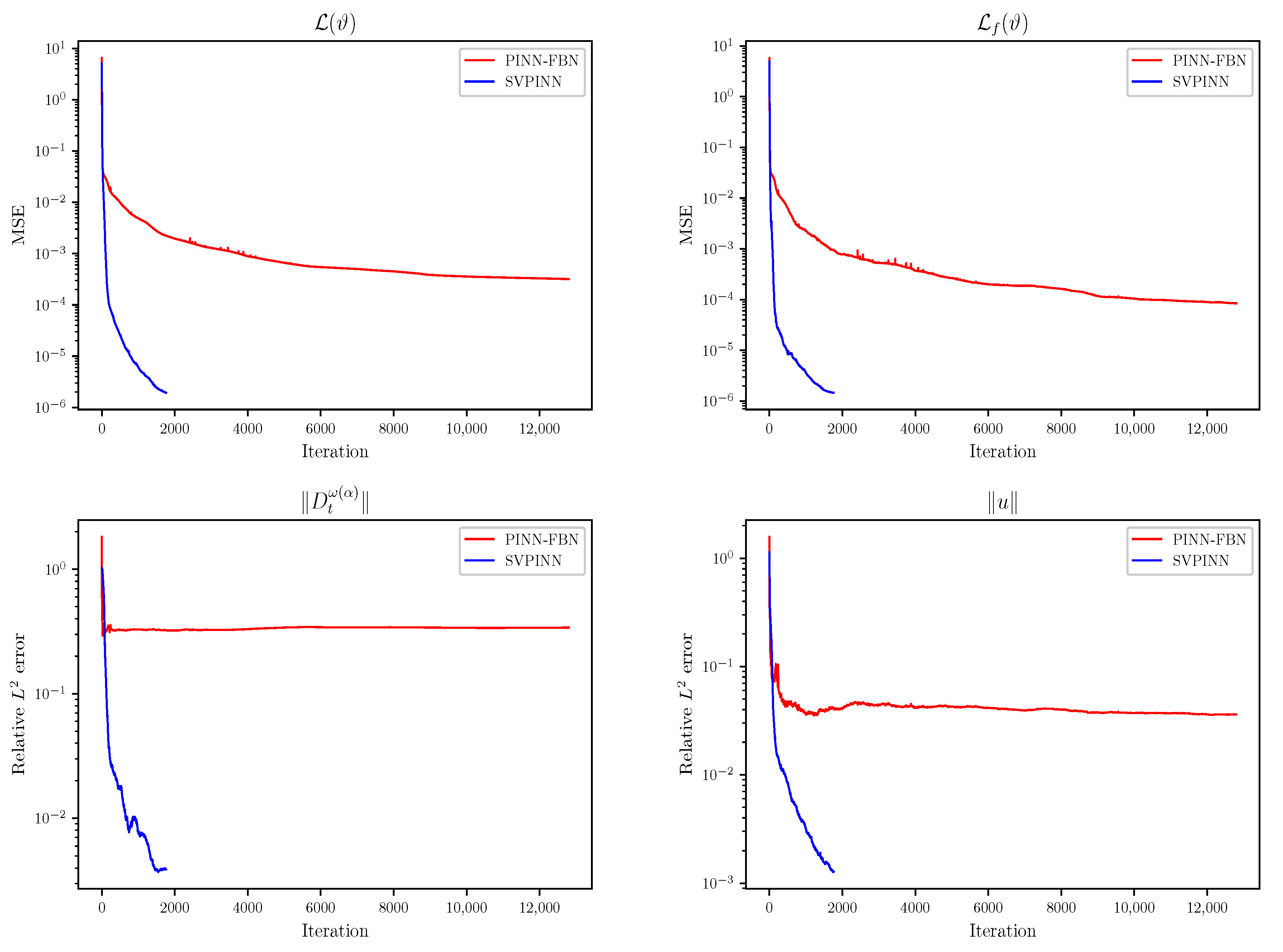
Table 3 reports the relative L 2 error and calculation cost provided by the SVPINN, the MoPINN [43], and the PINN-FBN. From the table, it can be seen that the relative error of our proposed method always remains between the levels of 10 4 and 10 3 , which are one and two orders of magnitude higher than the prediction accuracy of the other two methods. The results demonstrate that our proposed method can better predict the exact solution. Figure 6 presents the predictions given by the proposed SVPINN and the PINN-FBN, and Figure 7 displays the distribution of the absolute error between the exact solution and the prediction. From the figure, it can be observed that the prediction results of our proposed method have higher consistency with the exact solution, which intuitively verifies the effectiveness of the proposed SVPINN in solving the distributed-order advection–diffusion equation with irregular domains. To evaluate the feasibility of the SVPINN by monitoring the changes in the loss function during the training process and demonstrate physical consistency via a quantitative analysis of the residual equation and the errors, Figure 8, Figure 9, Figure 10, Figure 11 and Figure 12 display the decreasing trend of the loss function L ( ϑ ) , the loss term L f ( ϑ ) , and the relative errors of the distributed-order derivative D t ω ( α ) and the exact solution u ( x , t ) in the process of optimizing the network. In general, the SVPINN has more advantages in the optimization effect. It not only performs better than the PINN-FBN in reducing the loss, but also converges faster and can reach a lower error level. Moreover, we also test the impact of network parameters, the number of collocation points, and the number of the initial and boundary points on the performance of the SVPINN in Table 4, Table 5, Table 6 and Table 7. From the table, it can be seen that the relative error of the SVPINN is generally maintained at the level of 10 3 to 10 4 , which are one and two orders of magnitude lower than the other two methods. The SVPINN has excellent advantages in computational efficiency. The data in the table clearly indicates that the training time required by the SVPINN is significantly shorter than that of the PINN-FBN, often as little as 10 % or even less. Furthermore, the SVPINN achieves higher accuracy without incurring additional memory consumption, maintaining essentially the same memory usage as the PINN-FBN. When the hyperparameters change, the error of the SVPINN consistently stays at the order of 10 3 , indicating its strong stability.

3.4. High-Dimensional Problems

In this example, we investigate the effectiveness of the SVPINN for high-dimensional distributed-order advection–diffusion equation. The spatial domain and time interval are set to Ω = ( 1 , 1 ) d and τ = ( 0 , 1 ] , respectively.
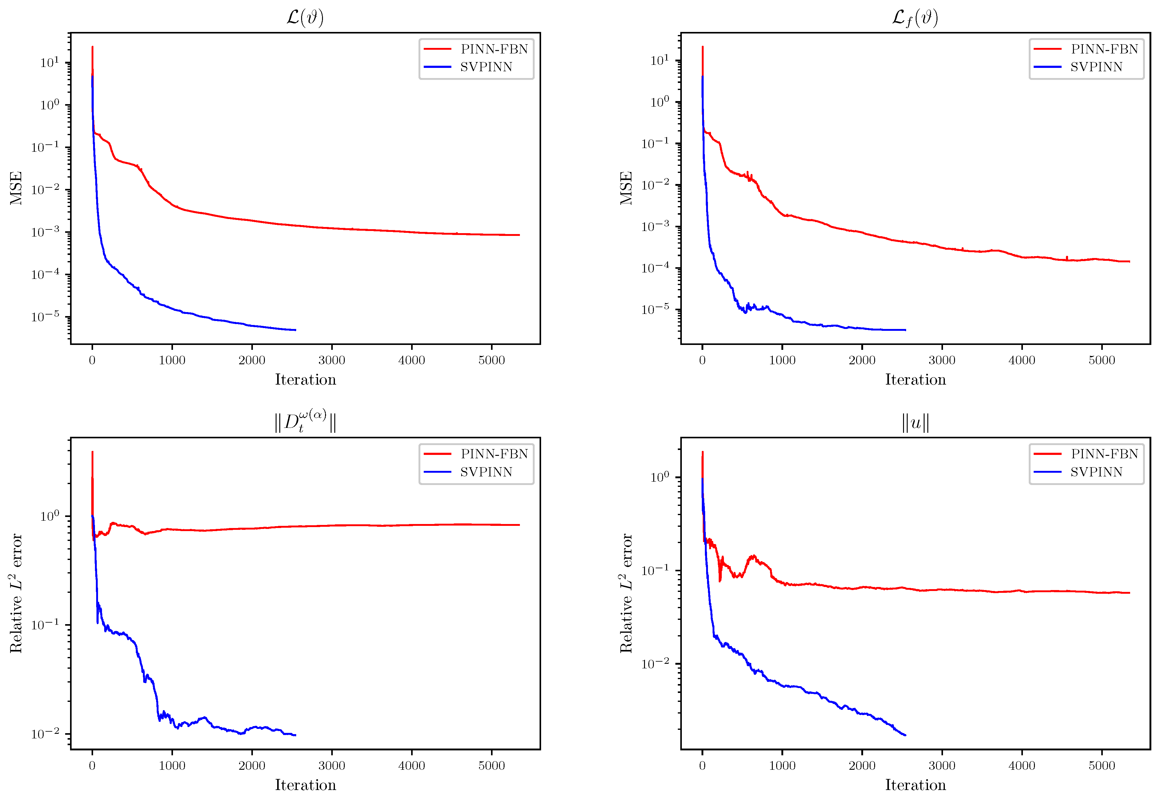
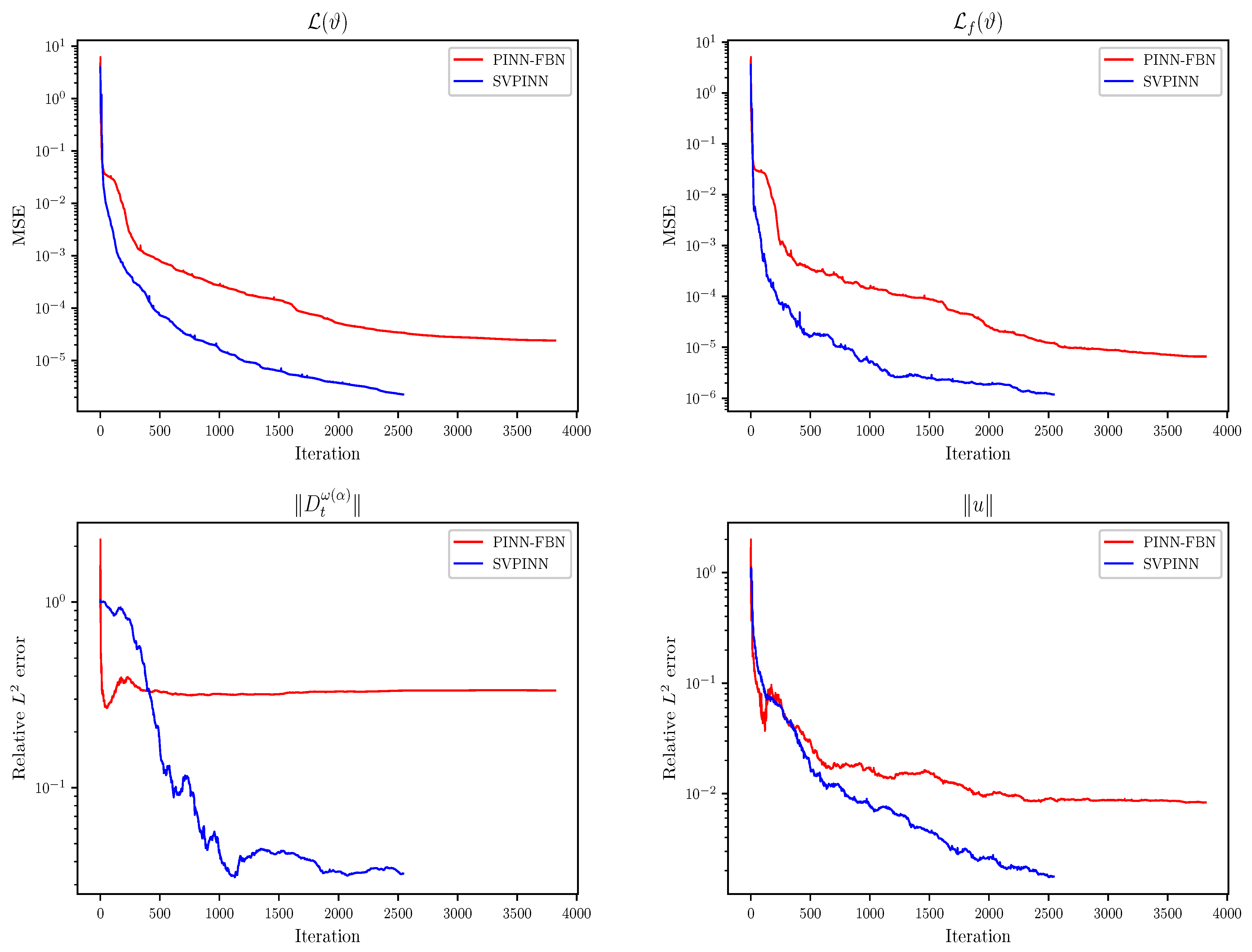
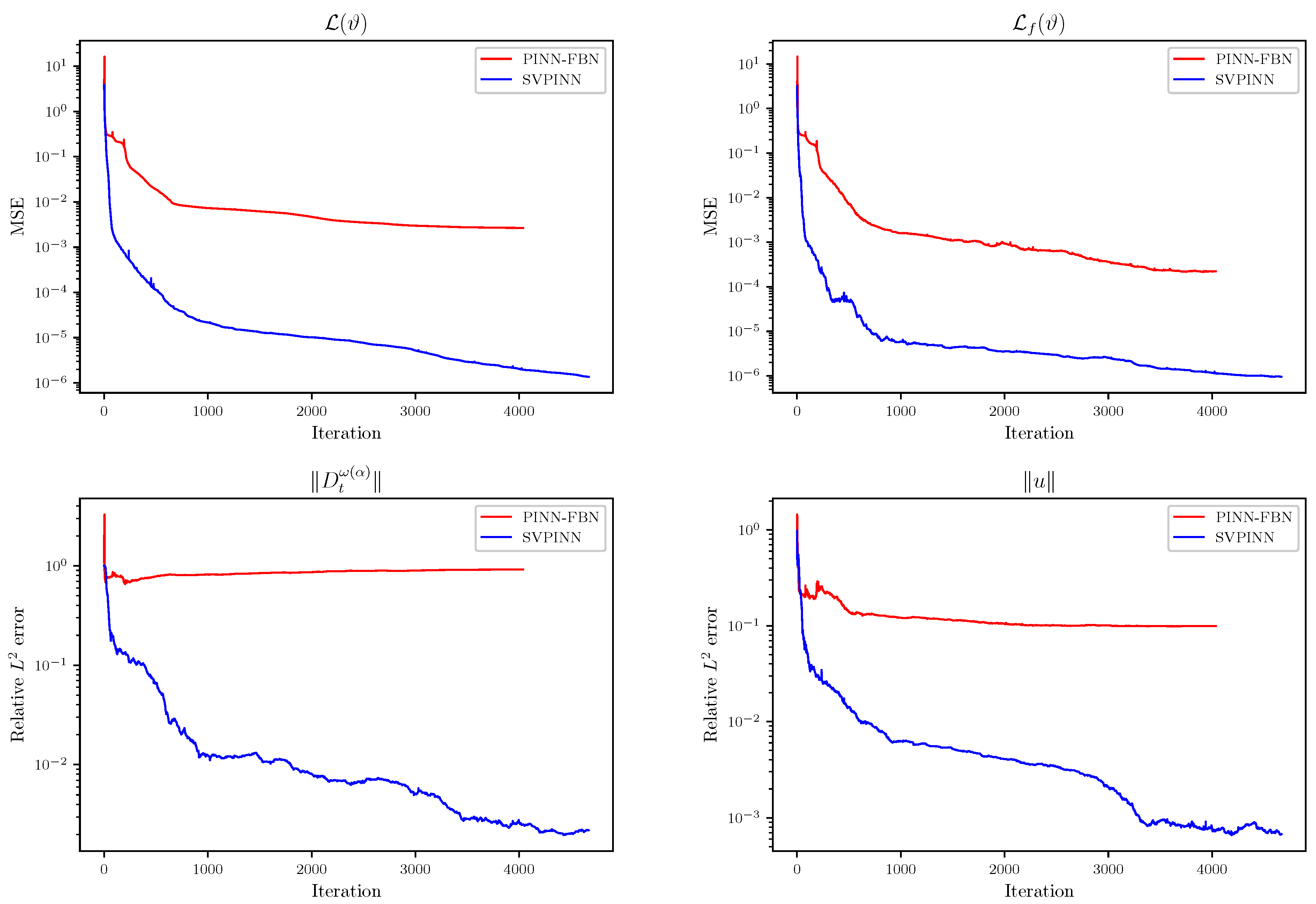
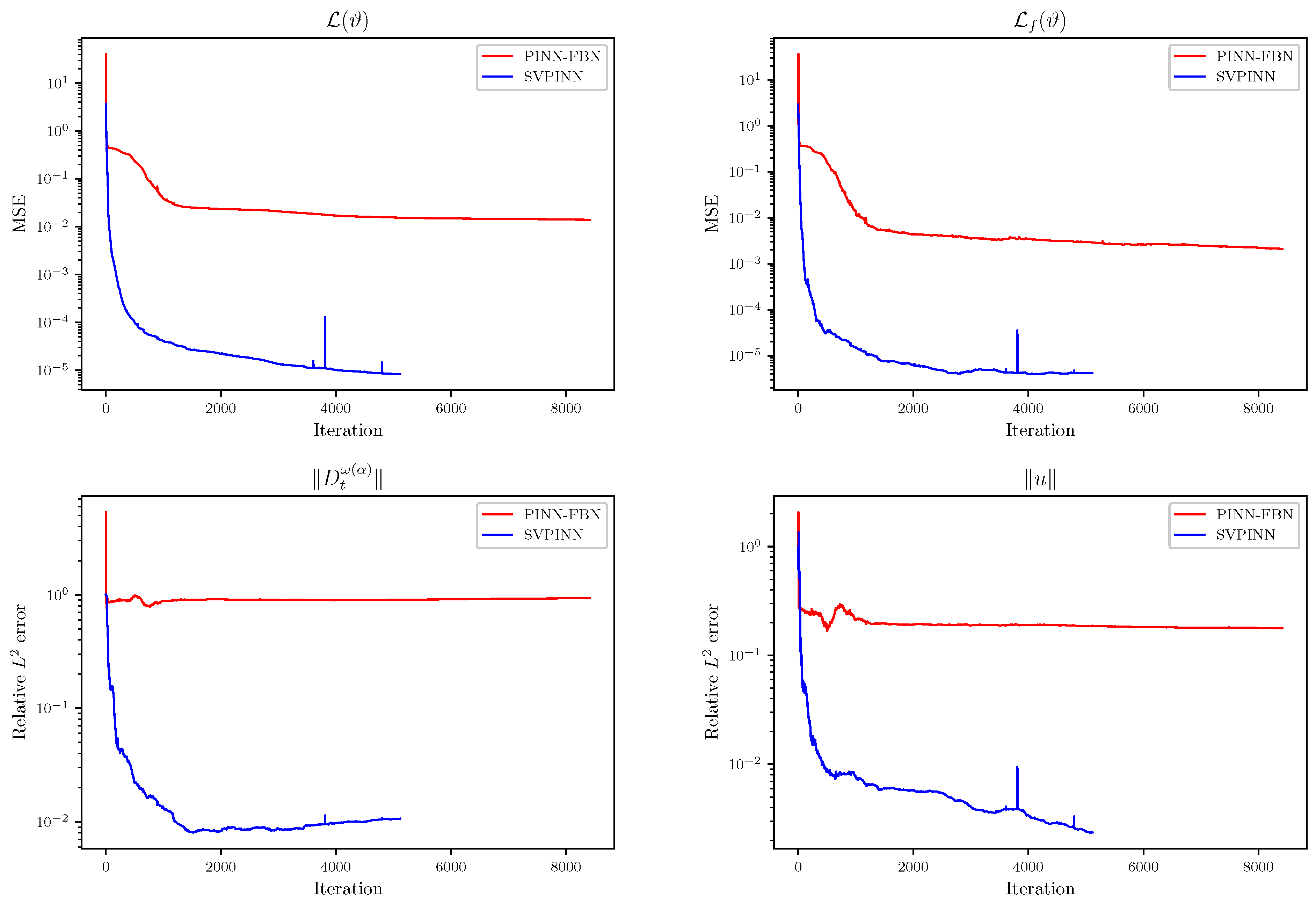
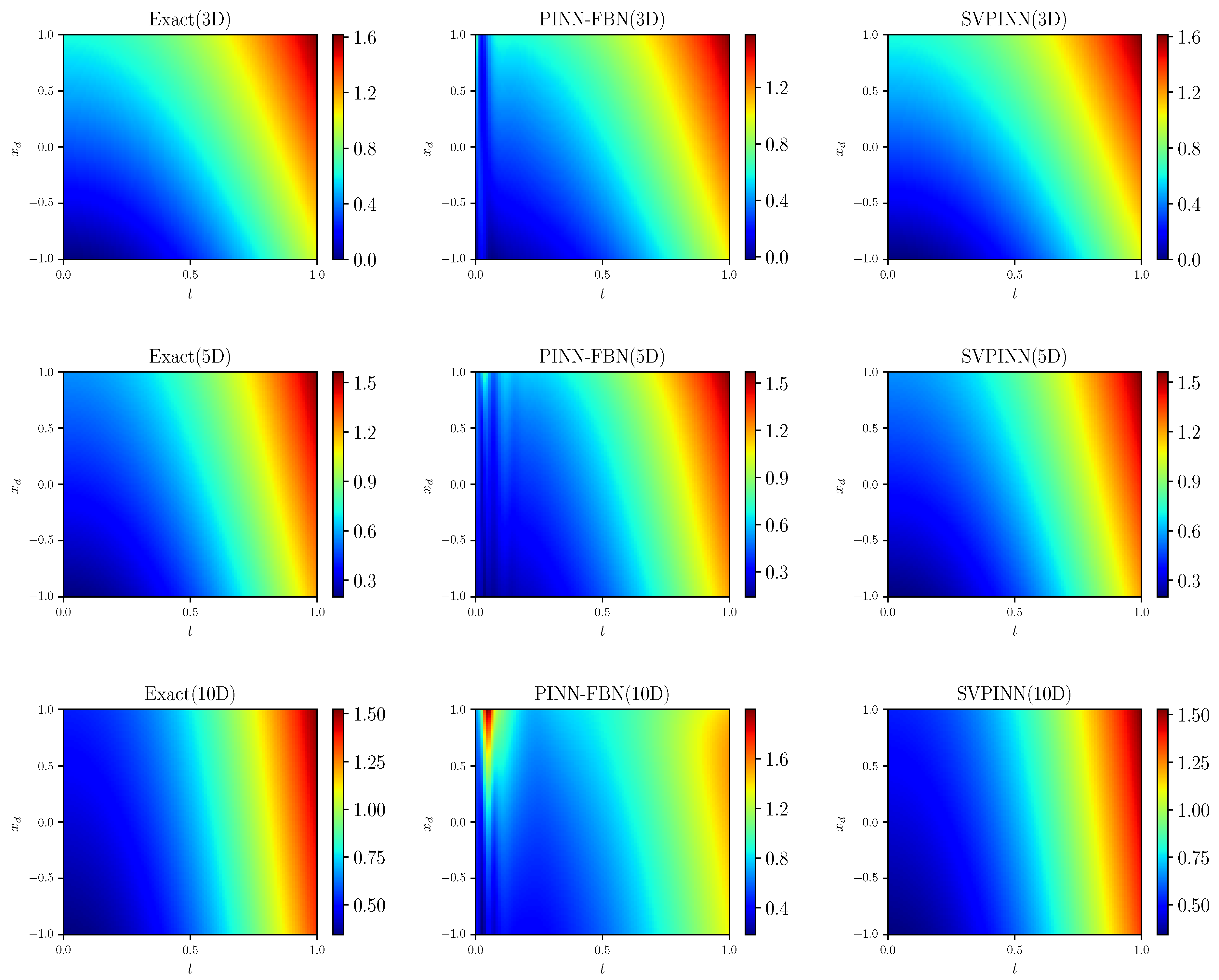
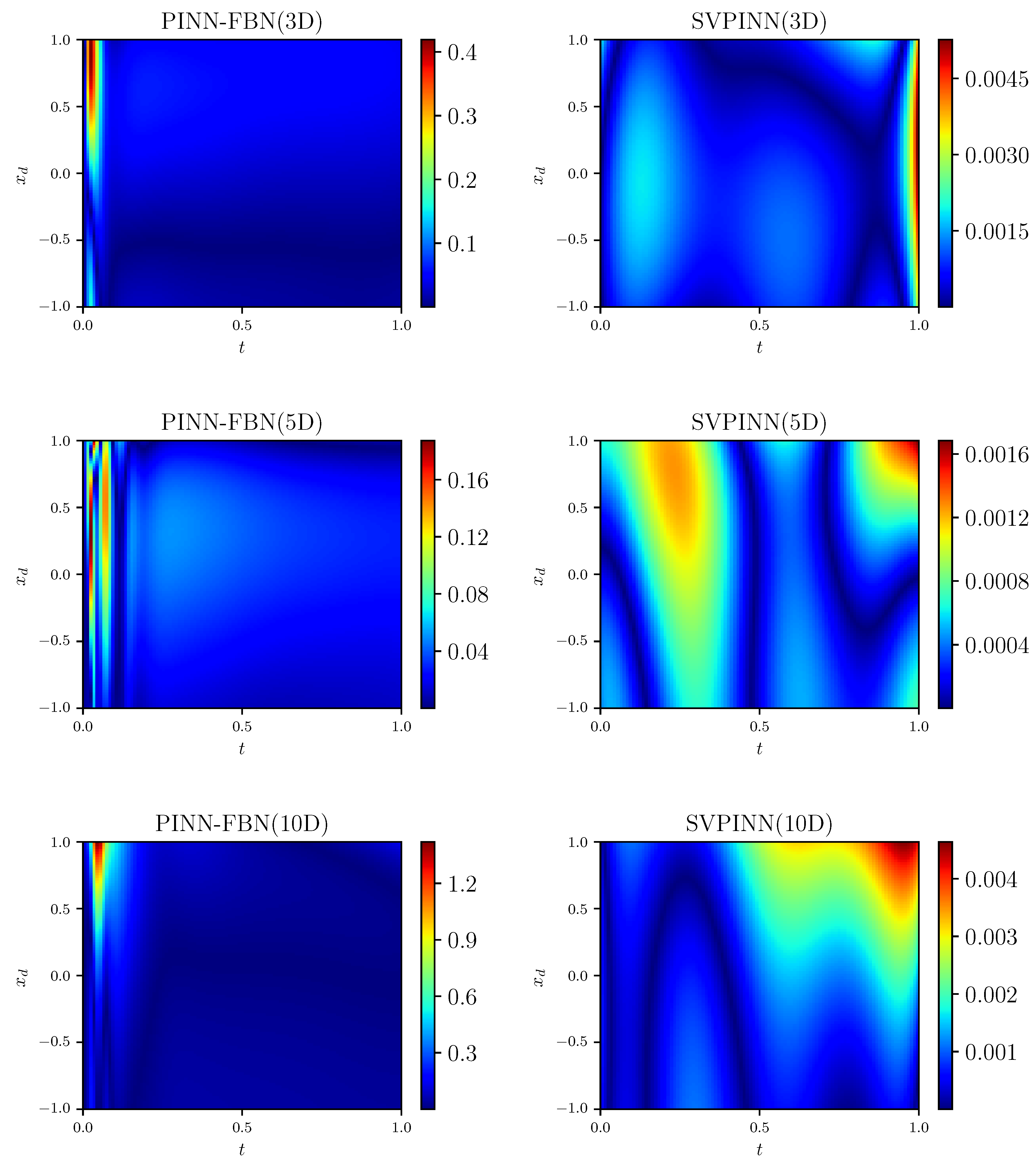
In Table 8, we present the relative L 2 error, training time, and memory usage obtained by the SVPINN and PINN-FBN methods at d = 3 , 5 , 10 . The error between the exact solution and the prediction given by the SVPINN is 1.351 × 10 3 , when d = 10 . The results demonstrate that for high-dimensional cases, our proposed method also has good prediction accuracy. In Figure 13 and Figure 14, we plot the distributions of the analytical solution, the prediction, and the absolute error. In addition, we provide a comparison of the loss and relative error between the SVPINN and PINN-FBN methods in Figure 15, Figure 16 and Figure 17, which shows that the SVPINN has higher accuracy in approximating the distributed-order derivative and can better optimize the network parameters. During the training process, we can observe a stable decrease and rapid convergence of the total loss function, demonstrating the feasibility of the proposed SVPINN. Quantitative analysis of the loss of the residual equation and the relative error, as shown in the figures, verifies that the neural network adheres to the physical laws described by the governing equation during the training process. Table 9, Table 10, Table 11 and Table 12 report the performance of the SVPINN and PINN-FBN methods with respect to the network structure, the number of collocation points, and the number of initial and boundary data. From the table, it can be seen that the prediction accuracy of the PINN-FBN is maintained at the level of 10 2 , while that of the SVPINN is maintained at the level of 10 3 . The training time for the SVPINN is generally maintained between 20 s and 100 s, while the PINN-FBN requires approximately 60 s to 800 s, which is 3 to 8 times longer than the SVPINN. When the network structure and the number of training points change, the prediction accuracy of the SVPINN remains almost stable at the level of 10 3 , demonstrating strong robustness.

3.5. Comprehensive Analysis

In this section, to further comprehensively evaluate the performance and the computational complexity of the proposed method, we summarized, in Table 13, the key indicators such as prediction accuracy, computation time, and memory, which reflect the overall performance of SVPINN in Section 3.2, Section 3.3 and Section 3.4. As shown in the table, in Section 3.2, Section 3.3 and Section 3.4, our proposed method not only achieves better prediction accuracy, but also has lower memory consumption than the PINN-FBN. Moreover, the SVPINN significantly improves computational efficiency with similar computational costs, reducing training time to 16 % to 50 % of that required by the PINN-FBN. Although the PINN-WSGD has less training time than the SVPINN, it fails to accurately predict the exact solution. Overall, our proposed method shows better performance in both prediction accuracy and computational cost, while also exhibiting lower computational complexity and excellent scalability.
4. Conclusions

In this work, we proposed a novel PINN framework and applied it to solve the distributed-order advection–diffusion equation. In the SVPINN framework, we separate the time variable and the other two integration variables in the kernel function of the Caputo integral into three independent functions, transforming the kernel function into the product of these functions. Further, we change the integral form by defining two functions determined by the integral variables α and η and use the network to approximate the function related only to the time variable. In the proposed PINN method, the solution process of the distributed-order derivative is embedded into the network training framework, and an adaptive learning mode based on neural network parameter training is adopted to approximate the distributed-order derivative term. Several numerical experiments are carried out to verify the effectiveness of the SVPINN method. The results demonstrate that the integral scheme we constructed can effectively approximate the distributed-order derivative, and it makes the proposed SVPINN model achieve higher accuracy than the PINN models that use the numerical schemes, such as the FBN- θ scheme or the WSGD scheme, to discretize the fractional derivative. The focus of future research is to enhance the ability of the SVPINN model to deal with more complex physical systems, such as fractional underground seepage problems with complex mixed boundary conditions.

Author Contributions

Methodology, W.L. and Y.L.; software, W.L.; validation, W.L. and Y.L.; writing—original draft preparation, W.L.; writing—review and editing, Y.L. All authors have read and agreed to the published version of the manuscript.

Funding

This work was supported by the National Natural Science Foundation of China (12061053), the Young Innovative Talents Project of Grassland Talents Project, and the Program for Innovative Research Team in Universities of Inner Mongolia Autonomous Region (NMGIRT2413).

Data Availability Statement

The data that support the findings of this study are yielded by using our method.

Conflicts of Interest

The authors declare no conflicts of interest.

Appendix A. Two Discrete Schemes

Defining Δ α = 1 H and Δ t = T N t , we set α i = i Δ α for i = 0 , 1 , 2 , , H , and t n = n Δ t ( n = 0 , 1 , 2 , , N t ) . Without loss of generality, we fix H = 500 and N t = 20 .

Appendix A.1. FBN-θ Scheme [43,45,46,47]

The discrete scheme in the time direction of the distributed-order derivative D t ω ( α ) u ( x , t ) is as follows
D t ω ( α ) u ( x , t n + 1 2 ) = D t ω ( α ) u n + 1 + D t ω ( α ) u n 2 + O ( Δ t 2 ) = 1 2 s = 0 n + 1 β s n + 1 u s + O ( Δ t 2 + Δ α 2 ) ,
where
β s n + 1 = κ ^ n s + κ ^ n + 1 s , 0 s < n + 1 , κ ^ 0 , s = n + 1 ,
and
κ ^ n s = i = 0 2 I φ i Δ t α i κ n s ( α i ) , φ i = Δ α ω ( α i ) c i , c i = 1 2 , i = 0 , H , 1 , o t h e r w i s e .
The parameter κ i ( α ) denotes the coefficient of FBN- θ ( θ [ 1 2 , 1 ] ) , which is defined as
κ i ( α ) = 2 α ( 1 + α θ ) ( 3 2 θ ) α , i = 0 , ϕ 0 κ 0 ( α ) ψ 0 , i = 1 , 1 2 ψ 0 [ ( ϕ 0 ψ 1 ) κ 1 ( α ) + ϕ 1 κ 0 ( α ) ] , i = 2 , 1 i ψ 0 j = 1 3 [ ϕ j 1 ( i j ) ψ j ] κ i j ( α ) , i 3 ,
where
ϕ i = 2 α ( θ 1 ) ( α θ + 1 ) + α θ ( θ 3 2 ) , i = 0 , α ( 2 θ 2 3 α θ + 4 α θ 2 1 ) , i = 1 , α θ ( 1 2 θ + α 2 α θ ) , i = 2 ,
and
ψ i = 1 2 ( 3 2 θ ) ( 1 + α θ ) , i = 0 , α θ 2 ( 3 2 θ ) 2 ( 1 θ ) ( α θ + 1 ) , i = 1 , 1 2 ( 2 θ 1 ) ( α θ + 1 ) 2 α θ ( θ 1 ) , i = 2 , 1 2 α θ ( 1 2 θ ) .

Appendix A.2. WSGD Scheme [48,49]

The discrete scheme is formulated as
D t ω ( α ) u ( x , t n + 1 ) Δ α i = 0 H c i ω ( α i ) D Δ t α i u ( x , t n + 1 ) ,
where
D Δ t α i u ( x , t n + 1 ) = Δ t α j = 0 n + 1 λ j ( α ) u ( x , t n + 1 j ) , c i = 1 2 , i = 0 , H , 1 , otherwise ,
and
λ 0 ( α ) = 2 + α 2 g 0 ( α ) , λ j ( α ) = 2 + α 2 g j ( α ) α 2 g j 1 ( α ) , j 1 , g j ( α ) = ( 1 ) j α j , j 0 .

References

  1. Raissi, M.; Perdikaris, P.; Karniadakis, G.E. Physics-informed neural networks: A deep learning framework for solving forward and inverse problems involving nonlinear partial differential equations. J. Comput. Phys. 2019, 378, 686–707. [Google Scholar] [CrossRef]
  2. He, Q.; Solano, D.B.; Tartakovsky, G.; Tartakovsky, A.M. Physics-informed neural networks for multiphysics data assimilation with application to subsurface transport. Adv. Water Resour. 2020, 141, 103610. [Google Scholar] [CrossRef]
  3. Bandai, T.; Ghezzehei, T.A. Forward and inverse modeling of water flow in unsaturated soils with discontinuous hydraulic conductivities using physics-informed neural networks with domain decomposition. Hydrol. Earth Syst. Sci. 2022, 26, 4469–4495. [Google Scholar] [CrossRef]
  4. Almajid, M.M.; Abu-Al-Saud, M.O. Prediction of porous media fluid flow using physics informed neural networks. J. Pet. Sci. Eng. 2022, 208, 109205. [Google Scholar] [CrossRef]
  5. Zhu, Q.; Liu, Z.; Yan, J. Machine learning for metal additive manufacturing: Predicting temperature and melt pool fluid dynamics using physics-informed neural networks. Comput. Mech. 2021, 67, 619–635. [Google Scholar] [CrossRef]
  6. Zhang, R.; Liu, Y.; Sun, H. Physics-informed multi-LSTM networks for metamodeling of nonlinear structures. Comput. Meth. Appl. Mech. Eng. 2020, 369, 113226. [Google Scholar] [CrossRef]
  7. Singh, V.; Harursampath, D.; Dhawan, S.; Sahni, M.; Saxena, S.; Mallick, R. Physics-informed neural network for solving a one-dimensional solid mechanics problem. Modelling 2024, 5, 1532–1549. [Google Scholar] [CrossRef]
  8. Pratap, V.; Kumar, P.; Rao, C.; Gilchrist, M.D.; Tripathi, B.B. Modelling fourth-order hyperelasticity in soft solids using physics informed neural networks without labelled data. Brain Res. Bull. 2025, 224, 111318. [CrossRef]
  9. Jalili, D.; Jang, S.; Jadidi, M.; Giustini, G.; Keshmiri, A.; Mahmoudi, Y. Physics-informed neural networks for heat transfer prediction in two-phase flows. Int. J. Heat Mass Transf. 2024, 221, 125089. [Google Scholar] [CrossRef]
  10. Laubscher, R. Simulation of multi-species flow and heat transfer using physics-informed neural networks. Phys. Fluids 2021, 33, 087101. [Google Scholar] [CrossRef]
  11. Goswami, S.; Anitescu, C.; Chakraborty, S.; Rabczuk, T. Transfer learning enhanced physics informed neural network for phase-field modeling of fracture. Theor. Appl. Fract. Mech. 2020, 106, 102447. [Google Scholar] [CrossRef]
  12. Sitzmann, V.; Martel, J.; Bergman, A.; Lindell, D.; Wetzstein, G. Implicit neural representations with periodic activation functions. Adv. Neural Inf. Process. Syst. 2020, 33, 7462–7473. [Google Scholar]
  13. Saragadam, V.; LeJeune, D.; Tan, J.; Balakrishnan, G.; Veeraraghavan, A.; Baraniuk, R.G. Wire: Wavelet implicit neural representations. arXiv 2023, arXiv:2301.05187. [Google Scholar]
  14. Moseley, B.; Markham, A.; Nissen-Meyer, T. Finite basis physics-informed neural networks (FBPINNs): A scalable domain decomposition approach for solving differential equations. arXiv 2021, arXiv:2107.07871. [Google Scholar] [CrossRef]
  15. Ainsworth, M.; Dong, J. Galerkin neural network approximation of singularly-perturbed elliptic systems. Comput. Meth. Appl. Mech. Eng. 2022, 402, 115169. [Google Scholar] [CrossRef]
  16. Gao, H.; Sun, L.; Wang, J.X. PhyGeoNet: Physics-informed geometry-adaptive convolutional neural networks for solving parameterized steady-state PDEs on irregular domain. J. Comput. Phys. 2021, 428, 110079. [Google Scholar] [CrossRef]
  17. Rodriguez-Torrado, R.; Ruiz, P.; Cueto-Felgueroso, L.; Green, M.C.; Friesen, T.; Matringe, S.; Togelius, J. Physics-informed attention-based neural network for solving non-linear partial differential equations. arXiv 2021, arXiv:2105.07898. [Google Scholar]
  18. Wight, C.L.; Zhao, J. Solving Allen-Cahn and Cahn-Hilliard equations using the adaptive physics informed neural networks. Commun. Comput. Phys. 2021, 29, 930–954. [Google Scholar] [CrossRef]
  19. Wang, S.; Teng, Y.; Perdikaris, P. Understanding and mitigating gradient flow pathologies in physics-informed neural networks. SIAM J. Sci. Comput. 2021, 43, A3055–A3081. [Google Scholar] [CrossRef]
  20. Wang, S.; Yu, X.; Perdikaris, P. When and why PINNs fail to train: A neural tangent kernel perspective. J. Comput. Phys. 2022, 449, 110768. [Google Scholar] [CrossRef]
  21. Meer, R.V.D.; Oosterlee, C.W.; Borovykh, A. Optimally weighted loss functions for solving PDEs with neural networks. J. Comput. Appl. Math. 2022, 405, 113887. [Google Scholar] [CrossRef]
  22. Xiang, Z.; Peng, W.; Liu, X.; Yao, W. Self-adaptive loss balanced Physics-informed neural networks. Neurocomputing 2022, 496, 11–34. [Google Scholar] [CrossRef]
  23. McClenny, L.; Braga-Neto, U. Self-adaptive physics-informed neural networks using a soft attention mechanism. arXiv 2020, arXiv:2009.04544. [Google Scholar]
  24. Howard, A.A.; Murphy, S.H.; Ahmed, S.E.; Stinis, P. Stacked networks improve physics-informed training: Applications to neural networks and deep operator networks. arXiv 2023, arXiv:2311.06483. [Google Scholar] [CrossRef]
  25. Chiu, P.; Wong, J.C.; Ooi, C.; Dao, M.H.; Ong, Y. Can-PINN: A fast physics-informed neural network based on coupled-automatic-numerical differentiation method. Comput. Methods Appl. Mech. Eng. 2022, 395, 114909. [Google Scholar] [CrossRef]
  26. Guo, J.; Yao, Y.; Wang, H.; Gu, T. Pre-training strategy for solving evolution equations based on physics-informed neural networks. J. Comput. Phys. 2023, 489, 112258. [Google Scholar] [CrossRef]
  27. Mattey, R.; Ghosh, S. A novel sequential method to train physics informed neural networks for Allen Cahn and Cahn Hilliard equations. Comput. Meth. Appl. Mech. Eng. 2022, 390, 114474. [Google Scholar] [CrossRef]
  28. Huang, J.; Wang, H.; Zhou, T. An augmented Lagrangian deep learning method for variational problems with essential boundary conditions. Commun. Comput. Phys. 2022, 31, 966–986. [Google Scholar] [CrossRef]
  29. Liao, Y.; Ming, P. Deep Nitsche method: Deep Ritz method with essential boundary conditions. Commun. Comput. Phys. 2021, 29, 1365–1384. [Google Scholar] [CrossRef]
  30. Zhang, Z.; Zhang, H.; Zhang, L.; Guo, L. Enforcing continuous symmetries in physics-informed neural network for solving forward and inverse problems of partial differential equations. J. Comput. Phys. 2023, 492, 112415. [Google Scholar] [CrossRef]
  31. Pang, G.F.; Lu, L.; Karniadakis, G.E. fPINNs: Fractional physics-informed neural networks. SIAM J. Sci. Comput. 2019, 41, A2603–A2626. [Google Scholar] [CrossRef]
  32. Ma, Z.; Hou, J.; Zhu, W.; Peng, Y.; Li, Y. PMNN: Physical model-driven neural network for solving time-fractional differential equations. Chaos Solitons Fractals 2023, 177, 114238. [Google Scholar] [CrossRef]
  33. Sivalingam, S.M.; Kumar, P.; Govindaraj, V. A novel optimization-based physics-informed neural network scheme for solving fractional differential equations. Eng. Comput. 2024, 40, 855–865. [Google Scholar]
  34. Guo, L.; Wu, H.; Yu, X.; Zhou, T. Monte Carlo fPINNs: Deep learning method for forward and inverse problems involving high dimensional fractional partial differential equations. Comput. Meth. Appl. Mech. Eng. 2022, 400, 115523. [Google Scholar] [CrossRef]
  35. Ma, L.; Li, R.; Zeng, F.; Guo, L.; Karniadakis, G.E. Bi-orthogonal fPINN: A physics-informed neural network method for solving time-dependent stochastic fractional PDEs. arXiv 2023, arXiv:2303.10913. [Google Scholar] [CrossRef]
  36. Wang, S.; Zhang, H.; Jiang, X. Fractional physics-informed neural networks for time-fractional phase field models. Nonlinear Dyn. 2022, 110, 2715–2739. [Google Scholar] [CrossRef]
  37. Wang, S.; Zhang, H.; Jiang, X. Physics-informed neural network algorithm for solving forward and inverse problems of variable-order space-fractional advection-diffusion equations. Neurocomputing 2023, 535, 64–82. [Google Scholar] [CrossRef]
  38. Ramezani, M.; Mohammadi, M.; Mokhtari, R. dPINNs: A physics-informed framework for forward and inverse problems governed by distributed-order derivatives. Eng. Anal. Bound. Elem. 2025, 179, 106418. [Google Scholar] [CrossRef]
  39. Momeni, H.; Cherati, A.Y.; Valinejad, A. AFP-PINN: Adaptive fractional polynomial-based physics-informed neural network for solving distributed-order time-fractional diffusion equations and its error analysis. Phys. Scr. 2025, 100, 076026. [Google Scholar] [CrossRef]
  40. Sivalingam, S.M.; Kumar, P.; Govindaraj, V. A Chebyshev neural network-based numerical scheme to solve distributed-order fractional differential equations. Comput. Math. Appl. 2024, 164, 150–165. [Google Scholar] [CrossRef]
  41. Aghaei, A.A. A physics-informed machine learning approach for solving distributed order fractional differential equations. arXiv 2024, arXiv:2409.03507. [Google Scholar]
  42. Liu, X.; Li, K.; Song, Q.; Yang, X. Quasi-projective synchronization of distributed-order recurrent neural networks. Fractal Fract. 2021, 5, 260. [Google Scholar] [CrossRef]
  43. Liu, W.; Liu, Y.; Li, H.; Yang, Y. Multi-output physics-informed neural network for one-and two-dimensional nonlinear time distributed-order models. Netw. Heterog. Media 2023, 18, 1899–1918. [Google Scholar] [CrossRef]
  44. Yuan, L.; Ni, Y.Q.; Deng, X.Y.; Hao, S. A-PINN: Auxiliary physics informed neural networks for forward and inverse problems of nonlinear integro-differential equations. J. Comput. Phys. 2022, 462, 111260. [Google Scholar] [CrossRef]
  45. Wen, C.; Liu, Y.; Yin, B.; Li, H.; Wang, J. Fast second-order time two-mesh mixed finite element method for a nonlinear distributed-order sub-diffusion model. Numer. Algorithms 2021, 88, 523–553. [Google Scholar] [CrossRef]
  46. Yin, B.; Liu, Y.; Li, H.; Zhang, Z. Two families of second-order fractional numerical formulas and applications to fractional differential equations. Fract. Calc. Appl. Anal. 2023, 26, 1842–1867. [Google Scholar] [CrossRef]
  47. Yin, B.; Liu, Y.; Li, H.; Zhang, Z. Finite element methods based on two families of second-order numerical formulas for the fractional Cable model with smooth solutions. J. Sci. Comput. 2020, 84, 2. [Google Scholar] [CrossRef]
  48. Chen, H.; Lü, S.; Chen, W. Finite difference/spectral approximations for the distributed order time fractional reaction-diffusion equation on an unbounded domain. J. Comput. Phys. 2016, 315, 84–97. [Google Scholar] [CrossRef]
  49. Tian, W.; Zhou, H.; Deng, W. A class of second order difference approximations for solving space fractional diffusion equations. Math. Comput. 2015, 84, 1703–1727. [Google Scholar] [CrossRef]
Figure 1. The evolution of the loss function, the relative errors, and the basis functions during the training process for Section 3.1.
Fractalfract 09 00712 g001
Figure 2. Comparison between the exact solution and the prediction solutions obtained by the PINN-WSGD, the PINN-FBN, and the SVPINN at x 1 = 0 , 0.5 , 1 for Section 3.2.
Fractalfract 09 00712 g002
Figure 3. Comparison of the absolute errors between the exact solution and the predicted solutions obtained by the PINN-WSGD, the PINN-FBN, and the SVPINN at x 1 = 0 , 0.5 , 1 for Section 3.2.
Fractalfract 09 00712 g003
Figure 4. Comparison of the predictions and the absolute errors obtained by the PINN-WSGD, the PINN-FBN, and the SVPINN at x 1 = x 2 = 0 , 0.5 , 1 for Section 3.2.
Fractalfract 09 00712 g004
Figure 5. The evolution of the total loss function, the loss term, and the relative errors obtained by the PINN-WSGD, the PINN-FBN, and the SVPINN during the training process for Section 3.2.
Fractalfract 09 00712 g005
Figure 6. Comparison between the exact solution and the prediction solutions obtained by the PINN-FBN and the SVPINN with different irregular domains at t = 1 for Section 3.3.
Fractalfract 09 00712 g006
Figure 7. Comparison of the absolute errors between the exact solution and the predicted solutions obtained by the PINN-FBN and the SVPINN with different irregular domains at t = 1 for Section 3.3.
Fractalfract 09 00712 g007
Figure 8. The evolution of the total loss function, the loss term, and the relative errors obtained by the PINN-FBN and the SVPINN during the training process for Section 3.3 at r = r 1 .
Fractalfract 09 00712 g008
Figure 9. The evolution of the total loss function, the loss term, and the relative errors obtained by the PINN-FBN and the SVPINN during the training process for Section 3.3 at r = r 2 .
Fractalfract 09 00712 g009
Figure 10. The evolution of the total loss function, the loss term, and the relative errors obtained by the PINN-FBN and the SVPINN during the training process for Section 3.3 at r = r 3 .
Fractalfract 09 00712 g010
Figure 11. The evolution of the total loss function, the loss term and the relative errors obtained by the PINN-FBN and the SVPINN during the training process for Section 3.3 at r = r 4 .
Fractalfract 09 00712 g011
Figure 12. The evolution of the total loss function, the loss term and the relative errors obtained by the PINN-FBN and the SVPINN during the training process for Section 3.3 at r = r 5 .
Fractalfract 09 00712 g012
Figure 13. Comparison between the exact solution and the prediction solutions obtained by the PINN-FBN and the SVPINN with different dimensions for Section 3.4 at x 1 = = x d 1 = 0.5 .
Fractalfract 09 00712 g013
Figure 14. Comparison of the absolute errors between the exact solution and the predicted solutions obtained by the PINN-FBN and the SVPINN with different dimensions for Section 3.4 at x 1 = = x d 1 = 0.5 .
Fractalfract 09 00712 g014
Figure 15. The evolution of the total loss function, the loss term, and the relative errors obtained by the PINN-FBN and the SVPINN during the training process for Section 3.4 at d = 3 .
Fractalfract 09 00712 g015
Figure 16. The evolution of the total loss function, the loss term, and the relative errors obtained by the PINN-FBN and the SVPINN during the training process for Section 3.4 at d = 5 .
Fractalfract 09 00712 g016
Figure 17. The evolution of the total loss function, the loss term, and the relative errors obtained by the PINN-FBN and the SVPINN during the training process for Section 3.4 at d = 10 .
Fractalfract 09 00712 g017
Table 1. The relative L 2 errors and computational cost of the PINN-WSGD, the PINN-FBN, and the SVPINN with different network structures for Section 3.2.
LayerMethod Neuron
10 20 40 60 80
2SVPINNRelative L 2 error 1.183 × 10 2 8.324 × 10 4 6.019 × 10 4 1.589 × 10 2 1.081 × 10 3
Time (s)97105815
Memory (MB)215223225227223
PINN-WSGDRelative L 2 error 1.012 × 10 1 9.289 × 10 2 9.460 × 10 2 9.152 × 10 2 9.227 × 10 2
Time (s)57101713
Memory (MB)236243241244244
PINN-FBNRelative L 2 error 5.037 × 10 2 4.229 × 10 2 4.556 × 10 2 3.852 × 10 2 3.613 × 10 2
Time (s)278477127120
Memory (MB)238245251242267
4SVPINNRelative L 2 error 1.066 × 10 3 6.724 × 10 4 1.614 × 10 3 1.661 × 10 3 1.680 × 10 3
Time (s)131291820
Memory (MB)228240249267239
PINN-WSGDRelative L 2 error 9.416 × 10 2 9.333 × 10 2 9.239 × 10 2 9.405 × 10 2 9.377 × 10 2
Time (s)810171621
Memory (MB)247255267281301
PINN-FBNRelative L 2 error 4.943 × 10 2 4.802 × 10 2 3.614 × 10 2 3.715 × 10 2 3.616 × 10 2
Time (s)4268172211193
Memory (MB)251260273263302
6SVPINNRelative L 2 error 1.567 × 10 3 1.171 × 10 3 9.085 × 10 4 1.549 × 10 3 9.524 × 10 4
Time (s)1923373359
Memory (MB)252245276295329
PINN-WSGDRelative L 2 error 9.548 × 10 2 9.744 × 10 2 9.354 × 10 2 9.307 × 10 2 9.279 × 10 2
Time (s)1410231850
Memory (MB)260271289270331
PINN-FBNRelative L 2 error 4.383 × 10 2 3.999 × 10 2 4.213 × 10 2 3.790 × 10 2 3.750 × 10 2
Time (s)7599160185476
Memory (MB)264274265313275
8SVPINNRelative L 2 error 8.506 × 10 3 1.223 × 10 3 1.133 × 10 3 1.490 × 10 3 1.190 × 10 3
Time (s)2821214150
Memory (MB)267274306327357
PINN-WSGDRelative L 2 error 9.927 × 10 2 9.321 × 10 2 9.478 × 10 2 9.429 × 10 2 9.420 × 10 2
Time (s)1419274081
Memory (MB)273275310287367
PINN-FBNRelative L 2 error 4.370 × 10 2 6.401 × 10 2 4.186 × 10 2 4.540 × 10 2 5.264 × 10 2
Time (s)915289246267
Memory (MB)283289315351371
Table 2. The relative L 2 errors and computational cost of the PINN-WSGD, the PINN-FBN, and the SVPINN with different numbers of training points for Section 3.2.
N f Method N u
200 400 600 800 1000
2000SVPINNRelative L 2 error 7.109 × 10 4 1.151 × 10 3 8.220 × 10 4 8.676 × 10 4 1.066 × 10 3
Time (s)161291413
Memory (MB)233227235235228
PINN-WSGDRelative L 2 error 9.219 × 10 2 9.164 × 10 2 9.402 × 10 2 9.456 × 10 2 9.416 × 10 2
Time (s)9111078
Memory (MB)250248254252247
PINN-FBNRelative L 2 error 5.580 × 10 2 5.348 × 10 2 3.912 × 10 2 5.917 × 10 2 4.943 × 10 2
Time (s)8016944342
Memory (MB)255255257256251
3000SVPINNRelative L 2 error 9.348 × 10 4 7.352 × 10 4 1.278 × 10 3 6.464 × 10 4 9.381 × 10 4
Time (s)2221182020
Memory (MB)232232236237238
PINN-WSGDRelative L 2 error 9.073 × 10 2 9.350 × 10 2 9.299 × 10 2 9.508 × 10 2 9.408 × 10 2
Time (s)1620201814
Memory (MB)295293294287294
PINN-FBNRelative L 2 error 4.496 × 10 2 5.193 × 10 2 3.893 × 10 2 7.293 × 10 2 5.390 × 10 2
Time (s)37361084048
Memory (MB)289297296295295
4000SVPINNRelative L 2 error 1.223 × 10 3 1.170 × 10 3 1.574 × 10 3 9.621 × 10 4 1.347 × 10 3
Time (s)1717192415
Memory (MB)239238239239240
PINN-WSGDRelative L 2 error 9.375 × 10 2 9.644 × 10 2 1.000 × 10 1 1.039 × 10 1 9.601 × 10 2
Time (s)3231321828
Memory (MB)348348349350351
PINN-FBNRelative L 2 error 5.817 × 10 2 4.344 × 10 2 5.467 × 10 2 4.126 × 10 2 4.888 × 10 2
Time (s)13015858292147
Memory (MB)351351351353352
5000SVPINNRelative L 2 error 1.615 × 10 3 9.707 × 10 4 1.423 × 10 3 1.093 × 10 3 6.616 × 10 4
Time (s)2522182329
Memory (MB)238240236229238
PINN-WSGDRelative L 2 error 9.063 × 10 2 9.507 × 10 2 9.357 × 10 2 9.429 × 10 2 9.482 × 10 2
Time (s)3642405851
Memory (MB)417418418417415
PINN-FBNRelative L 2 error 6.481 × 10 2 4.208 × 10 2 5.259 × 10 2 4.856 × 10 2 4.721 × 10 2
Time (s)281207132129148
Memory (MB)421422416421421
Table 3. The relative L 2 errors and computational cost of the MoPINN, the PINN-FBN, and the SVPINN with different solution domains for Section 3.3.
Method r 1 r 2 r 3 r 4 r 5
SVPINNRelative L 2 error 1.834 × 10 3 1.673 × 10 3 1.700 × 10 3 6.722 × 10 4 2.256 × 10 3
Time (s)910102122
Memory (MB)229230237231236
PINN-FBNRelative L 2 error 1.978 × 10 2 8.121 × 10 2 1.145 × 10 2 1.381 × 10 1 3.235 × 10 1
Time (s)6954424577
Memory (MB)258251256256250
MoPINNRelative L 2 error 1.140 × 10 1 1.527 × 10 1 5.161 × 10 2 3.650 × 10 1 4.154 × 10 1
Time (s)1022252039
Memory (MB)263262263270256
Table 4. The relative L 2 errors and computational cost of the PINN-FBN and the SVPINN with different numbers of neurons and different irregular domains for Section 3.3.
NeuronMethod r 1 r 2 r 3 r 4 r 5
20SVPINNRelative L 2 error 1.438 × 10 3 1.451 × 10 3 1.437 × 10 3 1.669 × 10 3 1.221 × 10 3
Time (s)71271616
Memory (MB)238240238241232
PINN-FBNRelative L 2 error 1.917 × 10 2 8.980 × 10 2 9.846 × 10 3 1.661 × 10 1 3.033 × 10 1
Time (s)837792127168
Memory (MB)261253262262262
40SVPINNRelative L 2 error 3.117 × 10 3 1.306 × 10 3 2.871 × 10 3 1.379 × 10 3 1.062 × 10 3
Time (s)71371321
Memory (MB)239249238252251
PINN-FBNRelative L 2 error 1.730 × 10 2 7.690 × 10 2 1.084 × 10 2 1.702 × 10 1 2.689 × 10 1
Time (s)12914482212155
Memory (MB)260274273275260
60SVPINNRelative L 2 error 1.785 × 10 3 1.047 × 10 3 1.525 × 10 3 1.025 × 10 3 1.399 × 10 3
Time (s)1921262425
Memory (MB)233269268241240
PINN-FBNRelative L 2 error 1.587 × 10 2 7.668 × 10 2 1.078 × 10 2 1.469 × 10 1 4.818 × 10 1
Time (s)21919499224764
Memory (MB)289265286288268
80SVPINNRelative L 2 error 3.603 × 10 3 1.414 × 10 3 2.113 × 10 3 1.626 × 10 3 1.304 × 10 3
Time (s)1531162443
Memory (MB)280239281281239
PINN-FBNRelative L 2 error 1.910 × 10 2 8.377 × 10 2 1.073 × 10 2 1.650 × 10 1 4.314 × 10 1
Time (s)201346192469644
Memory (MB)303301259303306
Table 5. The relative L 2 errors and computational cost of the PINN-FBN and the SVPINN with different numbers of hidden layers and different irregular domains for Section 3.3.
LayerMethod r 1 r 2 r 3 r 4 r 5
2SVPINNRelative L 2 error 2.830 × 10 3 3.326 × 10 3 2.382 × 10 3 1.145 × 10 3 1.491 × 10 3
Time (s)43475
Memory (MB)216215216215215
PINN-FBNRelative L 2 error 2.595 × 10 2 9.296 × 10 2 1.813 × 10 2 1.478 × 10 1 2.943 × 10 1
Time (s)2740313124
Memory (MB)242238238242238
5SVPINNRelative L 2 error 1.966 × 10 2 1.729 × 10 3 1.426 × 10 2 1.448 × 10 2 3.950 × 10 3
Time (s)4621414421
Memory (MB)245236239245245
PINN-FBNRelative L 2 error 3.161 × 10 2 9.558 × 10 2 1.404 × 10 2 1.791 × 10 1 2.345 × 10 1
Time (s)381175281131
Memory (MB)264264264264257
6SVPINNRelative L 2 error 2.172 × 10 3 5.210 × 10 3 1.606 × 10 3 1.253 × 10 3 7.215 × 10 3
Time (s)1423133415
Memory (MB)252253251244252
PINN-FBNRelative L 2 error 4.472 × 10 2 1.028 × 10 1 1.974 × 10 2 1.646 × 10 1 2.977 × 10 1
Time (s)40994799125
Memory (MB)263270270263270
8SVPINNRelative L 2 error 2.270 × 10 3 2.641 × 10 3 1.303 × 10 2 5.875 × 10 3 2.936 × 10 3
Time (s)5721291722
Memory (MB)269269270268269
PINN-FBNRelative L 2 error 3.575 × 10 2 1.384 × 10 1 2.476 × 10 2 1.233 × 10 1 2.960 × 10 1
Time (s)26416210267
Memory (MB)276276284277276
Table 6. The relative L 2 errors and computational cost of the PINN-FBN and the SVPINN with different numbers of boundary and initial data and different irregular domains for Section 3.3.
N u Method r 1 r 2 r 3 r 4 r 5
200SVPINNRelative L 2 error 1.704 × 10 3 1.266 × 10 3 1.749 × 10 3 1.451 × 10 3 2.086 × 10 3
Time (s)1314112014
Memory (MB)235233233234227
PINN-FBNRelative L 2 error 4.951 × 10 2 1.721 × 10 1 2.906 × 10 2 3.017 × 10 1 7.235 × 10 1
Time (s)6863486075
Memory (MB)255255257255256
400SVPINNRelative L 2 error 2.267 × 10 3 1.770 × 10 3 1.657 × 10 3 1.605 × 10 3 3.668 × 10 3
Time (s)1515142325
Memory (MB)229229227230229
PINN-FBNRelative L 2 error 2.242 × 10 2 1.099 × 10 1 1.170 × 10 2 2.695 × 10 1 3.624 × 10 1
Time (s)47407111528
Memory (MB)255255257258255
600SVPINNRelative L 2 error 1.810 × 10 3 1.894 × 10 3 2.092 × 10 3 3.230 × 10 3 9.176 × 10 4
Time (s)111371538
Memory (MB)235233227235230
PINN-FBNRelative L 2 error 2.590 × 10 2 1.090 × 10 1 1.210 × 10 2 1.225 × 10 1 2.370 × 10 1
Time (s)6359617757
Memory (MB)257250257256257
800SVPINNRelative L 2 error 1.421 × 10 3 1.859 × 10 3 1.933 × 10 3 2.612 × 10 3 1.393 × 10 3
Time (s)927162334
Memory (MB)229237229231236
PINN-FBNRelative L 2 error 2.196 × 10 2 9.512 × 10 2 1.099 × 10 2 1.777 × 10 1 2.657 × 10 1
Time (s)541028212979
Memory (MB)251250257259256
Table 7. The relative L 2 errors and computational cost of the PINN-FBN and the SVPINN with different numbers of collocation points and different irregular domains for Section 3.3.
N f Method r 1 r 2 r 3 r 4 r 5
3000SVPINNRelative L 2 error 3.087 × 10 3 1.571 × 10 3 1.502 × 10 3 2.474 × 10 3 2.019 × 10 3
Time (s)623102227
Memory (MB)237238230239239
PINN-FBNRelative L 2 error 2.324 × 10 2 8.725 × 10 2 1.180 × 10 2 1.189 × 10 1 3.131 × 10 1
Time (s)90139105118190
Memory (MB)297298296297298
4000SVPINNRelative L 2 error 3.313 × 10 3 1.897 × 10 3 1.333 × 10 3 1.321 × 10 3 1.642 × 10 3
Time (s)818133734
Memory (MB)238238240231235
PINN-FBNRelative L 2 error 2.339 × 10 2 1.023 × 10 1 1.160 × 10 2 1.587 × 10 1 3.765 × 10 1
Time (s)182151141337239
Memory (MB)352344351355353
5000SVPINNRelative L 2 error 2.526 × 10 3 9.265 × 10 4 1.172 × 10 3 7.407 × 10 4 8.975 × 10 4
Time (s)931184939
Memory (MB)235238236238237
PINN-FBNRelative L 2 error 2.273 × 10 2 9.765 × 10 2 1.184 × 10 2 1.499 × 10 1 2.559 × 10 1
Time (s)237320383299398
Memory (MB)425423418423423
Table 8. The relative L 2 errors and computational cost of the PINN-FBN and the SVPINN with different dimensions for Section 3.4.
Method d = 3 d = 5 d = 10
SVPINNRelative L 2 error 1.865 × 10 3 8.815 × 10 4 1.351 × 10 3
Time (s)352027
Memory (MB)258296394
PINN-FBNRelative L 2 error 8.332 × 10 2 4.641 × 10 2 6.704 × 10 2
Time (s)47121223
Memory (MB)275317415
Table 9. The relative L 2 errors and computational cost of the PINN-FBN and the SVPINN with different numbers of neurons and different dimensions for Section 3.4.
dMethod Neuron
20 40 60 80
3SVPINNRelative L 2 error 7.190 × 10 4 1.276 × 10 3 1.291 × 10 3 1.138 × 10 3
Time (s)15132337
Memory (MB)250280262320
PINN-FBNRelative L 2 error 4.320 × 10 2 3.621 × 10 2 4.119 × 10 2 4.092 × 10 2
Time (s)161346427403
Memory (MB)280301319337
5SVPINNRelative L 2 error 1.831 × 10 3 1.557 × 10 3 1.351 × 10 3 1.585 × 10 3
Time (s)19254070
Memory (MB)299300301398
PINN-FBNRelative L 2 error 3.298 × 10 2 3.877 × 10 2 3.566 × 10 2 3.486 × 10 2
Time (s)160212546809
Memory (MB)320352384418
10SVPINNRelative L 2 error 1.494 × 10 3 1.643 × 10 3 2.266 × 10 3 2.237 × 10 3
Time (s)33407376
Memory (MB)407460514568
PINN-FBNRelative L 2 error 4.890 × 10 2 3.656 × 10 2 4.934 × 10 2 7.027 × 10 2
Time (s)2585909101194
Memory (MB)428478533581
Table 10. The relative L 2 errors and computational cost of the PINN-FBN and the SVPINN with different numbers of hidden layers and different dimensions for Section 3.4.
dMethod Layer
2 5 6 8
3SVPINNRelative L 2 error 1.323 × 10 3 3.505 × 10 2 7.507 × 10 4 2.331 × 10 3
Time (s)6512742
Memory (MB)229269278302
PINN-FBNRelative L 2 error 7.306 × 10 2 7.357 × 10 2 7.214 × 10 2 5.623 × 10 2
Time (s)39659598
Memory (MB)252286292317
5SVPINNRelative L 2 error 9.644 × 10 4 1.225 × 10 3 1.232 × 10 3 1.567 × 10 3
Time (s)11513968
Memory (MB)256313330362
PINN-FBNRelative L 2 error 7.421 × 10 2 4.427 × 10 2 5.459 × 10 2 5.232 × 10 2
Time (s)77129162113
Memory (MB)285332348379
10SVPINNRelative L 2 error 1.969 × 10 3 1.710 × 10 3 1.140 × 10 3 1.378 × 10 3
Time (s)304199133
Memory (MB)334423451513
PINN-FBNRelative L 2 error 6.858 × 10 2 4.588 × 10 2 5.602 × 10 2 6.979 × 10 2
Time (s)144289226250
Memory (MB)353443469525
Table 11. The relative L 2 errors and computational cost of the PINN-FBN and the SVPINN with different numbers of boundary and initial data and different dimensions for Section 3.4.
dMethod N u
200 400 600 800
3SVPINNRelative L 2 error 5.126 × 10 3 1.644 × 10 3 5.286 × 10 3 1.634 × 10 3
Time (s)28411828
Memory (MB)256257258256
PINN-FBNRelative L 2 error 7.024 × 10 2 7.856 × 10 2 7.056 × 10 2 7.062 × 10 2
Time (s)757311481
Memory (MB)275276276275
5SVPINNRelative L 2 error 2.717 × 10 3 1.005 × 10 3 1.291 × 10 3 7.463 × 10 4
Time (s)21253942
Memory (MB)285297299301
PINN-FBNRelative L 2 error 1.129 × 10 1 5.254 × 10 2 5.179 × 10 2 4.449 × 10 2
Time (s)13712888110
Memory (MB)318319318317
10SVPINNRelative L 2 error 2.055 × 10 3 1.506 × 10 3 1.350 × 10 3 1.537 × 10 3
Time (s)32343226
Memory (MB)393394395393
PINN-FBNRelative L 2 error 1.605 × 10 1 6.963 × 10 2 8.097 × 10 2 5.270 × 10 2
Time (s)154241197260
Memory (MB)415417413415
Table 12. The relative L 2 errors and computational cost of the PINN-FBN and the SVPINN with different numbers of collocation points and different dimensions for Section 3.4.
dMethod N f
3000 4000 5000
3SVPINNRelative L 2 error 4.057 × 10 3 1.249 × 10 3 1.750 × 10 3
Time (s)503664
Memory (MB)262260263
PINN-FBNRelative L 2 error 5.442 × 10 2 4.749 × 10 2 8.404 × 10 2
Time (s)185270305
Memory (MB)316359442
5SVPINNRelative L 2 error 8.344 × 10 4 1.334 × 10 3 1.080 × 10 3
Time (s)443250
Memory (MB)298297310
PINN-FBNRelative L 2 error 8.972 × 10 2 5.283 × 10 2 4.481 × 10 2
Time (s)185265442
Memory (MB)355410495
10SVPINNRelative L 2 error 1.217 × 10 3 1.448 × 10 3 1.203 × 10 3
Time (s)353750
Memory (MB)397409422
PINN-FBNRelative L 2 error 7.417 × 10 2 8.836 × 10 2 5.790 × 10 2
Time (s)206594400
Memory (MB)454523597
Table 13. Comparison of representative numerical results of the PINN-WSGD, the PINN-FBN, the MoPINN, and the SVPINN for Section 3.2, Section 3.3 and Section 3.4.
ExampleMethodRelative L 2 ErrorTime (s)Memory (MB)
Section 3.2SVPINN 1.066 × 10 3 13228
PINN-WSGD 9.416 × 10 2 8247
PINN-FBN 4.943 × 10 2 42251
Section 3.3SVPINN 6.722 × 10 4 21231
PINN-FBN 1.381 × 10 1 45256
MoPINN 3.650 × 10 1 20270
Section 3.4SVPINN 8.815 × 10 4 20296
PINN-FBN 4.641 × 10 2 121317
Disclaimer/Publisher’s Note: The statements, opinions and data contained in all publications are solely those of the individual author(s) and contributor(s) and not of MDPI and/or the editor(s). MDPI and/or the editor(s) disclaim responsibility for any injury to people or property resulting from any ideas, methods, instructions or products referred to in the content.