Article

A New Fractional-Order Grey Prediction Model without a Parameter Estimation Process

1
Public Administration School, Guangzhou University, Guangzhou 510006, China
2
School of Science, Inner Mongolia Agricultural University, Hohhot 010018, China
*
Author to whom correspondence should be addressed.
Fractal Fract. 2024, 8(7), 396; https://doi.org/10.3390/fractalfract8070396
Submission received: 23 May 2024 / Revised: 20 June 2024 / Accepted: 26 June 2024 / Published: 2 July 2024
(This article belongs to the Special Issue Applications of Fractional-Order Grey Models)

Abstract

:
The fractional-order grey prediction model is widely recognized for its performance in time series prediction tasks with small sample characteristics. However, its parameter-estimation method, namely the least squares method, limits the predictive performance of the model and requires time to address the ill-conditioning of the system. To address these issues, this paper proposes a novel parameter-acquisition method treating structural parameters as hyperparameters, obtained through the marine predators optimization algorithm. The experimental analysis on three datasets validate the effectiveness of the method proposed in this paper.

1. Introduction

The grey prediction model is a prediction technique for small sample datasets proposed by Professor Deng [1], which has been widely used in various fields such as medicine [2], the environment [3,4,5], energy [6,7,8,9], and traffic flow [10]. The GM(1,1) model is the most classical grey prediction model, where the first “1” means that it is a model based on a first-order cumulative operation and the second “1” means that it is a univariate prediction model. In GM(1,1), the main role of the first-order accumulation operation is to mitigate the stochasticity in the time series. However, this approach limits the predictive performance of the model to some extent. In fact, in many cases, the GM(1,1) model without the first-order accumulation operation even demonstrates superiority over the GM(1,1) model based on the first-order accumulation operation. For this phenomenon, Wu et al. [11] proposed the fractional-order grey prediction model with the fractional-order accumulation operation. The fractional-order cumulative parameter in the fractional-order grey prediction model enhances the adaptability of the model to a great extent. When the fractional-order parameter is equal to 1, the fractional-order grey prediction model degenerates to a GM(1,1) model, and when the fractional-order accumulation parameter is equal to 0, the fractional-order accumulation operation degenerates to a GM(0,1) model. In addition, the fractional-order accumulation parameter can take any number between 0 and 1, which means that the fractional-order model has more options.
Although the fractional-order grey prediction model (FGM(r,1)) has better adaptivity than the GM(1,1) model, there is room for further improvement of it based on the least squares estimation method. On the one hand, the least squares method causes its coefficient matrix to be less stable than the GM(1,1) model. As is well known, the flexibility of the FGM(r,1) model lies in its fractional-order accumulation parameter, but this may affect the stability of the parameter-estimation system. Typically, the fractional-order accumulation parameter is obtained by solving a constrained planning model with the objective of minimizing a loss function. However, this error-minimization-oriented solving strategy may lead to a linear correlation between the fractional-order accumulation sequence and a column in the coefficient matrix, thereby resulting in an ill-conditioned coefficient matrix. In addition, Zhu et al. [12] found through their research that the parameter-estimation system based on the least squares method becomes highly unstable when the model’s accumulation parameter is large because the larger accumulation parameter increases the magnitude between the elements in the coefficient matrix.
On the other hand, the least squares method also limits the performance of the model to some extent because the least squares method only considers the minimization of the sum of squared errors. Certainly, in the field of grey forecasting, there are many other loss function-based methods for estimating parameters, including the least absolute deviation (LAD) method [13], weighted least squares method (WLSM) [14], nonlinear least squares method (NLSM) [15,16], etc. However, these methods still have shortcomings. Luo and Wei [14] pointed out that, although the method of the LAD can mitigate the influence of outliers to some extent, it typically involves solving a very complex optimization model, which is very time-consuming. In response to this, Luo and Wei [14] proposed WLSM and confirmed that this estimation method is a unified form of many estimation methods. This method aims to adjust the parameter-estimation system of the model through dynamic weighting coefficients to achieve accurate predictions. Although this method is more flexible than the traditional least squares method and LAD, it still does not consider the influence of ill-conditioning on the parameter-estimation system. To further improve the model, Pei et al. [16] and Wei and Xie [15] successively proposed using the NLSM instead of the traditional LSM. In their experimental analyses, models based on the NLSM consistently demonstrated superior performance compared to those based on the LSM. While the NLSM is effective in enhancing model performance, the computational efficiency is also a core factor that modeling needs to consider.
Based on the above description, it can be understood that existing parameter-estimation methods are not suitable for optimizing FGM(r,1), so there is an urgent need for a new and efficient parameter-acquisition method. In order to solve this problem, a solution method without parameter estimation is proposed in this paper. Specifically, the two structural parameters of the model are treated as hyperparameters, which are then directly obtained by the swarm intelligence optimization algorithm. This solution not only effectively avoids potential ill-conditioning, but also has more modeling options. Therefore, the fractional-order GM(1,1) based on this new method has stronger practicability.
The main innovations of this paper are as follows: We propose a new method for parameter acquisition that not only avoids the ill-conditioned nature of traditional parameter-estimation systems, but also allows for the acquisition of more flexible modeling parameters. This new method for parameter acquisition could be applied to any grey prediction model, making it an optimization solution that rivals fractional-order accumulation operations.
The other parts of this paper are arranged as follows: The second section introduces the modeling mechanism of the fractional-order grey prediction model and its optimization strategy; the third section shows the application of the new model in three real cases. Conclusions are placed in the fourth section.

2. Fractional-Order Grey Prediction Model and Its Optimization Strategy

2.1. Fractional-Order Grey Prediction Model

The fractional-order grey prediction model (FGM(r,1)) is derived from the GM(1,1) model, differing primarily in the accumulation operation. As the fractional-order grey prediction model can be degraded to GM(1,1), FGM(r,1) has progressively supplanted the GM(1,1) model to become a more versatile grey prediction model. Consequently, optimizing the FGM(r,1) model becomes imperative. The fundamental calculation steps of FGM(r,1) are outlined below:
Step 1: Compute the fractional-order cumulative generating sequence X r = { x r ( t ) } t = 1 n of the original time series X 0 = { x 0 ( t ) } t = 1 n :
x r ( t ) = i = 1 t Γ ( r + t i ) · x 0 ( i ) Γ ( t i + 1 ) · Γ ( r ) , t = 1 , , n ,
where r 0 is called the fractional-order parameter [17], which is usually obtained by the swarm intelligence optimization algorithm.
Step 2: Construct the FGM(r,1) model:
d x r ( t ) d t + a · x r ( t ) = b ,
where a and b are called structural parameters.
Step 3: Construct the discrete form of the FGM(r,1) model:
x r ( t ) x r ( t 1 ) + a · z r ( t ) = b ,
where z r ( t ) = 0.5 · [ x r ( t ) + x r ( t 1 ) ] is called the background value of the model.
Step 4: Obtain estimates of the structural parameters of the model using the least squares.
θ = [ a ; b ] = B T B 1 B T Y ,
where Y = [ x r ( 2 ) x r ( 1 ) ; x r ( n ) x r ( n 1 ) ] and
B = z ( r ) ( 2 ) 1 z ( r ) ( n ) 1 .
Step 5: Establish the time response function of the FGM(r,1) model:
x ( r ) ( k ) = ( x ( 0 ) ( 1 ) b a ) e a ( k 1 ) + b a , k = 2 , , n ,
where b and a are obtained by Equation (3).
Step 6: Calculate the final result by the inverse operation of Equation (1):
x ( 0 ) ( k ) = i = 0 k 1 ( 1 ) i · Γ ( r + 1 ) · x ( r ) ( k i ) Γ ( i + 1 ) Γ ( r + 1 i ) , k = 2 , .
According to Equation (3), it can be seen that, when the elements in matrix B differ greatly, this may cause B T B to become ill-conditioned. When the value of the fractional-order parameter is large, the difference between the elements in B becomes large. Therefore, the least squares method will limit the values of the fractional-order cumulative parameters, which will lead to the poor performance of the model. In addition, the least squares method is derived from the following planning problem:
min a , b t = 2 n ( x r ( t ) x r ( t 1 ) + a · z r ( t ) b ) 2 .
This estimation method based on the minimization of the sum of squared errors limits the predictive performance of the model to some extent because there are many error assessment metrics.
It can be seen that both problems originate from the parameter estimator of the model. In this regard, in this paper, we will design a new method that does not require parameter estimation to obtain the structural parameters of the model in order to enhance the predictive performance and practicability of the model.

2.2. New Solution Ideas and Marine Predators Algorithm

Considering that the least square method limits the flexibility of the structural parameters of the model, this paper regards the structural parameters of the model as hyperparameters and then obtains the best parameters (r, a, and b) by solving the planning problem of the model.
Typically, the mean absolute percentage error (MAPE) is used as the loss function. Based on the modeling steps of the model, the planning model can be represented as
min r , a , b f i t n e s s ( r , a , b ) = 1 n t = 1 n x ( r ) ( t ) x ( r ) ( t ) x ( r ) ( t ) × 100 % s . t . x ( r ) ( t ) = i = 1 t Γ ( r + t i ) Γ ( t i + 1 ) · Γ ( r ) · x ( 0 ) ( i ) , t = 1 , , n , x ( r ) ( t ) = x ( 0 ) ( 1 ) b a e a ( t 1 ) + b a , x ( 0 ) ( t ) = i = 0 t 1 ( 1 ) i · Γ ( r + 1 ) Γ ( i + 1 ) Γ ( r + 1 i ) · x ( r ) ( t i ) , t = 2 , .
For problems similar to the aforementioned optimization model, swarm intelligent optimization algorithms are usually considered [18,19]. In this paper, the latest marine predators algorithm (MPA) is used to solve the above planning problem. Once the optimal hyperparameters of the model are obtained by the marine predators algorithm, then the final output of the model can be obtained by the following steps:
Step 1: Calculate the fractional-order cumulative generating sequence of the original time series based on the optimal r and Equation (1);
Step 2: Calculate the time response sequence based on the parameters b and a obtained through the MPA and Equation (4);
Step 3: Obtain the final results according to Equation (5).
Of course, one can also comprehend the operational process of the proposed method through Figure 1. For the ease of understanding, the FGM(r,1) model based on the new solution idea is called the adaptive FGM(r,1) model, namely AFGM(r,1). The details of the marine predators algorithm used to facilitate the solution of the AFGM(r,1) model are shown below.
The marine predators algorithm (MPA) is a novel swarm intelligence optimization algorithm developed by Faramarzi et al. [20] inspired by the predatory behavior of marine animals, which demonstrates powerful optimization capabilities in engineering optimization problems. Its basic concepts are shown below: The initial stage of the MPA can be expressed as
X 0 = X M I N + r a n d ( X M A X X M I N ) ,
where X M A X and X M I N represent the upper and lower bounds of the variables, respectively, and r a n d represents random vectors from 0 to 1. In the MPA, there is a matrix called
E L I T E = X 1 , 1 I X 1 , d I X n , 1 I X n , d I ,
whose arrays supervise the search for and finding of prey based on the information on the preys positions, where X I represents the top predator vector and n is the number of search agents.
Another matrix with the same dimension as E L I T E is called P R E Y , and it is mainly used to facilitate predators to update their positions. It is defined as follows:
P R E Y = X 1 , 1 X 1 , d X n , 1 X n , d ,
where X i , j represents the j-th dimension of the i-th prey.
The MPA optimization phase consists of three parts: Phase 1: In this phase, the predator maintains the optimal strategy, i.e., does not move. This behavior can be expressed as
W h i l e i t e r < 1 3 · i t e r max S i = R B E L I T E i R B P R E Y i , P R E Y i = P R E Y i + P . R S i ,
where R B is a random number vector, ⊗ represents entrywise multiplications, P = 0.5 , and R is a vector of uniform random numbers in [ 0 , 1 ] . i t e r is the current iteration, and i t e r max is the maximum one.
Phase 2: In this phase, half the population is used for exploration and the other half for development. This process can be expressed as
W h i l e 1 3 · i t e r max < i t e r < 2 3 · i t e r max S i = R L ( E L I T E i R L P R E Y i ) , I = 1 , , n / 2 , P R E Y i = P R E Y i + P . R S i ; S i = R B ( R B E L I T E i P R E Y i ) , I = n / 2 , , n , P R E Y i = P R E Y i + P . C F S i ,
where C F = 1 i t e r i t e r max 2 i t e r i t e r max is an adaptive parameter used to control the predator’s movement step size.
Phase 3: In this phase, the best strategy is L e ´ vy, which can be expressed as
W h i l e i t e r > 2 3 · i t e r max S i = R L ( R L E L I T E i P R E Y i ) , I = 1 , , n , P R E Y i = E L I T E i + P . C F S i .
In MPA, Fish Aggregating Devices (FADs) effects are considered to avoid potential local optima, which can be expressed as
P R E Y i = P R E Y i + C F 1 , i f r F A D s ; P R E Y i + Q , i f r > F A D s ,
where C F 1 = C F X M I N + R ( X M A X X M I N ) U , Q = F A D s ( 1 r ) + r ( P R E Y r 1 P R E Y r 2 ) , F A D s = 0.2 denotes the probability that the FADs will have an impact on the optimization process, U is the binary vector with arrays including zero and one, and r 1 and r 2 denote random indexes of the matrix ( P R E Y ).

3. Experiment

In this section, the residential natural gas consumption (hundred million cubic meters) (case 1), residential electricity consumption (hundred million kilowatt-hours) (case 2), and per capita energy production (kilograms of standard coal) (case 3) in China from 2004 to 2021 are used to validate the effectiveness of the method proposed in this paper.

3.1. Data Source and Modeling Details

The three datasets are obtained from the National Bureau of Statistics of China (https://www.stats.gov.cn/ accessed on 25 April 2024). In this paper, data from 2004 to 2016 are used as the training set, while data from 2017 to 2021 are used as the test set. Since the modeling basis of the proposed model is the GM(1,1) model, the GM(1,1) model and its 6 variants are used as competing algorithms. In addition, three machine learning algorithms are selected. These competitive models include the fractional GM(1,1) model (FGM(r,1)) [11], discrete GM(1,1) model (DGM(1,1)) [21], fractional-order discrete GM(1,1) model (FDGM(r,1)) [22], the nonlinear grey Bernoulli model (NGBM(1,1)) [23], fractional nonlinear grey Bernoulli model (FANGBM(r,1)) [24], fractional discrete nonlinear grey Bernoulli model (FDNGBM(r,1)), least squares Support Vector Regression (LSSVR) [25], Extreme Learning Machine (ELM) [26], and Elman neural network [27]. In this paper, the three machine learning prediction models have a sliding window of 2. The kernel function of the LSSVR is a polynomial kernel function.
In this paper, RMSE, MAPE(%), MAE, MSE, and IA are considered, where RMSE, MAPE, MAE, and MSE are negative indicators and IA is a positive indicator. In addition, the DM statistical tests [28] is also considered to further evaluate the differences between the models.
It should be mentioned that, for the fairness of the comparative analysis, all models with hyperparameters are solved by the MPA, and they enjoy a common normalization measure.

3.2. Comparative Analysis

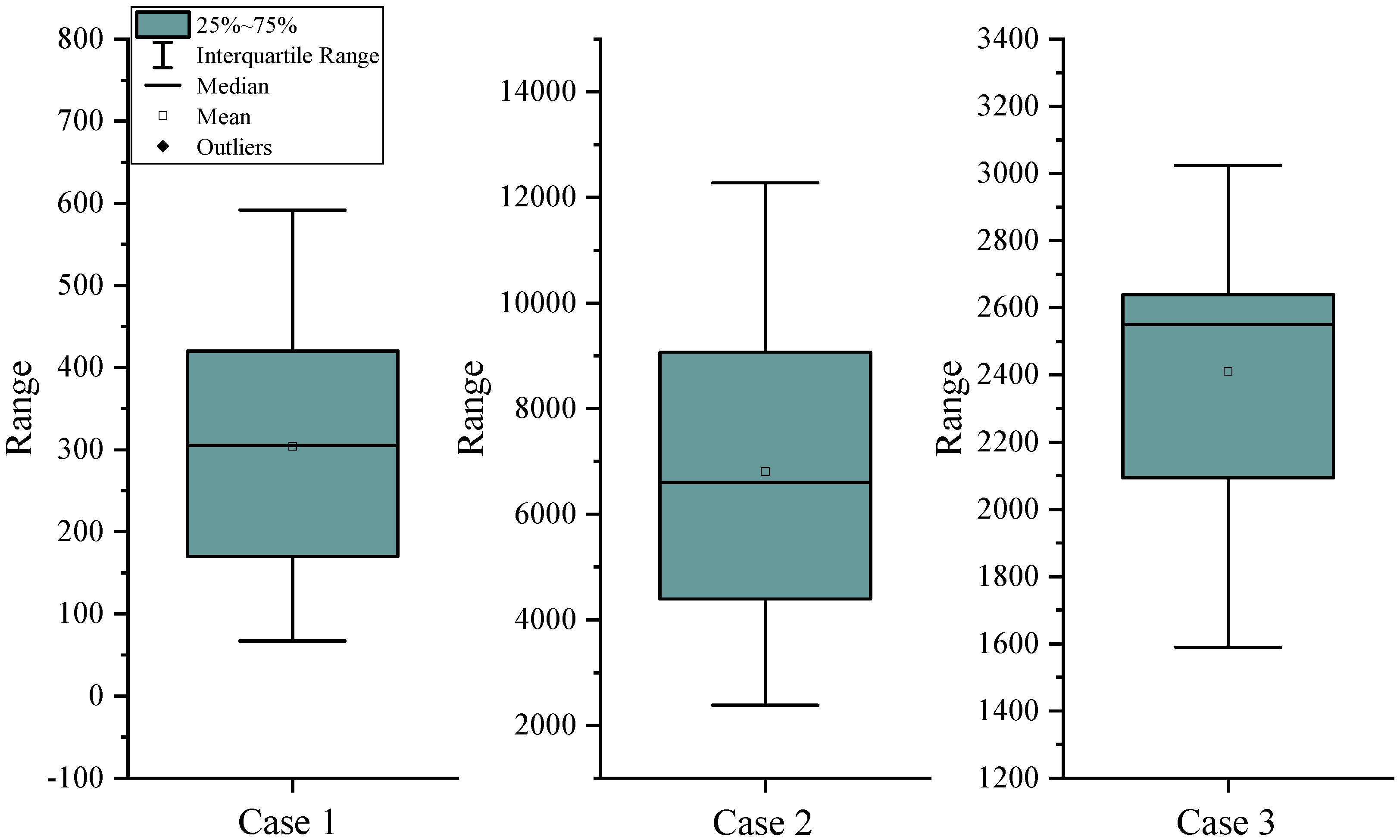
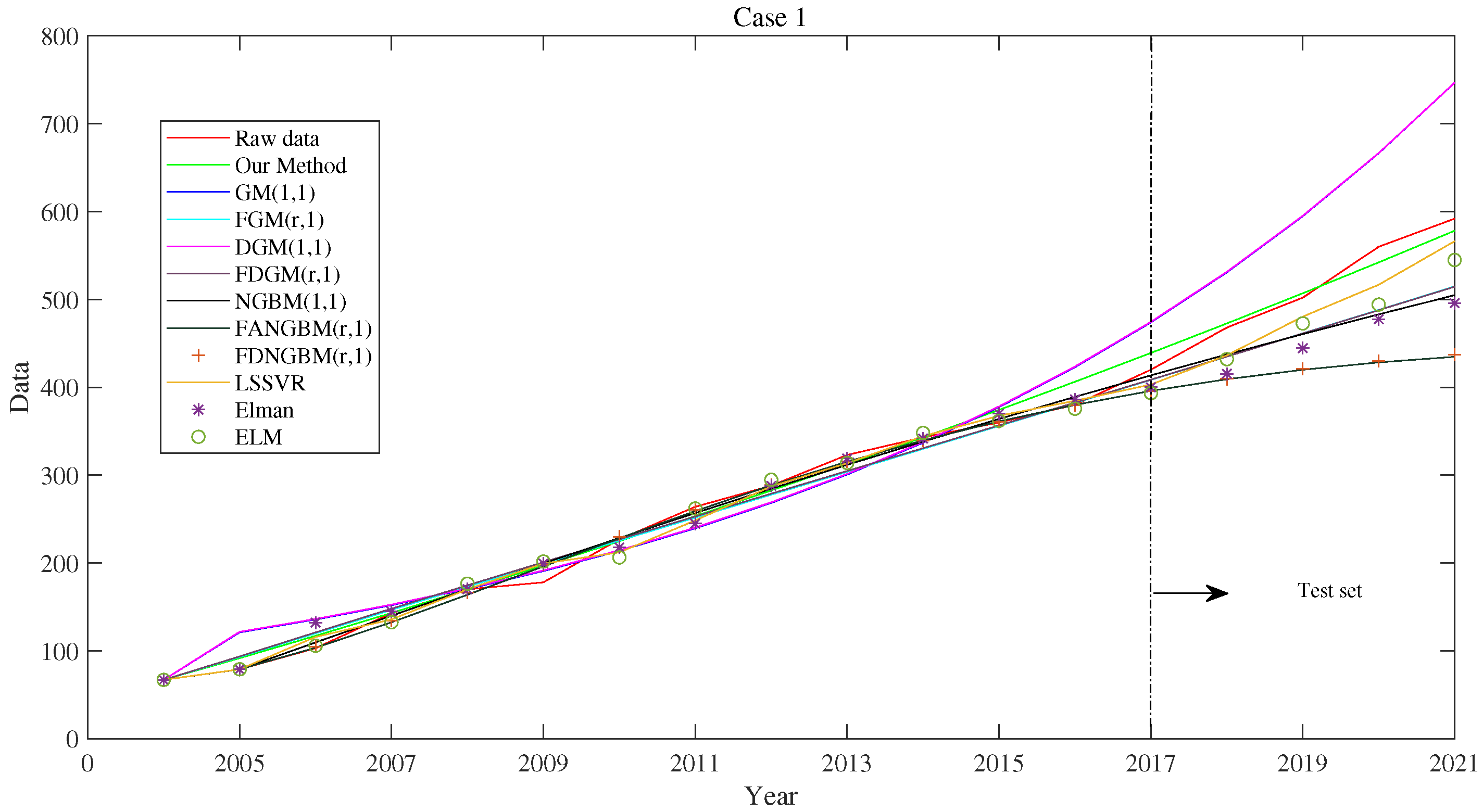
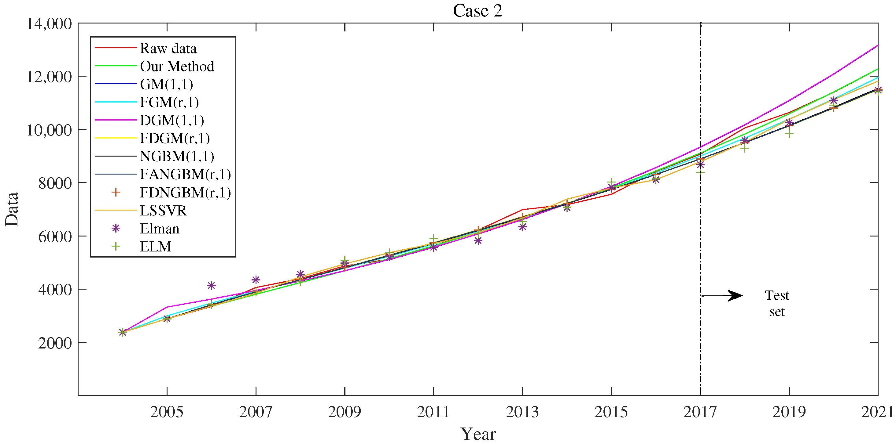
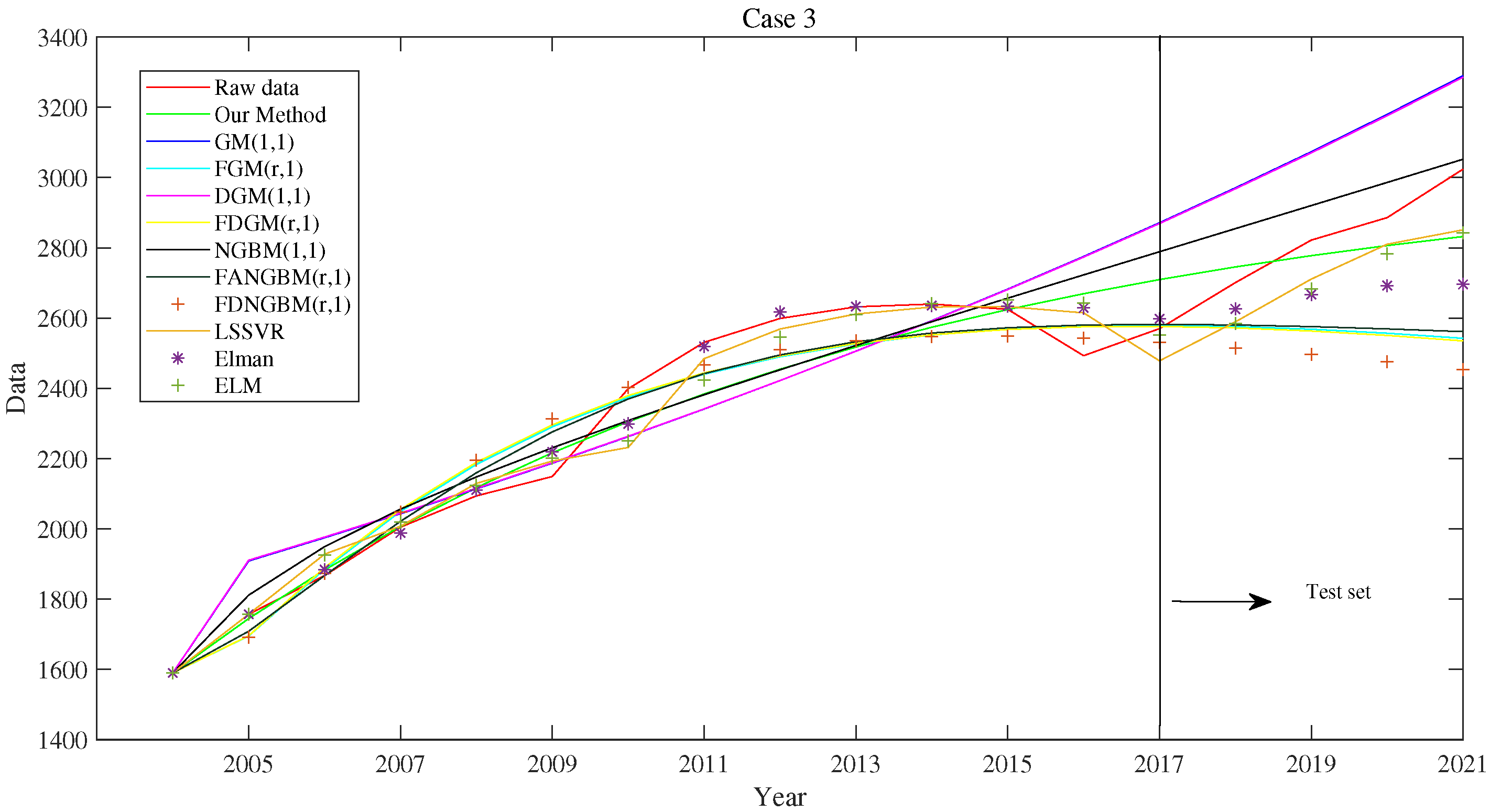
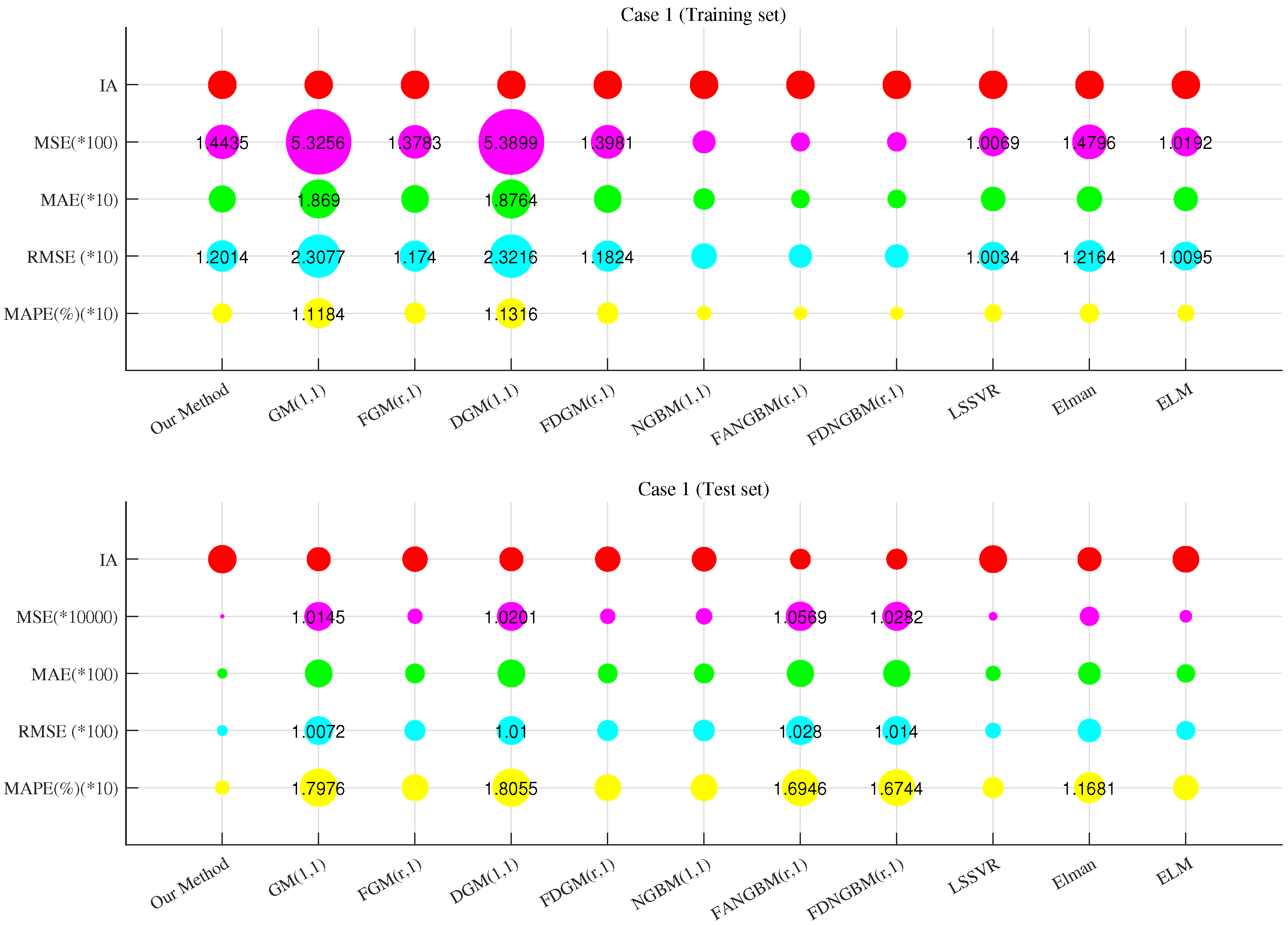
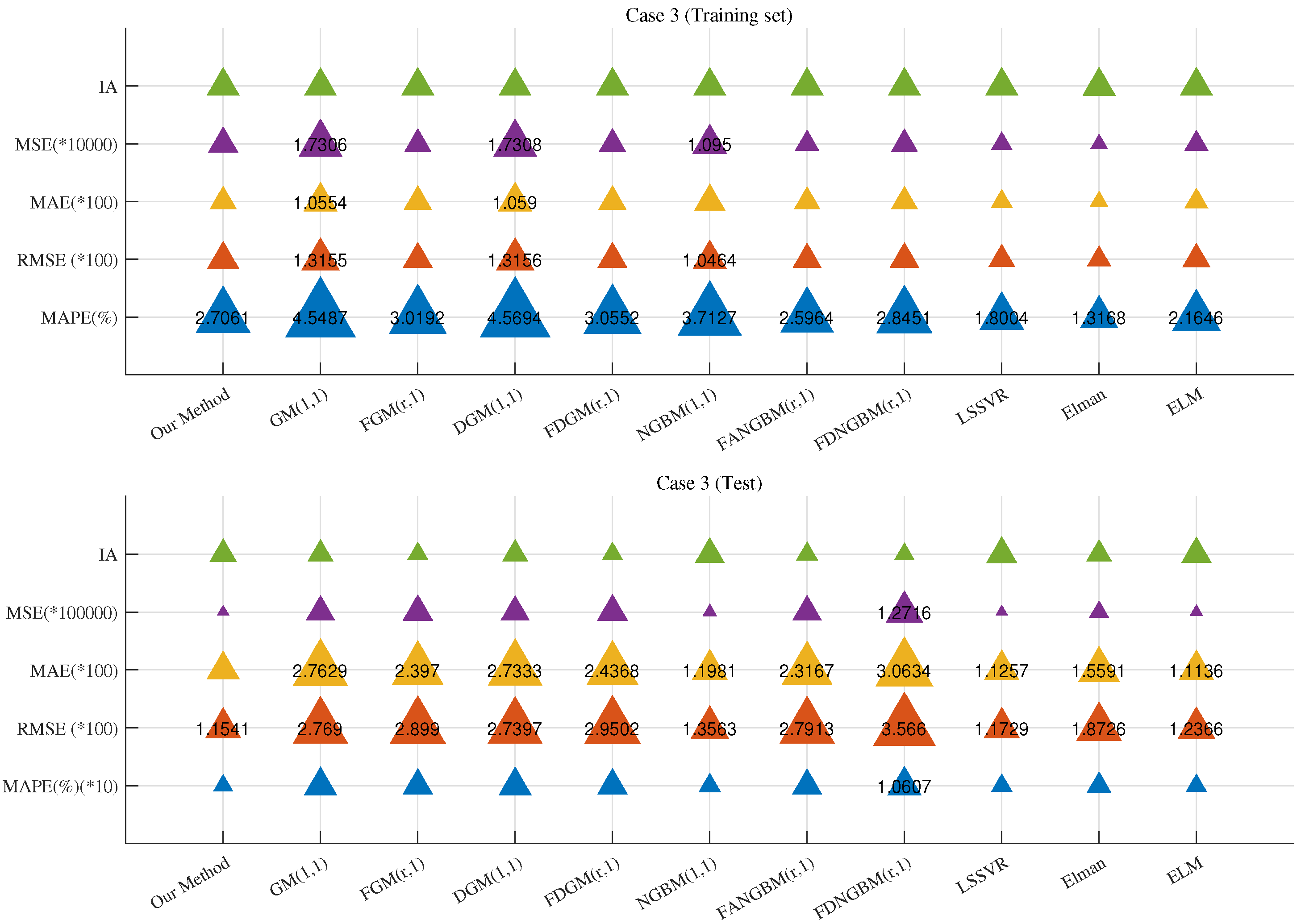
Based on the information shown in Figure 2, it can be understood that there are no outliers in the three datasets used, so they can be used directly for modeling. The modeling details of the proposed model are shown in Table 1, where r denotes the fractional-order parameter and a and b are the structural parameters. The models’ performance on the test sets in the cases is shown in Table 2, Table 3 and Table 4. The fitting curves of the models in the three cases are shown in Figure 3, Figure 4 and Figure 5. The results from Table 2, Table 3 and Table 4 are summarized in Figure 6, Figure 7 and Figure 8.
From Figure 6, Figure 7 and Figure 8, it can be visually observed that the proposed method corresponds to the lowest MAPE(test), RMSE(test), MAE(test), and MSE(test) among all the models. The statistical test results from Table 2, Table 3 and Table 4 also demonstrate significant differences between the proposed method and most competing models. Furthermore, based on Figure 3, Figure 4 and Figure 5, it can be seen that the green curve representing the proposed model closely aligns with the curve formed by the actual values in the test set for each case. Although the training set performance of the proposed method is not the best among the three cases, it ranks high in each case.
In all three cases, the proposed method performs better than the FGM(r,1) model, which confirms the motivation of this paper. Among the three original models (GM(1,1), DGM(1,1), and NGBM(1,1)), the overall performance of the fractional-order forms of the GM and DGM models outperforms the two original models, which is the reason why we optimized the fractional GM(1,1) model. Although the fractional-order model of NGBM(1,1) has better fitting performance than the NGBM(1,1) model, its test set performance is lower than NGBM(1,1) in three cases. This phenomenon is mainly caused by overfitting. The NGBM(1,1) model has a more complex modeling mechanism than the GM(1,1) model and the DGM(1,1) model, which makes it easily overfit. This is also the reason why the FGM(r,1) model was chosen for optimization instead of the FANGBM(r,1) model. In addition, it can be observed that the differences between the discrete models and the original models are very small. Compared with the original model, the discrete model is unbiased. Therefore, the discrete model may be more suitable for developing a new model. In general, the proposed method is superior to the GM(1,1) model and all its derived models, which verifies its validity.

3.3. Ablation Experiment

In this section, we will further verify the effectiveness of the proposed method by comparing its performance with that of its ablation models. The ablation models of the model in this paper include the GM(1,1) model, FGM(r,1) model, and model 1. Model 1 is a GM(1,1) model with structural parameters a and b obtained by the MPA. The performance of the proposed method and its ablation models in the three cases is shown in Table 5.
As can be seen from Table 5, in the three cases, the training set performance and test set performance of model 1 are better than those of the GM(1,1) model, and the training set performance and test set performance of the proposed model are better than those of the FGM(r,1) model, both of which indicate that the use of the optimization algorithm to obtain the structural parameters of the model directly is more effective than the traditional method. The proposed model outperforms model 1, and the FGM(r,1) model outperforms GM(1,1), both of which explain why the fractional-order model was chosen for optimization. In general, the optimized model outperforms all its ablation models in the training sets and test sets of the three cases, which verifies its effectiveness.

4. Conclusions

In this manuscript, we innovatively proposed a new method for obtaining the structural parameters of the fractional grey prediction model and validated the effectiveness of this method through cases. Compared to the structural parameters obtained through traditional parameter-estimation methods, the method proposed in this paper can obtain more flexible structural parameters. Not only that, this method also avoids potential overfitting issues that may exist during the parameter estimation process. What is even more noteworthy is that this method is applicable for optimizing any grey prediction model, a capability that many optimization measures lack.
Although the effectiveness of the method in this paper was verified, there are still some areas that can be improved. On the one hand, the experimental analysis showed that the discrete model is more suitable for developing the new model. On the other hand, there is no evidence to suggest that the marine predators algorithm is the most suitable algorithm for this model. In the future, we will continue to work to solve these problems.

Author Contributions

Y.W. contributed to the conception of the study and helped perform the analysis with constructive discussions. C.L. contributed to the analysis and manuscript preparation. Writing—original draft preparation, Y.W.; writing—review and editing, C.L. All authors have read and agreed to the published version of the manuscript.

Funding

This work was supported by the Guangdong Province Philosophy and Social Science Planning Project (Grant No. GD23YGL24).

Data Availability Statement

The data used to support the findings of this study are available from the corresponding author upon request.

Conflicts of Interest

The authors declare that they have no conflicts of interest.

References

  1. Ju-Long, D. Control problems of grey systems. Syst. Control Lett. 1982, 1, 288–294. [Google Scholar] [CrossRef]
  2. Şahin, U.; Şahin, T. Forecasting the cumulative number of confirmed cases of COVID-19 in Italy, UK and USA using fractional nonlinear grey Bernoulli model. Chaos Solitons Fractals 2020, 138, 109948. [Google Scholar] [CrossRef] [PubMed]
  3. Javed, S.A.; Zhu, B.; Liu, S. Forecast of biofuel production and consumption in top CO2 emitting countries using a novel grey model. J. Clean. Prod. 2020, 276, 123997. [Google Scholar] [CrossRef]
  4. Ding, S.; Hu, J.; Lin, Q. Accurate forecasts and comparative analysis of Chinese CO2 emissions using a superior time-delay grey model. Energy Econ. 2023, 126, 107013. [Google Scholar] [CrossRef]
  5. Sapnken, F.E.; Noume, H.C.; Tamba, J.G. Forecasting CO2 emissions from road fuel combustion using grey prediction models: A novel approach. MethodsX 2023, 11, 102271. [Google Scholar] [CrossRef] [PubMed]
  6. Liu, C.; Zhu, H.; Ren, Y.; Wang, Z. A Novel Intelligent Forecasting Framework for Quarterly or Monthly Energy Consumption. IEEE Trans. Ind. Inform. 2023, 20, 5352–5363. [Google Scholar] [CrossRef]
  7. Zhu, H.; Chong, L.; Wu, W.; Xie, W. A novel conformable fractional nonlinear grey multivariable prediction model with marine predator algorithm for time series prediction. Comput. Ind. Eng. 2023, 180, 109278. [Google Scholar] [CrossRef]
  8. Liu, C.; Wu, W.Z.; Xie, W. A new grey intelligent prediction algorithm with multiobjective correction strategy. Appl. Math. Model. 2023, 118, 692–708. [Google Scholar] [CrossRef]
  9. Liu, C.; Lao, T.; Wu, W.Z.; Xie, W.; Zhu, H. An optimized nonlinear grey Bernoulli prediction model and its application in natural gas production. Expert Syst. Appl. 2022, 194, 116448. [Google Scholar] [CrossRef]
  10. He, J.; Mao, S.; Ng, A.K. Neural computing for grey Richards differential equation to forecast traffic parameters with various time granularity. Neurocomputing 2023, 549, 126394. [Google Scholar] [CrossRef]
  11. Wu, L.; Liu, S.; Fang, Z.; Xu, H. Properties of the GM(1,1) with fractional order accumulation. Appl. Math. Comput. 2015, 252, 287–293. [Google Scholar] [CrossRef]
  12. Zhu, H.; Liu, C.; Wu, W.Z.; Xie, W.; Lao, T. Weakened fractional-order accumulation operator for ill-conditioned discrete grey system models. Appl. Math. Model. 2022, 111, 349–362. [Google Scholar] [CrossRef]
  13. Zhou, D. Least absolute deviation for parameter estimation of direct discrete GM(1,1) model. Stat. Decis. 2016, 2, 15–18. [Google Scholar]
  14. Luo, D.; Wei, B. A unified treatment approach for a class of discrete grey forecasting models and its application. Syst. Eng. Theory Pract. 2019, 39, 451–462. [Google Scholar]
  15. Wei, B.; Xie, N. Parameter estimation for grey system models: A nonlinear least squares perspective. Commun. Nonlinear Sci. Numer. Simul. 2021, 95, 105653. [Google Scholar] [CrossRef]
  16. Pei, L.; Li, Q.; Wang, Z. The NLS-based nonlinear grey Bernoulli model with an application to employee demand prediction of high-tech enterprises in China. Grey Syst. Theory Appl. 2018, 12, 133–143. [Google Scholar] [CrossRef]
  17. Zeng, B.; Liu, S. A self-adaptive intelligence gray prediction model with the optimal fractional order accumulating operator and its application. Math. Methods Appl. Sci. 2017, 40, 7843–7857. [Google Scholar] [CrossRef]
  18. Saxena, A. Optimized Fractional Overhead Power Term Polynomial Grey Model (OFOPGM) for market clearing price prediction. Electr. Power Syst. Res. 2023, 214, 108800. [Google Scholar] [CrossRef]
  19. Li, M.W.; Xu, R.Z.; Yang, Z.Y.; Hong, W.C.; An, X.G.; Yeh, Y.H. Optimization approach of berth-quay crane-truck allocation by the tide, environment and uncertainty factors based on chaos quantum adaptive seagull optimization algorithm. Appl. Soft Comput. 2024, 152, 111197. [Google Scholar] [CrossRef]
  20. Faramarzi, A.; Heidarinejad, M.; Mirjalili, S.; Gandomi, A.H. Marine Predators Algorithm: A nature-inspired metaheuristic. Expert Syst. Appl. 2020, 152, 113377. [Google Scholar] [CrossRef]
  21. Xie, N.; Liu, S. Discrete grey forecasting model and its optimization. Appl. Math. Model. 2009, 33, 1173–1186. [Google Scholar] [CrossRef]
  22. Wu, L.; Liu, S.; Yao, L. Discrete grey model based on fractional order accumulate. Syst. Eng. Theory Pract. 2014, 34, 1822–1827. [Google Scholar]
  23. Chen, C.I. Application of the novel nonlinear grey Bernoulli model for forecasting unemployment rate. Chaos Solitons Fractals 2008, 37, 278–287. [Google Scholar] [CrossRef]
  24. Şahin, U. Forecasting share of renewables in primary energy consumption and CO2 emissions of China and the United States under COVID-19 pandemic using a novel fractional nonlinear grey model. Expert Syst. Appl. 2022, 209, 118429. [Google Scholar] [CrossRef]
  25. Suykens, J.; Vandewalle, J.; De Moor, B. Optimal control by least squares support vector machines. Neural Netw. 2001, 14, 23–35. [Google Scholar] [CrossRef] [PubMed]
  26. Huang, G.B.; Zhu, Q.Y.; Siew, C.K. Extreme learning machine: A new learning scheme of feedforward neural networks. In Proceedings of the 2004 IEEE International Joint Conference on Neural Networks (IEEE Cat. No.04CH37541), Budapest, Hungary, 25–29 July 2004; Volume 2, pp. 985–990. [Google Scholar] [CrossRef]
  27. Elman, J.L. Finding Structure in Time. Cogn. Sci. 1990, 14, 179–211. [Google Scholar] [CrossRef]
  28. Diebold, F.X.; Mariano, R.S. Comparing Predictive Accuracy. J. Bus. Econ. Stat. 2002, 20, 134–144. [Google Scholar] [CrossRef]
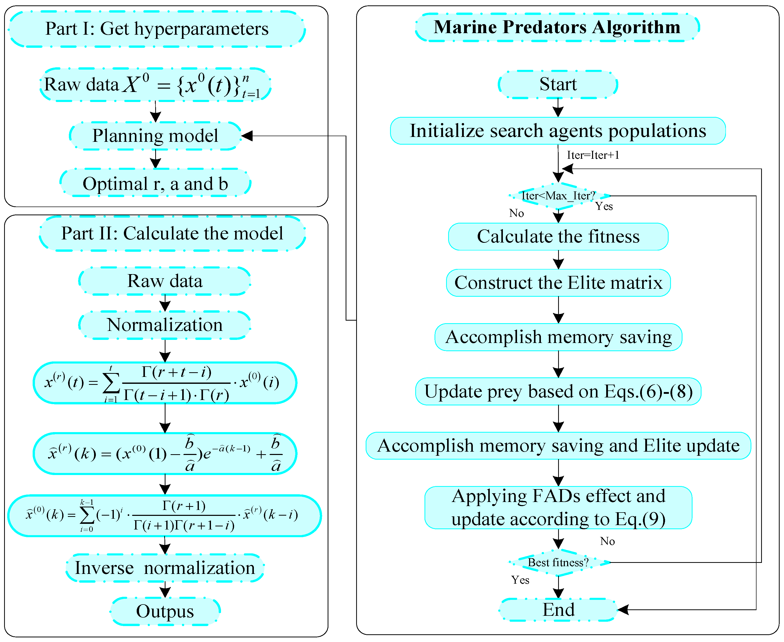
Figure 1. The operational process of the proposed method.
Fractalfract 08 00396 g001
Figure 2. Outlier detection based on the boxplot.
Fractalfract 08 00396 g002
Figure 3. The fitting curves of the models in case 1.
Fractalfract 08 00396 g003
Figure 4. The fitting curves of the models in case 2.
Fractalfract 08 00396 g004
Figure 5. The fitting curves of the models in case 3.
Fractalfract 08 00396 g005
Figure 6. The evaluation metrics of the models in case 1.
Fractalfract 08 00396 g006
Figure 7. The evaluation metrics of the models in case 2.
Fractalfract 08 00396 g007
Figure 8. The evaluation metrics of the models in case 3.
Fractalfract 08 00396 g008
Table 1. Hyperparameters of the proposed model for the three cases.
Caserab
10.0114−0.02390.062
20.7867−0.06910.2532
30.00030.11230.1298
Table 2. Performance of methods in case 1.
IndexTraining set
Our methodGM(1,1) ***FGM(r,1)DGM(1,1) ***FDGM(r,1)NGBM(1,1) *FANGBM(r,1) *FDNGBM(r,1) *LSSVRElmanELM
MAPE4.746211.18385.464311.31585.63962.58622.14032.15403.76634.55903.4771
RMSE12.014423.077311.740023.216211.82427.98896.63136.759710.034212.164010.0955
MAE8.887818.68989.377318.76369.37565.56964.14904.16917.37217.91187.1557
MSE144.3457532.5610137.8273538.9924139.811863.822243.974245.6936100.6859147.9637101.9184
IA0.99680.98750.99670.98740.99660.99850.99900.99900.99770.99660.9977
IndexTest set
Our methodGM(1,1) ***FGM(r,1) ***DGM(1,1) ***FDGM(r,1) ***NGBM(1,1) **FANGBM(r,1) ***FDNGBM(r,1) ***LSSVR **Elman ***ELM ***
MAPE2.410717.97638.758718.05488.76728.956316.945516.74375.427711.68057.9137
RMSE13.5587100.722952.9336100.997553.086356.9316102.8033101.401429.261367.100143.3794
MAE12.076494.133246.873994.502546.941548.507790.780389.662127.805961.724240.9576
MSE183.838110,145.09832801.966910,200.50192818.15373241.208710,568.508410,282.2380856.22414502.41741881.7688
IA0.98510.71060.78310.70920.78140.74040.52360.53010.94290.70950.8755
* implies that the result of the statistical test is significant at a confidence level of 90 % . ** means that the result of the statistical test is significant at a confidence level of 95 % . *** means that the result of the statistical test is significant at a confidence level of 99 % . Note that the loss function used in this paper for the DM test is the absolute value of the error.
Table 3. Performance of methods in case 2.
IndexTraining set
Our methodGM(1,1)FGM(r,1)DGM(1,1)FDGM(r,1)NGBM(1,1)FANGBM(r,1)FDNGBM(r,1)LSSVRElman *ELM **
MAPE1.89033.60292.02143.58891.66931.65881.64881.62922.39294.88083.2101
RMSE151.7300213.5728130.0677213.9911124.4167123.9353124.0086123.2995181.7177339.1109238.7100
MAE104.2117165.2994102.8817164.699594.996093.757993.511292.2995144.7706246.8396191.3288
MSE23,021.981845,613.340016,917.603345,792.182715,479.507215,359.959115,378.137815,202.763433,021.3086114,996.176556,982.4602
IA0.99830.99650.99870.99650.99880.99880.99880.99880.99750.99040.9956
IndexTest set
Our methodGM(1,1) **FGM(r,1) ***DGM(1,1) **FDGM(r,1) ***NGBM(1,1) ***FANGBM(r,1) ***FDNGBM(r,1) ***LSSVR ***Elman **ELM ***
MAPE0.65274.26482.34904.36614.76664.57044.72764.75163.40014.39106.7996
RMSE106.6044551.5302276.4134561.3699560.0621532.7855553.3528555.5588379.3698504.1814732.7698
MAE65.5743476.0711255.1534486.8833523.5790500.8322518.7340521.2318361.6793473.7329720.6889
MSE11,364.5080304,185.558276,404.3905315,136.1645313,669.5868283,860.4294306,199.3710308,645.5360143,921.4154254,198.8576536,951.6334
IA0.99770.95140.98360.94970.92770.93540.92980.92930.97050.94530.8985
* implies that the result of the statistical test is significant at a confidence level of 90 % . ** means that the result of the statistical test is significant at a confidence level of 95 % . *** means that the result of the statistical test is significant at a confidence level of 99 % .
Table 4. Performance of methods in case 3.
IndexTraining set
Our methodGM(1,1) **FGM(1,1)DGM(1,1) **FDGM(1,1)NGBM(1,1) *FANGBM(1,1)FDNGBM(r,1)LSSVRElman **ELM
MAPE2.70614.54873.01924.56943.05523.71272.59642.84511.80041.31682.1646
RMSE90.0727131.552280.4085131.559581.0309104.640073.198379.403064.113551.702872.0018
MAE66.5238105.544170.3071105.898870.853087.061761.631665.739841.986830.781951.1383
MSE8113.086117,305.98296465.525317,307.89746566.008010,949.53815357.98566304.83714110.54292673.18285184.2656
IA0.98270.96120.98610.96110.98580.97610.98860.98650.99160.99480.9894
IndexTest set
Our methodGM(1,1) ***FGM(1,1) *DGM(1,1) ***FDGM(1,1) *NGBM(1,1)FANGBM(1,1) *FDNGBM(r,1) **LSSVRElmanELM
MAPE3.55109.91338.26029.80918.39624.41737.987510.60743.99465.38263.8931
RMSE115.4096276.9010289.9036273.9747295.0238135.6279279.1346356.5978117.2942187.2595123.6559
MAE99.9885276.2853239.6955273.3341243.6816119.8090231.6709306.3397112.5747155.9057111.3554
MSE13,319.382076,674.143484,044.077775,062.158687,039.050518,394.919077,916.1112127,161.996813,757.934035,066.136915,290.7848
IA0.67130.60610.41140.60910.40640.77080.42600.36320.86210.59350.8218
* implies that the result of the statistical test is significant at a confidence level of 90 % . ** means that the result of the statistical test is significant at a confidence level of 95 % . *** means that the result of the statistical test is significant at a confidence level of 99 % .
Table 5. The performance of the proposed method and its ablation models in the three cases.
Training setOur methodGM(1,1)FGM(1,1)Model 1Our methodGM(1,1)FGM(1,1)Model 1Our methodGM(1,1)FGM(1,1)Model 1
Case 1Case 2Case 3
MAPE4.746211.18385.464310.36411.89033.60292.02143.45372.70614.54873.01924.3680
RMSE12.014423.077311.740024.1802151.7300213.5728130.0677226.507890.0727131.552280.4085137.8683
MAE8.887818.68989.377319.4523104.2117165.2994102.8817144.681666.5238105.544170.3071104.1649
MSE144.3457532.5610137.8273584.681323,021.981845,613.340016,917.603351,305.78378113.086117,305.98296465.525319,007.6761
IA0.99680.98750.99670.98570.99830.99650.99870.99590.98270.96120.98610.9559
Test setOur methodGM(1,1)FGM(1,1)Model 1Our methodGM(1,1)FGM(1,1)Model 1Our methodGM(1,1)FGM(1,1)Model 1
MAPE2.410717.97638.758713.95370.65274.26482.34902.19923.55109.91338.26027.3533
RMSE13.5587100.722952.933681.7926106.6044551.5302276.4134289.0112115.4096276.9010289.9036205.5850
MAE12.076494.133246.873973.888865.5743476.0711255.1534246.502499.9885276.2853239.6955204.4749
MSE183.838110,145.09832801.96696690.037211,364.5080304,185.558276,404.390583,527.492713,319.382076,674.143484,044.077742,265.1836
IA0.98510.71060.78310.78180.99770.95140.98360.98510.67130.60610.41140.6968
Disclaimer/Publisher’s Note: The statements, opinions and data contained in all publications are solely those of the individual author(s) and contributor(s) and not of MDPI and/or the editor(s). MDPI and/or the editor(s) disclaim responsibility for any injury to people or property resulting from any ideas, methods, instructions or products referred to in the content.