Multi-Point Seawall Settlement Prediction with Limited Data Volume Using an Improved Fractional-Order Grey Model

Abstract

Settlement prediction based on monitoring data holds significant importance for engineering maintenance of seawalls. In practical engineering, the volume of the collected monitoring data is often limited due to the restrictions of devices and engineering budgets. Previous studies have applied the fractional-order grey model to time series prediction under the situation of limited data volume. However, the performance of the fractional-order grey model is easily affected by the inappropriate settings of fractional order. Also, the model cannot make dynamic predictions due to the characteristic of fixed step size. To solve the above problems, in this paper, the genetic algorithm with enhanced search capabilities was employed to solve the premature convergence problem. Additionally, to solve the problem of the fractional-order grey model associated with fixed step size, the real-time tracing algorithm was introduced to conduct equal-dimensionally recursive calculation. The proposed model was validated using monitoring data of four monitoring points at Haiyan seawall in Zhejiang province, China. The prediction performance of the proposed model was then compared with those of the fractional-order GM(1,1), integer-order GM(1,1), and fractal theory model. Results indicate that the proposed model significantly improves the prediction performance compared to other models.

1. Introduction

Seawalls are commonly established atop foundations of deep soft soils whose physical and mechanical features are distinctive, e.g., high compressibility, high water content, and diminished strength, as well as specific rheological behavior [1,2]. These characteristics lead to significant settlement during both the construction phase and post-construction phase. The total subsidence may reach several meters and the consolidation settlement period lasts more than 10 years [3,4,5]. The large vertical settlement on soft soil foundations threatens the stability of seawalls, which greatly increases the risk of structural damage and safety incidents. Therefore, predicting seawall settlement is essential to engineering security operations and risk management.

Time series monitoring data record the historical behavior of seawalls, including its structural characteristics and operational patterns [6,7] among which settlement is one of the most crucial parameters. Predicting the settlement based on time series monitoring data using mathematical algorithms forms a reliable approach for assessing the safety status of the seawall [8,9]. At present, prediction methods commonly used in seawall settlement prediction based on monitoring data can be categorized into two groups: statistical methods and machine learning methods. Statistical methods such as the exponential curve method [10], Asaoka method [11], and Poisson curve method [12] are established based on the idea of data fitting using mathematical curves. Statistical models can not only quantify the influence of each factor on data-varying tendencies, but also effectively describe the characteristics of the data sequence including the distribution and correlation of data. These models are usually established on the basis of certain assumptions such as normality, independence, etc., which means that the accuracy and reliability of the model cannot be guaranteed in the case where the assumptions are not met [13,14]. Machine learning methods, such as wavelet theory [15], chaos theory [16], and neural networks [17], are able to process massive and multidimensional datasets to solve nonlinear and complicated problems. However, both statistical methods and machine learning methods are highly reliant on the quantity and quality of data sequences, meaning that either poor data quality or insufficient data quantity can lead to unsatisfactory prediction performance [15,18].

Insufficient data volume is a common issue in seawall settlement monitoring. In many cases, the volume of monitoring data is fairly limited, and this is not an isolated occurrence [19,20]. The reasons are multifaceted; the number of monitoring devices installed on the seawall may be insufficient to cover all critical areas, resulting in limited data availability. Even with adequate monitoring devices, the current technology may not support high-density and high-precision monitoring, thereby restricting the monitoring frequency and causing a shortage in data volume [21]. Further, due to the intricate environmental conditions in coastal areas, environmental factors during critical periods such as storm surges and floods can further impede the acquisition of monitoring data. The insufficient amount of data in seawall monitoring is a significant issue as it may limit our comprehensive evaluation of a seawall’s health condition and potential risks [22,23]. This issue can be addressed in two aspects to ensure the accurate prediction of a seawall’s settlement based on monitoring data. We can either increase the number of monitoring points or strengthen the ability of data processing and analysis under the situation of limited data volume.

Most previous studies developed predictive models using monitoring data at a single monitoring point. Using multi-point monitoring data prediction offers several advantages over single-point data prediction, particularly in terms of robustness and ability to capture complex relationships [24,25]. First, multi-point monitoring data provides multiple observations of the same phenomenon, reducing the impact of errors or noise from any single point. Also, different data points can capture various aspects of the system, leading to a more comprehensive understanding and improved prediction accuracy. It allows the prediction model to be less sensitive to missing or erroneous data from individual sensors. Therefore, multi-point prediction provides a solution to ensure the efficiency and accuracy of seawall settlement displacement.

In addition, in engineering cases where a lack of monitoring data is already present, employing mathematical methods to analyze and predict the existing dataset emerges as the most practical, effective, and economical approach. Grey models, especially the GM(1,1) model, exhibit significant advantages in tackling issues related to insufficient data volume [26,27]. In the realm of grey theory, the grey system comprises known information (white) and unknown or uncertain information (grey or black). Grey models use limited and incomplete data to establish differential predictive models, thereby uncovering latent patterns within the dataset [28,29,30,31]. Their core competency lies in making predictions with relatively small amounts of data. Typically, only a few data points (four or more) are required to build a grey predictive model, effectively addressing the issues of scarce historical data, incomplete series, and low reliability. In addition, grey models do not require strict regularity in the distribution of sample data, further easing the data requirements.

While grey models possess these advantages, they also have limitations. For instance, they may not be optimal for systems with clearly defined internal mechanisms, and may fall into suboptimal solutions in predicting time series data with high volatility. Wu [32] found that the GM(1,1) model exhibits considerable sensitivity to minor perturbations in data computation using matrix perturbation theory, resulting in significant interference with the identification of model parameters. To address this issue, he proposed a fractional-order grey model on the basis of the perturbation theory of least squares [33]. The fractional-order grey model, as an extended grey prediction model, is exceptionally adept at handling data sequences that exhibit volatile variations. By introducing fractional-order calculus operators into a continuous grey model, it adeptly transforms original data sequences with fluctuations into ones with heightened regularity, thereby optimizing the traditional grey modeling mechanism and improving the modeling efficiency [34].

Although the fractional-order grey model exhibits advantages in handling complex systems, its application to the prediction of seawall settlement with limited data volume can still be constrained by system and data characteristics. As the fractional-order grey model incorporates fractional-order derivatives and polynomial functions, the determination of its parameters becomes more complex, requiring the employment of specific optimization methods to solve the coefficients of polynomial functions. For example, the variable fractional order r obtained by commonly used intelligent algorithms involves unavoidable randomness, which may increase the unitability of prediction results [35]. For example, the swarm optimization algorithm may obtain a local optimal solution instead of a global optimal solution due to its high convergence speed [36]. The artificial fish swarm algorithm is susceptible to premature convergence, that is, the algorithm may converge to a suboptimal solution without adequately exploring the searching space [37]. Further, the fractional-order grey model cannot fit the time series data dynamically. Due to the high sensitivity and compressibility characteristics of the soft soil foundation of the seawall, and influenced by external factors such as tidal scouring, storm surges, and construction disturbances, the settlement of the seawall exhibits dynamic variations at small temporal scales [38]. Seawall settlement represents a real-time evolving process, but the fractional-order grey model is limited to making predictions with a fixed step size based on existing data [8,39]; therefore, the dynamic prediction of seawall settlement still needs to be improved.

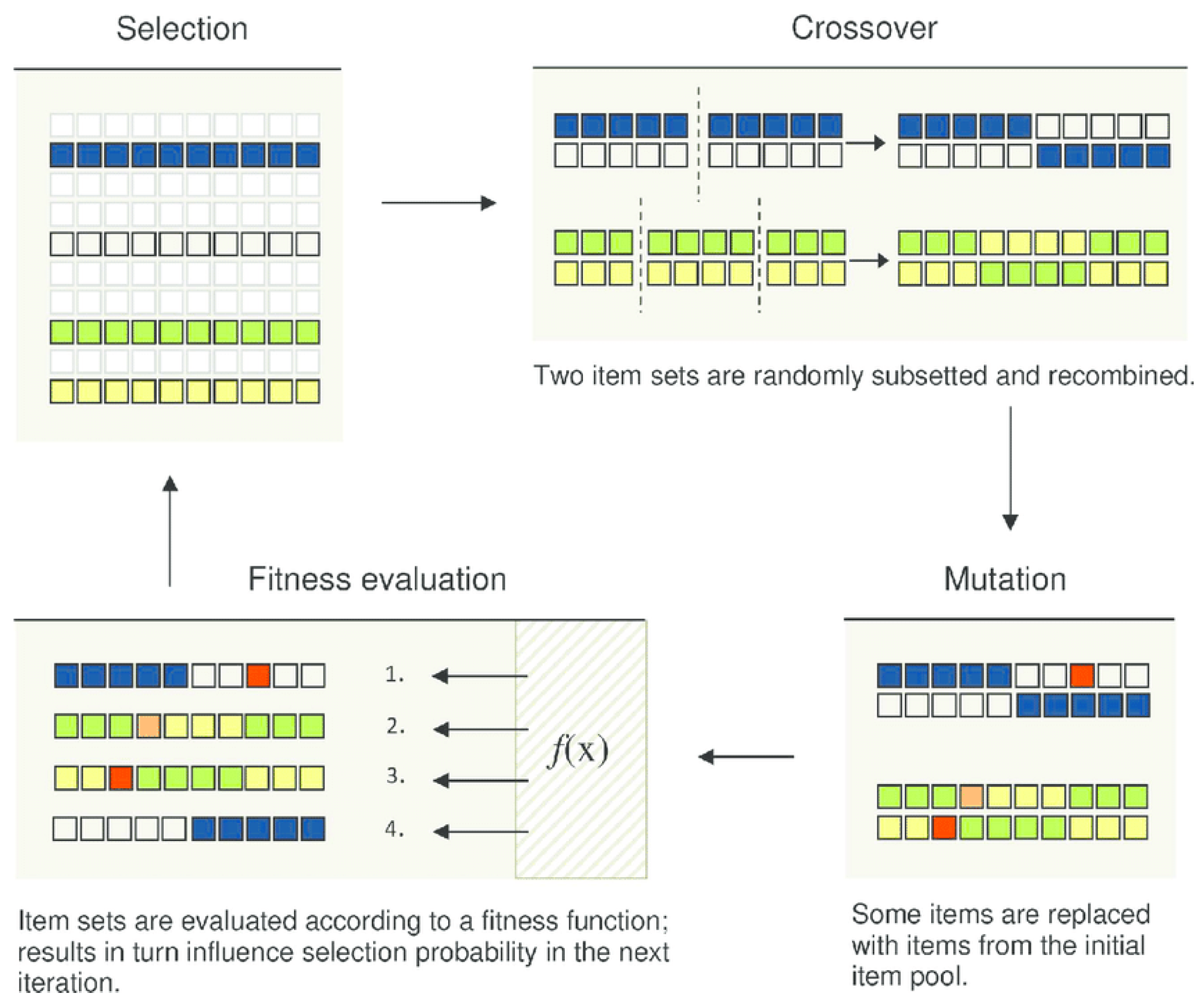
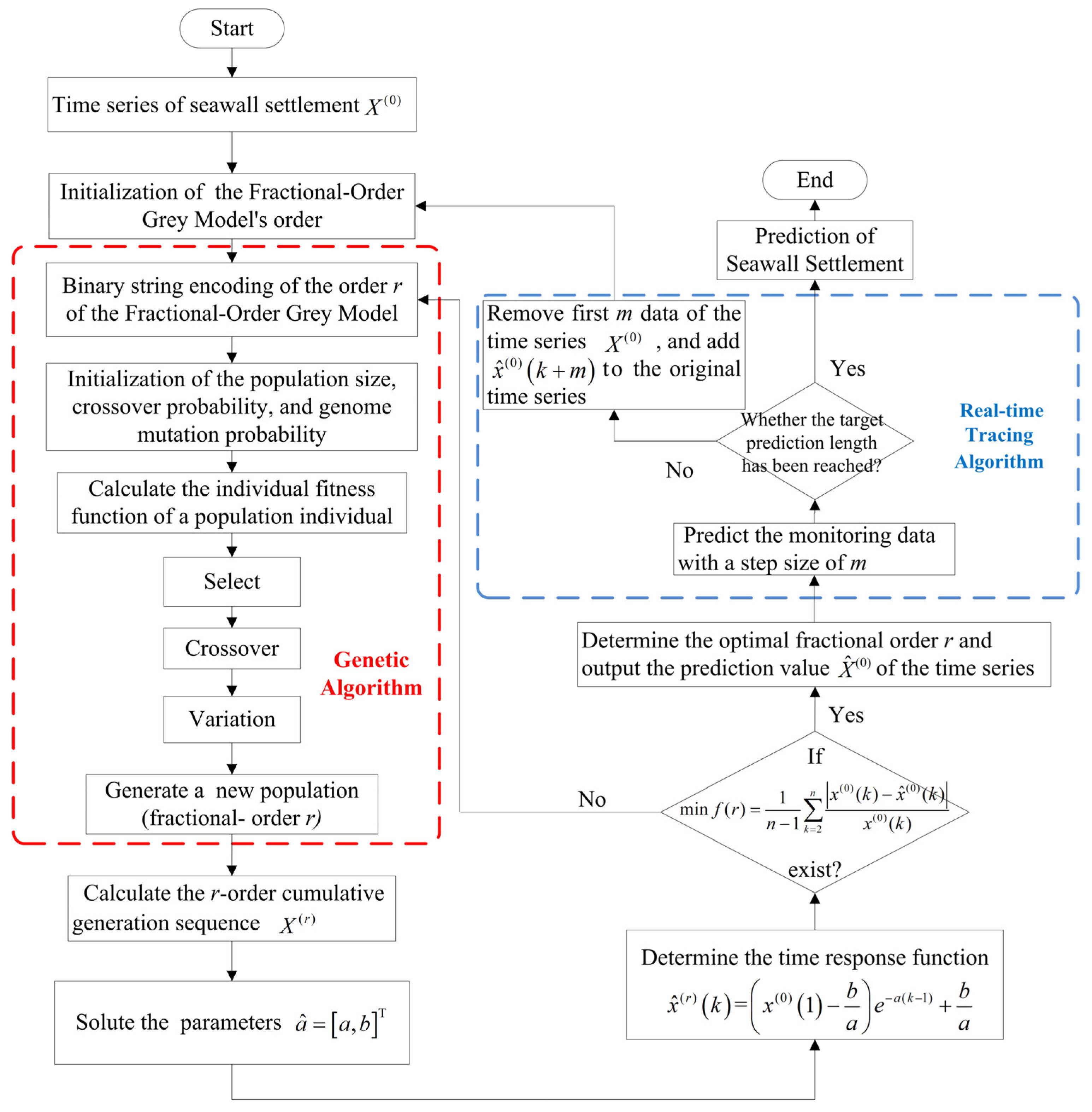
To solve the above two issues associated with the application of the fractional-order grey model in seawall settlement prediction in the case of limited data volume, this study aims to improve the fractional-order grey model by integrating other models. With this objective in mind, a genetic algorithm [40] with enhanced search capabilities was used to solve and optimize the fractional order r of the fractional-order grey model. Then, a real-time tracing algorithm [41] was used to achieve the dynamic prediction. The monitoring of the data of a seawall at the northern bank of the Qiantang River, China, was used to validate the model. The performance of the proposed model was evaluated by comparison with the fractional-order GM(1,1), integer-order GM(1,1), and fractal theory model, respectively.

This paper is organized as follows: Section 2 presents how the proposed model is developed. Section 3 exhibits the information of the case study. Section 4 shows the prediction results. Comparisons of the proposed model with other relative models are also illustrated in this section. Section 5 presents the concluding remarks.

2. Model Development

This section presents the principles of the proposed model including the definitions, modeling procedures, parameter settings, and implementation steps.

2.1. Establishment of the Fractional-Order Grey Model

The most commonly used grey model is the GM(1,1) model, which is an integer-order accumulated generating sequence. Compared to the GM(1,1) model, the fractional-order grey model exhibits greater robustness and has a better performance to cope with datasets with limited volume, and its principles include the following steps [42,43]:

Assuming that the sequence $X^{(0)}=\left(x^{\left(0\right)}\left(1\right),x^{\left(0\right)}\left(2\right),\cdots x^{\left(0\right)}\left(n\right)\right)$ is the original monitoring data and $r\in R^{+}$, then the r-order accumulated generating sequence of $X^{(0)}$ can be written as $X^{(r)}=\left(x^{(r)}\left(1\right),x^{(r)}\left(2\right),\cdots x^{(r)}\left(n\right)\right)$, where

$$x^{(r)}\left(k\right)={\displaystyle \sum _{i=1}^k\frac{\Gamma \left(r+k-i\right)}{\Gamma \left(k-i+1\right)\Gamma \left(r\right)}}{x}^{(0)}\left(i\right), k=1,2,\cdots ,n.$$

(1)

$\Gamma \left(r\right)$ represents the Gamma function of order r, which is defined as

$$\Gamma \left(r\right)={\displaystyle {\int }_0^{\infty }{e}^{-t}{t}^{r-1}}dt.$$

(2)

The r-order cumulative generating sequence of $X^{(0)}$ can be written as $X^{(-r)}=\left(x^{(-r)}\left(1\right),x^{(-r)}\left(2\right),\cdots x^{(-r)}\left(n\right)\right)$, where

$$x^{(-r)}\left(k\right)={\displaystyle \sum _{i=0}^{k-1}\frac{\Gamma \left(r+1\right)}{\Gamma \left(i+1\right)\Gamma \left(r-i+1\right)}}{x}^{(0)}\left(k-i\right), k=1,2,\cdots ,n$$

(3)

Then the first-order cumulative generating sequence of $X^{(r)}$ can be written as $X^{(r-1)}=\left(x^{(r-1)}\left(1\right),x^{(r-1)}\left(2\right),\cdots x^{(r-1)}\left(n\right)\right)$, where

$$x^{(r-1)}\left(k\right)={(x^{(r)})}^{(-1)}\left(k\right)=x^{(r)}\left(k\right)-x^{(r)}\left(k-1\right), k=2,3,\cdots ,n$$

(4)

The sequence $Z^{(r)}=\left(z^{(r)}\left(2\right),z^{(r)}\left(3\right),\cdots z^{(r)}\left(n\right)\right)$ can be generated by the close mean value of the r-order accumulated generating sequence $X^{(r)}$, where

$$z^{(r)}\left(k\right)={\displaystyle \frac{x^{(r)}\left(k\right)+x^{(r)}\left(k-1\right)}{2}}, k=2,3,\cdots ,n$$

(5)

Then, the proposed model of the monitoring data is

$$x^{(r-1)}\left(k\right)+a{z}^{(r)}=b$$

(6)

The parameter $\widehat{a}={\left[a,b\right]}^{\mathrm{T}}$ can be estimated by the least square method:

$$\widehat{a}={\left(B^{\mathrm{T}}B\right)}^{-1}{B}^{\mathrm{T}}Y$$

(7)

where Y and B are

$$Y=\left[\begin{array}{l}{x}^{(r-1)}\left(2\right)\\ x^{(r-1)}\left(3\right)\\ ⋮\\ x^{(r-1)}\left(n\right)\end{array}\right], B=\left[\begin{array}{l}-z^{(r)}\left(2\right)-1\\ -z^{(r)}\left(3\right)-1\\ ⋮⋮\\ -z^{(r)}\left(n\right)-1\end{array}\right]$$

(8)

Since

$$\begin{array}{cc}\hfill x^{(r-1)}\left(k\right)& =x^{(r)}\left(k\right)-x^{(r)}\left(k-1\right)\hfill \\ & ={\displaystyle \sum _{i=1}^k\frac{\Gamma \left(r+k-i\right)}{\Gamma \left(k-i+1\right)\Gamma \left(r\right)}}{x}^{(0)}\left(i\right)-{\displaystyle \sum _{i=1}^{k-1}\frac{\Gamma \left(r+k-i-1\right)}{\Gamma \left(k-i\right)\Gamma (r)}}{x}^{(0)}\left(i\right), k=2,3,\cdots ,n\hfill \end{array}$$

(9)

then

$$z^{(r)}(k)={\displaystyle \frac{{\displaystyle \sum _{i=1}^k\frac{\Gamma \left(r+k-i\right)}{\Gamma \left(k-i+1\right)\Gamma \left(r\right)}}{x}^{(0)}\left(i\right)}{2}}+{\displaystyle \frac{{\displaystyle \sum _{i=1}^{k-1}\frac{\Gamma \left(r+k-i\right)}{\Gamma \left(k-i+1\right)\Gamma (r)}}{x}^{(0)}\left(i\right)}{2}}, k=2,3,\cdots ,n$$

(10)

Finally, Y and B can be obtained:

$$Y=\left[\begin{array}{c}(r-1)x^{(0)}(1)+x^{(0)}(2)\\ {\displaystyle \frac{r(r-1)}{2}}{x}^{(0)}(1)+(r-1)x^{(0)}(2)+x^{(0)}(3)+\cdots \\ ⋮\\ {\displaystyle \sum _{i=1}^n\frac{\Gamma \left(r+n-i\right)}{\Gamma \left(n-i+1\right)\Gamma (r)}}{x}^{(0)}\left(i\right)-{\displaystyle \sum _{i=1}^{n-1}\frac{\Gamma \left(r+n-i-1\right)}{\Gamma \left(n-i\right)\Gamma (r)}}{x}^{(0)}\left(i\right)\end{array}\right],$$

(11)

$$B=\left[\begin{array}{ll}-{\displaystyle \frac{x^{(r)}\left(1\right)+x^{(r)}\left(2\right)}{2}}& \hfill 1\\ -{\displaystyle \frac{x^{(r)}\left(2\right)+x^{(r)}\left(3\right)}{2}}& \hfill 1\\ \hfill ⋮\hfill & \hfill ⋮\\ -{\displaystyle \frac{x^{(r)}\left(n-1\right)+x^{(r)}\left(n\right)}{2}}& \hfill 1\end{array}\right]=\left[\begin{array}{ll}-{\displaystyle \frac{1}{2}}\left[(r+1)x^{(0)}\left(1\right)+x^{(0)}\left(2\right)\right]& \hfill 1\\ -{\displaystyle \frac{1}{2}}\left[{\displaystyle \frac{r(r+3)}{2}}{x}^{(0)}\left(1\right)+(r+1)x^{(0)}\left(2\right)+x^{(0)}\left(3\right)\right]& \hfill 1\\ \hfill ⋮\hfill & \hfill ⋮\\ -{\displaystyle \frac{1}{2}}\left[{\displaystyle \sum _{i=1}^n\frac{\Gamma \left(r+n-i\right)}{\Gamma \left(n-i+1\right)\Gamma (r)}}{x}^{(0)}\left(i\right)-{\displaystyle \sum _{i=1}^{n-1}\frac{\Gamma \left(r+n-i\right)}{\Gamma \left(n-i+1\right)\Gamma (r)}}{x}^{(0)}\left(i\right)\right]& \hfill 1\end{array}\right].$$

(12)

${\displaystyle \frac{d{x}^{(r)}}{dt}}+a{x}^{(r)}=b$ is the whitenization equation of the FGM $x^{(r-1)}\left(k\right)+a{z}^{(r)}=b$, and therefore the time response function is

$${\widehat{x}}^{(r)}\left(k\right)=\left(x^{(0)}\left(1\right)-{\displaystyle \frac{b}{a}}\right)e^{-a(k-1)}+{\displaystyle \frac{b}{a}}, k=2,3,\cdots ,n$$

(13)

Then, the restored monitoring data ${\widehat{X}}^{(0)}=\left({\widehat{x}}^{(0)}\left(1\right),{\widehat{x}}^{(0)}\left(2\right),\cdots {\widehat{x}}^{(0)}\left(k\right)\right)$ can be obtained, where ${\widehat{x}}^{(0)}\left(1\right)=x^{(0)}\left(1\right)$, and

$${\widehat{x}}^{(0)}\left(k\right)={\left({\widehat{x}}^{(r)}\right)}^{-r}\left(k\right)={\displaystyle \sum _{i=0}^{k-1}{(-1)}^i\frac{\Gamma \left(r+1\right)}{\Gamma \left(i+1\right)\Gamma \left(r-i+1\right)}}{\widehat{x}}^{(r)}\left(k-i\right), k=2,3,\cdots ,n$$

(14)

2.2. Fractional-Order Optimization Using Genetic Algorithm

The selection of the order r in the fractional-order grey model significantly affects the prediction accuracy. To avoid a local optimal solution problem and premature convergence problem, a genetic algorithm was used to calculate the fractional order r. By starting with a diverse initial population of potential solutions, the genetic algorithm helps in exploring multiple regions of the solution space simultaneously, preventing the algorithm from converging too quickly on a suboptimal solution. This diversity ensures a broad search space and increases the likelihood of finding a global optimum. In addition, the genetic algorithm selects individuals based on their fitness, which is related to the accuracy of the fractional-order grey model in settlement prediction. By favoring higher fitness solutions, the algorithm incrementally improves the model parameters [44,45].

The mean relative error (MRE) of the prediction results can be computed using Equation (15).

$$\min f(r)={\displaystyle \frac{1}{n-1}}{\displaystyle \sum _{k=2}^n\frac{\left|x^{(0)}(k)-{\widehat{x}}^{(0)}(k)\right|}{x^{(0)}(k)}},r\in R^{+}.$$

(15)

The minimum of the average relative error is solved using the genetic algorithm to determine the optimal fractional order r. Figure 1 shows the working principles of the genetic algorithm. Detailed procedures of genetic algorithm refer to [44,45,46,47].

2.3. Equal-Dimensionally Recursive Calculation Using the Real-Time Tracing Algorithm

To achieve a dynamic prediction of seawall settlement, the real-time tracing algorithm is used to complete the above-introduced fractional grey model based on a genetic algorithm. The real-time tracing algorithm plays a crucial role in overcoming the limitations of the fractional-order grey model related to fixed step size by dynamically adjusting the model parameters in response to new data. The fractional-order grey model relies on a fixed step size that can limit its accuracy and responsiveness to changes in the data; the real-time tracing algorithm adapts the step size based on the latest data points, and thus updates the fractional order and other parameters in real-time. This allows the model to quickly adapt to new patterns and trends in the data and ensures that the model remains relevant and accurate over time.

The real-time tracing algorithm is applied in equal-dimensionally recursive calculation. Suppose that the time series is $\left\{x_i\right|i=1:n\}$, and the samples of $\left\{x_i\right|i=1:n\}$ after sample n $\{x_{n+1}, x_{n+2},\dots , x_{n+m}\}$ are the values to be predicted using the measured monitoring values $\{x_1, x_2,\dots , x_n\}$. Assuming that the prediction step length is m, the first m samples of the time series $\{x_{m+1}, x_{m+2},\dots , x_{n+m}\}$ are discarded after the last m values are achieved, and then the newly obtained m measured data are added to the original time series to form a new time series. Finally, the above calculations can be repeated until the dimension of the data columns remains unchanged. To fully exploit the valuable information from the seawall monitoring data, this study adopted a single-step prediction approach, where m is set to 1. The schematic of the real-time tracing algorithm is illustrated in Figure 2.

Figure 3 shows the flowchart of the proposed improved fractional-order grey model using the genetic algorithm and real-time tracing algorithm.

3. Case Study

To validate the proposed model, the Haiyan seawall, which is located on the north bank of the Qiantang River in Zhejiang province, China, was used as a case study. The total length of the seawall is around 11 km. Figure 4a,b show the geographic location and the air-view of the Haiyan seawall, respectively.

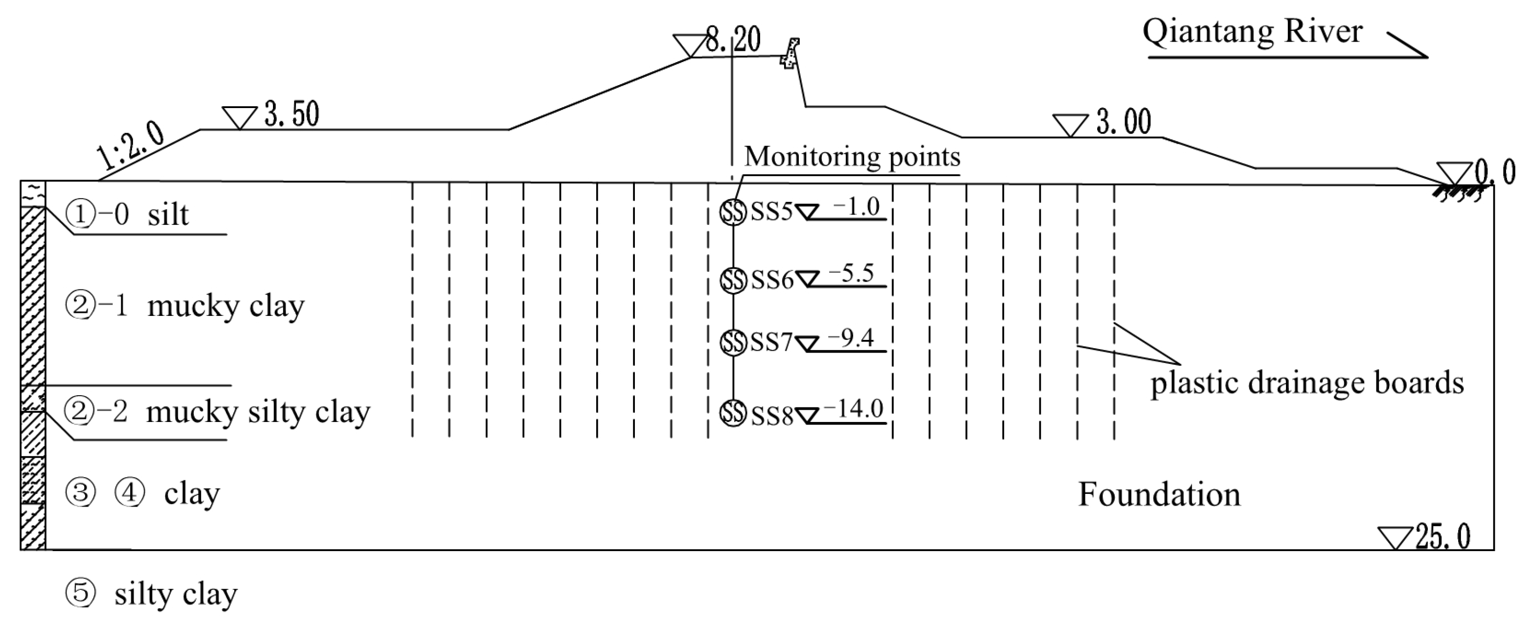
The Haiyan seawall is a vertical dike with a soil–rock mixed structure with revetments on both sides. The study area is mainly intertidal with flat terrain. The studied seawall is built on silty soft soil with an average thickness of 25.0 m, and it is reinforced by plastic drainage boards. Figure 5 exhibits the distribution of the soil layers and monitoring points. The foundation boarding is arranged in a plum blossom pattern, with a horizontal range of 36.0 m, a depth of 15.0 m, and an interval of plastic drainage boards of 1.2 m. It can be seen from the figure that the foundation includes five layers: silt layer, mucky clay layer, mucky silty clay layer, clay layer, and silty clay layer. The settlement monitoring data used in this study was collected at the maximum settlement section Z7+000, which includes four monitoring points SS5, SS6, SS7, and SS8. As the four monitoring points are selected, the prediction involves using various data points collected from multiple sources or sensors over time to predict future values. Multipoint data can capture complex interactions and dependencies between different variables, leading to more accurate and insightful predictions. These monitoring points are located at 1 m, 5.5 m, 9.4 m, and 14 m under the foundation, respectively. We used the JG86 type electromagnetic induction instrument to monitor the settlement of the seawall, which consists of a settlement measuring tube and magnetic rings. A settlement magnetic ring is placed every 3 to 4 m along the settlement measuring tube. During the construction loading period, monitoring was conducted once every 3 days.

Figure 6 shows the time variation in settlement at the selected four monitoring points at section Z7+000. Overall, the monitoring data of each of these four selected points exhibit a nonlinear upward dynamic increasing trend. Furthermore, since seawall settlement primarily stems from the consolidation of the foundation soil, the settlement curve displays rapid growth at its initial stages followed by a slower progression. As the depth of the monitoring points increases, the change in settlement gradually increases. The settlement of monitoring point SS8 ranged within 40 mm; however, the settlement of monitoring point SS5 reached up to 200 mm. This is because the soil properties change with the increase in depth, for example, the transition from looser surface soil to denser subsurface soil. This change may increase the compressibility of the deeper soil layers, resulting in greater settlement under the same external force. Additionally, the deeper soil layers are subjected to a greater weight from the overlying soil layers (i.e., vertical stress). The increased stress can cause the voids between soil particles to be compressed, thereby making the settlement more serious. Furthermore, settlement is a process that develops over time. In some cases, the settlement of deeper soil layers may gradually increase due to time-dependent effects such as soil consolidation and creep.

4. Results and Discussions

This section presents the prediction results and intermediate calculation of the proposed model. In addition, the prediction performance of the proposed model is compared to other related methods including the fractional-order GM(1,1) model, the integer-order GM(1,1) model, and fractal theory. The proposed model does not require high computer specifications. A basic configuration, such as Intel Core i5 CPU, 8 GB RAM, and 256 GB SSD, is sufficient.

4.1. Intermediate Calculation and Prediction Results

Since the modelling processes for data at each monitoring point are the same, settlement at monitoring point SS5 was selected as an example to exhibit the intermediate calculation of the proposed model. It was a data sequence containing 20 numbers, wherein 15 of them were selected as fitting data, while the remaining 5 served as testing data.

The initial order was set to 1, to make the fractional-order GM(1,1) model equivalent to the integer-order GM(1,1) model. The initial order 1 was encoded as a binary string to generate the initial population. The genetic algorithm was employed with the control parameters including a population size M of 21, crossover probability P_c of 0.75, and mutation probability P_m of 0.01, and then the evolution was carried out for 50 generations.

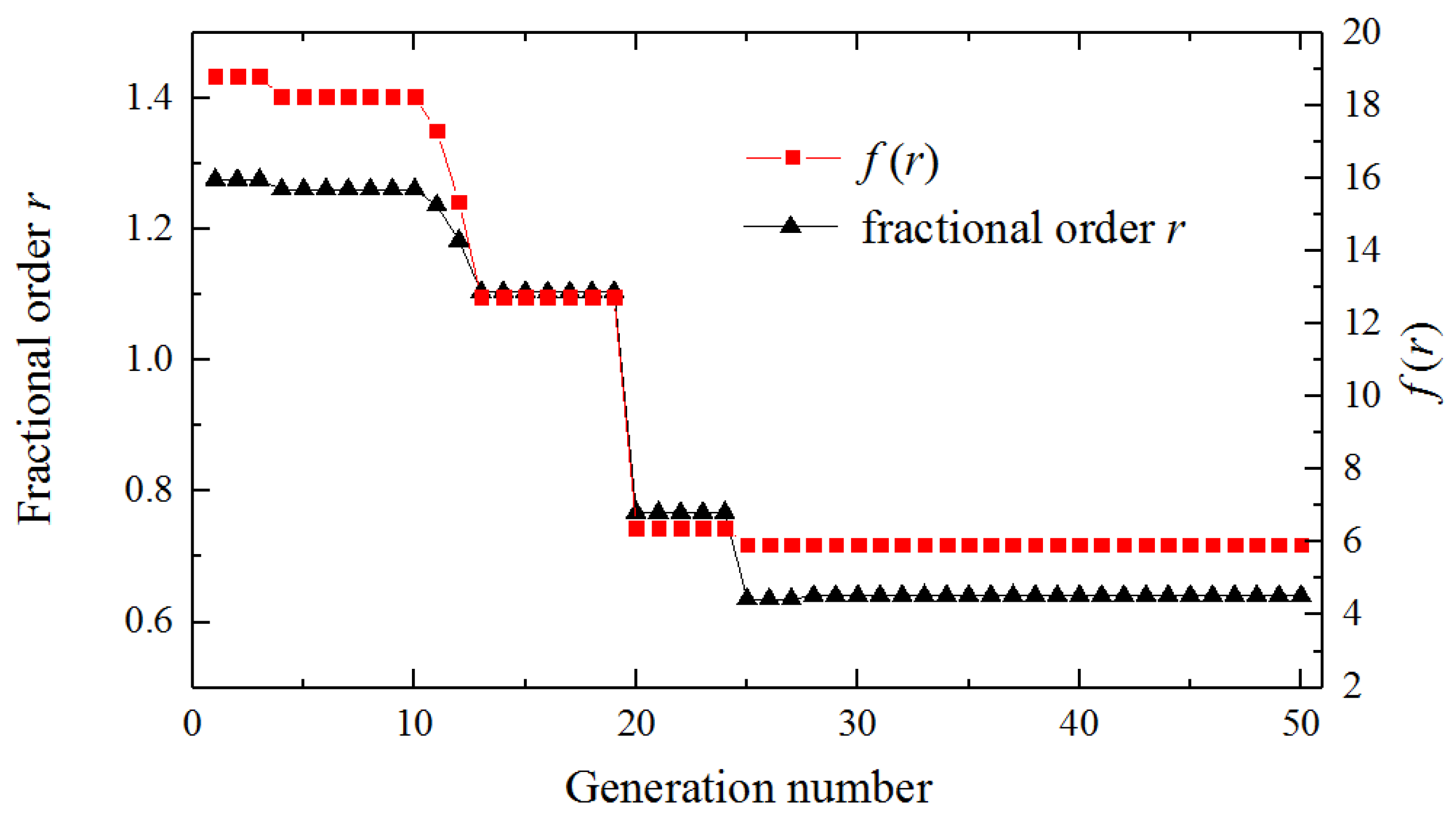
The evolution curve with respect to the genetic generations is depicted in Figure 7. The results show that the average relative error reached its minimum (i.e., 5.934) at the 38th generation, corresponding to the optimal fractional order of 0.641.

Calculated by the fractional-order grey model, the time response function can be obtained:

$${\widehat{x}}^{(0.641)}\left(k\right)=-5283.07e^{-0.012(k-1)}+5291.67.$$

The optimal fractional orders were incorporated into the fractional-order grey model using the real-time tracing algorithm, and then the settlement of the seawall can be predicted. The monitored and predicted settlement at monitoring point SS5 as well as their residual are shown in

Table 1. The monitored and predicted settlement at monitoring point SS5.

Time	Monitored Data	Predicted Data	Residual	Relative Residual
3	8.6	8.6	0	0
6	52.1	65.3	−13.24	−0.254
9	99.6	89.7	9.87	0.099
12	110.5	99.7	10.84	0.098
15	119.1	107.9	11.16	0.094
18	120.6	115.4	5.20	0.043
21	129.5	126.4	3.09	0.024
24	132.5	129.1	3.36	0.025
27	134.0	135.7	−1.73	−0.013
30	139.1	142.2	−3.13	−0.023
33	147.4	148.7	−1.32	−0.009
36	146.1	150.2	−4.12	−0.028
39	148.5	151.8	−3.26	−0.022
42	161.6	163.4	−1.78	−0.011
45	171.6	165.1	6.52	0.038
48	176.9	166.2	10.67	0.060
51	185.7	187.8	−2.12	−0.011
54	194.3	197.9	−3.59	−0.018
57	205.1	203.1	1.99	0.010
60	208.1	210.5	−2.38	−0.011

. In general, the relative residual between the monitored data and predicted data is fairly small.

Figure 8 illustrates the time evolution of the predicted and monitored settlement at each monitoring point. The red points denote the predicted data, and the black points denote the monitored data. This comparison provides valuable insights into the accuracy and reliability of the prediction model. In detail, the data sequence at each monitoring point comprises 20 data points. Among these, the first 15 data points were chosen for fitting the model, meaning they were used to calibrate the model’s parameters and ensure it accurately reflects the monitored settlement. The remaining 5 data points, set aside as testing data, served to validate the model’s predictive capabilities on unseen data. It can be seen from the figure that the monitored data aligns remarkably well with the predicted data, not only for the fitting dataset but also for the testing dataset. This strong correlation indicates that the prediction model possesses a high degree of accuracy and is capable of generalizing well to unknown data. By comparing the predicted values with the actual monitored values, we can evaluate the accuracy of our prediction model and understand the relation between different monitoring points. The monitored settlement at monitoring points SS5 and SS6 over time shows a smooth curve. The monitored settlement at monitoring points SS7 and SS8 displays different characteristics compared to SS5 and SS6, where the fluctuations during day 5 to day 20 are more obvious. The specific reasons are analyzed as follows: The primary reason for the settlement of the seawall situated on soft soil foundations is the step-by-step loading during the construction of the embankment. The loading causes the gradual expulsion of water and air from between the soil particles, reducing the voids in the soft soil. As a result, the entire foundation undergoes systematic deformation. The surface layer of the seawall foundation consists of about 50 cm of silt. Unlike the underlying soft soil, the silt has a very high water content and low structural strength. During the initial half-month period of the project, the silt would have been squeezed out to the sides along with the construction loading process, resulting in significant instantaneous settlement. Due to construction constraints, the monitoring instruments took samples with an interval of 3 days. This resulted in poor trend consistency in the collected settlement data, making it difficult for current models to accurately fit the data from day 5 to day 20.

Figure 9 illustrates the time evolution of the relative residual of the predicted and monitored settlement at each monitoring point. The relative residual is below 0.1 for all four monitoring points, which suggests that the model is capable of capturing the general trends and behaviors of the settlement process, regardless of specific local conditions. This global accuracy is crucial for providing a comprehensive understanding of the settlement phenomenon and for making informed decisions regarding potential risks and mitigation measures. In addition, the relative residual exhibits some fluctuations at the initial stage. The fluctuations in the relative residual during the initial stage likely indicates that the model is still adjusting to the initial conditions and data. This could be due to the inherent uncertainty in the initial measurements or the model’s parameters being set to approximate values. Over time, as more data is collected and the model is able to learn from these observations, the fluctuations tend to decrease, indicating the model’s ability to adapt and improve its predictions. Even though the evolution curve of the relative residual of these four monitoring points are similar globally, the fluctuations of monitoring points SS5 and SS6 are more obvious than those of monitoring points SS7 and SS8. The relative residual globally reflects the prediction accuracy. Prediction accuracy for seawall settlement can vary at different monitoring points due to several factors related to both the characteristics of the site and the limitations of the prediction model. Different monitoring points are located on varying soil types, each with unique properties such as compressibility and permeability. These properties significantly influence settlement behavior. In addition, the distribution of loads on the seawall, including static and dynamic loads from waves, tides, and human activity, may differ across monitoring points, affecting settlement rates. Thus, the historical data used for training the model vary in quality and quantity across different monitoring points, affecting the model’s ability to learn accurate patterns. For the model’s prediction ability itself, as the interactions between different influencing factors (e.g., soil properties, environmental conditions) are complex and non-linear, the present model may not capture these interactions accurately.

4.2. The Evaluation Criteria of Prediction Performance

The prediction performance of the prediction model is evaluated by calculating the coefficient of determination (R²), the mean relative error (MRE), the mean squared error (MSE), and the root mean squared error (RMSE) of the predicted results. These indexes express the extent of prediction error by measuring the deviation between the predicted data ${\alpha }_i$ and the monitored data ${\beta }_i$. The expression of MRE is shown in equation 15, and the expressions of R², MSE, and RMSE are as follows:

$$R^2=1-{\displaystyle \frac{{\displaystyle \sum _{i=1}^n\left({\alpha }_i-{\beta }_i\right)}}{{\displaystyle \sum _{i=1}^n\left({\alpha }_i-\overline{{\beta }_i}\right)}}},$$

(16)

$$MSE={\displaystyle \frac{1}{n}}{\displaystyle \sum _{i=1}^n{\left({\alpha }_i-{\beta }_i\right)}^2},$$

(17)

$$RMSE=\sqrt{{\displaystyle \frac{1}{n}}{\displaystyle \sum _{i=1}^n{\left({\alpha }_i-{\beta }_i\right)}^2}}$$

(18)

Table 2. The evaluation criteria of the proposed model at each monitoring point.

Monitoring Points	Fitting Data				Testing Data
	R2	MRE	MSE	RMSE	R2	MRE	MSE	RMSE
SS5	0.974	5.577	46.452	6.585	0.820	0.779	2.791	4.999
SS6	0.971	5.671	22.731	4.606	0.853	1.140	2.603	3.261
SS7	0.977	0.091	12.755	3.570	0.853	0.759	0.501	0.952
SS8	0.878	13.432	5.292	2.222	0.818	1.730	0.309	0.606

exhibits the evaluation criteria including the R², MRE, MSE, and RMSE of the proposed model at each monitoring point. The R², which is a measure of how much the data points are spread out from their mean, is greater than 0.8 for both the testing dataset and the fitting dataset, which implies the model is robust and can be validated. The high R² suggests that the model explains a large portion of the variation in the dependent variable, indicating a good fit. The low values of MRE, MSE, and RMSE further confirm the model’s accuracy in predicting the target variable. These evaluation criteria collectively demonstrate the model’s reliability and effectiveness.

4.3. Comparison of the Proposed Model with Other Relevant Models

To better evaluate the performance of the proposed model, we compared its prediction accuracy with the fractional-order GM(1,1), integer-order GM(1,1), and fractal theory model. The integer-order GM(1,1) is a widely used grey model which relies on the principle of differential equations and exponential smoothing to generate predictions. The fractal theory model provides a framework for modeling complex processes that exhibit self-similarity across different scales, so as to capture the inherent hierarchical patterns in the data sequence. The fractional-order GM(1,1) is a generalization of the traditional integer-order grey model, which introduces the concept of fractional-order calculus to improve the flexibility and accuracy of the model. By allowing the order of differentiation and integration to be non-integer, the fractional-order model can better capture complex and non-linear dynamics in data.

Figure 10 shows the time evolution of fitting and predicting results of seawall settlement at the selected monitoring points using these four different models. Firstly, it is noteworthy that all these four models demonstrate a certain level of accuracy in fitting the historical data and predicting future seawall settlement trends, the curve trend of the predicted value aligns precisely with the actual curve. This indicates that the predicted curve generated through each model is rational and logical, and each model has captured essential elements of the system dynamics.

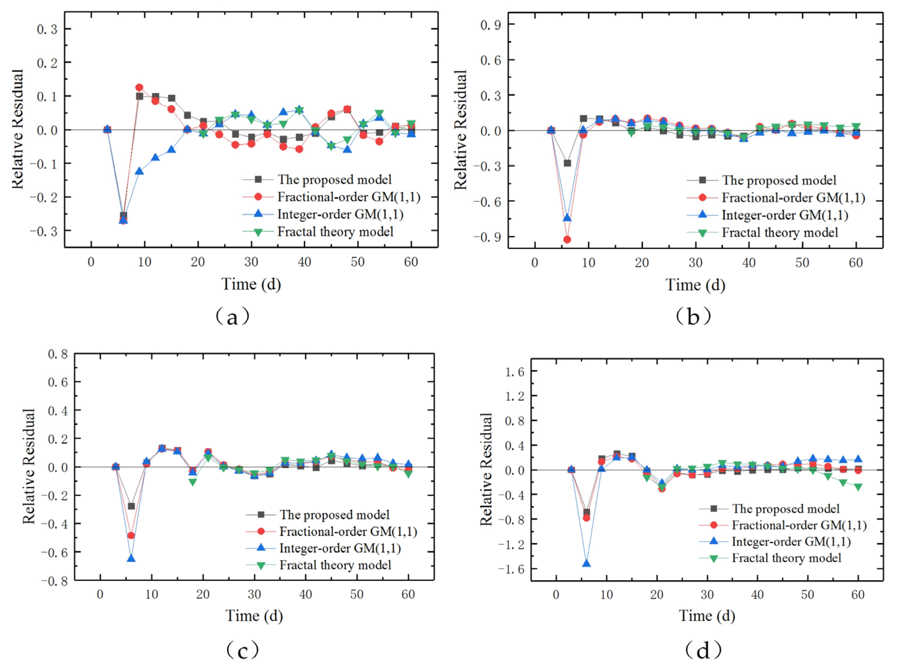
Figure 11 shows the time evolution of the relative residual of the four models for each monitoring point. The relative residuals of all four models are very small. Most are located within the range of −0.1 to 0.1. It can be seen that the proposed model shows a tighter fit to the monitoring data compared with the other three models, indicating a higher degree of accuracy. This can be evidenced by a narrower confidence interval or a high coefficient of determination between the predicted and monitored data. In addition, for all four prediction models, the relative residual exhibits some fluctuations at the initial stage. The relative residual refers to the difference between the predicted value and the actual value, normalized or scaled in a way that makes it easier to compare across different data points or time periods. These fluctuations in the relative residual at the initial stage may result from several reasons: First, the initial period does not have enough data points to accurately capture the trends, which may lead to higher errors and fluctuations in the relative residuals. Second, the models need initialization before they can start making accurate predictions. During this initial phase, the models might not be fully calibrated. Third, there might be external factors, such as measurement errors, which introduce noise and uncertainty into the predictions.

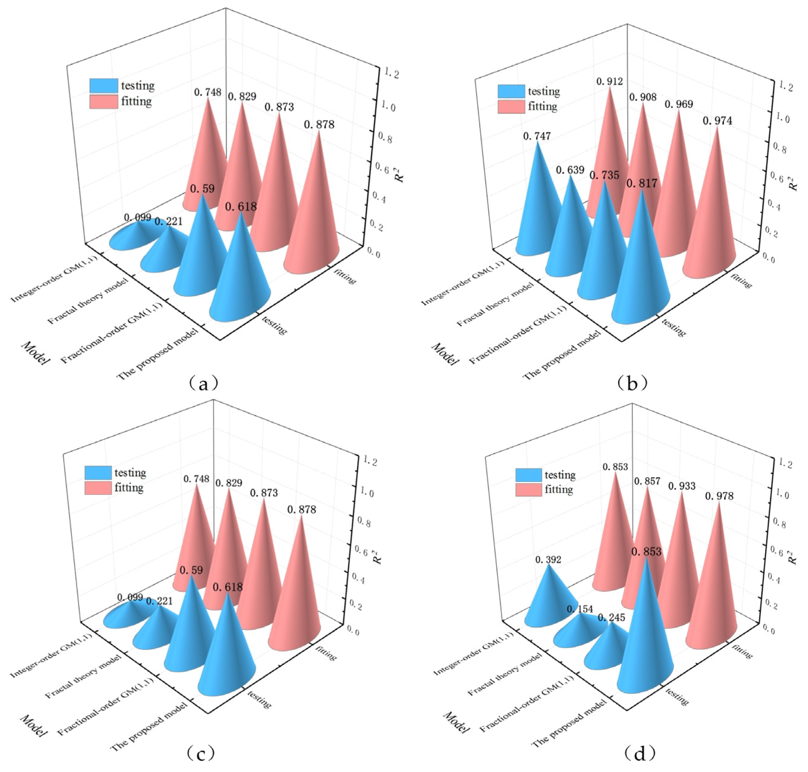
When discussing the performance of prediction models, it is important to consider not only how the models behave at different stages but also the overall accuracy. Figure 12 compares the coefficients of determination R² of the fitting and testing data for these four models, which represent an overall evaluation of the prediction performance. Using the datasets of all the monitoring points, the proposed model outperforms the other three models. The comparisons demonstrate that the proposed model exhibits superior predictive power, especially in capturing the nonlinearities and complexities of seawall settlement over time under the situation of limited data volume. Seawall settlement is affected by many factors including soil properties and hydrological conditions. A model that can accurately predict such complex processes is valuable for risk management. In addition, the R² calculated using fitting data is higher than that calculated using testing data for all these four models. It is a common observation that when the model is evaluated on testing data, which is independent of the training data, its performance tends to be lower. This is because the testing data contains additional uncertainty and variability that the model has not encountered during training.

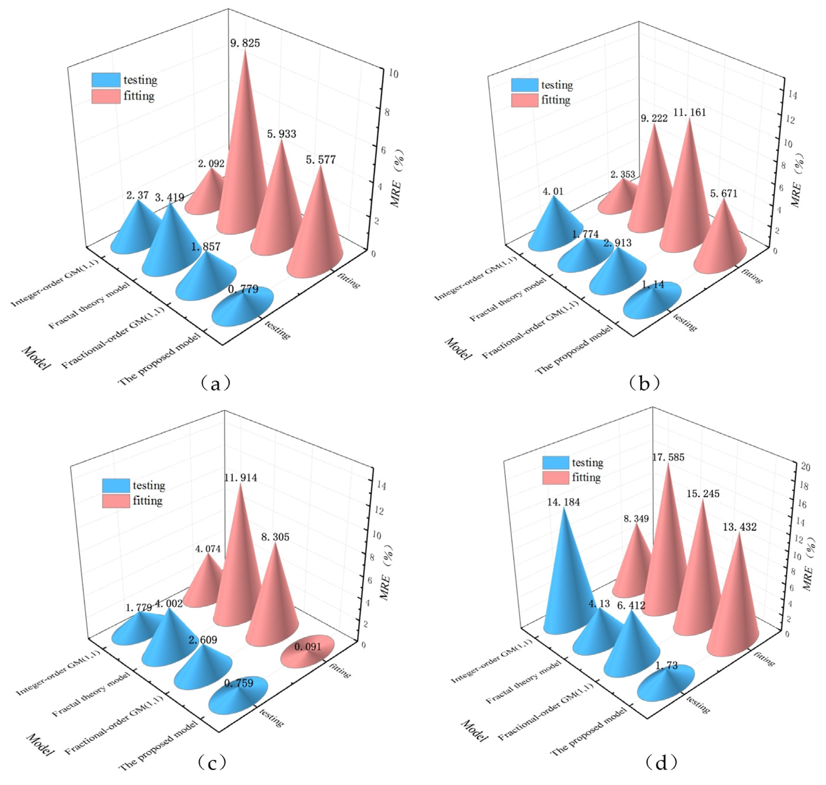
Figure 13 compares the MRE of the proposed model with the fractional-order GM(1,1), integer-order GM(1,1), and fractal theory model. A lower MRE indicates higher accuracy and better performance of the model. The proposed model exhibits a lower MRE than the other models for all monitoring points. This suggests that it is able to more accurately capture the underlying dynamics in the data sequence, leading to more reliable and accurate predictions.

5. Conclusions

As the performance of the fractional-order grey model is easily affected by the inappropriate setting of the fractional order, and considering the limited data volume and the nonlinear characteristics of seawall settlement monitoring data, this paper proposed an improved fractional-order grey model for seawall settlement prediction by integrating a genetic algorithm and the real-time tracing algorithm. First, the genetic algorithm with enhanced search capabilities was employed to solve the premature convergence problem. Then, to solve the problem of the fractional-order grey model associated with fixed step sizes, the real-time tracing algorithm was introduced to conduct equal-dimensionally recursive calculation. The proposed model was validated using monitoring data of the Haiyan seawall in Zhejiang province, China. The prediction performance of the proposed model was compared with those of the fractional-order GM(1,1), integer-order GM(1,1), and fractal theory model, demonstrating its superior performance compared to other methods such as the fractional-order GM(1,1) model, the integer-order GM(1,1) model, and fractal theory model.

The proposed model effectively predicts seawall settlement trends and can be extended to address prediction challenges in other fields with limited data volume. The significance of this finding lies in its practical implications. A reliable settlement prediction model is crucial in various engineering applications, such as construction projects, where precise forecasting of ground movements is essential for safety and stability. The high degree of fit between the predicted and monitored data suggests that the model can be trusted to provide accurate settlement predictions, thereby enhancing the safety and efficiency of related projects.

While the current model shows promising results, there are still opportunities for improvement. For example, its relatively high time complexity poses some disadvantages in terms of computation time (computational complexity of the proposed model with other models are shown in

Table 3. Computational complexity of the proposed model with other models.

Models	The Proposed Model	The fractional-Order GM(1,1)	Integer-Order GM(1,1))	Fractal Theory
Variable number of parameters	6 (including fractional-order r, population size M, crossover probability Pc, mutation probability Pm, typical number of iterations, predicted length m)	1 (fractional-order r)	0	1 (including fractal dimension D)
Calculating time	12 s	3 s	1 s	5 s

). Additionally, the model could be further refined by incorporating additional influencing factors, such as soil properties, groundwater conditions, or changes in loading conditions. Also, this paper took multi-point monitoring data into account in the prediction model, which helps to provide a comprehensive understanding of the trends of seawall settlement comparing to single-point prediction. However, one disadvantage of the current study is that the correlation among different monitoring points is not entered. Considering the correlation among each monitoring point would be interesting for further studies.