Article

An Efficient Numerical Solution of a Multi-Dimensional Two-Term Fractional Order PDE via a Hybrid Methodology: The Caputo–Lucas–Fibonacci Approach with Strang Splitting

by
Imtiaz Ahmad
1,*,
Abdulrahman Obaid Alshammari
2,
Rashid Jan
3,
Normy Norfiza Abdul Razak
3 and
Sahar Ahmed Idris
4
1
Institute of Informatics and Computing in Energy (IICE), Universiti Tenaga Nasional (UNITEN), Kajang 43000, Selangor, Malaysia
2
Department of Mathematics, College of Science, Jouf University, Sakaka 72388, Saudi Arabia
3
Institute of Energy Infrastructure (IEI), Department of Civil Engineering, College of Engineering, Universiti Tenaga Nasional (UNITEN), Putrajaya Campus, Jalan IKRAM-UNITEN, Kajang 43000, Selangor, Malaysia
4
Faculty of Engineering, Department of Industrial Engineering, King Khalid University, Abha 61421, Saudi Arabia
*
Author to whom correspondence should be addressed.
Fractal Fract. 2024, 8(6), 364; https://doi.org/10.3390/fractalfract8060364
Submission received: 29 May 2024 / Revised: 13 June 2024 / Accepted: 17 June 2024 / Published: 20 June 2024

Abstract

:
The utilization of time-fractional PDEs in diverse fields within science and technology has attracted significant interest from researchers. This paper presents a relatively new numerical approach aimed at solving two-term time-fractional PDE models in two and three dimensions. We combined the Liouville–Caputo fractional derivative scheme with the Strang splitting algorithm for the temporal component and employed a meshless technique for spatial derivatives utilizing Lucas and Fibonacci polynomials. The rising demand for meshless methods stems from their inherent mesh-free nature and suitability for higher dimensions. Moreover, this approach demonstrates the effective approximation of solutions across both regular and irregular domains. Error norms were used to assess the accuracy of the methodology across both regular and irregular domains. A comparative analysis was conducted between the exact solution and alternative numerical methods found in the contemporary literature. The findings demonstrate that our proposed approach exhibited better performance while demanding fewer computational resources.

1. Introduction

Over the last decade, there has been considerable interest in fractional partial differential equations (PDEs), making it a vibrant research field for scientists and engineers. PDEs possess the capability to describe numerous complex phenomena across diverse fields, including biology, fluid mechanics, plasma physics, optics, acoustics, financial mathematics, climate modeling, materials science, and electromagnetics [1,2]. Fractional calculus, which deals with derivatives and integrals of non-integer order, finds broad applications in science and technology. In physics, it models complex systems with non-local behavior, such as anomalous diffusion in fluid dynamics and memory effects in viscoelastic materials [3]. Engineering benefits from fractional calculus are found in signal processing, control theory, and optimization, offering robustness and efficiency in dynamic systems. Telecommunications utilize it for modeling wireless communication channels and improving channel estimation algorithms. Fractional calculus enables advancements in understanding and optimizing real-world processes and systems across various domains [4]. The fractional spatio-temporal PDE models are crucial in describing complex phenomena [5], whereas the two-scale fractal PDE models are essential for simulating intricate structures in materials science and physics, offering insights into multiscale behaviors and enhancing our understanding of fractal geometries in natural and engineered systems [6]. In particular, the Sobolev model equation is integral across various scientific fields, providing a robust framework for investigating phenomena with spatial variations. Its relevance extends across disciplines, encompassing physics, engineering, biology, and finance. In physics, Sobolev PDEs are commonly utilized to model phenomena such as heat conduction, fluid dynamics, and quantum mechanics [7,8]. Engineers employ them to analyze structural mechanics, electromagnetism, and signal-processing problems [7]. Furthermore, Sobolev PDEs find applications in image processing, medical imaging, and geophysical exploration. Their adaptability lies in their capacity to handle irregular domains and boundary conditions while providing solutions that demonstrate smoothness properties.
Numerous studies explored the applications and theoretical foundations of Sobolev PDEs, underscoring their significance in both theoretical and applied contexts. However, numerous researchers faced challenges in deriving and formulating various complex phenomena within nonlinear PDEs with integer orders [9]. In response, fractional calculus is regarded as a viable solution to this issue, as it incorporates a nonlocal property that is absent in nonlinear PDEs with integer orders [10]. Observations indicate that multi-term time-fractional PDEs were proposed to enhance the modeling accuracy in depicting anomalous diffusion processes, capturing various types of viscoelastic damping, accurately representing power-law frequency dependence, and simulating the flow of a fractional Maxwell fluid [11]. This study focused on the two-term time-fractional Sobolev equation in two and three dimensions, defined as follows:
ξ 1 U t ξ 1 + ξ 2 U t ξ 2 β t 2 U r 2 + 2 U s 2 δ 2 U r 2 + 2 U s 2 + η U 2 U r 2 + 2 U s 2 + η U r + U s 2 + γ U = F ( r , s , t ) , r , s Ω R 2 , 0 < ξ 2 ξ 1 1 , t > 0 ,
and
ξ 1 U t ξ 1 + ξ 2 U t ξ 2 β t 2 U r 2 + 2 U s 2 + 2 U z 2 δ 2 U r 2 + 2 U s 2 + 2 U z 2 + η U 2 U r 2 + 2 U s 2 + 2 U z 2 + η U r + U s + U z 2 + γ U = F ( r , s , z , t ) , r , s , z Ω R 3 , 0 < ξ 2 ξ 1 1 , t > 0 ,
with the following initial and boundary conditions:
U ( r ¯ , 0 ) = U 0 ( r ¯ ) ,
U ( r ¯ , t ) = f 1 ( r ¯ , t ) , r ¯ Ω R d , d = 2 , 3 .
where the constants β , δ , η , and γ have known values. Moreover, ξ 1 t ξ 1 and ξ 2 t ξ 2 denote the Caputo derivatives in accordance with Caputo [12] and applied to U ( r ¯ , t ) , where 0 < ξ 2 ξ 1 1 .
Several works delved into the existence and uniqueness of solutions for Sobolev equations, as documented in [13]. Ewing [14] applied the finite difference method to tackle 2D Sobolev equations. The study [15] used a computationally appealing and precise local meshless technique to provide numerical solutions for three-dimensional two- and three-term time-fractional PDE models. Various test problems were employed to assess the accuracy and reliability of the proposed approach. The paper by Luo et al. [16] introduces a reduced-order extrapolated finite difference iterative scheme for 2D Sobolev equations, employing proper orthogonal decomposition to construct a reduced-order solution space model, thus reducing the computational costs. Numerical experiments validated the scheme’s efficiency and accuracy, indicating its potential for efficient Sobolev equation solving. An accurate and efficient local meshless technique is used in the article [17] to explore numerical solutions for two-term time-fractional Sobolev models. The method approximates the solution on a uniform or scattered set of nodes, yielding sparse and well-conditioned coefficient matrices. Another paper by Luo et al. [18] introduces a novel method that employs reduced-order techniques and extrapolation within a Crank–Nicolson finite volume framework for 2D Sobolev equations. It aims to improve the computational efficiency and accuracy, showcasing promising outcomes via numerical simulations. The paper by Li et al. [19] introduces an extended mixed finite element approach for solving 2D Sobolev equations, integrating a novel formulation with stable discretization for accurate solutions and computational efficiency. Numerical experiments highlighted its effectiveness and superiority over existing methods, especially in maintaining stability and convergence properties. Heydari et al. [20] introduced a novel method that employs orthonormal Bernoulli polynomials to solve distributed-order time-fractional 2D Sobolev equations, which demonstrated accuracy through four test problems. Gao et al. [21] used the local discontinuous Galerkin finite element method to solve a particular class of 2D Sobolev equations, while another work [22] applied the weak Galerkin finite element method, providing an error estimate. Abu et al. [23] presented a method for solving time- and space-fractional Sobolev equations with Caputo fractional derivatives in n-dimensional space, utilizing the reproducing kernel Hilbert space method, which is particularly effective for Caputo class derivatives. A meshless RBFs technique for solving 2D time-fractional Sobolev equations was presented by Hussain et al. [24]. This method uses a finite difference formula for time-fractional derivative approximation and RBFs for spatial operator approximation. Using a Liouville–Caputo derivative technique for the time derivative, Ahmad et al. [25] suggested an efficient meshless method for estimating the numerical solution of 3D time-fractional Sobolev equations. Furthermore, Zhang et al. [26] used a characteristic splitting mixed finite element approach to solve convection-dominated Sobolev equations.
In response to its extensive applications, researchers explored a multitude of numerical and analytical methodologies [27,28] for addressing complex PDEs. These methods encompass various techniques, such as the alternating direction implicit method [29], the homotopy perturbation method [30], the Laplace transform technique [31], the variational approach [32,33], finite element methods (FEMs) [34], finite difference methods (FDMs) [16,35], gradient descent iterative method [36], spectral methods [37], the exp-function method [38], the alternating direction method [39], and meshless methods [40]. Notably, the straightforward nature of the FDM, FEM, and meshless techniques is noteworthy. Recently, hybrid methodologies have emerged to enhance the efficiency and accuracy of numerical solutions, including meshless methods, the method of lines utilizing Fibonacci polynomials, and combinations of the FDM and FEM.
This investigation focused on computing numerical solutions for the suggested model using a hybrid methodology based on the Caputo derivative. This approach integrates Fibonacci polynomials with the established Caputo derivative concept, exploiting the relationship between Fibonacci and Lucas polynomials. This integration provides a significant advantage in the straightforward implementation of higher-order derivatives. Moreover, the proposed approach reduces computational costs by enhancing the accuracy, even with a limited number of collocation sites. Remarkably, these polynomials find diverse real-world applications in the realm of differential equations.
Addressing boundary value problems accurately involves exploring the interplay between Chebyshev and Lucas polynomials, as demonstrated in previous studies [41,42]. For instance, the Lucas sequence was utilized to approximate integro-differential equations [43], while Lucas polynomials were applied to solve higher-order differential equations [44]. Additionally, the efficacy of a Fibonacci polynomial methodology in resolving Volterra–Fredholm integral differential equations was demonstrated [45]. Furthermore, a hybrid Taylor–Lucas polynomial approach was introduced for addressing delay difference equations [46]. Notably, novel methodologies for solving time-dependent PDEs were proposed by combining hybrid Fibonacci and Lucas polynomial schemes [47,48]. Moreover, researchers employed finite differences and Lucas polynomials to achieve effective numerical solutions for various PDE models [49,50].

Motivation

The primary objective of this research was to introduce a relatively new numerical approach designed to solve two-term time-fractional PDE models in both two and three dimensions. This method combines the Liouville–Caputo fractional derivative scheme with the Strang splitting algorithm for the temporal component and utilizes a meshless technique for spatial derivatives, incorporating Lucas and Fibonacci polynomials. Below are some of the highlighted key features of the proposed study:
  • The complex characteristics of fractional nonlinear PDEs make calculating analytical solutions challenging, driving ongoing research efforts to develop accurate and efficient numerical methodologies, with the two-term fractional order Sobolev model equation in both two and three dimensions holding significant importance across multiple scientific domains.
  • This study aimed to introduce an efficient numerical framework specifically designed for solving PDEs with temporal fractions.
  • The proposed methodology adopts a hybrid approach, integrating Fibonacci and Lucas polynomials with finite difference techniques, while also addressing the temporal direction through the utilization of the Liouville–Caputo fractional derivative in conjunction with a splitting mechanism.
  • Lucas and Fibonacci polynomials, unlike orthogonal counterparts, like Chebyshev polynomials, are non-orthogonal, eliminating the need for interval transformations. Additionally, they facilitate the straightforward approximation of higher-order derivatives for unknown functions.
  • Furthermore, the approach is characterized by its simplicity and ability to enhance the accuracy, even in scenarios involving fewer nodal points, with the aim to provide a robust and effective numerical solution to the intricate challenges posed by nonlinear PDEs.
This paper is organized as follows: Section 2 provides an overview of the fundamental terms and concepts. The proposed technique for the underlying model equations is discussed in Section 3, while theoretical results regarding stability and error analysis are presented in Section 4. Section 5 utilizes numerical experiments to validate the method’s efficacy, and finally, Section 6 summarizes the outcomes and presents concluding remarks to finalize the work.

2. Basic Concepts in Fractional Calculus and Polynomial Theory

In fractional calculus, fractional derivatives are crucial. Fractional calculus finds applications in various fields, including physics, engineering, biology, and finance, providing a powerful framework for modeling complex phenomena characterized by memory, non-locality, and fractal behavior. The fundamental definition of fractional calculus involves the generalization of differentiation and integration to non-integer orders. Here are some basic definitions of frequently used fractional derivatives.
Definition 1. 
The Riemann–Liouville derivative [51,52] is a mathematical concept used to generalize the notion of a derivative to functions that are not necessarily differentiable in the traditional sense. It is commonly applied in the field of fractional calculus to describe the behavior of functions with fractional orders of differentiation.
ξ U ( r ¯ , t ) t ξ = 1 Γ 1 ξ d d t t T ( U ( r ¯ , ϑ ) U ( r ¯ , T ) ) ( ϑ t ) ξ d ϑ , 0 < ξ < 1 .
Definition 2. 
Caputo’s fractional derivative [12] is a widely used mathematical tool in fractional calculus, providing a powerful approach for describing and analyzing non-local and memory-dependent phenomena in various scientific and engineering fields.
ξ U ( r ¯ , t ) t ξ = 1 Γ 1 ξ 0 t U ( r ¯ , ζ ) ζ t ζ ξ d ζ , 0 < ξ < 1 .
Definition 3. 
The Atangana and Baleanu fractional derivative [53], proposed by Atangana and Baleanu, is a non-local operator that extends the concept of fractional calculus. It provides a novel approach for modeling complex systems that exhibit memory and non-local behavior.
A a B C ξ U ( r ¯ , t ) t ξ = B ( ξ ) 1 ξ a t U ( r ¯ ) E ξ ξ ( t r ¯ ) ξ 1 ξ d r ¯ , 0 < ξ < 1 .
Definition 4. 
He’s fractional derivative [54]:
ξ U ( r ¯ , t ) t ξ = 1 Γ 1 ξ d d r ¯ t 0 t ( t ζ ) ξ [ U 0 ( ζ ) U ( ζ ) ] , 0 < ξ < 1 .

2.1. Fibonacci and Lucas Polynomial Theory

Below are explanations outlining the definitions, practical implications, and utilization of Lucas and Fibonacci polynomials, encompassing tasks such as approximating unfamiliar functions and their derivatives.
  • Fibonacci polynomials [49]:
The Fibonacci polynomial, which is an extension of Fibonacci numbers, is defined through a three-term recurrence relation:
F k ( r ) = k F k 1 ( r ) + F k 2 ( r ) , k 2 ,
where the sequence begins with F 0 ( r ) = 0 and F 1 ( r ) = 1 . When r = 1 , Equation (9) generates the familiar sequence of Fibonacci numbers.
  • Lucas polynomials [49]:
One can define the Lucas polynomials using the three-term recurrence relation:
L k ( r ) = k L k 1 ( r ) + L k 2 ( r ) , k 2 ,
with L 0 ( r ) = 2 and L 1 ( r ) = r as initial values. This allows Equation (10) to produce a series of Lucas numbers with r = 1 .
Lemma 1 
([49]). The kth Fibonacci polynomial F k ( r ) can be used to define the mth-order derivative of the kth Lucas polynomial L k ( r ) :
L k ( m ) ( r ) = k F k ( r ) D m 1 , D m 1 = D × D × D D ( m 1 ) time
where an ( M + 1 ) × ( M + 1 ) matrix is represented by D, which can be described as
D = 0 0 0 0 d 0 ,
where d is computed according to [49]:
d i j = i sin ( j i ) π 2 , if j > i , 0 , otherwise .

2.2. Function Approximation

Suppose U L 2 ( R ) , and let U ( r ¯ ) be continuous. Then, through the linear combination of the kth Lucas polynomials, it is possible to represent U as
U ( r ¯ ) = k = 0 Λ k L k ( r ¯ ) ,
where the Lucas polynomials are denoted as L k ( r ¯ ) , with the corresponding unknown coefficients represented by Λ k .
Likewise, U ( r ¯ ) can also be expanded under the same conditions by using a linear combination of the kth Fibonacci polynomials, as demonstrated below:
U ( r ¯ ) = k = 0 Λ k F k ( r ¯ ) .
In this context, F k ( r ¯ ) denotes the Fibonacci polynomials, while Λ k stands for the coefficients yet to be determined.
The Lucas polynomial series can be used to expand the function U ( r ¯ ) and find the first-order derivative:
U ( r ¯ ) = k = 0 Λ k L k ( r ¯ ) ,
and the function U ( r ¯ ) ’s associated m t h -order derivative is given as
U m ( r ¯ ) = k = 0 Λ k L k ( m ) ( r ¯ ) ,
where
U m ( r ¯ ) = d m U ( r ¯ ) d r ¯ m , L k ( m ) ( r ¯ ) = d m L k ( r ¯ ) d r ¯ m .
Equations (13) and (14) can be written by incorporating the relation (11):
U ( r ¯ ) = k = 0 Λ k k F k ( r ¯ ) ,
and similarly, the mth derivative can be computed as
U ( m ) ( r ¯ ) = k = 0 Λ k k F k ( r ¯ ) D m 1 ,
in which D and D m 1 are defined above.
Remark 1. 
In numerical computations, the expansion of U ( r ¯ ) and its mth derivative often involves utilizing truncated Fibonacci and Lucas polynomial series. In other words, we take
U ( r ¯ ) k = 0 M Λ k L k ( r ¯ ) , M N ,
and
U ( m ) ( r ¯ ) k = 0 M Λ k L k ( m ) ( r ¯ ) = k = 0 M Λ k k F k ( r ¯ ) D m 1 , M N ,

3. Suggested Methodology

This section is devoted to formulating the suggested meshless method for approximating the 2D time-fractional Sobolev model equations given in Equations (20) and (21). To simplify the notation throughout the discussion in this section, we introduce the following:
U n + 1 ( r ¯ ) = U ( r , s , t n + 1 ) , U i j n + 1 = U ( r i , s j , t n + 1 ) ,
where r i and s j are the collocation points specified as follows, and t n = n × δ t , with δ t representing the time step size:
r i = a + i h r , s j = c + j h s , ( i , j   =   1 ,   2 ,   ,   M , M N ) ,
where h r = ( b a ) / M and h s = ( d c ) / M are the mesh step sizes in the r and s spatial directions throughout the spatial domain Ξ = [ a , b ] × [ c , d ] R 2 .

3.1. Time Discretization

The widely recognized L 1 -formula, with 𝒪 ( δ t 2 ξ 1 ) as the approximation order error, where 0 < ξ 1 1 , is utilized to derive the discrete representation of the ( n + 1 ) th time level, as outlined in [55,56].
ξ 1 U ( r ¯ , t n + 1 ) t ξ 1 = 1 Γ ( 1 ξ 1 ) 0 t n + 1 U ( r ¯ , ζ ) ζ ( t n + 1 ζ ) ξ 1 d ζ , = 1 Γ ( 1 ξ 1 ) j = 0 n j × δ t ( j + 1 ) × δ t U ( r ¯ , ζ ) ζ ( t n + 1 ζ ) ξ 1 d ζ , = 1 Γ ( 1 ξ 1 ) j = 0 n U j + 1 ( r ¯ ) U j ( r ¯ ) δ t + O ( δ t ) j × δ t ( j + 1 ) × δ t ( ( j + 1 ) δ t ζ ) ξ 1 d ζ .
Following integration, it gives
ξ 1 U ( s , r , t n + 1 ) t ξ 1 = A ξ 1 j = 0 n K ξ 1 ( j ) U n j + 1 ( r ¯ ) U n j ( r ¯ ) + O ( δ t 2 ξ 1 ) , 0 < ξ 1 < 1 , U n + 1 ( r ¯ ) U n ( r ¯ ) δ t + O ( δ t ) , ξ 1 = 1 ,
where A ξ 1 = δ t ξ 1 Γ ( 2 ξ 1 ) and K ξ 1 ( j ) = ( j + 1 ) 1 ξ 1 ( j ) 1 ξ 1 . Therefore, we may write the following for 0 < ξ 1 < 1 after ignoring the error term:
ξ 1 U ( r ¯ , t n + 1 ) t ξ 1 = A ξ 1 U n + 1 ( r ¯ ) U n ( r ¯ ) + A ξ 1 j = 1 n K ξ 1 ( j ) U n j + 1 ( r ¯ ) U n j ( r ¯ ) ,
with K ξ 1 ( j ) = 1 and j = 0 . The fractional derivative of order ξ 2 can be found above.
Before applying the θ -weighted rule to the suggested Equations (1)–(4), let us rewrite them in compact form as follows:
ξ 1 U ( r ¯ , t ) t ξ 1 + ξ 2 U ( r ¯ , t ) t ξ 2 β 2 U ( r ¯ , t ) t δ 2 U ( r ¯ , t ) η U ( r ¯ , t ) U ( r ¯ , t ) + γ U ( r ¯ , t ) = f ( r ¯ , t ) , r ¯ Ω R d , d = 2 , 3 , 0 < ξ 2 ξ 1 1 , t > 0 ,
with the following conditions:
U ( r ¯ , 0 ) = U 0 ( r ¯ ) , U ( r ¯ , t ) = f 1 ( r ¯ , t ) , r ¯ Ω ,
where the Laplacian and gradient operators are represented by the symbols 2 and ∇, respectively.
The θ -weighted rule is now applied, and Equation (20) becomes
A ξ 1 U n + 1 ( r ¯ ) + A ξ 2 U n + 1 ( r ¯ ) β 2 U n + 1 ( r ¯ ) 2 U n ( r ¯ ) δ t θ δ 2 U n + 1 ( r ¯ ) + θ γ U n + 1 ( r ¯ ) θ U n + 1 ( r ¯ ) U n + 1 ( r ¯ ) = A ξ 1 U n ( r ¯ ) + A ξ 2 U n ( r ¯ ) + ( 1 θ ) δ 2 U n ( r ¯ ) + ( 1 θ ) η U n ( r ¯ ) U n ( r ¯ ) ( 1 θ ) γ U n ( r ¯ ) + f θ n + 1 ( r ¯ ) Q ξ n ( r ¯ ) ,
where
f θ n + 1 ( r ¯ ) = θ f n + 1 ( r ¯ ) + ( 1 θ ) f n ( r ¯ ) ,
and
Q ξ n ( r ¯ ) = A ξ 1 j = 1 n K ξ 1 ( j ) U n j + 1 ( r , s ) U n j ( r , s ) + A ξ 2 j = 1 n K ξ 2 ( j ) U n j + 1 ( r , s ) U n j ( r , s ) .
Since
U n + 1 ( r ¯ ) U n + 1 ( r ¯ ) = U n + 1 ( r ¯ ) 2 U n + 1 ( r ¯ ) + U x n + 1 ( r ¯ ) 2 + U y n + 1 ( r ¯ ) 2 ,
the nonlinear terms are linearized as follows [24]:
U n + 1 ( r ¯ ) 2 U n + 1 ( r ¯ ) U n + 1 ( r ¯ ) 2 U n ( r ¯ ) + U n ( r ¯ ) 2 U n + 1 ( r ¯ ) 2 U n ( r ¯ ) 2 U n ( r ¯ ) ,
U r n + 1 ( r ¯ ) 2 2 U r n ( r ¯ ) U r n + 1 ( r ¯ ) U r n ( r ¯ ) 2 ,
U s n + 1 ( r ¯ ) 2 2 U s n ( r ¯ ) U s n + 1 ( r ¯ ) U s n ( r ¯ ) 2 .
The insertion of Equations (23)–(25) and simple rearrangement reduces Equation (22) to
A ξ 1 + A ξ 2 + θ γ θ 2 U n ( r ¯ ) U n + 1 ( r ¯ ) β δ t + θ δ θ η U n ( r ¯ ) 2 U n + 1 ( r ¯ )
= A ξ 1 + A ξ 2 ( 1 θ ) γ U n ( r ¯ ) β δ t ( 1 θ ) δ 2 U n ( r ¯ ) + H θ n + 1 ( r ¯ ) G θ n ( r ¯ ) ,
where
H θ n + 1 ( r ¯ ) = f θ n + 1 Q ξ n U n ( r ¯ ) , n 1 , f θ 1 , n = 1 ,
and
G θ n ( r ¯ ) = η θ 2 U n ( r ¯ ) 2 U n ( r ¯ ) + U x n ( r ¯ ) 2 + U y n ( r ¯ ) 2 + ( 1 θ ) η U n ( r ¯ ) U n ( r ¯ ) .
Let us label
p θ n ( r ¯ ) = A ξ 1 + A ξ 2 + θ γ θ η 2 U n ( r ¯ ) , q θ n = β δ t + δ θ θ η U n ( r ¯ ) , r θ = A ξ 1 + A ξ 2 ( 1 θ ) γ , s θ = β δ t ( 1 θ ) δ ,
which, when substituted into Equation (26), give us
p θ n U n + 1 ( r ¯ ) q θ n 2 U n + 1 ( r ¯ ) = r θ U n ( r ¯ ) + s θ 2 U n ( r ¯ ) + H θ n + 1 ( r ¯ ) G θ n ( r ¯ ) .
We have approximated in the time direction at this point using Equation (29). Furthermore, the time direction is coupled with the splitting technique known as the Strang splitting algorithm, which is given as follows [4,57,58,59]:
U 1 t = L 1 U 1 ( t ) with t [ t n , t n + 1 / 2 ] and U 1 ( t n ) = U s p n
U 2 t = L 2 U 2 ( t ) with t [ t n , t n + 1 ] and U 2 ( t n ) = U 1 ( t n + 1 / 2 )
U 3 t = L 1 U 3 ( t ) with t [ t n + 1 / 2 , t n + 1 ] and U 3 ( t n + 1 / 2 ) = U 2 ( t n + 1 )
where L 1 U ( t ) = δ 2 U ( t ) η U 2 U ( t ) , L 2 U ( t ) = η U ( t ) 2 γ U ( t ) , and U s p n = U 0 is the initial solution defined for Equation (20). The Strang splitting method achieves second-order accuracy. Further information can be found in reference [4].

3.2. Spatial Discretization

We can expand the function U ( r ¯ ) , which is a two-dimensional function denoted as U ( r , s ) , into the following truncated series of Lucas polynomials, expressed as a product:
U ( r , s ) k = 0 M m = 0 M Λ k m L k ( r ) L m ( s ) = k = 0 M m = 0 M Λ k m L k m ( r , s ) ,
where L k m ( r , s ) = L k ( r ) L m ( s ) . Equation (33) can be expressed in compact form as
U ( r , s ) L T ( r , s ) Λ ,
with Λ = [ Λ 00 , Λ 01 , Λ 10 , , Λ M M ] T and L T ( r , s ) = [ L 00 ( r , s ) , L 01 ( r , s ) , L 10 ( r , s ) , , L M M ( r , s ) ] .
One can compute and briefly represent the consolidated partial derivatives of U ( r , s ) as follows:
U ( r , s ) r k = 0 M m = 0 M Λ k m d L k ( r ) d r L m ( s ) = k = 0 M m = 0 M Λ k m k ( F k ( r ) ) L m ( s ) = L r T ( r , s ) Λ ,
and
2 U ( r , s ) r 2 k = 0 M m = 0 M Λ k m d 2 L k ( r ) d r 2 L m ( s ) = k = 0 M m = 0 M Λ k m k ( F k ( r ) D ) L m ( s ) = L r r T ( r , s ) Λ ,
where
L r T ( r , s ) = { r L k m ( r , s ) } k , m = 0 M = { d L k ( r ) d r L m ( s ) } k , m = 0 M = { k ( F k ( r ) ) L m ( s ) } k , m = 0 M ,
L r r T ( r , s ) = { 2 r 2 L k m ( r , s ) } k , m = 0 M = { d 2 L k ( r ) d r 2 L m ( s ) } k , m = 0 M = { k ( F k ( r ) D ) L m ( s ) } k , m = 0 M .
Similarly
U ( r , s ) s k = 0 M m = 0 M Λ k m L k ( r ) d L m ( s ) d r = k = 0 M m = 0 M Λ k m m L k ( r ) ( F m ( s ) ) = L s T ( r , s ) Λ ,
and
2 U ( r , s ) s 2 k = 0 M m = 0 M Λ k m L k ( r ) d 2 L m ( s ) d s 2 = k = 0 M m = 0 M Λ k m m L k ( r ) ( F m ( s ) D ) = L s s T ( r , s ) Λ ,
with
L s T ( r , s ) = { s L k m ( r , s ) } k , m = 0 M = { L k ( r ) d 2 L m ( s ) d s 2 } k , m = 0 M = { m L k ( r ) ( F m ( s ) ) } k , m = 0 M .
L s s T ( r , s ) = { 2 s 2 L k m ( r , s ) } k , m = 0 M = { L k ( r ) d 2 L m ( s ) d s 2 } k , m = 0 M = { m L k ( r ) ( F m ( s ) D ) } k , m = 0 M .
These results can be further refined as
U ( r , s ) = U r + U s L r T ( r , s ) + L s T ( r , s ) Λ .
2 U ( r , s ) = 2 U r 2 + 2 U s 2 L r r T ( r , s ) + L s s T ( r , s ) Λ .
It is consequently possible to express the time-dependent function U ( r , s , t ) and its compact form partial derivatives as follows:
U ( r , s , t ) L T ( r , s ) Λ ( t ) , 2 U ( r , s , t ) r 2 L r r T ( r , s ) Λ ( t ) , 2 U ( r , s , t ) s 2 L s s T ( r , s ) Λ ( t ) ,
with
U ( r , s , t ) L r T ( r , s ) + L s T ( r , s ) Λ ( t ) , 2 U ( r , s , t ) L r r T ( r , s ) + L s s T ( r , s ) Λ ( t ) ,
where Λ ( t ) represents the vector of the time-varying unknown coefficients. Once the information obtained from Equations (37) and (38) is combined with Equation (29), we obtain
p θ n L ( r , s ) Λ n + 1 q θ n L r r T ( r , s ) + L s s T ( r , s ) Λ n + 1 = r θ L ( r , s ) Λ n + r θ L r r T ( r , s ) + L s s T ( r , s ) Λ n + H θ n + 1 ( r , s ) G θ n ( r , s ) , ( r , s ) Ω .
The boundary conditions are stated as
B L ( r , s ) Λ n + 1 f 1 ( r , s , t n + 1 ) = f 1 n + 1 ( r , s ) , ( r , s ) Ω ,
where Λ n = Λ ( t n ) .

3.3. Full Discretization

We collocate Equations (39) and (40) at discrete mesh points r i and s j at their respective time levels to derive the discrete form of the time-fractional differential equation as expressed in Equation (20), resulting in the subsequent set of equations:
p θ n L ( r i , s j ) Λ n + 1 q θ n L r r T ( r i , s j ) + L s s T ( r i , s j ) Λ n + 1 = s θ L ( r i , s j ) Λ n + r θ L r r T ( r i , s j ) + L s s T ( r i , s j ) Λ n + H θ n + 1 ( r i , s j ) G θ n ( r i , s j ) , ( r i , s j ) Ω ,
and
B L ( r i , s j ) Λ n + 1 f 1 ( r i , s j , t n + 1 ) = f 1 n + 1 ( r i , s j ) , ( r i , s j ) Ω ,
where i , j = 0 , 1 , 2 , , M . This implies the following matrix–vector form:
G Λ n + 1 = H Λ n + Q n + 1 .
In this case, the matrix entries are provided by
( G ) i j = p θ n L ( r i , s j ) q θ n L r r T ( r i , s j ) + L s s T ( r i , s j ) , ( r i , s j ) Ω , B L ( r i , s j ) , ( r i , s j ) Ω ,
( H ) i j = s θ L ( r i , s j ) + r θ L r r T ( r i , s j ) + L s s T ( r i , s j ) , ( r i , s j ) Ω , 0 , ( r i , s j ) Ω ,
and
( Q ) i j = H θ n + 1 ( r i , s j ) G θ n ( r i , s j ) , ( r i , s j ) Ω , f 1 ( r i , s j , t n + 1 ) , ( r i , s j ) Ω .
The construction of the scheme for the two-dimensional model equation is finalized. Simplifying it to a one-dimensional form involves eliminating the variable s so that r ¯ = r . The linear system represented by Equation (41) benefits from the assurances provided by [47], ensuring the existence of a solution. Solving Equation (41) allows for the determination of the vector containing unknown coefficients at every time step. The initial condition allows for initialization in the following manner:
L T ( r i , s j ) Λ 0 = U ( r i , s j , 0 ) = U 0 A Λ 0 = U 0 .
When solved, it yields Λ 0 . Utilizing Equation (41), the iteration is subsequently repeated up to the relevant time level. Upon obtaining the coefficients vector, the solution at the corresponding time level can be determined by
U ( r i , s j , t n ) = L T ( r i , s j ) Λ n , ( r i , s j ) Ω , ( n 0 ) .
A similar procedure can be used in the case of a three-dimensional problem.

4. Analyzing Errors

To conduct the error analysis, we referred to the following theorem.
Theorem 1. 
The error can be defined as follows when denoting the exact solution as U ^ and the computed solution obtained by the suggested meshless method as U for the underlying problems.
The error term E is constrained within the following expression:
| E | 4 exp ( 2 κ ) cosh 2 ( 2 P ) κ 2 ( N + 1 ) ( ( N + 1 ) ! ) 2 .
Proof. 
Consider the absolute error between the exact solution and the approximate numerical solution using the proposed hybrid meshless method:
| E | = | U ^ U | ,
where U ^ = k = 0 m = 0 Λ k Λ m L k ( r ) L m ( s ) and U = k = 0 M m = 0 M Λ k Λ m L k ( r ) L m ( s ) . Next, the truncated term is as follows:
| E | = k = N + 1 m = N + 1 Λ k Λ m L k ( r ) L m ( s )
In [60], it is demonstrated that
L m ( r ) 2 ϑ m ,
| Λ m | P m cosh ( 2 P ) m ! ,
where the famous golden ratio is denoted by ϑ . Consequently, Equation (45) suggests that
| E | = 4 cosh 2 ( 2 P ) k = N + 1 m = N + 1 κ k + m k ! m ! ,
where κ = P ϑ . This inequality can alternatively be expressed as
| E | = 4 exp ( 2 κ ) cosh 2 ( 2 P ) 1 Γ ( N + 1 , κ ) Γ ( N + 1 ) 2 .
The incomplete gamma function in this case is Γ ( N + 1 , κ ) , and the complete gamma function is Γ ( N + 1 ) [61]. Equation (46) can be expressed in integral form as follows:
| E | 4 exp ( 2 κ ) cosh 2 ( 2 P ) ( N ! ) 2 0 κ t N exp ( t ) d t 2 .
Since exp ( t ) < 1 , t > 0 , we obtain:
| E | 4 exp ( 2 κ ) cosh 2 ( 2 P ) κ 2 ( N + 1 ) ( ( N + 1 ) ! ) 2 .

Stability Analysis

The stability of the meshless method is crucial for ensuring the accuracy and convergence of numerical solutions over time. By mitigating numerical instabilities, the meshless method maintains the solution quality and reliability across diverse computational domains. The stability analysis was carried out in this work by utilizing a matrix technique. The methodology employed was consistent with that described in previous studies [24,62].
Theorem 2. 
Consider w as the computed approximate solution to the underlying problem. In this context, the amplification matrix ϝ is defined as F = L G 1 H L 1 . It is essential to confirm that the absolute maximum eigenvalue of ϝ, denoted as ρ ( F ) , stays less than or equal to 1 to ensure stability.
Proof. 
We aim to show that F = L G 1 H L 1 . From Equation (17), we write
Λ n = L 1 U n .
The relationship can be described utilizing Equation (41):
U n + 1 = L G 1 H L 1 U n + L G 1 Q n + 1 .
Moreover, the error vector
E = U ^ U ,
satisfies the following condition:
E n + 1 = F E n .
Thus, the amplification matrix is defined as F = L G 1 H L 1 . Adherence to the Lax–Richtmyer stability criterion [63], which requires that
| | F | | 1 ,
ensures the stability of the method. An illustration demonstrating that the spectral radius ρ ( F ) must not exceed 1 to fulfill this condition is provided in the subsequent section. □

5. Discussion and Numerical Results

The proposed hybrid meshless method (HMM) was assessed for its effectiveness and precision in solving model Equations (1) and (2). The evaluation includes various scenarios with both uniform and scattered nodes in non-rectangular and rectangular domains. The CPU time was measured in seconds for all cases. All computations were performed on an HP PC laptop equipped with an Intel(R) Core(TM) i5-7200U CPU @ 2.50 GHz 2.71 GHz and 8 GB of RAM, using MATLAB (R2012a) software.
The accuracy was measured using error norms, including the following:
e = max ( | U ^ U | ) , e r m s = i = 1 N U ^ i U i 2 N , e L 2 = δ h h = 1 N U ^ h U h 2 ,
where the exact solution is U ^ , while the approximate solution is U .
Problem 1. 
The exact solution of model (1) with δ = 1 and η = γ = 0 is
U ( r ¯ , t ) = e t sin ( π r ) sin ( π s ) , r ¯ = ( r , s ) Ω .
The numerical results of the proposed hybrid meshless method were used to compute the numerical solution of Problem 1, as shown in Table 1. The e norm was obtained for the final times t = 1 and t = 5 . The obtained numerical results were compared with the method reported in [17]. The results using explicit, implicit, and Crank–Nicolson schemes for the proposed method were computed for different time step sizes, and one could conclude that as the time step size δ t decreased, the accuracy of the proposed method increased. The comparison shows that the HMM was more accurate than the method given in [17]. In Table 2, the numerical results are presented, where they were computed by the proposed method using different fractional orders ξ, various nodal points N, δ t = 0.001 , and t = 1 . The results were computed as e and e r m s norms. It can be observed that increasing the number of nodes improved the accuracy to some extent, whereas changing the fractional order did not significantly affect the accuracy. In this case, the HMM yielded good and accurate results. Additionally, the CPU time is provided in this table, demonstrating the efficiency of the suggested method.
Comparative results of the HMM and [17] are presented in Figure 1 for various nodes in the form of different error norms. It can be observed that the results produced by the HMM were superior to those of [17]. Furthermore, Figure 2 depicts the comparison of the numerically computed solution with the exact solution, along with the absolute error.
Problem 2. 
Consider the model Equation (1) with β = 1 and γ = δ = 0 having the exact solution
U ( r ¯ , t ) = e r s t sin ( π r ) sin ( π s ) , r ¯ = ( r , s ) Ω .
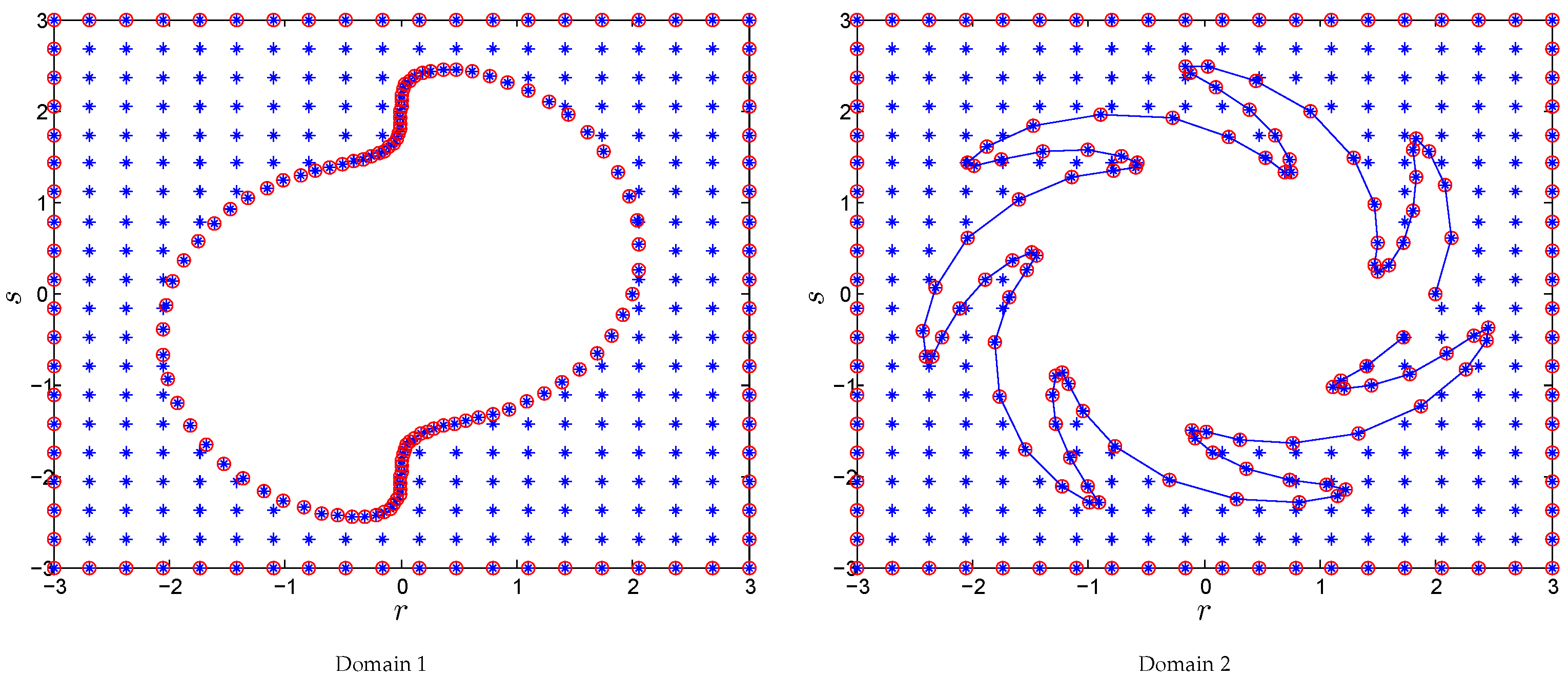
Meshless methods offer the advantage of computing solutions without being constrained by the computational geometry. These methods naturally adjust to the geometry of the domain and offer greater flexibility in handling boundary conditions. Additionally, meshless methods often exhibit excellent scalability and parallelizability, making them suitable for large-scale simulations. To assess the true effectiveness of the proposed meshless method, various irregular geometries were examined. To evaluate the performance of the proposed HMM in non-rectangular domains, as shown in Figure 3 for Problem 2, Table 3 presents the numerical results obtained using ξ 1 = ξ 2 = 0.5 and δ t = 0.0001 , along with various time values, in comparison with the method outlined in [17]. The table illustrates that the HMM achieved greater accuracy compared with [17]. Additionally, in Table 4, the numerical outcomes derived from the proposed HMM were utilized to compute the e L 2 norm for δ t , which was then compared with the results obtained using the method reported in [17]. Employing explicit, implicit, and Crank–Nicolson schemes, the proposed method’s results were calculated for different time step sizes, demonstrating that decreasing δ t enhanced the accuracy of the proposed approach. This comparison highlights the superior performance of the HMM over the method described in [17].
Figure 4 presents a comparison of the HMM results with those in [17] using various error norms for different fractional orders ξ. Once again, the HMM demonstrated superior performance. Figure 5 illustrates the close agreement between the exact and numerical solutions of Problem 2 with the parameters ξ = 0.5 , N = 10 2 , δ t = 0.001 , and time t = 0.5 in terms of the absolute error.
Problem 3. 
The exact solution of model (2) with δ = 1 and η = γ = 0 is as follows:
U ( r ¯ , t ) = e t sin ( π r ) sin ( π s ) sin ( π z ) , r ¯ = ( r , s , z ) Ω .
The results for Problem 3 were compared with the exact solution and the approach provided in [15] for different values of δ t , N = 10 , and using t = 1 and ξ 1 = ξ 2 = 0.3 . This served to illustrate the accurateness and effectiveness of the suggested strategy. These findings are presented in Table 5, along with the CPU time. The table shows that after a few iterations, the suggested meshless technique yielded better results. The accuracy also improved with an increase in the number of iterations, with both error norms reaching as low as 10 10 .
The findings of Problem 3 were computed using the proposed HMM in Table 6, with varying values of fractional order ξ for N = 10 , t = 1 , and t = 2 . We evaluated the outcomes in terms of e r m s and e . Accurate results were found for several time-fractional orders in this problem, and these results were also compared with the findings published in [15].
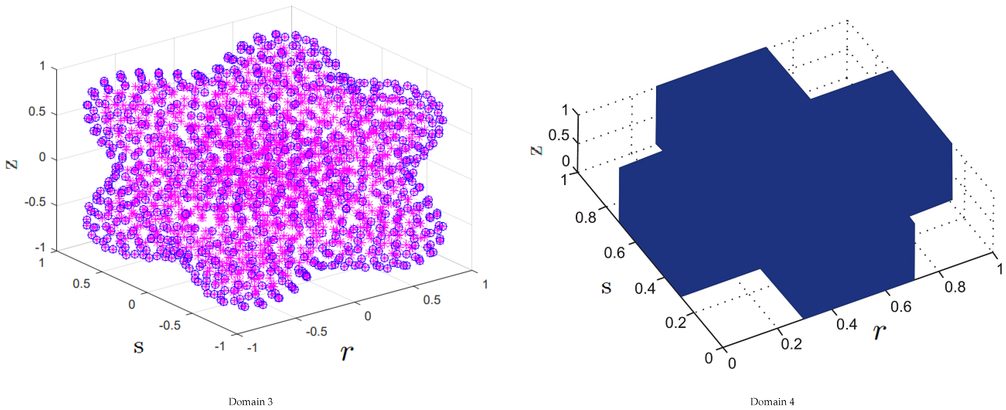
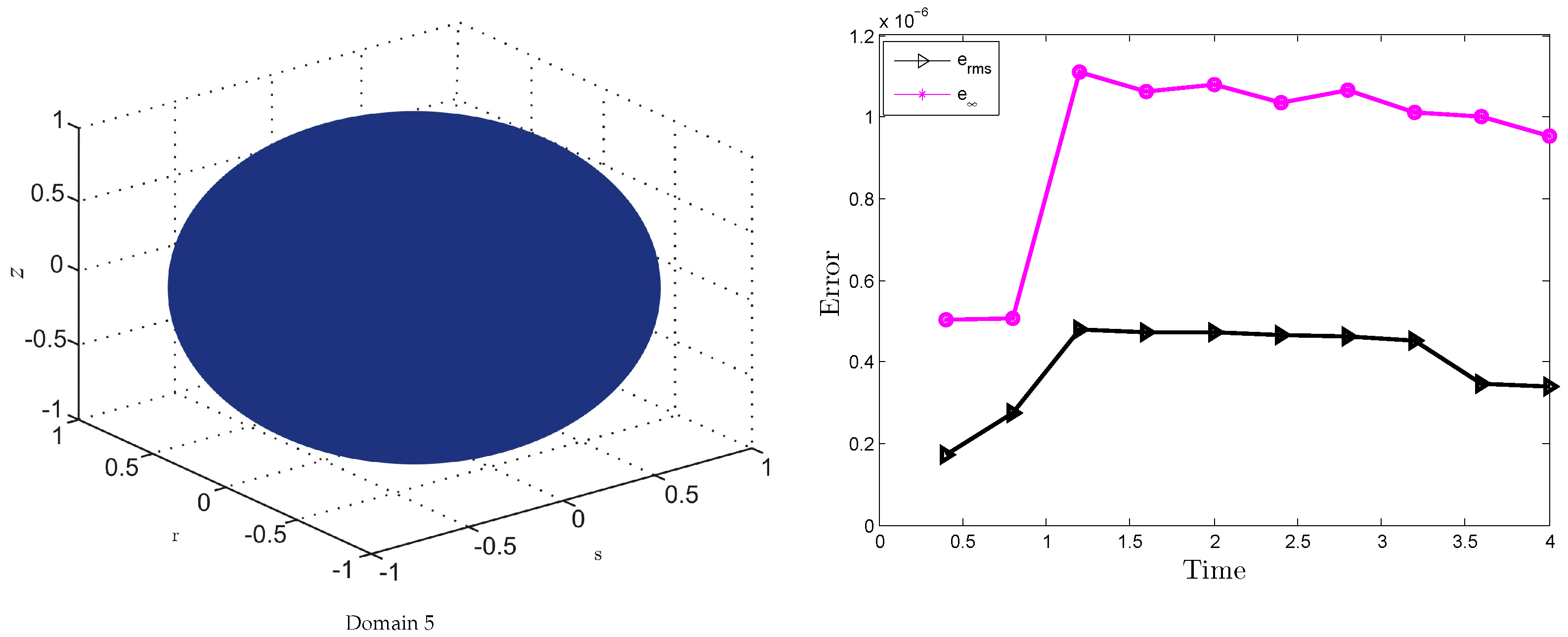
For Problem 3, we considered some non-rectangular domains shown in Figure 6 and in Figure 7 (left) to evaluate the performance of the suggested HMM. In domain 3, scattered nodes were taken into account, as shown in Figure 6 (left). The results obtained in this case are shown in Figure 8, whereas the results for domain 5 are shown in Figure 7 (right) for final times up to t = 4 . These results provide evidence of the accurate performance of the HMM in non-rectangular domains.
Problem 4. 
The exact solution for Equation (2) with β = 1 , γ = 1 , and δ = π 2 is
U ( r ¯ , t ) = e t sin ( π r ) sin ( π s ) sin ( π z ) , r ¯ = ( r , s , z ) Ω .
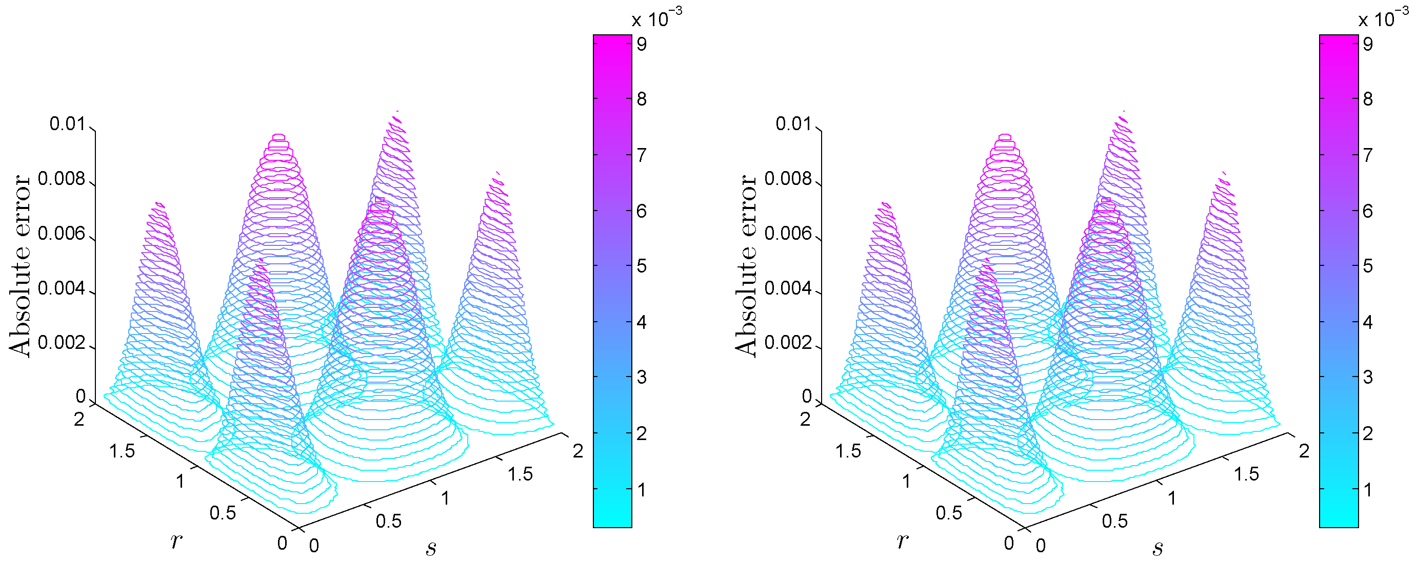
For Problem 4, the behavior of the numerical and exact solutions using N = 21 and t = 0.01 are visualized in Figure 9 at z = 0.5 and ξ 1 = ξ 2 = 0.5 , along with the absolute error. One can see from these figures that the approximate solution was very compatible with the exact solution. Also, Figure 10 shows the contour graph of the problem at ξ 1 = ξ 2 = 0.3 and ξ 1 = ξ 2 = 0.9 .

6. Conclusions

This paper introduces a relatively new numerical methodology for addressing two-term time-fractional PDE models in two and three dimensions. We combined the Louiville–Caputo fractional derivative scheme with the Strang splitting algorithm for the temporal component and employed a meshless technique for spatial derivatives utilizing Lucas and Fibonacci polynomials. Error norms were utilized to evaluate the accuracy of the methodology across regular and irregular domains. A comparative study was conducted between the exact solution and alternative numerical methods outlined in the contemporary literature. This inquiry illustrated that the proposed approach yielded superior performance while requiring reduced computational resources. Moreover, the study illustrated how minimizing the errors could be accomplished by refining the spatial and temporal stages. With minor modifications, the proposed approach could be applied to various intricate fractional partial differential equations that arise in fields such as fluid dynamics, quantum mechanics, and financial mathematics, where they model phenomena with significant spatial and temporal dependencies.

Author Contributions

Conceptualization, I.A.; Methodology, I.A. and A.O.A.; Software, A.O.A.; Validation, R.J.; Formal analysis, N.N.A.R.; Investigation, I.A. and R.J.; Resources, R.J., N.N.A.R. and S.A.I.; Data curation, N.N.A.R. and S.A.I.; Writing—original draft, I.A. and R.J.; Writing—review & editing, A.O.A., N.N.A.R. and S.A.I.; Visualization, R.J.; Supervision, N.N.A.R. and S.A.I.; Project administration, N.N.A.R.; Funding acquisition, I.A. and S.A.I. All authors read and agreed to the published version of this manuscript.

Funding

The authors extend their appreciation to the Deanship of Scientific Research at King Khalid University for funding this work through Large Groups (project under grant number 2/478/44).

Data Availability Statement

Data are contained within the article and further inquiries can be directed to the corresponding author.

Conflicts of Interest

The authors declare no conflicts of interest.

References

  1. Jan, A.; Srivastava, H.M.; Khan, A.; Mohammed, P.O.; Jan, R.; Hamed, Y. In vivo HIV dynamics, modeling the interaction of HIV and immune system via non-integer derivatives. Fractal Fract. 2023, 7, 361. [Google Scholar] [CrossRef]
  2. Oderinu, R.A.; Owolabi, J.A.; Taiwo, M. Approximate solutions of linear time-fractional differential equations. J. Math. Comput. Sci. 2023, 29, 60–72. [Google Scholar] [CrossRef]
  3. Ahmad, I.; Ali, I.; Jan, R.; Idris, S.A.; Mousa, M. Solutions of a three-dimensional multi-term fractional anomalous solute transport model for contamination in groundwater. PLoS ONE 2023, 18, e0294348. [Google Scholar] [CrossRef] [PubMed]
  4. Siraj-ul-Islam; Ahmad, I. A comparative analysis of local meshless formulation for multi-asset option models. Eng. Anal. Bound. Elem. 2016, 65, 159–176. [Google Scholar] [CrossRef]
  5. Wang, K.L.; He, C.H. A remark on Wang’s fractal variational principle. Fractals 2019, 27, 1950134. [Google Scholar] [CrossRef]
  6. Anjum, N.; He, C.H.; He, J.H. Two-scale fractal theory for the population dynamics. Fractals 2021, 29, 2150182. [Google Scholar] [CrossRef]
  7. Zheltov, I.; Kochina, I.; Barenblatt, G. Basic concepts in the theory of seepage of homogeneous liquids in fissured rocks (strata). J. Appl. Math. Mech. 1960, 24, 852–864. [Google Scholar]
  8. Ting, T.W. A cooling process according to two-temperature theory of heat conduction. J. Math. Anal. Appl. 1974, 45, 23–31. [Google Scholar] [CrossRef]
  9. Rizvi, S.T.R.; Afzal, I.; Ali, K. Chirped optical solitons for Triki–Biswas equation. Mod. Phys. Lett. B 2019, 33, 1950264. [Google Scholar] [CrossRef]
  10. Attia, R.A.; Lu, D.; MA Khater, M. Chaos and relativistic energy-momentum of the nonlinear time fractional Duffing equation. Math. Comput. Appl. 2019, 24, 10. [Google Scholar] [CrossRef]
  11. Kelly, J.F.; McGough, R.J.; Meerschaert, M.M. Analytical time-domain Green’s functions for power-law media. J. Acoust. Soc. Am. 2008, 124, 2861–2872. [Google Scholar] [CrossRef] [PubMed]
  12. Caputo, M. Linear models of dissipation whose Q is almost frequency independent—II. Geophys. J. Int. 1967, 13, 529–539. [Google Scholar] [CrossRef]
  13. Showalter, R. Existence and representation theorems for a semilinear Sobolev equation in Banach space. SIAM J. Math. Anal. 1972, 3, 527–543. [Google Scholar] [CrossRef]
  14. Ewing, R.E. Numerical solution of Sobolev partial differential equations. SIAM J. Numer. Anal. 1975, 12, 345–363. [Google Scholar] [CrossRef]
  15. Wang, F.; Ahmad, I.; Ahmad, H.; Alsulami, M.; Alimgeer, K.; Cesarano, C.; Nofal, T.A. Meshless method based on RBFs for solving three-dimensional multi-term time fractional PDEs arising in engineering phenomenons. J. King Saud Univ.-Sci. 2021, 33, 101604. [Google Scholar] [CrossRef]
  16. Luo, Z.; Teng, F. A reduced-order extrapolated finite difference iterative scheme based on POD method for 2D Sobolev equation. Appl. Math. Comput. 2018, 329, 374–383. [Google Scholar] [CrossRef]
  17. Li, J.F.; Ahmad, I.; Ahmad, H.; Shah, D.; Chu, Y.M.; Thounthong, P.; Ayaz, M. Numerical solution of two-term time-fractional PDE models arising in mathematical physics using local meshless method. Open Phys. 2020, 18, 1063–1072. [Google Scholar] [CrossRef]
  18. Luo, Z.; Teng, F.; Chen, J. A POD-based reduced-order Crank–Nicolson finite volume element extrapolating algorithm for 2D Sobolev equations. Math. Comput. Simul. 2018, 146, 118–133. [Google Scholar] [CrossRef]
  19. Li, N.; Lin, P.; Gao, F. An expanded mixed finite element method for two-dimensional Sobolev equations. J. Comput. Appl. Math. 2019, 348, 342–355. [Google Scholar] [CrossRef]
  20. Heydari, M.; Rashid, S.; Jarad, F. A numerical method for distributed-order time fractional 2D Sobolev equation. Results Phys. 2023, 45, 106211. [Google Scholar] [CrossRef]
  21. Gao, F.; Qiu, J.; Zhang, Q. Local discontinuous Galerkin finite element method and error estimates for one class of Sobolev equation. J. Sci. Comput. 2009, 41, 436–460. [Google Scholar] [CrossRef]
  22. Gao, F.; Cui, J.; Zhao, G. Weak Galerkin finite element methods for Sobolev equation. J. Comput. Appl. Math. 2017, 317, 188–202. [Google Scholar] [CrossRef]
  23. Abu Arqub, O.; Alsulami, H.; Alhodaly, M. Numerical Hilbert space solution of fractional Sobolev equation in 1+1-dimensional space. Math. Sci. 2022, 18, 217–228. [Google Scholar] [CrossRef]
  24. Hussain, M.; Haq, S.; Ghafoor, A. Meshless RBFs method for numerical solutions of two-dimensional high order fractional Sobolev equations. Comput. Math. Appl. 2020, 79, 802–816. [Google Scholar] [CrossRef]
  25. Ahmad, I.; Ahsan, M.; Elamin, A.E.A.; Abdel-Khalek, S.; Inc, M. Numerical simulation of 3-D Sobolev equation via local meshless method. Therm. Sci. 2022, 26, 457–462. [Google Scholar] [CrossRef]
  26. Zhang, J.; Zhang, Y.; Guo, H.; Fu, H. A mass-conservative characteristic splitting mixed finite element method for convection-dominated Sobolev equation. Math. Comput. Simul. 2019, 160, 180–191. [Google Scholar] [CrossRef]
  27. Wang, K.L.; Yao, S.W.; Liu, Y.P.; Zhang, L.N. A fractal variational principle for the telegraph equation with fractal derivatives. Fractals 2020, 28, 2050058. [Google Scholar] [CrossRef]
  28. Wang, K.L.; Wang, K.J.; He, C.H. Physical insight of local fractional calculus and its application to fractional Kdv–Burgers–Kuramoto equation. Fractals 2019, 27, 1950122. [Google Scholar] [CrossRef]
  29. Dong, G.; Guo, Z.; Yao, W. Numerical methods for time-fractional convection-diffusion problems with high-order accuracy. Open Math. 2021, 19, 782–802. [Google Scholar] [CrossRef]
  30. He, J.H. Homotopy perturbation method: A new nonlinear analytical technique. Appl. Math. Comput. 2003, 135, 73–79. [Google Scholar] [CrossRef]
  31. Salama, F.M.; Ali, N.H.M.; Abd Hamid, N.N. Fast O(N) hybrid Laplace transform-finite difference method in solving 2D time fractional diffusion equation. J. Math. Comput. Sci. 2021, 23, 110–123. [Google Scholar] [CrossRef]
  32. Wang, K.L. A novel variational approach to fractal Swift–Hohenberg model arising in fluid dynamics. Fractals 2022, 30, 2250156. [Google Scholar] [CrossRef]
  33. Wang, K. New variational theory for coupled nonlinear fractal Schrödinger system. Int. J. Numer. Methods Heat Fluid Flow 2022, 32, 589–597. [Google Scholar] [CrossRef]
  34. Deng, W. Finite element method for the space and time fractional Fokker–Planck equation. SIAM J. Numer. Anal. 2009, 47, 204–226. [Google Scholar] [CrossRef]
  35. Li, L.; Jiang, Z.; Yin, Z. Compact finite-difference method for 2D time-fractional convection–diffusion equation of groundwater pollution problems. Comput. Appl. Math. 2020, 39, 142. [Google Scholar] [CrossRef]
  36. Tansri, K.; Kittisopaporn, A.; Chansangiam, P. Numerical solutions of the space-time fractional diffusion equation via a gradient-descent iterative procedure. J. Math. Comput. Sci. 2023, 31, 353–366. [Google Scholar] [CrossRef]
  37. Dehghan, M.; Abbaszadeh, M.; Mohebbi, A. Legendre spectral element method for solving time fractional modified anomalous sub-diffusion equation. Appl. Math. Model. 2016, 40, 3635–3654. [Google Scholar] [CrossRef]
  38. He, J.H.; Wu, X.H. Exp-function method for nonlinear wave equations. Chaos Solitons Fractals 2006, 30, 700–708. [Google Scholar] [CrossRef]
  39. Guo, T.; Nikan, O.; Avazzadeh, Z.; Qiu, W. Efficient alternating direction implicit numerical approaches for multi-dimensional distributed-order fractional integro differential problems. Comput. Appl. Math. 2022, 41, 236. [Google Scholar] [CrossRef]
  40. Qiao, H.; Cheng, A. A fast finite difference/RBF meshless approach for time fractional convection-diffusion equation with non-smooth solution. Eng. Anal. Bound. Elem. 2021, 125, 280–289. [Google Scholar] [CrossRef]
  41. Abd-Elhameed, W.M.; Youssri, Y.H.; El-Sissi, N.; Sadek, M. New hypergeometric connection formulae between Fibonacci and Chebyshev polynomials. Ramanujan J. 2017, 42, 347–361. [Google Scholar] [CrossRef]
  42. Abd-Elhameed, W.; Youssri, Y. Connection formulae between generalized Lucas polynomials and some Jacobi polynomials: Application to certain types of fourth-order BVPs. Int. J. Appl. Comput. Math. 2020, 6, 45. [Google Scholar] [CrossRef]
  43. Nadir, M. Lucas polynomials for solving linear integral equations. J. Theor. Appl. Comput. Sci. 2017, 11, 13–19. [Google Scholar]
  44. Çetin, M.; Sezer, M.; Güler, C. Lucas polynomial approach for system of high-order linear differential equations and residual error estimation. Math. Probl. Eng. 2015, 2015, 625984. [Google Scholar] [CrossRef]
  45. Mirzaee, F.; Hoseini, S.F. Application of Fibonacci collocation method for solving Volterra–Fredholm integral equations. Appl. Math. Comput. 2016, 273, 637–644. [Google Scholar] [CrossRef]
  46. Baykuş-Savaşaneril, N.; Sezer, M. Hybrid Taylor-Lucas collocation method for numerical solution of high-order Pantograph type delay differential equations with variables delays. Appl. Math. Inf. Sci. 2017, 11, 1795–1801. [Google Scholar]
  47. Oruç, Ö. A new algorithm based on Lucas polynomials for approximate solution of 1D and 2D nonlinear generalized Benjamin–Bona–Mahony–Burgers equation. Comput. Math. Appl. 2017, 74, 3042–3057. [Google Scholar] [CrossRef]
  48. Oruç, Ö. A new numerical treatment based on Lucas polynomials for 1D and 2D sinh-Gordon equation. Commun. Nonlinear Sci. Numer. Simul. 2018, 57, 14–25. [Google Scholar] [CrossRef]
  49. Ali, I.; Haq, S.; Nisar, K.S.; Baleanu, D. An efficient numerical scheme based on Lucas polynomials for the study of multidimensional Burgers-type equations. Adv. Differ. Equ. 2021, 2021, 43. [Google Scholar] [CrossRef]
  50. Ahmad, I.; Bakar, A.A.; Ali, I.; Haq, S.; Yussof, S.; Ali, A.H. Computational analysis of time-fractional models in energy infrastructure applications. Alex. Eng. J. 2023, 82, 426–436. [Google Scholar] [CrossRef]
  51. Jumarie, G. Stock exchange fractional dynamics defined as fractional exponential growth driven by (usual) Gaussian white noise. Application to fractional Black-Scholes equations. Insur. Math. Econ. 2008, 42, 271–287. [Google Scholar] [CrossRef]
  52. Jumarie, G. Derivation and solutions of some fractional Black-Scholes equations in coarse-grained space and time. Application to Merton’s optimal portfolio. Comput. Math. Appl. 2010, 59, 1142–1164. [Google Scholar] [CrossRef]
  53. Atangana, A.; Baleanu, D. New fractional derivatives with non-local and nonsingular kernel theory and application to heat transfer model. Therm. Sci. 2016, 20, 763. [Google Scholar] [CrossRef]
  54. He, J.H. A new fractal derivation. Therm. Sci. 2011, 15, 145–147. [Google Scholar] [CrossRef]
  55. Ali, I.; Haq, S.; Aldosary, S.F.; Nisar, K.S.; Ahmad, F. Numerical solution of one-and two-dimensional time-fractional Burgers’ equation via Lucas polynomials coupled with Finite difference method. Alex. Eng. J. 2022, 61, 6077–6087. [Google Scholar] [CrossRef]
  56. Hussain, M.; Haq, S.; Ghafoor, A.; Ali, I. Numerical solutions of time-fractional coupled viscous Burgers’ equations using meshfree spectral method. Comput. Appl. Math. 2020, 39, 6. [Google Scholar] [CrossRef]
  57. Marchuk, G.I. Some applicatons of splitting-up methods to the solution of problems in mathematical physics. Aplikace Matematiky 1968, 1, 103–132. [Google Scholar]
  58. Strang, G. On the construction and comparision of difference schemes. SIAM J. Numer. Anal. 1968, 5, 506–517. [Google Scholar] [CrossRef]
  59. Geiser, J.; Tanoglu, G.; Gucuyenenb, N. Higher order operator splitting methods via Zassenhaus product formula: Theory and applications. Comput. Math. Appl. 2011, 62, 1994–2015. [Google Scholar] [CrossRef]
  60. Abd-Elhameed, W.; Youssri, Y. Spectral solutions for fractional differential equations via a novel Lucas operational matrix of fractional derivatives. Rom. J. Phys 2016, 61, 795–813. [Google Scholar]
  61. Ali, I.; Haq, S.; Nisar, K.S.; Arifeen, S.U. Numerical study of 1D and 2D advection-diffusion-reaction equations using Lucas and Fibonacci polynomials. Arab. J. Math. 2021, 10, 513–526. [Google Scholar] [CrossRef]
  62. Garmanjani, G.; Cavoretto, R.; Esmaeilbeigi, M. A RBF partition of unity collocation method based on finite difference for initial–boundary value problems. Comput. Math. Appl. 2018, 75, 4066–4090. [Google Scholar] [CrossRef]
  63. Lax, P.D. Weak solutions of nonlinear hyperbolic equations and their numerical computation. Commun. Pure Appl. Math. 1954, 7, 159–193. [Google Scholar] [CrossRef]
Figure 1. Problem 1 error norms using HMM (left) and [17] (right).
Fractalfract 08 00364 g001
Figure 2. Problem 1 exact and numerical solutions using HMM with absolute error.
Fractalfract 08 00364 g002
Figure 3. Computational domains.
Fractalfract 08 00364 g003
Figure 4. Problem 2 error norms of HMM and [17].
Fractalfract 08 00364 g004
Figure 5. Problem 1 exact and numerical solutions of HMM with absolute error.
Fractalfract 08 00364 g005
Figure 6. Computational domains.
Fractalfract 08 00364 g006
Figure 7. Problem 3 domain 5 (left) and error (right).
Fractalfract 08 00364 g007
Figure 8. Problem 3 error norms using domain 3 (left) and domain 4 (right).
Fractalfract 08 00364 g008
Figure 9. Problem 4 exact and numerical solutions of HMM with absolute error at z = 0.5 .
Fractalfract 08 00364 g009
Figure 10. Problem 4 absolute error at ξ 1 = ξ 2 = 0.3 (left) and ξ 1 = ξ 2 = 0.9 (right), whereas z = 0.5 .
Fractalfract 08 00364 g010
Table 1. Problem 1 numerical results using HMM and [17].
e
Method δ t t = 1 t = 5
MQ [17]HMM MQ [17]HMM
Explicit0.11.8985 × 10 2 8.5002 × 10 3 1.5971 × 10 3 8.3765 × 10 4
0.059.2780 × 10 3 5.3215 × 10 3 8.2371 × 10 4 5.1759 × 10 4
0.0254.5880 × 10 3 1.0717 × 10 3 4.1804 × 10 4 1.0352 × 10 4
0.01252.2815 × 10 3 9.0701 × 10 3 2.1057 × 10 4 9.0047 × 10 5
0.006251.1377 × 10 3 8.0520 × 10 4 1.0567 × 10 4 8.6471 × 10 5
Implicit0.11.7500 × 10 2 8.3842 × 10 3 1.7904 × 10 3 8.5478 × 10 4
0.058.9133 × 10 3 5.2547 × 10 3 8.7217 × 10 4 5.5662 × 10 4
0.0254.4982 × 10 3 1.1406 × 10 3 4.3024 × 10 4 1.0639 × 10 4
0.01252.2594 × 10 3 9.9320 × 10 4 2.1364 × 10 4 9.9331 × 10 5
0.006251.1323 × 10 3 8.1481 × 10 4 1.0645 × 10 4 8.1101 × 10 5
Crank–Nicolson0.13.0659 × 10 4 9.0152 × 10 5 3.0957 × 10 5 8.3810 × 10 6
0.058.4249 × 10 5 1.2486 × 10 5 8.4718 × 10 6 1.1754 × 10 6
0.0252.4213 × 10 5 6.2692 × 10 6 2.3901 × 10 6 3.1455 × 10 7
0.01257.1414 × 10 6 8.6427 × 10 7 6.8938 × 10 7 8.0157 × 10 8
0.006252.1392 × 10 6 1.1503 × 10 7 2.0203 × 10 7 5.8023 × 10 8
Table 2. Problem 1 numerical results using HMM.
N ξ 1 = ξ 2 = 0.1 ξ 1 = ξ 2 = 0.5 ξ 1 = ξ 2 = 0.9 CPU Time
e e ems e e ems e e ems
103.1204 × 10 9 2.7813 × 10 9 4.2101 × 10 9 3.7823 × 10 9 5.9105 × 10 9 3.7930 × 10 9 15.64
202.6534 × 10 9 2.6591 × 10 9 3.6587 × 10 9 3.6901 × 10 9 3.8257 × 10 9 3.7133 × 10 9 18.89
252.0673 × 10 9 2.2873 × 10 9 3.2510 × 10 9 3.1246 × 10 9 3.2780 × 10 9 3.3854 × 10 9 19.05
Table 3. Problem 2 numerical results of HMM using domains given in Figure 3.
Time Error Norm Domain 1Domain 2Domain 2Domain 2Domain 2
HMMHMMIQ [17]MQ [17]IMQ [17]
t = 1 e 7.0321 × 10 5 8.1482 × 10 4 2.8503 × 10 3 1.0762 × 10 4 1.6486 × 10 4
e r m s 6.2456 × 10 6 8.2453 × 10 5 5.3969 × 10 4 1.2498 × 10 5 1.6465 × 10 5
e L 2 6.2710 × 10 5 9.3608 × 10 4 5.8179 × 10 3 1.3473 × 10 4 1.7749 × 10 4
t = 2 e 3.1438 × 10 5 4.1930 × 10 5 6.9177 × 10 3 7.4827 × 10 5 1.2021 × 10 4
e r m s 4.4711 × 10 6 5.591 × 10 6 1.1019 × 10 3 8.9038 × 10 6 1.2001 × 10 5
e L 2 5.5379 × 10 5 5.6283 × 10 5 1.1879 × 10 2 9.5983 × 10 5 1.2937 × 10 4
t = 3 e 9.3510 × 10 6 1.8646 × 10 5 1.9053 × 10 2 3.9556 × 10 5 6.5942 × 10 5
e r m s 1.0392 × 10 6 2.8366 × 10 6 2.6854 × 10 3 4.8116 × 10 6 6.5818 × 10 6
e L 2 2.0406 × 10 5 2.9815 × 10 5 2.8949 × 10 2 5.1869 × 10 5 7.0953 × 10 5
Table 4. Problem 2 results of HMM and [17] for ξ 1 = ξ 2 = 0.6 .
e L 2
t = 1t = 1t = 2t = 2
Method δ t HMM[17]HMM[17]
Explicit0.12.0148 × 10 2 5.1872 × 10 2 1.3867 × 10 2 3.7523 × 10 2
0.059.5461 × 10 3 2.5444 × 10 2 8.4984 × 10 3 1.8637 × 10 2
0.0258.3610 × 10 3 1.2612 × 10 2 5.5718 × 10 3 9.2941 × 10 3
0.1253.4513 × 10 3 6.2822 × 10 3 1.9845 × 10 3 4.6433 × 10 3
0.006259.3719 × 10 4 3.1364 × 10 3 8.3805 × 10 4 2.3216 × 10 3
Implicit0.11.3584 × 10 2 4.8894 × 10 2 9.7926 × 10 3 3.7120 × 10 2
0.059.4241 × 10 3 2.4862 × 10 2 7.3200 × 10 3 1.8657 × 10 2
0.0257.3721 × 10 3 1.2528 × 10 2 5.7313 × 10 3 9.3447 × 10 3
0.01252.6219 × 10 3 6.2845 × 10 3 9.9378 × 10 4 4.6732 × 10 3
0.001258.9866 × 10 4 3.1458 × 10 3 7.5566 × 10 4 2.3357 × 10 3
Crank–Nicolson0.14.3021 × 10 4 3.5095 × 10 4 1.5380 × 10 4 2.5348 × 10 4
0.057.6320 × 10 5 9.2813 × 10 5 7.3817 × 10 5 7.1868 × 10 5
0.0259.8431 × 10 6 4.9749 × 10 5 8.0116 × 10 6 3.8280 × 10 5
0.01254.9669 × 10 6 2.4637 × 10 5 2.0167 × 10 6 1.8688 × 10 5
0.006257.3499 × 10 7 1.0941 × 10 5 7.9173 × 10 7 8.2362 × 10 6
Table 5. Problem 3 numerical results of HMM and [15].
δ t e e rms e  [15] e rms  [15]CPU Time of HMM
0.17.7488 × 10 5 3.7354 × 10 5 2.9285 × 10 4 9.2558 × 10 5 1.39
0.052.6377 × 10 5 8.5621 × 10 6 7.3125 × 10 5 2.3112 × 10 5 1.54
0.016.7313 × 10 7 3.5478 × 10 7 2.9195 × 10 6 9.2271 × 10 7 2.60
0.0052.4307 × 10 7 8.5271 × 10 8 7.2896 × 10 7 2.3039 × 10 7 3.96
0.0018.1268 × 10 9 3.2773 × 10 9 2.9007 × 10 8 9.1677 × 10 9 17.73
0.00052.4501 × 10 10 9.9388 × 10 10 7.2236 × 10 9 2.2830 × 10 9 42.14
Table 6. Problem 3 numerical results of HMM and [15].
ξ t = 1 t = 2
e e rms e  [15] e rms  [15] e e rms e  [15] e rms  [15]
0.28.69430 × 10 8 5.3992 × 10 8 7.3170 × 10 7 2.3126 × 10 7 7.9456 × 10 8 3.9267 × 10 8 5.3832 × 10 7 1.7014 × 10 7
0.49.65010 × 10 8 6.5001 × 10 8 7.3053 × 10 7 2.3089 × 10 7 8.1655 × 10 8 4.9126 × 10 8 5.3746 × 10 7 1.6987 × 10 7
0.69.27650 × 10 8 8.4952 × 10 8 7.2584 × 10 7 2.2940 × 10 7 7.8037 × 10 8 5.7601 × 10 8 5.3402 × 10 7 1.6878 × 10 7
0.88.72000 × 10 8 7.3528 × 10 8 7.0765 × 10 7 2.2364 × 10 7 7.6584 × 10 8 3.9773 × 10 8 5.2065 × 10 7 1.6455 × 10 7
Disclaimer/Publisher’s Note: The statements, opinions and data contained in all publications are solely those of the individual author(s) and contributor(s) and not of MDPI and/or the editor(s). MDPI and/or the editor(s) disclaim responsibility for any injury to people or property resulting from any ideas, methods, instructions or products referred to in the content.