Prospective Analysis of Time-Fractional Emden–Fowler Model Using Elzaki Transform Homotopy Perturbation Method

Abstract

The present study presents a combination of two famous analytical techniques for the analytical solutions of linear and nonlinear time-fractional Emden–Fowler models. We combine the Elzaki transform (ET) and the homotopy perturbation method (HPM) for the development of the Elzaki transform homotopy perturbation method (ET-HPM). In this paper, we demonstrate that the Elzaki transform (ET) simplifies fractional differential problems by transforming them into algebraic formulas within the transform space. On the other hand, the HPM has the ability to discretize the nonlinear terms in fractional problems. The fractional orders are considered in the Caputo sense. The main purpose of this strategy is to use an alternative approach that has never been employed in the time-fractional Emden–Fowler model. This strategy does not require any variable or hypothesis constraints that ruin the physical nature of the actual problem. The derived series yields a convergent series using the Taylor series formula. The analytical data and visual illustrations for several kinds of fractional orders validate the effectiveness of the suggested scheme. The significant results demonstrate that our recommended strategy is quick and simple to use on fractional problems.

1. Introduction

In the twenty-first century, there has been a significant amount of interest in fractional calculus (FC) and its diverse applications in mathematical science, astronomy, and biological sciences. It is widely used in different applications of sciences and technology, including device control concepts, computer networks, statistical computation, optical science, electrical chemistry, signal analysis, and chemical substances. The fractional derivative has a global scope instead of being limited to a local area; therefore, it is extremely beneficial, and unlimited variations are anticipated [1,2]. It is capable of taking impacts into account more precisely. This nonlocality is extremely useful for analyzing physical reactions involving memory effects. These systems are challenging to investigate using traditional calculus. Consequently, this topic has been focused on in various fascinating studies during the last few decades. FC is a widely recognized mechanism in a variety of scientific and technological domains, and it has been explained by fractional differential equations [3,4]. Several other phenomena, such as electromagnetic, hydrodynamic, thermal, acoustic, and electrodynamic phenomena, can also be effectively simulated using these equations. To date, numerous researchers have shown that it can handle multiple challenges, particularly in mathematics and physical science. Indeed, the reliability of fractional operators has demonstrated their suitability for simulating the local instability of components in time or space, which has a critical function in many circumstances; however, it cannot be understood using normal mathematical approaches [5,6]. Many scientists have studied the approximate solutions of these fractional differential problems and showed that these problems appear substantially more complex than integer-order variants for dealing with accurate results [7,8,9,10].

The time-fractional Emden–Fowler equation is employed in modeling complex systems across various scientific and engineering disciplines. It simulates the propagation of waves in media with memory, where waves exhibit non-standard diffusion characteristics as a result of the fractional time derivative. In addition, this fractional model is being investigated in the context of nonlinear dynamics and pattern formation in a variety of physical systems, including those exhibiting fractal and chaotic dynamics. The astrophysical researchers Homer Lane and Robert Emden first examined the Lane–Emden model, in which they explored the heat distribution of a sphere-shaped ball of oxygen reacting through molecular interactions with other molecules under the traditional rules of thermodynamics [11]. Most of the singular problems described by Lane–Emden models have been applied in various applications of applied sciences [12]. The Emden–Fowler model is a form of differential equation that is used in astrophysics and computational astrophysics. Due to singularity actions at the point (y = 0), the solution of the Emden–Fowler problem and its initial value problems at the singularity are computationally difficult. Chowdhury and Hashim [13] investigated the use of the HPM to find approximate solutions for second-order ordinary differential problems of the generalized Emden–Fowler form. Mall and Chakraverty [14] introduced a neural network scheme to solve singular initial value problems of Emden–Fowler equations. Syam [15] proposed a scheme based on series results to derive the analytical outcomes of higher-order Emden–Fowler equations [16].

The homotopy perturbation method (HPM) is one of the particularly prominent semi-analytical approaches that combine homotopy and perturbation strategies because there are no strict constraints on the selection of its linear operator, and its series solution probably frequently fails to converge [17]. He and El-Dib [18] argued that their proposed approach depends on the traditional Taylor series, which does not need a higher-level approximation. The strategy of the HPM has been applied to various problems, such as algebraic problems [19], nonlinear diffusion equations [20], initial and boundary value problems [21], nonlinear wave problems [22], harmonic oscillation [23], and other challenges [24,25,26]. Tarig Elzaki [27] developed the scheme of Elzaki transformation to obtain the results of some ordinary and partial differential equations in a time analysis more easily. Later, Aggarwal et al. [28] established the definitions of duality relations for numerous advanced integral transformations. They enable the analysis of a rapidly converging series that leads to precise solutions. This approach is regarded as highly effective in resolving differential problems including both integer and noninteger orders, which may be linear or nonlinear and homogeneous or nonhomogeneous.

In the current study, we develop a strategy called the Elzaki transform homotopy perturbation method (ET-HPM) for an analytical view of the time-fractional Emden–Fowler model. The Elzaki transform simplifies the handling of fractional operators, enhances convergence properties, provides straightforward operational rules, and improves the treatment of initial conditions. It offers the direct treatment of fractional differential equations despite the further transformation required. This can substantially speed up the solution process and decrease potential errors caused by several conversions. These features make the Elzaki transform an effective tool for solving fractional differential equations and provide an alternative approach to conventional methods. By utilizing the HPM, we derive He’s polynomials with an easy computational process. Thus, outcomes like iterative series that lead toward the precise results of fractional problems are achieved. Our proposed scheme is independent of any hypotheses, constraints, or restrictions on variables that may ruin the actual problem. This scheme has more direct applications to the fractional problem than other schemes discussed in the literature. The remaining work is designed as follows: We present the highlights of FC and features of the ET in Section 2. Section 3 provides an overview of the proposed strategy, along with certain convergence theorems. In Section 6, we implement the ET-HPM formulation to derive the outcomes of the time-fractional Emden–Fowler model. Section 7 displays the graphical structures of the obtained results with respect to various fractional orders. At last, we provide our conclusion in Section 8.

2. Definitions and Fundamental Principles

This section presents basic definitions concerning FC and the ET with their properties.

Definition 1.

The expression for the fractional-order Riemann–Liouville integral is [29]

$$\begin{array}{c}\hfill J^{\alpha }\vartheta \left(\phi \right)={\displaystyle \frac{1}{\Gamma \left(\alpha \right)}}{\int }_0^{\phi }{\displaystyle \frac{\vartheta \left(\epsilon \right)}{{(\phi -\epsilon )}^{1-\epsilon }}}d\epsilon ,\alpha >0,\phi >0\end{array}$$

Definition 2.

The fractional-order Caputo’s derivative is expressed as [29]

$$\begin{array}{ccc}\hfill D^{\alpha }\vartheta \left(\phi \right)& =& {\displaystyle \frac{1}{\Gamma (n-\alpha )}}{\int }_0^{\phi }{(\phi -\epsilon )}^{n-\alpha -1}{\vartheta }^n\left(\epsilon \right)d\epsilon n-1<\alpha \le n,n\in \mathcal{N}\hfill \end{array}$$

Definition 3.

Let A be a set of functions expressed as [27,30]

$$\begin{array}{c}\hfill A=\vartheta \left(t\right):\exists M,q_1,q_2>0,\mid \vartheta \left(\tau \right)\mid <M{e}^{{\displaystyle \frac{\mid t\mid }{q_i}}},\mathrm{if}t\in {(-1)}^i\times [0,\infty ),\end{array}$$

where M represents the constant of a finite term. On the other hand, $q_1$ and $q_2$ can be either finite or infinite. Thus, the integral formulation of the Elzaki transform is expressed as

$$\begin{array}{c}\hfill E\left[\vartheta \left(\phi \right)\right]=R\left(\sigma \right)=\sigma {\int }_0^{\infty }{e}^{-{\displaystyle \frac{\phi }{\sigma }}}\vartheta \left(\phi \right)d\phi ,\end{array}$$

where σ is the transform parameter of $\phi$. Let $R\left(\sigma \right)$ represent the ET of $E\left[\vartheta \right(\phi \left)\right]$; thus, $\vartheta \left(\phi \right)=E^{-1}\left[R\left(\sigma \right)\right]$ is the inverse of the ET.

Definition 4.

The ET of a fractional operator in Caputo form is described as [31]

$$\begin{array}{c}\hfill E\left[D_{\phi }^{\alpha }\vartheta \left(\phi \right)\right]={\sigma }^{-\alpha }E\left[\vartheta \left(\phi \right)\right]-\sum _{k=0}^{n-1}{\sigma }^{2-\alpha +k}{\vartheta }^k\left(0\right),n-1<\alpha <n\end{array}$$

Statements: The ET has the following features in differential cases [32]:

$$\begin{array}{c}\hfill \begin{array}{cc}\hfill E\left[{\phi }^n\right]& =n!{\sigma }^{n+2},\hfill \\ \hfill E\left[{\vartheta }^{\prime }\left(\phi \right)\right]& =\frac{E\left[\vartheta \right(\phi \left)\right]}{\sigma }-\sigma \vartheta \left(0\right),\hfill \\ \hfill E\left[{\vartheta }^{″}\left(\phi \right)\right]& =\frac{E\left[\vartheta \right(\phi \left)\right]}{{\sigma }^2}-\vartheta \left(0\right)-\sigma {\vartheta }^{\prime }\left(0\right).\hfill \end{array}\end{array}$$

The ET for the nth derivative is defined as

$$\begin{array}{cc}\hfill E\left[{\vartheta }^n\left(\phi \right)\right]& ={\sigma }^{-n}R\left(\sigma \right)-{\sigma }^{2-n}\vartheta \left(0\right)+{\sigma }^{3-n}{\vartheta }^{\prime }\left(0\right)+\cdots +\sigma {\vartheta }^n\left(0\right),\hfill \end{array}$$

3. Formulation of ET-HPM

This section presents the development of the ET-HPM strategy for the analytical treatment of the time-fractional Emden–Fowler model. The Elzaki transform is useful for handling initial constraints and transforming differential equations into algebraic form. This scheme expands the solution into a power series of the embedding parameter p and solves the transformed equations iteratively. The greatest advantage of this scheme is that it is useful for solving fractional differential equations, which are often challenging for traditional methods in comparison to the traditional HPM. The process of this technique begins with the consideration of a nonlinear fractional differential problem as follows:

$$\begin{array}{c}\hfill D_{\phi }^{\alpha }\vartheta (\psi ,\phi )+L\vartheta (\psi ,\phi )+N\vartheta (\psi ,\phi )=g(\psi ,\phi ),\end{array}$$

(1)

subject to the condition

$$\begin{array}{c}\hfill \vartheta (0,\phi )=f\left(\phi \right),\end{array}$$

(2)

where $\vartheta$ represents the function of time $\phi$, L and N show linear and nonlinear operators, and $g(\psi ,\phi )$ is a known term. Applying the ET to Equation (1), we obtain

$$\begin{array}{c}\hfill E[D_{\phi }^{\alpha }\vartheta (\psi ,\phi )+L\vartheta (\psi ,\phi )+N\vartheta (\psi ,\phi )]=E\left[g(\psi ,\phi )\right].\end{array}$$

Using the propositions of the ET, we obtain

$$\begin{array}{c}\hfill \frac{1}{{\sigma }^{\alpha }}\left[R\left(\sigma \right)-{\sigma }^2\vartheta (\psi ,0)\right]=-E[L\vartheta (\psi ,\phi )+N\vartheta (\psi ,\phi )-g(\psi ,\phi )].\end{array}$$

Thus, $R\left(\sigma \right)$ is obtained as follows:

$$\begin{array}{c}\hfill R\left[\sigma \right]={\sigma }^2\vartheta (\psi ,0)-{\sigma }^{\alpha }E\left[g(\psi ,\phi )\right]-{\sigma }^{\alpha }E[L\vartheta (\psi ,\phi )+N\vartheta (\psi ,\phi )].\end{array}$$

Applying the inverse ET, we obtain

$$\begin{array}{cc}\hfill \vartheta (\psi ,\phi )& =G(\psi ,\phi )-E^{-1}\left[{\sigma }^{\alpha }E\left[L\vartheta (\psi ,\phi )+N\vartheta (\psi ,\phi )\right]\right].\hfill \end{array}$$

(3)

Equation (3) is called the formulation of the ET-HPM of Equation (1), where

$$\begin{array}{c}\hfill G(\psi ,\phi )=E^{-1}\left[{\sigma }^2\vartheta (\psi ,0)-{\sigma }^{\alpha }E\left[g(\psi ,\phi )\right]]\right].\end{array}$$

Consider the following solution of Equation (1):

$$\begin{array}{c}\hfill \vartheta (\psi ,\phi )=\sum _{n=0}^{\infty }{p}^n{\vartheta }_n(\psi ,\phi ),\end{array}$$

(4)

where $p\in [0,1]$ is a small homotopy parameter, and ${\vartheta }_0(\vartheta ,\phi )$ is the initial condition. The nonlinear component of the homotopy polynomial is considered as follows:

$$\begin{array}{c}\hfill N\vartheta (\psi ,\phi )=\sum _{n=0}^{\infty }{p}^n{H}_n\vartheta (\psi ,\phi ),\end{array}$$

(5)

which can be calculated as

$$\begin{array}{c}\hfill H_n(\psi ,\phi )=\frac{1}{n!}\frac{{\partial }^n}{\partial p^n}{\left(N\left(\sum _{n=0}^{\infty }{p}^n{\vartheta }_n\right)\right)}_{p=0}.n=0,1,2,\cdots \end{array}$$

By using Equations (4) and (5), Equation (3) becomes

$$\begin{array}{c}\hfill \sum _{n=0}^{\infty }{p}^n{\vartheta }_n(\psi ,\phi )=G(\psi ,\phi )-p{E}^{-1}\left[{\sigma }^{\alpha }E\left\{L\left(\sum _{n=0}^{\infty }{p}^n{\vartheta }_n(\psi ,\phi )\right)+\sum _{n=0}^{\infty }{p}^n{H}_n{\vartheta }_n(\psi ,\phi )\right\}\right].\end{array}$$

With the comparison of p on both sides, we obtain

$$\begin{array}{cc}\hfill p^0& :{\vartheta }_0(\psi ,\phi )=G(\psi ,\phi ),\hfill \\ \hfill p^1& :{\vartheta }_1(\psi ,\phi )=-E^{-1}\left[{\sigma }^{\alpha }E\left\{L{\vartheta }_0(\psi ,\phi )+H_0\left(\vartheta \right)\right\}\right],\hfill \\ \hfill p^2& :{\vartheta }_2(\psi ,\phi )=-E^{-1}\left[{\sigma }^{\alpha }E\left\{L{\vartheta }_1(\psi ,\phi )+H_1\left(\vartheta \right)\right\}\right],\hfill \\ \hfill p^3& :{\vartheta }_3(\psi ,\phi )=-E^{-1}\left[{\sigma }^{\alpha }E\left\{L{\vartheta }_2(\psi ,\phi )+H_2\left(\vartheta \right)\right\}\right],\hfill \\ \hfill & ⋮\hfill \\ \hfill p^n& :{\vartheta }_n(\psi ,\phi )=-E^{-1}\left[{\sigma }^{\alpha }E\left\{L{\vartheta }_{n-1}(\psi ,\phi )+H_{n-1}\left(\vartheta \right)\right\}\right]\hfill \end{array}$$

In the end, our analytical solution acts in series, as follows:

$$\begin{array}{c}\hfill \vartheta (\psi ,\phi )={\vartheta }_0+{\vartheta }_1+{\vartheta }_2+\cdots =\underset{p\to \infty }{\lim }\sum _{i=1}^{\infty }{\vartheta }_i(\psi ,\phi ).\end{array}$$

(6)

Now, we present a theorem that explains the conditions of the convergence for the series solutions (6).

4. Convergence Analysis

This section presents a study of the convergence theorem and states its proof for the analytical results of the considered fractional model under the suggested scheme. We show that the obtained results in the form of a series converge to the precise results of the problem very rapidly.

Theorem 1

(The Banach fixed-point theorem). Consider X a Banach space to the nonlinear mapping $T:X\to X$, and also suppose that

$$\begin{array}{c}\hfill \parallel T\left[\vartheta \right]-T[\overline{\vartheta }]\parallel \le \epsilon \parallel \vartheta -\overline{\vartheta }\parallel ,\vartheta ,\overline{\vartheta }\in X,0<\epsilon <1.\end{array}$$

(7)

It is stated that T represents a singular fixed point, and the sequence produced by the ET-HPM is considered to converge to ${\vartheta }_{n+1}=T{\vartheta }_n$ with an arbitrary ${\vartheta }_0\in X$, and therefore,

$$\begin{array}{c}\hfill ∥{\vartheta }_v-{\vartheta }_w∥\le ∥{\vartheta }_1-{\vartheta }_0∥\sum _{k=w-1}^{v-2}{\epsilon }^k.\end{array}$$

(8)

The aforementioned theorem serves as a prerequisite for the subsequent analysis, which is explicable through the utilization of the Banach fixed-point theorem.

Theorem 2.

Let $\vartheta (\psi ,\phi )\in H$ and $\alpha \in (0,1)$, in which H denotes the Hilbert space, and assume that $\vartheta (\psi ,\phi )$ is the precise solution to Equation (1). The derived results ${\sum }_{r=0}^{\infty }{\vartheta }_r(\psi ,\phi )$ converge to $\vartheta (\psi ,\phi )$ if ${\vartheta }_r(\psi ,\phi )\le {\vartheta }_{r-1}(\psi ,\phi )\forall r>A$, i.e., for every one $\omega >0\exists A>0$, in which $∥{\vartheta }_{r+n}(\psi ,\phi )∥\le \beta ,\forall m,n\in N$.

Proof. 

Consider a sequence of ${\sum }_{r=0}^{\infty }{\vartheta }_r(\psi ,\phi )$.

$$\begin{array}{c}\hfill \begin{array}{cc}\hfill T_0(\psi ,\phi )=& {\vartheta }_0(\psi ,\phi ),\hfill \\ \hfill T_1(\psi ,\phi )=& {\vartheta }_0(\psi ,\phi )+{\vartheta }_1(\psi ,\phi ),\hfill \\ \hfill T_2(\psi ,\phi )=& {\vartheta }_0(\psi ,\phi )+{\vartheta }_1(\psi ,\phi )+{\vartheta }_2(\psi ,\phi ),\hfill \\ \hfill T_3(\psi ,\phi )=& {\vartheta }_0(\psi ,\phi )+{\vartheta }_1(\psi ,\phi )+{\vartheta }_2(\psi ,\phi )+{\vartheta }_3(\psi ,\phi ),\hfill \\ \hfill & ⋮\hfill \\ \hfill T_r(\psi ,\phi )=& {\vartheta }_0(\psi ,\phi )+{\vartheta }_1(\psi ,\phi )+{\vartheta }_2(\psi ,\phi )+\cdots +{\vartheta }_r(\psi ,\phi ).\hfill \end{array}\end{array}$$

(9)

We have to show that ${\left\{T_r(\psi ,\phi )\right\}}_{r=0}^{\infty }$ yields a “Cauchy sequence” under the obtained results.

In addition, consider that

$$\begin{array}{c}\hfill \begin{array}{cc}\hfill ∥T_{r+1}(\psi ,\phi )-T_r(\psi ,\phi )∥& =∥{\vartheta }_{r+1}(\psi ,\phi )∥\le \epsilon ∥{\vartheta }_r(\psi ,\phi )∥\le {\epsilon }^2∥{\vartheta }_{r-1}(\psi ,\phi )∥\le {\epsilon }^3∥{\vartheta }_{r-2}(\psi ,\phi )∥\cdots \hfill \\ \hfill & \le {\epsilon }_{r+1}∥{\vartheta }_0(\psi ,\phi )∥.\hfill \end{array}\end{array}$$

(10)

For $r,n\in N$, one has

$$\begin{array}{c}\hfill \begin{array}{cc}\hfill ∥T_r(\psi ,\phi )-T_n(\psi ,\phi )∥=& ∥{\vartheta }_{r+n}(\psi ,\phi )∥=\parallel T_r(\psi ,\phi )-T_{r-1}(\psi ,\phi )+\left(T_{r-1}(\psi ,\phi )-T_{r-2}(\psi ,\phi )\right)\hfill \\ \hfill & +\left(T_{r-2}(\psi ,\phi )-T_{r-3}(\psi ,\phi )\right)+\cdots +\left(T_{n+1}(\psi ,\phi )-T_n(\psi ,\phi )\right)\parallel \hfill \\ \hfill \le & ∥T_r(\psi ,\phi )-T_{r-1}(\psi ,\phi )∥+∥\left(T_{r-1}(\psi ,\phi )-T_{r-2}(\psi ,\phi )\right)∥\hfill \\ \hfill & +∥\left(T_{r-2}(\psi ,\phi )-T_{r-3}(\psi ,\phi )\right)∥+\cdots +∥\left(T_{n+1}(\psi ,\phi )-T_n(\psi ,\phi )\right)∥\hfill \\ \hfill \le & {\epsilon }^r∥{\vartheta }_0(\psi ,\phi )∥+{\epsilon }^{r-1}∥{\vartheta }_0(\psi ,\phi )∥+\cdots +{\epsilon }^{r+1}∥{\vartheta }_0(\psi ,\phi )∥\hfill \\ \hfill =& ∥{\vartheta }_0(\psi ,\phi )∥\left({\epsilon }^r+{\epsilon }^{r-1}+{\epsilon }^{r+1}\right)\hfill \\ \hfill =& ∥{\vartheta }_0(\psi ,\phi )∥\frac{1-{\epsilon }^{r-n}}{1-{\epsilon }^{r+1}}{\epsilon }^{n+1}.\hfill \end{array}\end{array}$$

(11)

Since ${\vartheta }_0(\psi ,\phi )$ and $0<\epsilon <1$ are restricted, we consider $\beta =1-\epsilon /\left(1-{\epsilon }_{r-n}\right){\epsilon }^{n+1}∥{\vartheta }_0(\psi ,\phi )∥$, and we obtain

$$\begin{array}{c}\hfill ∥{\vartheta }_{r+n}(\psi ,\phi )∥\le \beta ,\forall r,n\in N.\end{array}$$

(12)

Hence, ${\left\{{\vartheta }_r(\psi ,\phi )\right\}}_{r=0}^{\infty }$ produces a “Cauchy sequence” in H. It shows that ${\left\{{\vartheta }_r(\psi ,\phi )\right\}}_{r=0}^{\infty }$ yields a convergence sequence along the ${\mathrm{limit}}_{r\to \infty }{\vartheta }_r(\psi ,\phi )=\vartheta (\psi ,\phi )$ for $\exists \vartheta (\psi ,\phi )\in \mathcal{H}$. This completes the proof. □

Theorem 3.

Now, suppose that $\vartheta (\psi ,\phi )$ reflects the obtained series solution and ${\sum }_{r=0}^n{\vartheta }_r(\psi ,\phi )$ is finite. Considering $\alpha >0$ and $∥{\vartheta }_r(\psi ,\phi )∥\ge ∥{\vartheta }_n(\psi ,\phi )∥$, the maximum absolute error is provided by the following inequality:

$$\begin{array}{c}\hfill ∥T_r(\psi ,\phi )-T_n(\psi ,\phi )∥<\frac{{\alpha }^{n+1}}{1-\alpha }∥{\vartheta }_0(\psi ,\phi )∥.\end{array}$$

(13)

Proof. 

Suppose ${\sum }_{r=0}^n{\vartheta }_r(\psi ,\phi )$ is bounded such that ${\sum }_{r=0}^n{\vartheta }_r(\psi ,\phi )<\infty$. Now, assume that

$$\begin{array}{c}\hfill \begin{array}{cc}\hfill ∥{\vartheta }_r(\psi ,\phi )-{\vartheta }_k(\psi ,\phi )∥& =∥\sum _{r=n+1}^{\infty }{\vartheta }_r(\psi ,\phi )∥\hfill \\ \hfill & \le \sum _{r=n+1}^{\infty }∥{\vartheta }_r(\psi ,\phi )∥\hfill \\ \hfill & \le \sum _{r=n+1}^{\infty }{\alpha }^r∥{\vartheta }_0(\psi ,\phi )∥\hfill \\ \hfill & \le {\alpha }^{n+1}\left(1+\alpha +{\alpha }^2+\cdots \right)∥{\vartheta }_0(\psi ,\phi )∥\hfill \\ \hfill & \le \frac{{\alpha }^{n+1}}{1-\alpha }∥{\vartheta }_0(\psi ,\phi )∥.\hfill \end{array}\end{array}$$

Thus,

$$\begin{array}{c}\hfill ∥{\vartheta }_r(\psi ,\phi )-{\vartheta }_k(\psi ,\phi )∥=A.E_R∥{\vartheta }_0(\psi ,\phi )∥.\end{array}$$

□

Remark 1.

The component $A.E_R$ represents the highest possible truncation error of $\vartheta (\psi ,\phi )$, which provides the proof of the theorem.

5. The Uniqueness Theorem

Let the analytical results of a fractional model obtained by the ET-HPM be unique whenever $0<\gamma <1$, i.e.,

$$\begin{array}{c}\hfill \frac{{\partial }^n\vartheta }{\partial {\phi }^n}+L\vartheta +N\vartheta =g(\psi ,\phi )\end{array}$$

(14)

Proof. 

Since Equation (14) is the derived solution of the ET-HPM, we have

$$\begin{array}{c}\hfill \frac{{\partial }^{\alpha }\vartheta }{\partial {\phi }^{\alpha }}+L\vartheta +N\vartheta =g(\psi ,\phi )\end{array}$$

where L and N agree with the Lipschitz constraints. Applying the ET, we obtain

$$\begin{array}{c}\hfill E\left[\frac{{\partial }^{\alpha }\vartheta }{\partial {\phi }^{\alpha }}+L\vartheta +N\vartheta \right]=E\left[g(\psi ,\phi )\right]\end{array}$$

Using the properties of the ET, we have

$$\begin{array}{c}\hfill \frac{R\left(\sigma \right)}{{\sigma }^{\alpha }}=\sum _{k=0}^{n-1}{\sigma }^{2-n+k}\frac{{\partial }^k\vartheta (\psi ,0)}{\partial {\phi }^k}+E[g(\psi ,\phi )-L\vartheta -N\vartheta ],\end{array}$$

$$\begin{array}{c}\hfill \Rightarrow E\left[\vartheta (\psi ,\phi )\right]={\sigma }^k\sum _{k=0}^{n-1}{\sigma }^2\frac{{\partial }^k\vartheta (\psi ,0)}{\partial {\phi }^k}+{\sigma }^{n}E[g(\psi ,\phi )-L\vartheta -N\vartheta ].\end{array}$$

(15)

Now, applying the inverse ET to Equation (15), we obtain

$$\begin{array}{c}\hfill \therefore \vartheta (\psi ,\phi )=\sum _{k=0}^{n-1}\frac{{\phi }^k}{k!}\frac{{\partial }^k\vartheta (\psi ,0)}{\partial {\phi }^k}+E^{-1}\left[{\sigma }^{n}E[g(\psi ,\phi )-L\vartheta -N\vartheta ]\right].\end{array}$$

Consider that there are two unique results, $\vartheta (\psi ,\phi )$ and $\omega (\psi ,\phi )$; we have

$$\begin{array}{c}\hfill |\vartheta -\omega |=\left|\begin{array}{c}{\sum }_{k=0}^{n-1}\frac{{\phi }^k}{k!}\frac{{\partial }^k\vartheta (\psi ,0)}{\partial {\phi }^k}+E^{-1}\left[{\sigma }^{n}E[g(\psi ,\phi )-L\vartheta -N\vartheta ]\right]\\ \\ -\left({\sum }_{k=0}^{n-1}\frac{{\phi }^k}{k!}\frac{{\partial }^k\omega (\psi ,0)}{\partial {\phi }^k}+E^{-1}\left[{\sigma }^{n}E[g(\psi ,\phi )-L\omega -N\omega ]\right]\right)\end{array}\right|.\end{array}$$

From the triangle inequality, we can deduce that

$$\begin{array}{c}\hfill \begin{array}{c}|\vartheta -\omega |\le \left|\left({\displaystyle \sum _{k=0}^{n-1}}\frac{{\phi }^k}{k!}\frac{{\partial }^k\vartheta (\psi ,0)}{\partial {\phi }^k}-{\displaystyle \sum _{k=0}^{n-1}}\frac{{\phi }^k}{k!}\frac{{\partial }^k\omega (\psi ,0)}{\partial {\phi }^k}\right)\right|+\left|E^{-1}\left[{\sigma }^{n}E[-L\vartheta -L\omega -N\vartheta -N\omega ]\right]\right|,\\ \Rightarrow |\vartheta -\omega |\le \left|-E^{-1}\left[{\sigma }^{n}E[L(\vartheta -\omega )+N(\vartheta -\omega )]\right]\right|.\end{array}\end{array}$$

By applying the convolution theorem,

$$\begin{array}{c}\hfill |\vartheta -\omega |\le {\int }_0^{\phi }\left(\right|L\left(\vartheta \right)-L\left(\omega \right)|+|N\left(\vartheta \right)-N\left(\omega \right)\left|\right)\left|\frac{{(\phi -\tau )}^n}{n!}\right|d\tau .\end{array}$$

(16)

Given that L and N agree with the Lipschitz constraints, we can conclude that L is a bounded operator with the property that $\left|L\right(\vartheta )-L(\omega \left)\right|\le \mu |\vartheta -\omega |$, where $\mu$ is a constant. Additionally, N is defined as $\left|N\right(\vartheta )-N(\omega \left)\right|\le \epsilon |\vartheta -\omega |$ for any positive value of $\epsilon$. Thus, Equation (16) becomes

$$\begin{array}{c}\hfill \begin{array}{c}|\vartheta -\omega |\le {\int }_0^{\phi }\left(\right|\mu (\vartheta -\omega )|+\left|\epsilon (\vartheta -\omega )\right|)\left|\frac{{(\phi -\tau )}^n}{n!}\right|d\tau ,\mu ,\epsilon >0.\end{array}\end{array}$$

(17)

By applying the mean value theorem for integrals to Equation (17), we can establish that M is the maximum value of $M=\max {(\phi -\tau )}^n$ for $\phi$ in the interval $[0,\phi ]$. Consequently, Equation (17) can be expressed as

$$\begin{array}{c}\hfill |\vartheta -\omega |\le \left[\right(\mu +\epsilon \left)\right|\vartheta -\omega \left|\right]M\phi .\end{array}$$

(18)

Let $(\mu +\epsilon )M\phi =\gamma$. Equation (18) becomes

$$\begin{array}{c}\hfill \begin{array}{cc}\hfill & |\vartheta -\omega |\le \gamma |\vartheta -\omega |,\hfill \\ \hfill & \therefore (1-\gamma )|\vartheta -\omega |\le 0.\hfill \end{array}\end{array}$$

This means that $\vartheta =\omega$ whenever $\gamma <1$ and $\gamma \in (0,1)$. Hence, the solution is unique. □

6. Numerical Applications

Here, we implement the proposed scheme to derive the approximate results of the time-fractional Emden–Fowler model. We consider two examples: linear and nonlinear models. We note that the resultant series converges to the precise responses just after a couple of cycles, which shows the accuracy and authenticity of the proposed scheme. We adopt Mathematica 11 in our computational processes and graphical illustrations.

6.1. Problem 1

Consider the following homogeneous linear time-fractional Emden–Fowler model:

$$\begin{array}{c}\hfill \frac{{\partial }^{\alpha }\vartheta }{\partial {\phi }^{\alpha }}=\frac{{\partial }^2\vartheta }{\partial {\psi }^2}+\frac{2}{\psi }\frac{\partial \vartheta }{\partial \psi }-\left(6+4{\psi }^2-\cos \phi \right)\vartheta ,1<\alpha \le 2,\end{array}$$

(19)

subject to the condition

$$\begin{array}{c}\hfill \vartheta (\psi ,0)=e^{{\psi }^2}\end{array}$$

(20)

Employing the ET with Equation (19), we obtain

$$\begin{array}{cc}\hfill \frac{1}{{\sigma }^{\alpha }}E[\vartheta (\psi ,\phi )-{\sigma }^2\vartheta (\psi ,0)]& =E\left[\frac{{\partial }^2\vartheta }{\partial {\psi }^2}+\frac{2}{\psi }\frac{\partial \vartheta }{\partial \psi }-\left(6+4{\psi }^2-\cos \phi \right)\vartheta \right].\hfill \end{array}$$

Taking the inverse ET, we obtain

$$\begin{array}{c}\hfill \vartheta (\psi ,\phi )=\vartheta (\psi ,0)+E^{-1}\left[{\sigma }^{\alpha }E\left\{\frac{{\partial }^2\vartheta }{\partial {\psi }^2}+\frac{2}{\psi }\frac{\partial \vartheta }{\partial \psi }-\left(6+4{\psi }^2-\cos \phi \right)\vartheta \right\}\right].\end{array}$$

(21)

By adopting the HPM in Equation (21), we can obtain

$$\begin{array}{c}\hfill \sum _{i=0}^{\infty }{p}^i{\vartheta }_i(\psi ,\phi )=\vartheta (\psi ,0)+E^{-1}\left[{\sigma }^{\alpha }E\left\{\sum _{i=0}^{\infty }{p}^i\frac{{\partial }^2{\vartheta }_i}{\partial {\psi }^2}+\frac{2}{\psi }\sum _{i=0}^{\infty }{p}^i\frac{\partial {\vartheta }_i}{\partial \psi }-\left(6+4{\psi }^2-\cos \phi \right)\sum _{i=0}^{\infty }{p}^i{\vartheta }_i\right\}\right].\end{array}$$

(22)

Evaluating similar components of p of Equation (22), we obtain

$$\begin{array}{cc}\hfill p^0& :{\vartheta }_0(\psi ,\phi )=\vartheta (\psi ,0)=1,\hfill \\ \hfill p^1& :{\vartheta }_1(\psi ,\phi )=E^{-1}\left[{\sigma }^{\alpha }E\left\{\frac{{\partial }^2{\vartheta }_0}{\partial {\psi }^2}+\frac{2}{\psi }\frac{\partial {\vartheta }_0}{\partial \psi }-\left(6+4{\psi }^2-\cos \phi \right){\vartheta }_0\right\}\right],\hfill \\ \hfill p^2& :{\vartheta }_2(\psi ,\phi )=E^{-1}\left[{\sigma }^{\alpha }E\left\{\frac{{\partial }^2{\vartheta }_1}{\partial {\psi }^2}+\frac{2}{\psi }\frac{\partial {\vartheta }_1}{\partial \psi }-\left(6+4{\psi }^2-\cos \phi \right){\vartheta }_1\right\}\right],\hfill \\ \hfill & ⋮.\hfill \end{array}$$

The following possible outcomes are obtained:

$$\begin{array}{cc}\hfill {\vartheta }_0(\psi ,\phi )& =e^{{\psi }^2},\hfill \\ \hfill {\vartheta }_1(\psi ,\phi )& =e^{{\psi }^2}\left[\frac{{\phi }^{\alpha }}{\Gamma (\alpha +1)}-\frac{{\phi }^{\alpha +2}}{\Gamma (\alpha +3)}+\frac{{\phi }^{\alpha +4}}{\Gamma (\alpha +5)}-\frac{{\phi }^{\alpha +6}}{\Gamma (\alpha +7)}+\dots \right]\hfill \\ \hfill {\vartheta }_2(\psi ,\phi )& =e^{{\psi }^2}\left[\left\{\frac{{\phi }^{2\alpha }}{\Gamma (2\alpha +1)}-\frac{{\phi }^{2\alpha +2}}{\Gamma (2\alpha +3)}+\frac{{\phi }^{2\alpha +4}}{\Gamma (2\alpha +5)}-\frac{{\phi }^{2\alpha +6}}{\Gamma (2\alpha +7)}+\dots \right\}-\frac{1}{2!}\left\{\frac{\Gamma (\alpha +3)}{\Gamma (\alpha +1)}\frac{{\phi }^{2\alpha +2}}{\Gamma (2\alpha +3)}\right.\right.\hfill \\ \hfill & \left.-\frac{\Gamma (\alpha +5)}{\Gamma (\alpha +3)}\frac{{\phi }^{2\alpha +4}}{\Gamma (2\alpha +5)}+\frac{\Gamma (\alpha +7)}{\Gamma (\alpha +5)}\frac{{\phi }^{2\alpha +6}}{\Gamma (2\alpha +7)}-\frac{\Gamma (\alpha +9)}{\Gamma (\alpha +7)}\frac{{\phi }^{2\alpha +8}}{\Gamma (2\alpha +9)}+\dots \right\}\hfill \\ \hfill & +\frac{1}{4!}\left\{\frac{\Gamma (\alpha +4)}{\Gamma (\alpha +1)}\frac{{\phi }^{2\alpha +4}}{\Gamma (2\alpha +5)}-\frac{\Gamma (\alpha +7)}{\Gamma (\alpha +3)}\frac{{\phi }^{2\alpha +6}}{\Gamma (2\alpha +7)}+\frac{\Gamma (\alpha +9)}{\Gamma (\alpha +5)}\frac{{\phi }^{2\alpha +8}}{\Gamma (2\alpha +9)}-\frac{\Gamma (\alpha +11)}{\Gamma (\alpha +7)}\frac{{\phi }^{2\alpha +10}}{\Gamma (2\alpha +11)}+\dots \right\}\hfill \\ \hfill & \left.-\frac{1}{6!}\left\{\frac{\Gamma (\alpha +7)}{\Gamma (\alpha +1)}\frac{{\phi }^{2\alpha +6}}{\Gamma (2\alpha +7)}-\frac{\Gamma (\alpha +9)}{\Gamma (\alpha +3)}\frac{{\phi }^{2\alpha +8}}{\Gamma (2\alpha +9)}+\frac{\Gamma (\alpha +11)}{\Gamma (\alpha +5)}\frac{{\phi }^{2\alpha +10}}{\Gamma (2\alpha +11)}-\frac{\Gamma (\alpha +13)}{\Gamma (\alpha +7)}\frac{{\phi }^{2\alpha +12}}{\Gamma (2\alpha +13)}+\dots \right\}+\dots \right]\hfill & \\ \hfill ⋮\end{array}$$

Hence, the analytical solution of Equation (19) yields

$$\begin{array}{c}\hfill \begin{array}{cc}\hfill \vartheta (\psi ,\phi )& ={\vartheta }_0(\psi ,\phi )+u_1(\psi ,\phi )+u_2(\psi ,\phi )+\cdots \hfill \\ \hfill \vartheta (\psi ,\phi )& =e^{{\psi }^2}+e^{{\psi }^2}\left[\frac{{\phi }^{\alpha }}{\Gamma (\alpha +1)}-\frac{{\phi }^{\alpha +2}}{\Gamma (\alpha +3)}+\frac{{\phi }^{\alpha +4}}{\Gamma (\alpha +5)}-\frac{{\phi }^{\alpha +6}}{\Gamma (\alpha +7)}+\dots \right]\hfill \\ & +e^{{\psi }^2}[\left\{\frac{{\phi }^{2\alpha }}{\Gamma (2\alpha +1)}-\frac{{\phi }^{2\alpha +2}}{\Gamma (2\alpha +3)}+\frac{{\phi }^{2\alpha +4}}{\Gamma (2\alpha +5)}-\frac{{\phi }^{2\alpha +6}}{\Gamma (2\alpha +7)}+\cdots \right\}\hfill \\ & -\frac{1}{2!}\left\{\frac{\Gamma (\alpha +3)}{\Gamma (\alpha +1)}\frac{{\phi }^{2\alpha +2}}{\Gamma (2\alpha +3)}-\frac{\Gamma (\alpha +5)}{\Gamma (\alpha +3)}\frac{{\phi }^{2\alpha +4}}{\Gamma (2\alpha +5)}+\frac{\Gamma (\alpha +7)}{\Gamma (\alpha +5)}\frac{{\phi }^{2\alpha +6}}{\Gamma (2\alpha +7)}-\frac{\Gamma (\alpha +9)}{\Gamma (\alpha +7)}\frac{{\phi }^{2\alpha +8}}{\Gamma (2\alpha +9)}+\dots \right\}\hfill \\ & +\frac{1}{4!}\left\{\frac{\Gamma (\alpha +4)}{\Gamma (\alpha +1)}\frac{{\phi }^{2\alpha +4}}{\Gamma (2\alpha +5)}-\frac{\Gamma (\alpha +7)}{\Gamma (\alpha +3)}\frac{{\phi }^{2\alpha +6}}{\Gamma (2\alpha +7)}+\frac{\Gamma (\alpha +9)}{\Gamma (\alpha +5)}\frac{{\phi }^{2\alpha +8}}{\Gamma (2\alpha +9)}-\frac{\Gamma (\alpha +11)}{\Gamma (\alpha +7)}\frac{{\phi }^{2\alpha +10}}{\Gamma (2\alpha +11)}+\cdots \right\}\hfill \\ \hfill & -\frac{1}{6!}\left\{\frac{\Gamma (\alpha +7)}{\Gamma (\alpha +1)}\frac{{\phi }^{2\alpha +6}}{\Gamma (2\alpha +7)}-\frac{\Gamma (\alpha +9)}{\Gamma (\alpha +3)}\frac{{\phi }^{2\alpha +8}}{\Gamma (2\alpha +9)}+\frac{\Gamma (\alpha +11)}{\Gamma (\alpha +5)}\frac{{\phi }^{2\alpha +10}}{\Gamma (2\alpha +11)}-\frac{\Gamma (\alpha +13)}{\Gamma (\alpha +7)}\frac{{\phi }^{2\alpha +12}}{\Gamma (2\alpha +13)}+\dots \right\}+\dots ]\hfill \\ & +\cdots .\hfill \end{array}\end{array}$$

(23)

In the case of $\alpha =1$, the precise result of Equation (19) yields

$$\begin{array}{c}\hfill \vartheta (\psi ,\phi )=e^{{\psi }^2+sin\phi }.\end{array}$$

(24)

6.2. Problem 2

Next, assume the following homogeneous nonlinear time-fractional Emden–Fowler model:

$$\begin{array}{c}\hfill \frac{{\partial }^{2\alpha }\vartheta }{\partial {\phi }^{2\alpha }}=\frac{{\partial }^2\vartheta }{\partial {\psi }^2}+\frac{6}{\psi }\frac{\partial \vartheta }{\partial \psi }+\left(14\phi +{\psi }^4\right)\vartheta +4\phi \vartheta \ln \left(\vartheta \right),1<\alpha \le 2,\end{array}$$

(25)

subject to the condition

$$\begin{array}{c}\hfill \vartheta (\psi ,0)=1,{\vartheta }_{\phi }(\psi ,0)=-{\psi }^2\end{array}$$

(26)

Employing the ET with Equation (25), we obtain

$$\begin{array}{cc}\hfill \frac{1}{{\sigma }^{\alpha }}E[\vartheta (\psi ,\phi )-{\sigma }^2\vartheta (\psi ,0)]& =E\left[\frac{{\partial }^2\vartheta }{\partial {\psi }^2}+\frac{6}{\psi }\frac{\partial \vartheta }{\partial \psi }+\left(14\phi +{\psi }^4\right)\vartheta +4\phi \vartheta \ln \left(\vartheta \right)\right].\hfill \end{array}$$

Taking the inverse ET, we obtain

$$\begin{array}{c}\hfill \vartheta (\psi ,\phi )=\vartheta (\psi ,0)+E^{-1}\left[{\sigma }^{\alpha }E\left\{\frac{{\partial }^2\vartheta }{\partial {\psi }^2}+\frac{6}{\psi }\frac{\partial \vartheta }{\partial \psi }+\left(14\phi +{\psi }^4\right)\vartheta +4\phi \vartheta \ln \left(\vartheta \right)\right\}\right].\end{array}$$

(27)

By adopting the HPM in Equation (27), we can obtain

$$\begin{array}{c}\hfill \sum _{i=0}^{\infty }{p}^i{\vartheta }_i(\psi ,\phi )=\vartheta (\psi ,0)+E^{-1}\left[{\sigma }^{\alpha }E\left\{\sum _{i=0}^{\infty }{p}^i\frac{{\partial }^2{\vartheta }_i}{\partial {\psi }^2}+\frac{6}{\psi }\sum _{i=0}^{\infty }{p}^i\frac{\partial {\vartheta }_i}{\partial \psi }+\left(14\phi +{\psi }^4\right)\sum _{i=0}^{\infty }{p}^i{\vartheta }_i+4\phi \sum _{i=0}^{\infty }{p}^i{\vartheta }_i\ln \left({\vartheta }_i\right)\right\}\right].\end{array}$$

(28)

After analyzing identical parts of p in Equation (28), we obtain

$$\begin{array}{cc}\hfill p^0& :{\vartheta }_0(\psi ,\phi )=\vartheta (\psi ,0)=\vartheta (\psi ,0)+{\vartheta }_{\phi }(\psi ,0),\hfill \\ \hfill p^1& :{\vartheta }_1(\psi ,\phi )=E^{-1}\left[{\sigma }^{\alpha }E\left\{\frac{{\partial }^2{\vartheta }_0}{\partial {\psi }^2}+\frac{6}{\psi }\frac{\partial {\vartheta }_0}{\partial \psi }+\left(14\phi +{\psi }^4\right){\vartheta }_0+4\phi {\vartheta }_0\ln \left({\vartheta }_0\right)\right\}\right],\hfill \\ \hfill p^2& :{\vartheta }_2(\psi ,\phi )=E^{-1}\left[{\sigma }^{\alpha }E\left\{\frac{{\partial }^2{\vartheta }_1}{\partial {\psi }^2}+\frac{6}{\psi }\frac{\partial {\vartheta }_1}{\partial \psi }+\left(14\phi +{\psi }^4\right){\vartheta }_1+4\phi {\vartheta }_0\ln \left({\vartheta }_1\right)+4\phi {\vartheta }_1\ln \left({\vartheta }_0\right)\right\}\right],\hfill \\ \hfill & ⋮.\hfill \end{array}$$

The following possible outcomes are obtained:

$$\begin{array}{cc}\hfill {\vartheta }_0(\psi ,\phi )& =1-\phi {\psi }^2\hfill \\ \hfill {\vartheta }_1(\psi ,\phi )& =-28{\psi }^2\frac{{\phi }^{\alpha +2}}{\Gamma (\alpha +3)}+{\psi }^4\frac{{\phi }^{\alpha }}{\Gamma (\alpha +1)}-{\psi }^6\frac{{\phi }^{\alpha +1}}{\Gamma {(\alpha +2)}^{\prime }}\hfill \\ \hfill {\vartheta }_2(\psi ,\phi )& =-392\frac{{\phi }^{2\alpha +2}}{\Gamma (2\alpha +3)}+36{\psi }^2\frac{{\phi }^{2\alpha }}{\Gamma (2\alpha +1)}-66{\psi }^4\frac{{\phi }^{2\alpha +1}}{\Gamma (2\alpha +2)}+392{\psi }^2\frac{\Gamma (\alpha +4)}{\Gamma (\alpha +3)}\frac{{\phi }^{2\alpha +3}}{\Gamma (2\alpha +4)}\hfill \\ \hfill & +14{\psi }^4\frac{\Gamma (\alpha +2)}{\Gamma (\alpha +1)}\frac{{\phi }^{2\alpha +1}}{\Gamma (2\alpha +2)}-14{\psi }^6\frac{\Gamma (\alpha +3)}{\Gamma (\alpha +2)}\frac{{\phi }^{2\alpha +2}}{\Gamma (2\alpha +3)}-28{\psi }^6\frac{2\alpha +2}{\Gamma (2\alpha +3)}+{\psi }^8\frac{{\phi }^{2\alpha }}{\Gamma (2\alpha +1)}+{\psi }^{10}\frac{2\alpha +1}{\Gamma (2\alpha +2)}\hfill \\ & ⋮\hfill \end{array}$$

Hence, the analytical solution of Equation (25) yields

$$\begin{array}{c}\hfill \begin{array}{cc}\hfill \vartheta (\psi ,\phi )& ={\vartheta }_0(\psi ,\phi )+u_1(\psi ,\phi )+u_2(\psi ,\phi )+\cdots \hfill \\ \hfill \vartheta (\psi ,\phi )& =1-\phi {\psi }^2-28{\psi }^2\frac{{\phi }^{\alpha +2}}{\Gamma (\alpha +3)}+{\psi }^4\frac{{\phi }^{\alpha }}{\Gamma (\alpha +1)}-{\psi }^6\frac{{\phi }^{\alpha +1}}{\Gamma (\alpha +2)}-392\frac{{\phi }^{2\alpha +2}}{\Gamma (2\alpha +3)}+36{\psi }^2\frac{{\phi }^{2\alpha }}{\Gamma (2\alpha +1)}\hfill \\ \hfill & -66{\psi }^4\frac{{\phi }^{2\alpha +1}}{\Gamma (2\alpha +2)}+392{\psi }^2\frac{\Gamma (\alpha +4)}{\Gamma (\alpha +3)}\frac{{\phi }^{2\alpha +3}}{\Gamma (2\alpha +4)}+14{\psi }^4\frac{\Gamma (\alpha +2)}{\Gamma (\alpha +1)}\frac{{\phi }^{2\alpha +1}}{\Gamma (2\alpha +2)}-14{\psi }^6\frac{\Gamma (\alpha +3)}{\Gamma (\alpha +2)}\frac{{\phi }^{2\alpha +2}}{\Gamma (2\alpha +3)}\hfill \\ \hfill & -28{\psi }^6\frac{2\alpha +2}{\Gamma (2\alpha +3)}+{\psi }^8\frac{{\phi }^{2\alpha }}{\Gamma (2\alpha +1)}+{\psi }^{10}\frac{2\alpha +1}{\Gamma (2\alpha +2)}+\cdots \hfill \end{array}\end{array}$$

(29)

In the case of $\alpha =1$, the precise result of Equation (25) yields

$$\begin{array}{c}\hfill \vartheta (\psi ,\phi )=e^{-\phi {\psi }^2}.\end{array}$$

(30)

7. Numerical Findings and Analysis

This section reveals the physical interpretation of linear and nonlinear time-fractional Emden–Fowler problems. Our aim is to present the physical behavior of these problems with different fractional orders. In our first problem, we consider a linear time-fractional Emden–Fowler problem with a sufficient condition.

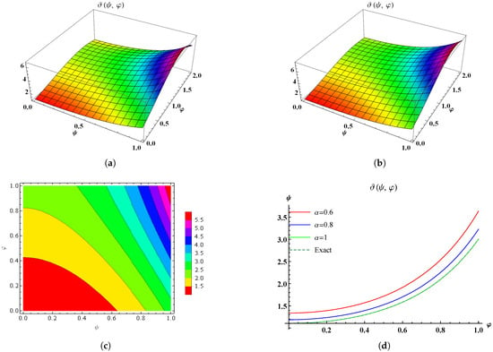
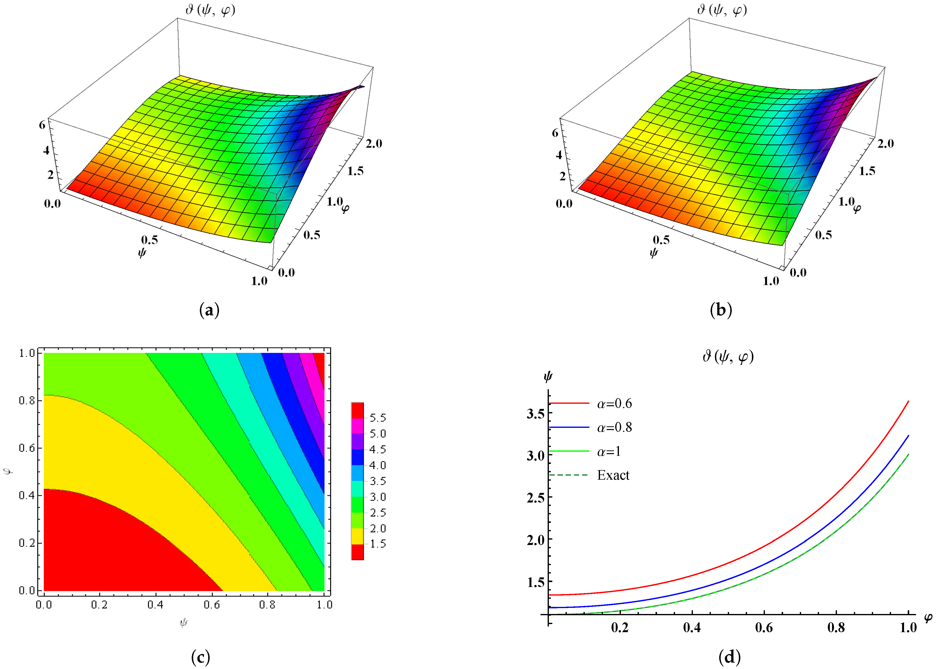
Figure 1a displays the physical behavior of the ET-HPM solution for a fractional order $\alpha =1$, whereas Figure 1b shows the physical behavior of the precise results including $0\le \psi \le 1$ and $0\le \phi \le 2$ for Problem 1. The 3-D graphical visuals show that both graphs are close and reveal the significance of our proposed scheme. Figure 1c demonstrates the contour plot, which examines the correlation across three variables on a single graph and the expression of $\psi$ and $\phi$ that gives the ideal results of $\vartheta (\psi ,\phi )$. The contour lines relate multiple combinations of the variables that generate similar parameters of $\vartheta (\psi ,\phi )$ at $0\le \psi \le 1$ and $0\le \phi \le 1$. Figure 1d depicts the error distribution of $\vartheta (\psi ,\phi )$ at $0\le \psi \le 1$ and $\phi =0.1$ with $\alpha =0.6$ (red), $\alpha =0.8$ (blue), and $\alpha =1$ (green) and the precise result (the dotted line). Table 1 shows the error distribution between the ET-HPM and precise results. The ET-HPM results are obtained at different fractional orders, such as $\alpha =0.4,0.6,0.8$, and 1. By increasing the parameter of the fractional order, our computed results become closer to the precise results.

Figure 1. The geometric layout of $\vartheta (\psi ,\phi )$. (a) The ET-HPM solution of $\vartheta (\psi ,\phi )$ at $\alpha =1$. (b) The precise solution of $\vartheta (\psi ,\phi )$. (c) A contour variation of $\vartheta (\psi ,\phi )$ at $\alpha =1$. (d) A visual variation across ET-HPM and precise results.

Table 1. A comparison of the exact and ET-HPM results of Problem 1 in Section 6.1 at different fractional orders.

$(\mathit{\psi },\mathit{\phi })$	ET-HPM	ET-HPM	ET-HPM	ET-HPM	Exact Results	Error Analysis
	$\mathit{\alpha }=\mathbf{0.4}$	$\mathit{\alpha }=\mathbf{0.6}$	$\mathit{\alpha }=\mathbf{0.8}$	$\mathit{\alpha }=\mathbf{1}$
(0.25, 0.01)	1.28334	1.14351	1.09367	1.07519	1.07519	00000
(0.50, 0.01)	1.54801	1.37933	1.31922	1.29693	1.29693	00000
(0.75, 0.01)	2.11588	1.88533	1.80316	1.77269	1.77269	00000
(1.00, 0.01)	3.27713	2.92005	2.79279	2.74560	2.7456	00000
(0.25, 0.03)	1.4286	1.22415	1.13634	1.09690	1.09690	00000
(0.50, 0.03)	1.72322	1.4766	1.37069	1.32312	1.32312	00000
(0.75, 0.03)	2.35536	2.01828	1.87351	1.80849	1.8085	0.00001
(1.00, 0.03)	3.64806	3.12597	2.90175	2.80104	2.80105	0.00001
(0.25, 0.05)	1.5301	1.28832	1.17646	1.11903	1.11905	0.00002
(0.50, 0.05)	1.84565	1.55401	1.41689	1.34980	1.34983	0.00003
(0.75, 0.05)	2.52271	2.12407	1.93666	1.84496	1.84500	0.00004
(1.00, 0.05)	3.90725	3.28983	2.99956	2.85753	2.85759	0.00004

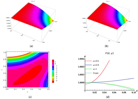
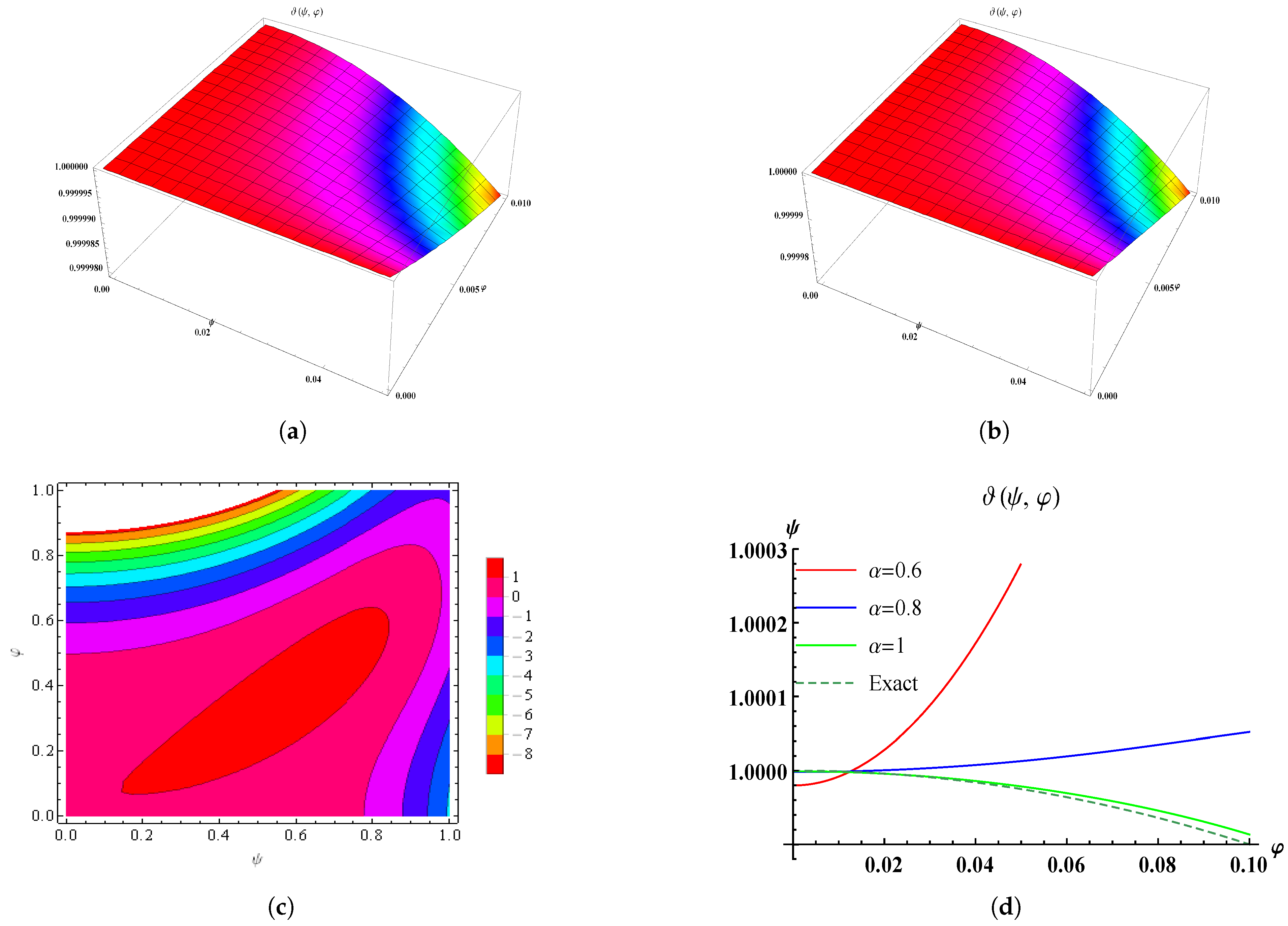
Similarly, we display the physical behavior of the ET-HPM solution for a fractional order $\alpha =1$ in Figure 2a, whereas Figure 2b shows precise results including $0\le \psi \le 0.05$ and $0\le \phi \le 0.01$ for Problem 2. The 3-D graphical visuals show that both graphs are close and reveal the significance of our proposed scheme. Figure 2c demonstrates the contour plot, which examines the correlation across three variables on a single graph and the expression of $\psi$ and $\phi$ that gives the ideal results of $\vartheta (\psi ,\phi )$. The contour lines relate multiple combinations of the variables that generate similar parameters of $\vartheta (\psi ,\phi )$ at $0\le \psi \le 1$ and $0\le \phi \le 1$. Figure 2d depicts the error distribution of $\vartheta (\psi ,\phi )$ at $0\le \psi \le 0.1$ and $\phi =0.01$ with $\alpha =0.6$ (red), $\alpha =0.8$ (blue), and $\alpha =1$ (green) and the precise result (the dotted line). Table 2 represents the error distribution between the ET-HPM and precise results. The ET-HPM results are derived at various fractional orders, such as $\alpha =0.4,0.6,0.8$, and 1. By extending the fractional-order value, we obtain results that are close to the precise results.

Figure 2. The geometric layout of $\vartheta (\psi ,\phi )$. (a) The ET-HPM solution of $\vartheta (\psi ,\phi )$ at $\alpha =1$. (b) The precise solution of $\vartheta (\psi ,\phi )$. (c) A contour variation of $\vartheta (\psi ,\phi )$ at $\alpha =1$. (d) A visual variation across ET-HPM and precise results.

Table 2. A comparison of the exact and ET-HPM results of Problem 2 in Section 6.2 at different fractional orders.

$(\mathit{\psi },\mathit{\phi })$	ET-HPM	ET-HPM	ET-HPM	ET-HPM	Exact Results	Error Analysis
	$\mathit{\alpha }=\mathbf{0.4}$	$\mathit{\alpha }=\mathbf{0.6}$	$\mathit{\alpha }=\mathbf{0.8}$	$\mathit{\alpha }=\mathbf{1}$
(0.1, 0.01)	1.00940	1.00118	1.00005	0.99991	0.99990	0.00001
(0.2, 0.01)	1.03743	1.00415	0.99979	0.99938	0.99960	0.00022
(0.3, 0.01)	1.07548	1.00293	0.99525	0.99594	0.99910	0.00316
(0.4, 0.01)	1.08962	0.97375	0.97084	0.97988	0.98840	0.00852
(0.1, 0.03)	1.01852	1.00388	1.00052	0.99984	0.99970	0.00014
(0.2, 0.03)	1.08700	1.01700	1.00200	0.99917	0.99880	0.00037
(0.3, 0.03)	1.19268	1.03293	1.00050	0.99557	0.99730	0.00173
(0.4, 0.03)	1.30197	1.02824	0.98064	0.97945	0.99520	0.01575
(0.1, 0.05)	1.01562	1.00498	1.00097	0.99984	0.99950	0.00034
(0.2, 0.05)	1.11876	1.02982	1.00535	0.99945	0.99800	0.00145
(0.3, 0.05)	1.28216	1.06541	1.00882	0.99639	0.99550	0.00089
(0.4, 0.05)	1.47214	1.08852	0.99616	0.98119	0.99200	0.01081

Contour graphics are an effective visualization tool for representing three-dimensional data in two dimensions. The contour graphs demonstrate the result $\vartheta (\psi ,\phi )$ of the time-fractional Emden–Fowler equation across a domain in the space $\psi$ and time $\phi$ planes. These graphical simulations are helpful in understanding the dynamic behavior of the obtained results. The contour lines depict the constant parameters of the results $\vartheta (\psi ,\phi )$, providing a visual representation of the solution’s evolution over space and time. Only three iterations are considered for analytical computation results. It is evident that the accuracy of the results can be significantly enhanced by incorporating additional parameters, and the errors will come closer to zero. By extending the value of $\alpha$, the nonlinearity impact is influenced, even though the wave amplitude decreases. We have observed that the ET-HPM is entirely designed for handling both linear and nonlinear time-fractional models.

8. Conclusions

In this paper, we successfully obtained the analytical solutions of linear and nonlinear time-fractional Emden–Fowler models via the ET-HPM strategy. Two numerical problems were adequately examined traditionally using this proposed approach. The fractional orders are introduced in Caputo form. Our proposed scheme shows excellence in obtaining iterative results that are very close to the precise solution. By simplifying the fractional problem in the transform domain, the ET-HPM can provide more valuable convergence aspects of the solution series. The suggested approach generates convergence series systems with simple identifiable variables without the need for linearization, interference, or restricting constraints. The analytical and visualized findings obtained by the recommended approach are considerably more appealing and effective in determining the solutions of time-fractional models. This approach has significant promise for solving fractional differential problems. We will consider expanding this scheme for real-life problems with larger dimensions to other fractal and fractional phenomena encountered in engineering and science trends in future work.

References

- AlBaidani, M.M.; Ganie, A.H.; Khan, A. Computational analysis of fractional-order KdV systems in the sense of the Caputo operator via a novel transform. Fractal Fract. 2023, 7, 812. [Google Scholar] [CrossRef] [Scilit]
- AlBaidani, M.M.; Aljuaydi, F.; Alharthi, N.; Khan, A.; Ganie, A.H. Study of fractional forced KdV equation with Caputo–Fabrizio and Atangana–Baleanu–Caputo differential operators. AIP Adv. 2024, 14, 015340. [Google Scholar] [CrossRef] [Scilit]
- Beghami, W.; Maayah, B.; Bushnaq, S.; Abu Arqub, O. The Laplace optimized decomposition method for solving systems of partial differential equations of fractional order. Int. J. Appl. Comput. Math. 2022, 8, 52. [Google Scholar] [CrossRef] [Scilit]
- Akram, M.; Ihsan, T.; Allahviranloo, T. Solving Pythagorean fuzzy fractional differential equations using Laplace transform. Granul. Comput. 2023, 8, 551–575. [Google Scholar] [CrossRef] [Scilit]
- Kilbas, A.A.; Srivastava, H.M.; Trujillo, J.J. Theory and Applications of Fractional Differential Equations; Elsevier: Amsterdam, The Netherlands, 2006. [Google Scholar]
- Miller, K.S.; Ross, B. An Introduction to the Fractional Calculus and Fractional Differential Equations; A Wiley: New York, NY, USA, 1993. [Google Scholar]
- Wu, G.C.; Shi, Y.G.; Wu, K.T. Adomian decomposition method and non-analytical solutions of fractional differential equations. Rom. J. Phys. 2011, 56, 873–880. [Google Scholar]
- Odibat, Z.; Momani, S.; Xu, H. A reliable algorithm of homotopy analysis method for solving nonlinear fractional differential equations. Appl. Math. Model. 2010, 34, 593–600. [Google Scholar] [CrossRef] [Scilit]
- Modanli, M.; Abdulazeez, S.T.; Husien, A.M. A residual power series method for solving pseudo hyperbolic partial differential equations with nonlocal conditions. Numer. Methods Partial. Differ. Equ. 2021, 37, 2235–2243. [Google Scholar] [CrossRef] [Scilit]
- Alomari, A. Homotopy-Sumudu transforms for solving system of fractional partial differential equations. Adv. Differ. Equ. 2020, 2020, 222. [Google Scholar] [CrossRef] [Scilit]
- Lane, H.J. On the theoretical temperature of the sun, under the hypothesis of a gaseous mass maintaining its volume by its internal heat, and depending on the laws of gases as known to terrestrial experiment. Am. J. Sci. 1870, 2, 57–74. [Google Scholar] [CrossRef] [Scilit]
- Mall, S.; Chakraverty, S. A novel Chebyshev neural network approach for solving singular arbitrary order Lane-Emden equation arising in astrophysics. Netw. Comput. Neural Syst. 2020, 31, 142–165. [Google Scholar] [CrossRef] [Scilit]
- Chowdhury, M.; Hashim, I. Solutions of Emden–Fowler equations by homotopy-perturbation method. Nonlinear Anal. Real World Appl. 2009, 10, 104–115. [Google Scholar] [CrossRef] [Scilit]
- Mall, S.; Chakraverty, S. Numerical solution of nonlinear singular initial value problems of Emden–Fowler type using Chebyshev Neural Network method. Neurocomputing 2015, 149, 975–982. [Google Scholar] [CrossRef] [Scilit]
- Syam, M.I. Analytical solution of the fractional initial Emden–Fowler equation using the fractional residual power series method. Int. J. Appl. Comput. Math. 2018, 4, 1–8. [Google Scholar] [CrossRef] [Scilit]
- Swati; Singh, K.; Verma, A.K.; Singh, M. Higher order Emden–Fowler type equations via uniform Haar Wavelet resolution technique. J. Comput. Appl. Math. 2020, 376, 112836. [Google Scholar] [CrossRef] [Scilit]
- Gul, H.; Ali, S.; Shah, K.; Muhammad, S.; Sitthiwirattham, T.; Chasreechai, S. Application of asymptotic homotopy perturbation method to fractional order partial differential equation. Symmetry 2021, 13, 2215. [Google Scholar] [CrossRef] [Scilit]
- He, J.H.; El-Dib, Y.O. Homotopy perturbation method with three expansions for Helmholtz-Fangzhu oscillator. Int. J. Mod. Phys. B 2021, 35, 2150244. [Google Scholar] [CrossRef] [Scilit]
- Kharrat, B.N.; Toma, G.A. Development of homotopy perturbation method for solving nonlinear algebraic equations. Int. J. Sci. Res. Math. Stat. Sci. 2020, 7, 47–50. [Google Scholar]
- Akter, M.T.; Chowdhury, M.M. Homotopy perturbation method for solving highly nonlinear reaction-diffusion-convection problem. Am. J. Math. Stat. 2019, 9, 136–141. [Google Scholar]
- Iqbal, S.; Javed, A. Application of optimal homotopy asymptotic method for the analytic solution of singular Lane–Emden type equation. Appl. Math. Comput. 2011, 217, 7753–7761. [Google Scholar] [CrossRef] [Scilit]
- He, J.H. Application of homotopy perturbation method to nonlinear wave equations. Chaos Solitons Fractals 2005, 26, 695–700. [Google Scholar] [CrossRef] [Scilit]
- Yıldırım, A.; Momani, S. Series solutions of a fractional oscillator by means of the homotopy perturbation method. Int. J. Comput. Math. 2010, 87, 1072–1082. [Google Scholar] [CrossRef] [Scilit]
- Ghoreishi, M.; Md, A.I.B.; Ismail. The homotopy perturbation method (HPM) for nonlinear parabolic equation with nonlocal boundary conditions. Appl. Math. Sci. 2011, 5, 113–123. [Google Scholar]
- Javeed, S.; Baleanu, D.; Waheed, A.; Shaukat Khan, M.; Affan, H. Analysis of homotopy perturbation method for solving fractional order differential equations. Mathematics 2019, 7, 40. [Google Scholar] [CrossRef] [Scilit]
- Khader, M. Introducing an efficient modification of the homotopy perturbation method by using Chebyshev polynomials. Arab J. Math. Sci. 2012, 18, 61–71. [Google Scholar] [CrossRef] [Scilit]
- Elzaki, T.M. The new integral transform Elzaki transform. Glob. J. Pure Appl. Math. 2011, 7, 57–64. [Google Scholar]
- Aggarwal, S.; Bhatnagar, K.; Dua, A. Dualities between Elzaki transform and some useful integral transforms. Int. J. Innov. Technol. Explor. Eng. 2019, 8, 4312–4318. [Google Scholar] [CrossRef] [Scilit]
- Jassim, H.K.; Shareef, M. On approximate solutions for fractional system of differential equations with Caputo-Fabrizio fractional operator. J. Math. Comput. Sci. 2021, 23, 58–66. [Google Scholar] [CrossRef] [Scilit]
- Mohamed, M.Z.; Yousif, M.; Hamza, A.E. Solving nonlinear fractional partial differential equations using the Elzaki transform method and the homotopy perturbation method. Abstr. Appl. Anal. 2022, 2022, 4743234. [Google Scholar] [CrossRef] [Scilit]
- Sedeeg, A.K.H. A coupling Elzaki transform and homotopy perturbation method for solving nonlinear fractional heat-like equations. Am. J. Math. Comput. Model. 2016, 1, 15–20. [Google Scholar]
- Liu, F.; Yang, L.; Nadeem, M. A new fractal transform for the approximate solution of Drinfeld–Sokolov–Wilson model with fractal derivatives. Fractals 2023, 31, 2350007. [Google Scholar] [CrossRef] [Scilit]
Disclaimer/Publisher’s Note: The statements, opinions and data contained in all publications are solely those of the individual author(s) and contributor(s) and not of MDPI and/or the editor(s). MDPI and/or the editor(s) disclaim responsibility for any injury to people or property resulting from any ideas, methods, instructions or products referred to in the content. |
© 2024 by the authors. Licensee MDPI, Basel, Switzerland. This article is an open access article distributed under the terms and conditions of the Creative Commons Attribution (CC BY) license (https://creativecommons.org/licenses/by/4.0/).