Abstract
This paper proposes a multifractal least squares support vector machine detrended fluctuation analysis (MF-LSSVM-DFA) model. The system is an extension of the traditional MF-DFA model. To address potential overfitting or underfitting caused by the fixed-order polynomial fitting in MF-DFA, LSSVM is employed as a superior alternative for fitting. This approach enhances model accuracy and adaptability, ensuring more reliable analysis results. We utilize the p model to construct a multiplicative cascade time series to evaluate the performance of MF-LSSVM-DFA, MF-DFA, and two other models that improve upon MF-DFA from recent studies. The results demonstrate that our proposed modified model yields generalized Hurst exponents and scaling exponents that align more closely with the analytical solutions, indicating superior correction effectiveness. In addition, we explore the sensitivity of MF-LSSVM-DFA to the overlapping window size s. We find that the sensitivity of our proposed model is less than that of MF-DFA. We find that when s exceeds the limited range of the traditional MF-DFA, and are closer than those obtained in MF-DFA when s is in a limited range. Meanwhile, we analyze the performances of the fitting of the two models and the results imply that MF-LSSVM-DFA achieves a better outstanding performance. In addition, we put the proposed MF-LSSVM-DFA into practice for applications in the medical field, and we found that MF-LSSVM-DFA improves the accuracy of ECG signal classification and the stability and robustness of the algorithm compared with MF-DFA. Finally, numerous image segmentation experiments are adopted to verify the effectiveness and robustness of our proposed method.
1. Introduction
Fractal theory has been an important basis for the research of the nonstationary and nonlinear time series since it was proposed by Mandelbrot. Many scholars utilized the fractal method to explore the complexity and systematic of the time series. Fractal theory has indeed played a significant role in natural sciences [1], material structure [2], and medicine [3], where it has been used for accurate EEG signal segmentation through fractal dimension analysis. Fractal theory provides unique tools and methodologies that aid in understanding and analyzing the complex phenomena and structures within these fields. Subsequently, in order to obtain a more detailed description of a fractal, it is necessary to add parameters that can describe different fractal subsets, so multifractal theory should be introduced, which is a research hotspot [4,5,6,7].
Based on extensive empirical research on Nile water flow, Hurst [8,9] proposed Rescaled Range Analysis (R/S) which is the most classic method to explore the long-memory nature of the time series. Due to the sensitivity of the outliers to (R/S), Peng et al. [10] proposed the detrended fluctuation analysis (DFA) method. However, regardless of R/S or DFA, they only work on the analysis of the single fractal features of the time series. They cannot describe the whole structure of the object. Therefore, Kantelhardt et al. [11] combined multifractal and DFA to construct the multifractal detrended fluctuation analysis (MF-DFA) which has been widely used in the multifractal nature of the time series [12].
Since the MF-DFA method has been put forward, it has shone in many fields. The MF-DFA method plays an important role in analyzing the one-dimensional sequences. In the financial field, MF-DFA can effectively analyze multifractal characteristics under different time scales. Thompson and Wilson [13] used MF-DFA to show the volatility clustering or other highly irregular behavior of the financial time series. The MF-DFA method is commonly used to examine the efficiency of the markets [14,15,16]. As well, MF-DFA can realize the effective analysis of social phenomena and events [17,18]. In addition, MF-DFA has been widely used in other sequence processing [19,20,21,22]. Wang et al. [23] applied MF-DFA to the classification of ECG signals. Cao et al. [24] used MF-DFA to extract the features of EEG signals and the proposed method can be helpful for the recognition of sudden pain. Yu et al. [25] investigated the daily rainfall time series in the Yangtze River basin. Except for one-dimensional time series, MF-DFA performs well in two-dimensional (2D) images. Many researchers have explored the 2D surfaces by using the MF-DFA method [26,27,28]. Wang et al. utilized MF-DFA for classifying 2D images, including magnetic resonance images [29] and retinal images [30]. Additionally, Shi et al. [31] applied MF-DFA for the segmentation of 2D images.
In order to enhance the performance of the MF-DFA model, many scholars have extended the model in different ways. Considering that the MF-DFA method is only used to study a single time series, Zhou [32] combined MF-DFA with DCCA, which is proposed by Podobnik and Stanley [33], to construct the MF-DCCA method which can explore the cross-correlation of two sets of sequences. However, the fitting in both MF-DFA and MF-DCCA is the polynomial fitting, indicating that inherent and polynomial trends cannot be completely eliminated [34]. Therefore, considering the sensitivity of DFA to trends, Xu et al. [35] proposed a smoothing algorithm based on the discrete Laplace transform to minimize the influence of exponential trends and distortion in the double log plots acquired by MF-DFA. Subsequently, the detrended moving average has been applied to two nonlinear time series. Nian and Fu [36] incorporated the extended self-similarity to construct a novel MF-DFA method, whose performance was more excellent than traditional MF-DFA.
The fitting method in the traditional MF-DFA model is the polynomial fit which is simple and easy to achieve. The polynomial fitting works well for small data and simple relationships. It is the foundation for many nonlinear models. However, the degree of the fitting needs to be determined manually, easily leading to underfitting or overfitting. The support vector machine (SVM), having excellent generalizability and robustness, is commonly used in classification, regression prediction, function approximation and time series prediction. The least squares support vector machine (LSSVM) is an extended form of SVM, which uses the least squares method to replace the quadratic optimization algorithm of SVM. LSSVM reduces the number of parameters, decreases the complexity of the algorithm and improves the efficiency of calculation by using the Lagrange function.
Considering the MF-DFA method is widely used to deal with the nonlinear and nonstationary time series and the degree of the polynomial fitting is fixed, indicating that the fitting method is destined to suffer from under-fitting or over-fitting; therefore, the LSSVM fit is used to replace the polynomial fit in this paper.
The paper is organized in the following manner. In Section 2, we introduce the generation method of multiplicative cascading constructed time series, and describe the algorithms of MF-DFA, LSSVM, and MF-LSSVM-DFA. We provide the performance of the MF-LSSVM-DFA method with numerical experiments in Section 3. In Section 4 we apply MF-LSSVM-DFA to the classification of EEG signals in the medical field. In Section 5 we apply the method proposed in this paper to image segmentation. Some conclusions are delivered in Section 6.
2. Methodology
All the computations are processed by using Matlab R2020a on an Intel(R) Core(TM) i5-7200U CPU @ 2.50 GHz processor.
2.1. Multifractal Detrended Fluctuation Analysis
Based on DFA, MF-DFA develops and it is important to explore the multifractal nature of non-stationary time series. The specific steps of the MF-DFA algorithm are given as follows:
Firstly, for the given time series . Therefore, we construct the cumulative summation sequence as follows:
in Equation (1), is the mean value of the sequence.
Secondly, fix the window size s, and we divide the new series into W non-overlapping windows. W equals which indicates the possibility of missing information. Therefore, we divide according to i from small to large and from large to small, respectively. Thus, a total of intervals are obtained.
Thirdly, apply the least squares method to finish the k-th polynomial fitting for the points in each interval :
The following step is to calculate the mean square error :
When ,
when ,
Afterwards, we can obtain the fluctuation function through the the function:
The wave function increases in a power-law relationship with the increase in s which can be marked as . is the generalized Hurst exponent and when q equals 2, is the standard Hurst exponent. If the original time series is a single fractal, the scaling exponents in all the intervals are consistent and is a constant which is independent from q. Otherwise, the original time series has a multifractal nature.
When the sequence has a multifractal nature, the scaling exponent is used to evaluate the degree of multifractality:
2.2. Least Square Support Vector Machine
SVM is a supervised learning model, usually used for pattern recognition, classification and regression analysis. Especially, the fitting accuracy of SVM is high which is suitable for small sample data. LSSVM, proposed by Suykens [37], adopted the least squares linear system as a loss function which decreases the complexity of calculation. In addition, when using the same kernel function, the parameter of LSSVM is one less than that of traditional SVM, implying that the operation speed is faster. The LSSVM model is given as follows.
Given a set of training samples , :
where represents the weight vector, is the nonlinear function that maps the input space to a high-dimensional feature space, and represents the bias.
According to the principle of risk minimization, the optimization function is given as follows:
Here, represents the regularization parameter and represents the random errors. The Lagrange multiplier method is adopted to solve the problem:
where is the Lagrange multiplier which is called support values.
According to optimization conditions, we can obtain:
solve the above differential equations, we can obtain:
The next step is to solve pairwise problems, which is similar to SVM, we do not conduct any calculations on and e.
with . Therefore, the model is as follows:
where is called the kernel function.
2.3. MF-LSSVM-DFA Model
As shown in Section 2.1, fitting is an important step. However, the fitting method adopted by the traditional MF-DFA needs to be further improved. Most time series are nonlinear, implying that using only one fitting method may lead to overfitting or underfitting of some segments. For example, we give a nonlinear time series in Figure 1.
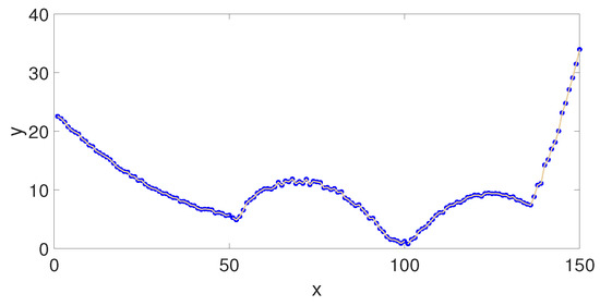
Figure 1.
A nonlinear time series.
We make a primary fitting, a secondary fitting and a tertiary fitting to the time series, respectively, which are shown in Figure 2.
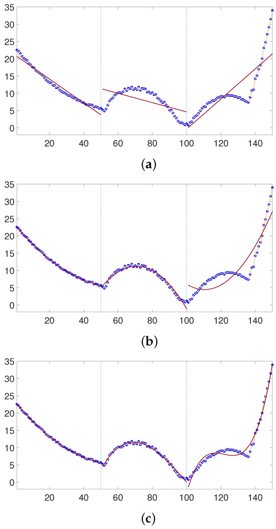
Figure 2.
Least squares fitting for different orders. The blue dots indicate the original data, and the red lines imply the fitting data. (a): The number of least-squares fitting for each segment is 1; (b): The number of least-squares fitting for each segment is 2; (c): The number of least-squares fits for each segment is 3.
It is obvious that when the fitting order equals 1, the second segment and the third segments are underfitting. When the number of the fit is 2, although the fitting results of the second segment are good, the first segment presents an overfitting performance and the last segment is underfitting. Figure 2c shows that when x belongs to [0, 100], the fit is overfitting. Therefore, when the fitting order of the nonlinear time series is single, the fitting performance of some segments of the time series is disappointing. Therefore, we replace the polynomial fitting function with LSSVM in the MF-DFA method. That is, replace Equation (2) with Equation (14). Equations (3) and (4) are updated as follows: When ,
when ,
2.4. Multiplicative Cascades Sequence
In this paper, we use multiplicative cascade sequences to measure the robustness of the proposed model. The multiplicative cascades time series is constructed by the p-model [38] due to its simple advantages [39]. The parameter p mainly determines the generated sequence. The initial time series has been generated as follows:
We define the length of the multiplicative cascades time series as N, where N equals , and is a positive integer. denotes the number of 1’s in binary form. In this paper, we set and the initial , which is shown in Figure 3.
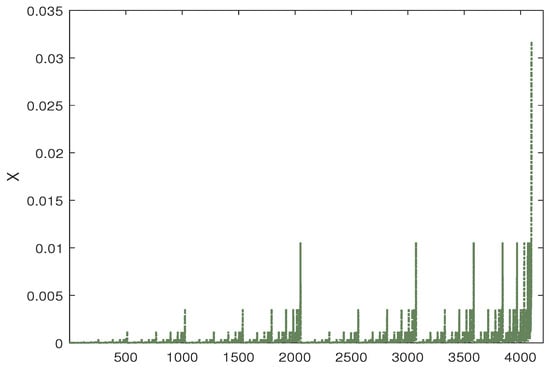
Figure 3.
Multiplicative cascade sequence constructed by p-model when and .
The analytic value of the scaling exponent and the generalized Hurst exponent can be calculated as follows.
3. Experiment Results
Several numerical experiments are performed to examine the robustness of the MF-LSSVM-FA method. We perform numerical experiments based on the p model. The related multifractal values are calculated according to q. We make q grow from −10 to 10 in intervals of 1. We obtain the values by using the MF-DFA. In addition, we calculate the analytical values which are all shown in Figure 4.
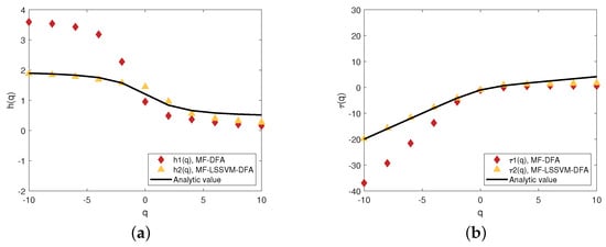
Figure 4.
Multifractal analysis of p model of (a) generalized Hurst exponent obtained by MF-DFA and MF-LSSVM-DFA and analytic value; (b) scaling exponent spectrum obtained by MF-DFA and MF-LSSVM-DFA and analytic value.
Figure 4, ⧫ represents the values calculated by MF-DFA, ▴ shows the values calculated by MF-LSSVM-DFA. The black line is the analytical value. It is obvious that when q ⩾ 0, the generalized Hurst exponent and the scaling exponent calculated by MF-LSSVM-DFA are closer to the analytical values than those calculated by MF-DFA. It is obvious that the generalized Hurst exponent and the scaling exponent calculated by the MF-LSSVM-DFA method are closer to the analtical solution than those calculated by the MF-DFA method, implying that the MF-LSSVM-DFA method performs better than the MF-DFA method.
In addition, we calculate the difference between the obtained Hurst exponent and the analytic value . We set and , where and represent the generalized Hurst exponents computed by MF-DFA and MF-LSSVM-DFA, respectively. Similar to and , we define and . and are the scaling exponents calculated by MF-DFA and MF-LSSVM-DFA, respectively. represents the analytic value. shows the difference between the Hurst exponent and the analytic value and so as . and exhibit the difference between the calculated value and the analytic value. The smaller the difference is, the more accurate the fitting is. The results can be seen in Figure 5.
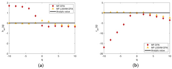
Figure 5.
Comparison of the difference between the calculated value and the analytic value: (a) the relative error of the Hurst exponent ; (b) the relative error of the scaling exponent . The fitting order adopted in MF-DFA is 2 and the size s belongs to [−10, 10].
The comparison of the fitting between MF-DFA and MF-LSSVM-DFA is shown in Figure 6. The red lines mean the fitting in MF-DFA and the fitting order is 2. The yellow lines show the LSSVM fitting in MF-LSSVM-DFA. For the nonlinear multiplicative cascade time series, the single polynomial fitting cannot fit each segment perfectly. Comparing the fitting effect of polynomial fitting and LSSVM fitting, i.e., the performance of the red and the yellow lines, it is obvious that the fitting performance of LSSVM is more detailed than polynomial fitting. Observing the red lines, the LSSVM fitting of each segment has a clear boundary, which seems to continue in the polynomial fitting. With different values of s, the difference of polynomial fitting is greater than that of LSSVM fitting.
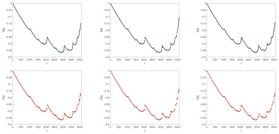
Figure 6.
Fitting forms of dispersion sequence. From top to bottom, the adopted models are MF-DFA (Black color) and MF-LSSVM-DFA (Red color), respectively. From left to right, s = 50, 60, 70, respectively. Fitting order is set by 2 in the MF-DFA.
3.1. Comparison between MF-LSSVM-DFA and MF-DFA with Different Fitting Order
Next, we compare the performance of different orders of the polynomial fitting and the performance of the MF-LSSVM-DFA method. We set the order of the polynomial fitting to be 1 and 3 which are shown in Figure 7 and Figure 8. It is obvious that regardless of whether the fitting order in MF-DFA is 1 or 3, the distance between the generalized Hurst exponent computed by MF-DFA is larger than that computed by MF-LSSVM-DFA. The calculated through the MF-LSSVM-DFA method almost coincides with the analytic value, indicating that the accuracy of the MF-LSSVM-DFA model is higher than that of the traditional MF-DFA model. We find that the fitting order in the MF-DFA model has an influence on the accuracy. Therefore, when using the MF-DFA model, suitable fitting order should be taken into account to decrease the difference between the calculated value and the analytic value. If the MF-LSSVM-DFA model is considered, it is unnecessary to consider the order problem, and the relative error is smaller than the traditional MF-DFA model.
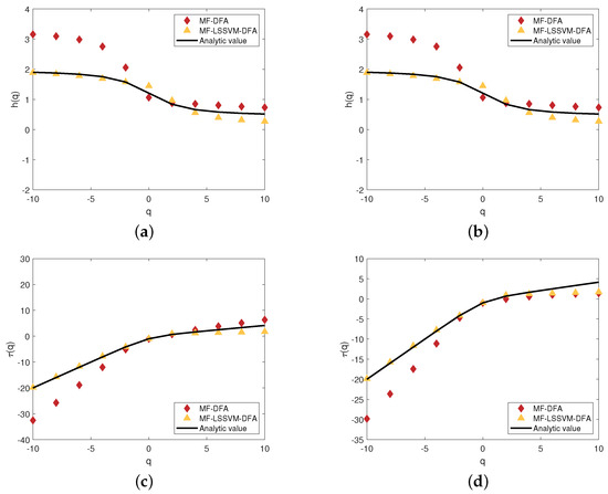
Figure 7.
Multifractal features of the MF-DFA model and MF-LSSVM-DFA model, the generalized Hurst exponent of (a,b) and the scaling exponent of (c,d). From left to right, the fitting order of the MF-DFA model is 1 and 3. The range of s is [50, 70].

Figure 8.
(a,b): The performance of the polynomial fitting and the fitting order is 1 and 3, respectively (Black color). (c): The performance of the LSSVM fitting. The range of s is [50, 70] (Red color).
Figure 8 exhibits the comparison of polynomial fitting and LSSVM fitting. Firstly, there is no need to consider the selection of the fitting order when using LSSVM fitting. Afterward, for most nonlinear and nonstationary time series, fixed fitting orders cannot perform excellently in each segment. Therefore, the overfitting or underfitting of some intervals is inevitable and unavoidable.
3.2. Multifractal Analysis with Differents
s in the proposed model is the size of the overlapping window. The traditional model is sensitive to the change of s. Therefore, we explore the sensitivity of the proposed modified model to the window size s.
Figure 9, Figure 10, Figure 11, Figure 12, Figure 13, Figure 14, Figure 15, Figure 16 and Figure 17 exhibit the fitting performance, the generalized Hurst exponent and the scaling exponent. In general, the distribution of the generalized Hurst exponent computed through the MF-LSSVM-DFA model is more compact than that calculated by the MF-DFA model. The Hurst exponents obtained from the MF-LSSVM-DFA model are around the analytic values.
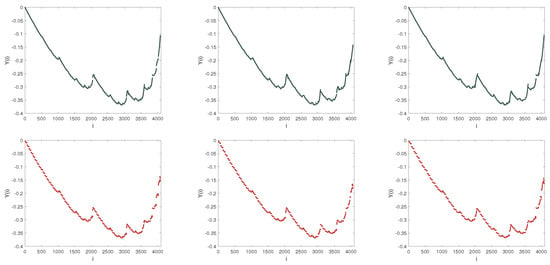
Figure 9.
Fitting forms of dispersion sequence. From top to bottom, the adopted models are MF-DFA (Black color) and MF-LSSVM-DFA (Red color), repectively. From left to right, s = 60, 70, 80, respectively. Fitting order is set by 2 in the MF-DFA.
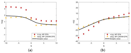
Figure 10.
The generalized Hurst exponent (a) and the scaling exponent (b) when
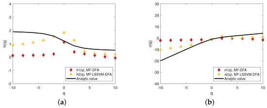
Figure 11.
The generalized Hurst exponent (a) and the scaling exponent (b) when
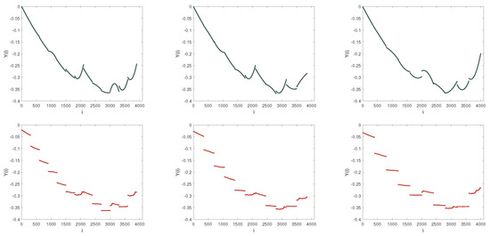
Figure 12.
Fitting forms of dispersion sequence. From top to bottom, the adopted models are MF-DFA (Black color) and MF-LSSVM-DFA (Red color), respectively. From left to right, s = 300, 350, 400, respectively. Fitting order is set by 2 in the MF-DFA.
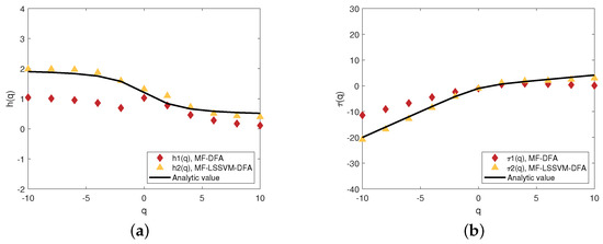
Figure 13.
The generalized Hurst exponent (a) and the scaling exponent (b) when .
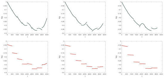
Figure 14.
Fitting forms of dispersion sequence. From top to bottom, the adopted models are MF-DFA (Black color) and MF-LSSVM-DFA (Red color), respectively. From left to right, s = 500, 550, 600, respectively. Fitting order is set by 2 in the MF-DFA.
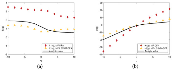
Figure 15.
The generalized Hurst exponent (a) and the scaling exponent (b) when
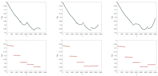
Figure 16.
Fitting forms of dispersion sequence. From top to bottom, the adopted models are MF-DFA (Black color) and MF-LSSVM-DFA (Red color), respectively. From left to right, s = 700, 750, 800, respectively. Fitting order is set by 2 in the MF-DFA.
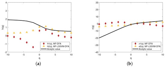
Figure 17.
The generalized Hurst exponent (a) and the scaling exponent (b) when
Figure 9 show the fitting conditions in the two models when , respectively. Figure 10 and Figure 11 present the generalized Hurst exponents and the scaling exponents when the range of s is small enough. We can find that when q is less than 0, is far from the analytic solution and is distributed around the analytic solution, especially in Figure 10a. In Figure 10b, the scaling exponent is almost completely consistent with the analytic value. Compared to , the difference between and the analytic value is large, which is over 10. When s grows, the difference between and the analytic solution becomes a little large. However, compared to Figure 10b, although becomes closer to the analytic value and becomes smaller, it still performs worse than . Therefore, when the segment size s is small, the MF-LSSVM-DFA model is excellent.
According to [40,41], in the traditional MF-DFA model, when the overlapping window size s is smaller than , it implies that the maximum s ought to be smaller than . Therefore, we explore the performance of the MF-LSSVM model when the segment size s is near and over the maximum value. The length of the multiplicative cascade sequence we use for numerical experiments is . Therefore, we select an interval [300, 400], in which the maximum value is a little less than , an interval [500, 600], in which the minimum value is a little greater than and an interval [700, 800], for which the minimum value is far larger than .
When the maximum s is slightly less than , that is, the range of s is a little smaller than the boundary, and the performance of the polynomial fitting is similar to before. The performance of LSSVM is quite different. Observing Figure 12, the segmentation of the LSSVM fit is more obvious. In Figure 12, we can see that the trends of the LSSVM fit are similar. On the opposite, in the interval [1500, 2000], when s equals 300 and 350, the opening is oriented upward. When s is 400, the opening is facing downward which is completely opposite to that when s is 300 and 350. Therefore, the LSSVM fit is more suitable for the nonlinear and nonstationary time series.
From Figure 13a,b, when , and are tightly distributed around the analytic value in both models. However, the generalized Hurst exponent and the scaling exponent calculated by MF-LSSVM-DFA are almost identical to the resolved values. Combining Figure 4, Figure 10, Figure 11 and Figure 15, we find that when the range of s is in the traditional specified range interval, the performances of both the MF-DFA model and the MF-LSSVM-DFA model are gratifying, and the MF-LSSVM-model is more outstanding.
Subsequently, we explore the performances of the MF-LSSVM-DFA model when the range outstrips the limit. Figure 14 and Figure 16 present the fitting in the two models when and when , respectively. Compared with the traditional MF-DFA model, the fitting trend is similar when s alters. The opening directions of the fitting in the similar interval are the opposite in MF-DFA when s changes. Figure 15 and Figure 17 exhibit the corresponding generalized Hurst exponents and the scaling exponents. In both Figure 15 and Figure 17, when the minimum s is greater than , the generalized Hurst exponent calculated by the proposed model is still closer to the analytic solution than that computed by the conventional MF-DFA, and so is the scaling exponent. In addition, we find that the scaling exponent is less sensitive to s than the generalized Hurst exponent. Especially when q is smaller than 0, alters from above the analytic solution to below the analytic solution and the difference between and the solution in Figure 15 is larger than that in Figure 17. Therefore, compared to the MF-DFA model, the proposed MF-LSSVM-DFA model is relatively less affected by s.
In addition, we calculate the difference between and the analytic value, and between and the analytic value for different ranges of s in Table 1 and Table 2, respectively. We calculate the average value of in each range. The results show that when the maximum s is smaller than , the average values of are almost around 0.1. When , the average value increases and surprisingly, the average value varies a little. When the minimum s becomes far larger than , becomes large and the average value when is far bigger than that when s in the former ranges. Comparing to Table 1, we find that the average value of is greater than that of when the range of s is the same. In addition, all the mean values of are under 1. However, when the minimum s is over , the mean value becomes larger and is over 1, indicating that there is a significant discrepancy between the calculated Hurst exponent and the analytic value. Therefore, our proposed model has a higher accuracy fit.

Table 1.
MF-DFA: based on different ranges of s.

Table 2.
MF-LSSVM-DFA: based on different ranges of s.
From Table 1 and Table 2, we find that when s belongs to [500, 600], is less than all the , denoting that even when the overlapping window size s is over , our proposed model still surpass the traditional MF-DFA model. Even when s belongs to [700, 800], is smaller than when s belongs to [50, 70]. At the same time, we explore whether the performance of the scaling exponent is consistent with the generalized Hurst exponent. We calculate the difference between the scaling exponent and the theoretic value. represents the absolute value of the difference calculated in MF-DFA, and shows the absolute value of the difference computed in MF-LSSVM-DFA. Therefore, we calculate the scaling exponent when s belongs to [500, 600] and [700, 800], respectively. Both the minimum values of the two selected ranges of s are over the length of the multiplicative cascade time series. In addition, we compute of the first five intervals of MF-DFA. The specific calculated results are shown in Table 3 and Table 4.

Table 3.
Comparison of the absolute value of the scaling exponent . The range of s in MF-LSSVM-DFA is determined by [500, 600].

Table 4.
Comparison of the absolute value of the scaling exponent . The range of s in MF-LSSVM-DFA is determined by [700, 800].
Figure 18 presents the distribution of the scaling exponents. From Figure 18a, we find that when q is the same, the scaling exponent obtained by MF-LSSVM-DFA when s is in [500, 600] is almost smaller than that calculated by MF-DFA, regardless of the interval of s. When the interval of s becomes larger where the minimum s is far larger than , and is still closer to the analytic value than when s belongs to [50, 70] and [300, 400]. Therefore, our proposed model has smaller restrictions on the window size s.
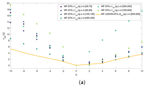
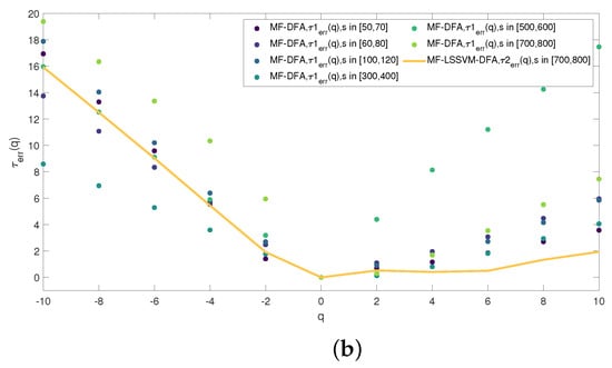
Figure 18.
The comparsison of the scaling exponent between MF-LSSVM-DFA and MF-DFA: (a) the range of s in MF-LSSVM-DFA is [500, 600] and (b) the range of s in MF-LSSVM-DFA is [700, 800].
To highlight the effectiveness of the proposed method, we compare it with existing improved MF-DFA methods. Yang et al. [42] addressed the potential presence of negative values in the original MF-DFA model by introducing sign retention to enhance performance, resulting in the sign retention model MF-S-DFA. Additionally, Wang et al. [43] proposed the MF-LF-DFA algorithm, which improves the performance of MF-DFA by reasonably setting the fitting order for different local intervals based on the fluctuation characteristics of the sequence. We calculate the Hurst values corresponding to different ranges of s. Let and denote the absolute differences between the results computed using MF-S-DFA and LF-MF-DFA methods and the analytical values, respectively. The final results are presented in Table 5. Comparing the averages of and in each range of s with those in Table 2, we find that the proposed method achieves better performance compared to the two existing improved MF-DFA methods.

Table 5.
MF-S-DFA;LF-MF-DFA: and based on different ranges of s.
Similarly, we calculate the variation in the differences between the scaling exponents of the two improved methods and the theoretical values across different ranges of s. Let and represent the absolute differences between the scaling exponents computed using MF-S-DFA and LF-MF-DFA methods and the theoretical values, respectively. We compare the values for s in the range [700, 800] with the and values computed for three different intervals, as presented in Table 6. From the results, we can see that our method is superior to improving MF-DFA.

Table 6.
Comparison of Proposed method, MF-S-DFA, and LF-MF-DFA of the absolute value of the scaling exponent .
4. MF-LSSVM-DFA for EEG Signal Classification
In this section, consider applying the proposed method to practical problems to verify if MF-LSSVM-DFA is more effective than traditional MF-DFA. EEG, as typical nonlinear signals, have been widely utilized by scholars for analytical research [44,45,46]. This section conducts an empirical analysis of EEG data from the Epilepsy Laboratory at the University of Bonn in Germany. The generalized Hurst exponent of the EEG signal is extracted using both the MF-LSSVM-DFA and MF-DFA models and then analyzed as input vectors for SVM to compare the effectiveness of the two methods.
The EEG signals are collected from the clinical EEG database of the Epilepsy Laboratory at the University of Bonn in Germany, which is a widely used public database. The dataset consists of EEG data from five healthy individuals and five patients with epileptic seizures. A total of 200 normal EEG signals and 300 arrhythmic signals are collected, all of which are single-channel datasets. Each sub-dataset contains 100 data segments, each lasting 23.6 s and comprising 4097 data points. The signal resolution is 12 bits, and the sampling frequency is 173.61 Hz.
For the EEG signal data, feature extraction is conducted using the MF-LSSVM-DFA algorithm and the MF-DFA algorithm. The fluctuation function order q ranges from −10 to 10. Non-overlapping windows are set with = 100 and = 190, with s increasing in steps of 9 from to . Using the MF-LSSVM-DFA algorithm for feature extraction, six generalized Hurst exponents are extracted to serve as input vectors for SVM classification. The extracted generalized Hurst exponents are depicted in Figure 19. From Figure 19, it can be seen that the EEG feature values extracted using the MF-LSSVM-DFA algorithm show a significant concentration trend for healthy individuals, with values primarily distributed in the range of 0.5 to 1.5. In contrast, the EEG feature values of epileptic patients exhibit a more dispersed distribution pattern. When the q value is the same, the generalized Hurst values of EEG for healthy individuals are generally higher than those of epileptic patients, indicating a significant difference in the complexity and regularity of their brain electrical activities.
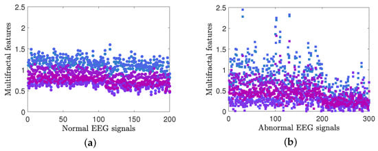
Figure 19.
(a,b) The generalized Hurst indices were extracted from EEG signal data based on MF-LSSVM-DFA for healthy persons and epileptic patients, respectively.
Furthermore, we utilize the obtained generalized Hurst exponents as input vectors for the SVM and feed them into the SVM classifier for further validation. We measure the classification using accuracy, sensitivity, and specificity. During classification, the SVM classifier employs a Gaussian kernel function, with 90% of the dataset used as the training set and 10% as the test set. We conduct classification validation using k-fold cross-validation with and compute each classification evaluation metric after 100 iterations. The results are depicted in Figure 20. Meanwhile, to validate the effectiveness of the MF-LSSVM-DFA algorithm, the traditional MF-DFA algorithm is employed for feature extraction from EEG signals and SVM is used for classification. The classification evaluation metrics including accuracy, sensitivity, and specificity can be found in Figure 21.

Figure 20.
Evaluation metrics for EEG signal classification based on the MF-LSSVM-DFA algorithm: (a) accuracy, (b) sensitivity, and (c) specificity.

Figure 21.
Evaluation metrics for EEG signal classification based on conventional MF-DFA algorithm: (a) accuracy; (b) sensitivity and (c) specificity.
In addition, the mean values of accuracy, sensitivity, and specificity after each iteration were calculated. These statistical results are summarized in Table 7. From the data in the Table 7, it can be observed that MF-LSSVM-DFA demonstrates higher accuracy, sensitivity, and specificity in the classification of electrocardiogram signals, proving its effectiveness and reliability in this field.

Table 7.
Evaluation metrics for two classification algorithms.
5. MF-LSSVM-DFA for Image Segmentation
In this section, to verify the effectiveness and robustness of our model, we apply our proposed model to image segmentation. The specific segmentation method can refer to [30]. We first perform segmentation on a simple model, and the segmentation results are shown in Figure 22. We observe that three different patterns reflect different segmentation states, indicating that our method can perform segmentation in different states for different targets. The results indicate that our proposed method can effectively perform edge segmentation on simple synthesized images.

Figure 22.
Simple synthesized image segmentation by MF-LSSVM-DFA method of (a) original image, (b) mask (White color), and (c) segmented state (Blue color).
Subsequently, we apply our proposed method to the segmentation of hyperspectral insulator images. Due to the low recognition of hyperspectral insulator images, effective segmentation of the image can demonstrate the advantages and efficiency of the MF-LSSVM-DFA method. The segmentation process of the hyperspectral insulator is shown in Figure 23.

Figure 23.
Hyperspectral insulator image segmentation by MF-LSSVM-DFA method of (a) original image, (b) mask (White color), and (c) segmented state (Blue color).
Finally, we analyze the image of the outdoor transmission tower, as shown in Figure 24a. Due to the complex background, multiple image components, and large gradients between pixels in outdoor images, the effective target localization of transmission equipment is more complex. We use the MF-LSSVM-DFA method for the target localization of such an image, as shown in Figure 24. We note that our proposed method can effectively segment transmission towers and their ancillary equipment in complex backgrounds.

Figure 24.
Outdoor transmission tower image segmentation by MF-LSSVM-DFA method of (a) original image, (b) mask (White color), and (c) segmented state (Blue color).
6. Conclusions
In this paper, the MF-LSSVM-DFA model was proposed as the modified model of the MF-DFA model. As an important step in the traditional MF-DFA model, the fitting method had a significant impact on MF-DFA. The polynomial fitting was adopted in the traditional MF-DFA model. However, although the order of the polynomial can be adjusted, there would still be overfitting or underfitting, or even both, in the fitting process. Considering the excellent performance of LSSVM, we replaced the polynomial fitting with LSSVM to construct the MF-LSSVM-DFA model. Subsequently, the multiplicative cascade time series was constructed for numerical experiments based on the p-model. The generalized Hurst exponent and the scaling exponent were used to examine the performance of MF-LSSVM-DFA. Firstly, we compared the performances between MF-LSSVM-DFA and MF-DFA, in which the order of the polynomial fitting is 2. Then, we varied the order of the polynomial fitting and the results showed that the proposed model performs more admirably than MF-DFA. Afterwards, we examined the sensitivity to the overlapping window size s of MF-LSSVM-DFA. When s was larger than , the increase in the variance of the difference between and the analytic value in the MF-LSSVM-DFA model was smaller than that in the MF-DFA model, denoting that the sensitivity of MF-LSSVM-DFA was smaller than MF-DFA. Thus, the universality of MF-LSSVM-DFA was stronger. Besides, we analyzed the performance of the fitting and we found that the fit was more detailed in MF-LSSVM-DFA than in MF-DFA, which indicated that our proposed model has better performance than the traditional MF-DFA. Finally, we put the proposed MF-LSSVM-DFA into practice, and the MF-LSSVM-DFA algorithm proposed in this paper performs better in practical applications compared with the traditional MF-DFA method. The improvement not only improved the accuracy of ECG signal classification but also enhanced the stability and robustness of the algorithm. By introducing LSSVM as an optimization tool, MF-LSSVM-DFA was able to deal with complex and nonlinear ECG signals more effectively, which provided a more accurate and reliable method for ECG signal analysis and heart disease diagnosis. Therefore, replacing the polynomial fit with the LSSVM fit could effectively improve the performance of MF-DFA. In addition, we employed the proposed method to segment the different category images such as the simple synthesized, hyperspectral insulator, and outdoor transmission tower images. The results validated the excellent performance of our model in image segmentation.
Author Contributions
Conceptualization, M.W. and W.J; methodology, J.W.; software, M.W.; validation, M.W., C.Z., K.Y., Y.Z., W.J. and J.W.; formal analysis, C.Z.; investigation, K.Y.; resources, C.Z.; data curation, Y.Z.; writing-original draft preparation, M.W.; writing-review and editing, J.W.; visualization, W.J.; supervision, J.W.; project administration, M.W. and J.W.; funding acquisition, M.W. and J.W. All authors have read and agreed to the published version of the manuscript.
Funding
The first author Minzhen Wang expresses thanks for the Management Technology Project of State Grid Liaoning Electric Power Co., LTD., project No. 2023YF-11. The corresponding author Jian Wang expresses thanks for the Natural Science Foundation of the Jiangsu Higher Education Institutions of China (Grant Nos. 22KJB110020) and supported by the Open Project of Center for Applied Mathematics of Jiangsu Province (Nanjing University of Information Science and Technology).
Institutional Review Board Statement
This article does not contain any studies with human participants or animals performed by any of the authors.
Informed Consent Statement
Informed consent was obtained from all individual participants included in the study.
Data Availability Statement
Data will be made available on request.
Conflicts of Interest
The authors Keyu Yue and Yu Zheng were employed by the State Grid Jilin Province Electric Power Co., LTD., Liaoyuan Power Supply Company. All authors declare that the research was conducted in the absence of any commercial or financial relationships that could be construed as a potential conflict of interest.
References
- Miao, T.; Chen, A.; Li, Z.; Liu, D.; Yu, B. Stress-dependent models for permeability and porosity of fractured rock based on fractal theory. Fractals 2023, 31, 2350093. [Google Scholar] [CrossRef]
- Wang, L.; Zeng, X.; Yang, H.; Lv, X.; Guo, F.; Shi, Y.; Hanif, A. Investigation and application of fractal theory in cement-based materials: A review. Fractal Fract. 2021, 5, 247. [Google Scholar] [CrossRef]
- Azami, H.; Bozorgtabar, B.; Shiroie, M. Automatic signal segmentation using the fractal dimension and weighted moving average filter. J. Electr. Comput. Sci. 2011, 11, 8–15. [Google Scholar]
- Sun, L.; Zhu, L.; Stephenson, A.; Wang, J. Measuring and forecasting the volatility of USD/CNY exchange rate with multi-fractal theory. Soft Comput. 2018, 22, 5395–5406. [Google Scholar] [CrossRef]
- Gosciniak, I. Semi-multifractal optimization algorithm. Soft Comput. 2019, 23, 1529–1539. [Google Scholar] [CrossRef]
- Achour, R.; Li, Z.; Selmi, B.; Wang, T. A multifractal formalism for new general fractal measures. Chaos Solitons Fractals 2024, 181, 114655. [Google Scholar] [CrossRef]
- Gu, G.F.; Zhou, W.X. Detrending moving average algorithm for multifractals. Phys. Rev. E 2010, 82, 011136. [Google Scholar] [CrossRef]
- Hurst, H.E. Long-term storage capacity of reservoirs. Trans. ASCE 1951, 116, 770–799. [Google Scholar] [CrossRef]
- Hurst, H.E. A suggested statistical model of some time series which occur in nature. Nature 1957, 180, 494. [Google Scholar] [CrossRef]
- Peng, C.K.; Buldyrev, S.V.; Havlin, S.; Simons, M.; Stanley, H.E.; Goldberger, A.L. Mosaic organization of DNA nucleotides. Phys. Rev. E 1994, 49, 1685. [Google Scholar] [CrossRef]
- Kantelhardt, J.W.; Zschiegner, S.A.; Koscielny-Bunde, E.; Havlin, S.; Bunde, A.; Stanley, H.E. Multifractal detrended fluctuation analysis of nonstationary time series. Physica A 2002, 316, 87–114. [Google Scholar] [CrossRef]
- Rak, R.; Kwapień, J.; Oświȩcimka, P.; Ziȩba, P.; Drożdż, S. Universal features of mountain ridge networks on Earth. J. Complex Netw. 2020, 8, cnz017. [Google Scholar] [CrossRef]
- Thompson, J.R.; Wilson, J.R. Multifractal detrended fluctuation analysis: Practical applications to financial time series. Math. Comput. Simul. 2016, 126, 63–88. [Google Scholar] [CrossRef]
- Yan, R.; Yue, D.; Chen, X.; Wu, X. Non-linear characterization and trend identification of liquidity in China’s new OTC stock market based on multifractal detrended fluctuation analysis. Chaos Solitons Fractals 2020, 139, 110063. [Google Scholar] [CrossRef]
- Fernandes, L.H.; Silva, J.W.; de Araujo, F.H. Multifractal risk measures by macroeconophysics perspective: The case of brazilian inflation dynamics. Chaos Solitons Fractals 2022, 158, 112052. [Google Scholar] [CrossRef]
- Ameer, S.; Nor, S.M.; Ali, S.; Zawawi, N.H.M. The Impact of COVID-19 on BRICS and MSCI Emerging Markets Efficiency: Evidence from MF-DFA. Fractal Fract. 2023, 7, 519. [Google Scholar] [CrossRef]
- Schadner, W. US Politics from a multifractal perspective. Chaos Solitons Fractals 2022, 155, 111677. [Google Scholar] [CrossRef]
- Wang, J.; Jiang, W.; Wu, X.; Yang, M.; Shao, W. Role of vaccine in fighting the variants of COVID-19. Chaos Solitons Fractals 2023, 168, 113159. [Google Scholar] [CrossRef] [PubMed]
- Xu, M.; Shang, P.; Xia, J. Traffic signals analysis using qSDiff and qHDiff with surrogate data. Commun. Nonlinear Sci. Numer. Simul. 2015, 28, 98–108. [Google Scholar] [CrossRef]
- Wang, F.; Fan, Q. Coupling correlation detrended analysis for multiple nonstationary series. Commun. Nonlinear Sci. Numer. Simul. 2021, 94, 105579. [Google Scholar] [CrossRef]
- Urda-Benitez, R.D.; Castro-Ospina, A.E.; Orozco-Duque, A. Characterization and classification of intracardiac atrial fibrillation signals using the time-singularity multifractal spectrum distribution. Commun. Nonlinear Sci. Numer. Simul. 2021, 96, 105675. [Google Scholar] [CrossRef]
- Sankaran, A.; Plocoste, T.; Geetha Raveendran Nair, A.N.; Mohan, M.G. Unravelling the Fractal Complexity of Temperature Datasets across Indian Mainland. Fractal Fract. 2024, 8, 241. [Google Scholar] [CrossRef]
- Wang, J.; Shao, W.; Kim, J. Ecg classification comparison between mf-dfa and mf-dxa. Fractals 2021, 29, 2150029. [Google Scholar] [CrossRef]
- Cao, T.; Wang, Q.; Liu, D.; Sun, J.; Bai, O. Resting state EEG-based sudden pain recognition method and experimental study. Biomed. Signal Process. Control 2020, 59, 101925. [Google Scholar] [CrossRef]
- Yu, Z.G.; Leung, Y.; Chen, Y.D.; Zhang, Q.; Anh, V.; Zhou, Y. Multifractal analyses of daily rainfall time series in Pearl River basin of China. Physica A 2014, 405, 193–202. [Google Scholar] [CrossRef]
- Yadav, R.; Dwivedi, S.; Mittal, A.; Kumar, M.; Pandey, A. Fractal and multifractal analysis of LiF thin film surface. Appl. Surf. Sci. 2012, 261, 547–553. [Google Scholar] [CrossRef]
- Wang, F.; Liao, D.W.; Li, J.W.; Liao, G.P. Two-dimensional multifractal detrended fluctuation analysis for plant identification. Plant Methods 2015, 11, 12. [Google Scholar] [CrossRef]
- Wang, F.; Fan, Q.; Stanley, H.E. Multiscale multifractal detrended-fluctuation analysis of two-dimensional surfaces. Phys. Rev. E 2016, 93, 042213. [Google Scholar] [CrossRef]
- Wang, J.; Shao, W.; Kim, J. Automated classification for brain MRIs based on 2D MF-DFA method. Fractals 2020, 28, 2050109. [Google Scholar] [CrossRef]
- Wang, J.; Shao, W.; Kim, J. Combining MF-DFA and LSSVM for retina images classification. Biomed. Signal Process. Control 2020, 60, 101943. [Google Scholar] [CrossRef]
- Shi, W.; Zou, R.B.; Wang, F.; Su, L. A new image segmentation method based on multifractal detrended moving average analysis. Phys. Stat. Mech. Its Appl. 2015, 432, 197–205. [Google Scholar] [CrossRef]
- Zhou, W.X. Multifractal detrended cross-correlation analysis for two nonstationary signals. Phys. Rev. E 2008, 77, 066211. [Google Scholar] [CrossRef]
- Podobnik, B.; Stanley, H.E. Detrended cross-correlation analysis: A new method for analyzing two nonstationary time series. Phys. Rev. Lett. 2008, 100, 084102. [Google Scholar] [CrossRef]
- Zhang, X.; Zhu, Y.; Yang, L. Multifractal detrended cross-correlations between Chinese stock market and three stock markets in The Belt and Road Initiative. Physica A 2018, 503, 105–115. [Google Scholar] [CrossRef]
- Xu, N.; Shang, P.; Kamae, S. Minimizing the effect of exponential trends in detrended fluctuation analysis. Chaos Solitons Fractals 2009, 41, 311–316. [Google Scholar] [CrossRef]
- Nian, D.; Fu, Z. Extended self-similarity based multi-fractal detrended fluctuation analysis: A novel multi-fractal quantifying method. Commun. Nonlinear Sci. Numer. Simul. 2019, 67, 568–576. [Google Scholar] [CrossRef]
- Suykens, J.A.; Lukas, L.; Van Dooren, P.; De Moor, B.; Vandewalle, J. Least squares support vector machine classifiers: A large scale algorithm. Eur. Conf. Circuit Theory Des. ECCTD 1999, 99, 839–842. [Google Scholar]
- Schertzer, D.; Lovejoy, S.; Schmitt, F.; Chigirinskaya, Y.; Marsan, D. Multifractal cascade dynamics and turbulent intermittency. Fractals 1997, 5, 427–471. [Google Scholar] [CrossRef]
- Meneveau, C.; Sreenivasan, K. Simple multifractal cascade model for fully developed turbulence. Phys. Rev. Lett. 1987, 59, 1424. [Google Scholar] [CrossRef]
- Kantelhardt, J. Multifractal deterended fluctuation analysis of nonstationary time series. Physica 2002, 316, 81–91. [Google Scholar]
- Ihlen, E. Introduction to multifractal detrended fluctuation analysis in Matlab. Front Physiol. 2012, 3, 141. [Google Scholar] [CrossRef] [PubMed]
- Yang, M.; Zhang, Y.; Wang, J. Sign Retention in Classical MF-DFA. Fractal Fract. 2022, 6, 365. [Google Scholar] [CrossRef]
- Wang, J.; Huang, M.; Wu, X.; Kim, J. A local fitting based multifractal detrend fluctuation analysis method. Phys. Stat. Mech. Its Appl. 2023, 611, 128476. [Google Scholar] [CrossRef]
- Azami, H.; Abásolo, D.; Simons, S.; Escudero, J. Univariate and Multivariate Generalized Multiscale Entropy to Characterise EEG Signals in Alzheimer’s Disease. Entropy 2017, 19, 31. [Google Scholar] [CrossRef]
- Chen, D.; Huang, H.; Bao, X.; Pan, J.; Li, Y. An EEG-based attention recognition method: Fusion of time domain, frequency domain, and non-linear dynamics features. Front. Neurosci. 2023, 17, 1194554. [Google Scholar] [CrossRef]
- Djemili, R.; Djemili, I. Nonlinear and chaos features over EMD/VMD decomposition methods for ictal EEG signals detection. Comput. Methods Biomech. Biomed. Eng. 2023, 1–20. [Google Scholar] [CrossRef]
Disclaimer/Publisher’s Note: The statements, opinions and data contained in all publications are solely those of the individual author(s) and contributor(s) and not of MDPI and/or the editor(s). MDPI and/or the editor(s) disclaim responsibility for any injury to people or property resulting from any ideas, methods, instructions or products referred to in the content. |
© 2024 by the authors. Licensee MDPI, Basel, Switzerland. This article is an open access article distributed under the terms and conditions of the Creative Commons Attribution (CC BY) license (https://creativecommons.org/licenses/by/4.0/).