Abstract
The intricacy and fractal properties of human DNA sequences are examined in this work. The core of this study is to discern whether complete DNA sequences present distinct complexity and fractal attributes compared with sequences containing exclusively exon regions. In this regard, the entire base pair sequences of DNA are extracted from the NCBI (National Center for Biotechnology Information) database. In order to create a time series representation for the base pair sequence , we use the Chaos Game Representation (CGR) approach and a mapping rule f, which enables us to apply the metric known as the Complexity–Entropy Plane (CEP) and multifractal detrended fluctuation analysis (MF-DFA). To carry out our investigation, we divided human DNA into two groups: the first is composed of the 24 chromosomes, which comprises all the base pairs that form the DNA sequence, and another group that also includes the 24 chromosomes, but the DNA sequences rely only on the exons’ presence. The results show that both sets provide fractal patterns in their structure, as obtained by the CGR approach. Complete DNA sequences show a sharper visual fractal pattern than sequences composed only of exons. Moreover, the sequences occupy distinct areas of the complexity–entropy plane, and the complete DNA sequences lead to greater statistical complexity and lower entropy than the exon sequences. Also, we observed that different fractal parameters between chromosomes indicate diversity in genomic sequences. All these results occur in different scales for all chromosomes.
1. Introduction
The emergence of high-throughput DNA sequencing technologies has revolutionized our understanding of the genetic foundations of life DNA sequences serve as the fundamental instructions for biological processes, providing insight into genetic variations, functional components, and evolutionary connections [,,,,]. To unlock the intricate code hidden within DNA, an array of computational techniques have been harnessed [,,,]. Other approaches involving generalized entropies investigated human DNA sequences and other living organisms [,]. These methodologies collectively enable the unveiling of hidden genetic patterns and deciphering the complex relationships that govern DNA’s role in shaping life’s diversity and complexity.
The term fractal geometry was coined initially by Mandelbrot in 1957 when he described the geometry of turbulence in fluids []. In a general way, fractal geometry is the systematic study of irregular shapes found in both mathematics and nature, where each small part is similar to its magnified image, and this similarity repeats across different scales. Fractals are characterized by a power law within the magnification process, with the same exponent related to the fractal dimension remaining constant even as the scale changes. If the exponent varies with the scale, we have a multifractal object with multiple fractal dimensions. The concept of multifractals was initially introduced in Frisch and Paris’s work in 1985 [], which built upon B. Mandelbrot’s earlier research in the 1970s []. This work popularized the term “multifractal analysis” among mathematicians and physicists. More specifically, from a mathematical standpoint, multifractal analysis refers to a technique used to precisely characterize the heterogeneity in the distribution of a set of measurements in a metric space at small scales [,,,]. This analysis aims to express the dimension of the set of measurements in terms of the Legendre transformation of a free energy function, drawing an analogy with thermodynamic theory. In mathematical analysis, the multifractal formalism is deemed applicable to a given set if the Legendre transform of its free energy yields the Hausdorff dimension of the set of measures of the local Hölder exponent of []. Historically, multifractal analysis relied on Mandelbrot’s box method, which was described in his book from the 1970s. This involved using boxes in a metric space entirely separate from geometry []. However, the mathematician Olsen sought to replace this approach with a more mathematically significant formalism within geometric measurement theory [], which is now widely used. Regardless of whether boxes are used, this formalism has been proven valid when an auxiliary measure, known as the Gibbs measure, is present []. Later, it was discovered that this formalism is valid under Olsen’s Hausdorff-like model, where the multifractal measure is positive [,]. Even today, new proofs of theorems on multifractal formalism are being explored in the field of mathematics [].
Among these methodologies, Chaos Game Representation (CGR) has emerged as a powerful instrument for analyzing and visualizing DNA or protein sequences [,,]. The CGR visually represents the distribution patterns of nitrogenous bases in genomic sequences. It highlights the structure and organization of sequences in an intuitive and accessible way [].
Another essential tool, the complexity–entropy causality plane, introduced in ref. [], has become a significant metric for quantifying the intricate structural properties of DNA sequences []. The complexity–entropy plane (CEP) allows the assessment of statistical complexity in time series data, particularly in DNA sequences, studying its behavior in phase space. It involves the creation of a two-dimensional plane and the mapping of DNA sequences onto it. The CEP approach then measures the entropy of this plane, which captures the system’s inherent structural properties and unpredictability. Higher CEP values indicate a higher level of sophistication and the presence of intricate fractal patterns within the DNA sequences. By employing CEP, researchers gain insight into the complex organizational characteristics of time series and can uncover hidden patterns and structural properties that may not be apparent from a straightforward examination of the sequences themselves [,,].
On the other hand, multifractal detrended fluctuation analysis (MF-DFA) is a technique used to study the complexity of time series [,,]. By applying fractal concepts, MF-DFA helps identify complex and heterogeneous patterns in time series and is widely used in fields such as physics, biology, and finance [,,,]. The method provides information about the multifractal distribution of fluctuations at different scales, revealing the intrinsic complexity of the data.
The analysis methods used in this study—CGR, CEP, and MF-DFA—are complementary in providing different perspectives on the properties of genomic sequences. While CGR offers a detailed visual representation of the distribution patterns of nitrogenous bases, CEP provides a quantitative analysis of the statistical complexity and entropy of the sequence. On the other hand, MF-DFA investigates the multifractal characteristics of sequences, revealing complex fluctuation patterns at different scales. By combining these methods, we can obtain a more complete and comprehensive understanding of genomic sequence structure, organization, and dynamics.
In DNA sequences, exons are the coding segments and keystones of genetics, housing the instructions for protein synthesis—the bedrock of cellular activities [,]. In contrast, introns, the noncoding stretches interwoven between exons, extend their significance beyond a mere genomic “spacer” [,,,,]. Introns are increasingly recognized for their involvement in gene regulation, alternative splicing, and even potential evolutionary innovation [,].
Here, we comprehensively investigate the characteristics of DNA sequences. The main aim is to discern whether complete DNA sequences exhibit distinct complexity and fractal attributes compared with sequences that contain only exon regions. Base pair sequences are used from the NCBI database in this regard []. We apply the Chaos Game Representation (CGR) approach and a mapping rule f to create a time series representation of the base pair sequence , allowing the application of the metric known as the complexity–entropy plane (CEP).
2. Theoretical Background
2.1. Chaos Game Representation
By applying the concepts of chaotic dynamics to the construction of an image of a gene sequence, the Chaos Game Representation (CGR) technique, as proposed by Jeffrey [], reveals patterns at both the local and global levels. This technique is based on chaotic dynamics and produces an image of the gene sequence that displays local and global patterns. Mathematically, the chaos game is described as an iterative function system (IFS) that allows representing a DNA sequence graphically in the form of an image.
CGR is significant in assessing the prevalence of k-mers within nucleotide sequences, with k being an adaptable integer of your choice. Each k-mer corresponds to a distinct sequence of length k from the DNA sequence, which facilitates the identification of specific regions within biomolecules such as DNA (for gene prediction) or proteins []. In the scientific realm, this technique is recognized as Frequency Chaos Game Representation (FCGR), enabling the visualization of k-mer frequencies in a given sequence through an image format. In this imagery, each pixel corresponds to a distinct k-mer []. The expansion of CGR to FCGR has ushered in novel approaches for sequence comparison and phylogenetic analysis [,,].
Visually, the construction of the FCGR for a k-mer can be achieved recursively through the following steps: for each nucleotide sequence letter, a box is subdivided into four quadrants: A occupies the upper left corner, T is placed in the lower right corner, G in the upper right corner, and C in the lower left corner, as illustrated in Figure 1. The frequency of monomers in each quadrant is assessed by the FCGR, which then assigns a grayscale value according to their relative occurrence. Typically, a darker quadrant signifies a higher frequency of occurrence, while a lighter shade suggests the opposite. This depiction is specifically related to .
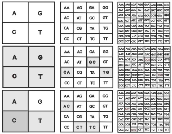
Figure 1.
Quadrants in FCGR at different pixelation levels k, where each quadrant uniquely corresponds to a specific string of length k. (Left column) . (Middle column) . (Right column) (Top row). FCGR for the “TGCA” sequence is shown in the middle line. The “ACTC” sequence is represented on the bottom line.
For instance, in the sequence “TGCA”, each quadrant receives an equal gray level, denoting a point within each quadrant. On the other hand, if we were to follow a different sequence, such as “ACTC”, we would see two points in the C quadrant, one in the A quadrant, one in the T quadrant, and none in the G quadrant. As a result, as shown in Figure 1, the grayscale intensity of the C quadrant is double that of the T and A quadrants, although the G quadrant stays white.
The FCGR for dimers, achieved with a pixelization level of , is generated through a process where each quadrant is further divided into four analogous subquadrants. This division is depicted in the top-middle row of Figure 1. Within a given quadrant, these four subquadrants encompass sequences that conclude with a specific dimer and only vary in the last nucleotide. Like in the monomer case, the frequencies within each subquadrant are computed and exhibited by varying the gray intensity levels. For example, in the scenarios of the sequences “TGCA” and “ACTC”, the FCGR tables for are portrayed in the middle column, middle row, and bottom row of Figure 1, respectively.
In the right column of Figure 1, the representation corresponds to: TGC, GCA for subsequence “TGCA”. For the “ACTC” subsequence: CTC and ACT. Since they all appear in the series at the same frequency, they have the same degree of gray, while the other representations are blank because they do not exist in the sequence.
Generally, to obtain points representing oligonucleotides of length k, we continue the above procedure until the pixelization level of k is desired. In this progression, the size of the box grows exponentially. For instance, when considering tetramers (), the resulting image will comprise boxes, each symbolizing a quartet of base pairs. The frequency of these quartets is also visually depicted through the color of the boxes, ranging from white (indicating the absence of the tetramer in the sequence) to black (denoting a widespread tetramer occurrence). Through the FCGR, nucleotide sequences become amenable to an entirely new suite of statistical analysis tools and facilitate the application of machine learning methodologies (See [] and references therein).
Global Distance
The distance between the genomic signatures of two DNA sequences is essential in evaluating their differences. Such a distance measure can be used, for example, in phylogenetic analysis. Several similarity measures can be used to compare two sequences []. For a given scale k, ref. [] suggests utilizing FCGR to calculate the dissimilarity, , between two DNA sequences. To perform this, we use the following formulas to obtain the global distance d between two FCGR of two DNA sequences.
where the values of and represent each k-mer’s frequency of occurrence in the first and second sequences, respectively. The is a kind of “normalization factor”, and are, respectively, a mean of frequency in the first and second sequence, and and are a kind of variance between the distribution. Finally, is the Pearson correlation coefficient modified. For example, consider the FCGR of two sequences for . We obtain the dimers AA, AC, AG, AT, …, TA, TC, TG, and TT for the two sequences in this configuration. The values and are the frequency of the 16 dimers of the first and second sequences, respectively.
The alteration to Pearson’s conventional definition involves incorporating a weighted variance, represented by the frequency . The essential advantage of employing this modified Pearson coefficient definition, as opposed to the other distance metrics, lies in the proportional significance assigned to each quadrant, in accordance with the represented oligomer’s frequency. By [], the global distance is defined:
Its value ranges from 0 to 2. The precise resemblance between the sequences is represented by null values of d, while values larger than one would indicate correlation coefficients of negative value.
2.2. Times Series and Fractal Theory
The four nitrogenous bases of DNA, which are also known as G, C, A, and T, are Guanine, Cytosine, Adenine, and Thymine. To use them in our analysis tools, we first convert the DNA sequence into a numerical sequence using a mapping rule f, where , , , and are the formal definitions of the mapping. As a result, we obtain as a sequence of values, where . The values of are cumulatively added to create our time series . There will be a value matching a temporal measurement t for each cumulative sum value. Ref. [] was the first publication to employ this mapping rule.
Formally, the time series consists of the sum of the elements of .
This definition of f allows us to distinguish purines and pyrimidines. We emphasize that alternative orders can be chosen to replace bases A, C, G, and T, such as Keto and GC coding [].
2.3. Ordinal Patterns
An advanced method that captures the dynamics of time series in great detail is the use of ordinal pattern algorithms. Using this method, a time series is converted into a series of rankings or patterns, each of which precisely reflects the order of values within a given data point window. This method’s strength is its capacity to reveal the minute details inside dynamic systems using metrics like the complexity–entropy plane and permutation entropy [,,,].
The principles behind this approach were first presented by Bandt and Pompe in 2002 [] as a reliable and computationally efficient way to measure complexity in time series data. At the core of this method lies the notion of measuring complexity through Shannon entropy. The probability distribution linked to these ordinal patterns is meticulously examined and extracted through partitions of the original time series using the Bandt–Pompe symbolization approach.
Assume that we perform N observations in the time series . The series is divided into nonoverlapping divisions (or partitions), with time separating the items. We acquire the partitions set for a given and . The index of the partition is denoted by p.
The components inside each division are then put in ascending order. To achieve this, we evaluate the permutation for each partition indicated by . This permutation effectively sorts the elements within in ascending order. Applying this step-by-step process to every data partition results in a symbolic sequence called , where . We suggest consulting the refs. [,,] for additional information about this technique.
The ordinal probability distribution is the relative frequency of all possible permutations within the symbolic sequence, given by
where represents each of the different ordinal patterns.
Complexity–Entropy Plane
The ordinal probability distribution is a fundamental component in the computation of the Shannon entropy of permutations. By analyzing the frequency and occurrence of different ordinal patterns within a time series, this distribution provides valuable insights into the underlying structure and dynamics of the data. The Shannon entropy, derived from this ordinal probability distribution , quantifies the level of uncertainty or randomness present in the arrangement of ordinal patterns
A higher Shannon entropy implies a more diverse and intricate pattern distribution, indicating greater complexity and potentially revealing important characteristics of the system generating the time series. In particular, randomness is indicated by , whereas more regular dynamics are indicated by . Additionally, we may denote the normalized permutation entropy as follows:
where the value of E is limited to the interval . This is because the maximum value of S is .
The statistical complexity serves as a crucial metric for delineating the traits of a sequence. Along with the Bandt and Pompe symbolization approach, the complexity–entropy plane is a well-known technique for analyzing time series data []. This technique establishes a two-dimensional realm, using permutation entropy E and the intensive statistical complexity measure C, thereby creating an analytical space. This approach is designed initially to differentiate chaotic from stochastic time series; moreover, it has demonstrated its utility across various contexts, encompassing pattern recognition and classification endeavors.
Lopez-Ruiz’s work introduces a complexity measure grounded in a probabilistic representation of physical systems. For them, this measure is called statistical complexity and can be defined as the product of information and system order []. Mathematically, we can write this statistical complexity as
where is the Shannon entropy and is defined by Jensen–Shannon divergence between the ordinal distribution and the uniform distribution . Formally, we write
and is the normalization constant given by
Recall that is the number of all combinations of ordinal patterns.
The existence of complex structures in a system is measured by statistical complexity. At the extremes of order (where only one permutation symbol happens) and disorder (where all permutations are equally probable), statistical complexity C assumes a value of 0. In contrast, permutation entropy maintains nonzero values in both cases. Unlike entropy E, the value C captures structural properties, revealing nuanced information that is not conveyed by E. Furthermore, various distinct C values can correspond to a single E value, making C a nontrivial function of E.
2.4. Multifractal Detrended Fluctuation Analysis
Let be a function of a time series with N data points. The following standard stages form the process known as multifractal detrended fluctuation analysis (MF-DFA) []:
- The profile follows the calculationwhere the data’s average is denoted by .
- The profile is divided into nonoverlapping segments of equal length s, summing up segments. Because s might not always divide N, there is a chance that some of the profile will stay unsegmented. The residual segment must not be discarded; thus, the procedure is reiterated starting from the end. Finally, we obtain segments, and each one is subjected to a comprehensive calculation of the local variance using the least squares fit.
- The calculation of the variance for the segments follows from the least squares fitfor each segment v, , andfor each segment . Here, represents the polynomial fit within segment i and is determined according to the trend observed in the time series. Various polynomial orders can be utilized in the fitting process.
- Using an arbitrary polynomial, we calculated , which represents the variance in segment v of size s. The average of all segments is represented by the fluctuation function of q-th order.We return the standard DFA method for . We are interested in the fluctuation function for various values of q on each length scale s. Steps 2 through 4 are repeated, changing s,
- increases for high values of s if the series exhibits a long-range power law correlation, simulating a power lawHere, is the generalized Hurst exponent.
As the MF-DFA method only computes positive generalized Hurst exponents, it is inappropriate for strongly anticorrelated series where . It has been suggested that a modified MF-DFA technique be used to address this problem. This adjustment offers a more suitable way to analyze such data by using a double sum replacement in Equation (6) []
After completing the MF-DFA technique as previously stated, we produce generalized fluctuation functions , with larger exponents , a scaling rule similar to that in Equation (10),
If a time series’ Hurst exponent H is constant for all values of q, it is categorized as monofractal. On the other hand, variable values corresponding to distinct q in a time series indicate multifractality. Slopes in the graph for various q values define the spectrum of [,]. We analyze the changes in to determine the effect of scale fluctuations. The deviation from monofractal behavior is measured by computing , which is the difference between the asymptotic values of . is the monofractal series parameter. The time series’ multifractality and degree of dynamical complexity are indicated by the size of .
Therefore, even in the case when is less than zero for some values of q, the scaling behavior may be reliably established. To understand the dependence on q in the multifractal scenario, one might use the multifractal scale exponent .
Once there is a stronger nonlinear link between and , the multifractality features become more robust.
An alternate approach to representing a time series as a multifractal is provided by the multifractal spectrum , which is linked to the multifractal scale spectrum through a first-order Legendre transformation [,]. In the event that is sufficiently smooth, , the singularity strength, may be determined as follows:
which allows one to create the singularity spectrum
The features of the profile are reflected in the plot of , also known as the multifractal spectrum or singularities spectrum. The scale exponent fluctuations are shown by the exponent ; larger singularity strengths correspond to increased multifractality around the dominant scale h. The function approaches at , where it reaches its maximum value. We obtain a singular point by the representation of in a monofractal series, where .
Defining the symmetry parameter B
If , the multifractal spectrum is symmetric. When , subsets with smaller fluctuations have a stronger effect on the multifractal spectrum, indicating a symmetric spectrum. On the other hand, if , then the larger fluctuations tend to have a greater influence on the multifractal spectrum, which skews left. See refs. [,,] for further information.
3. Results and Discussion
We used the database available from NCBI [] to investigate the base pair sequence properties of human DNA. To carry out this investigation, we divided human DNA into two groups: The first, composed of the 24 chromosomes, comprises all the base pairs that form the DNA sequence, considering all the regions that form DNA: exons, introns, intergenic, etc. The second group also comprises the 24 chromosomes, but the DNA sequences rely only on the exons’ presence. Then, we apply all the methods and tools described in Section 2 to both sets.
On the NCBI website, it is possible to find data on complete sequences and sequences composed only of exons. To obtain the FCGR images, we just applied the CGR algorithms directly to the data. The sample size for each chromosome can be seen in Table S1. In creating the exon-only region data, we concatenate the noncontiguous sequences of the exon regions before calculating the FCGR. We emphasize that it was the best way to build the database since it would be intractable to apply the methods to each exon of each chromosome. Then, we use the same data to construct the time series.
3.1. Chaos Game Representation
We obtained the Chaos Game Representation for all 48 chromosomes from the two data sets. The construction of the Chaos Game Representation images, described in Section 2.1, was carried out using the code available at []. The number of base pairs in each chromosome, both for the complete and exon-only sequences, is found in the column with index “N” in Table S1 (See Supplementary Files).
The frequency of 3-mers, 5-mers, and 6-mers for chromosomes 8 and 15, chosen at random, covering the entirety of their sequences, is shown in Figure 2, The complete sequences of the other chromosomes present a similar pattern so that we cannot distinguish one chromosome from the other. These outcomes correspond to pixelation degrees of and 6, respectively, revealing all feasible combinations of nucleotide sequences. In Figure 3, we present analogous results using the same pixelation scales ( and 6) for the exon regions of chromosomes 8 and 15. The other exon sequences, for the other chromosomes, present visual behavior similar to that shown in Figure 3.
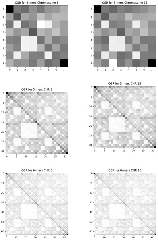
Figure 2.
The frequency Chaos Game Representation for the complete sequence. We present the results for randomly chosen chromosomes 8 and 15. The columns on the left are the results from chromosome 8, and those on the right are from chromosome 15. Each row corresponds to a pixelation level. Top: , middle: , and bottom: .
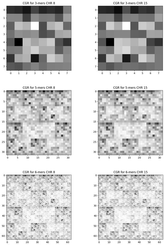
Figure 3.
The frequency Chaos Game Representation for the exon sequence. We present the results for randomly chosen chromosomes 8 and 15. The columns on the left are the results of chromosome 8, and those on the right are from chromosome 15. Each row corresponds to a level of pixelation. Top: , middle: , and bottom: .
Our FCGR results on all chromosomes, for both data sets, employing various scales, reveal geometric patterns encompassing parallel lines and squares indicating self-similarity characteristics in the base pair sequences.
The empty squares in Figure 2 indicate the underrepresentation of specific patterns in the exon chain. This pattern is the already observed “double-scoop” pattern []. The difference in shape from the usual “double-scoop” pattern is due to our choice of the position of each base A, C, G, and T in the CGR. This result is probably related to the fact that there is a strong under-representation of CG dinucleotides in human sequences due to the hypermutability of cytosine. The hypermutability of cytosine refers to its tendency to undergo spontaneous deamination, converting it into uracil. During replication, uracil pairs with adenine instead of guanine, resulting in a C-G to T-A mutation. This process is one of the main causes of the reduction in the frequency of CG dinucleotides in genomic sequences [].
In the exon sequence of chromosome base pairs, in addition to the under-representation of CG pair, we also observed the under-representation of the TA pair. This property manifests through two empty squares in the FCGR representation in Figure 3. To confirm this result, we performed FCGR to k = 2, for chromosomes. In almost all of them, we found that the CG and TA pairs occur less frequently than the other pairs. Visually speaking, this behavior is not as straightforward as in the complete sequence, but it is possible to identify.
Our analysis of chromosome similarity, conducted through Equation (2), revealed fundamental information about genomic organization and composition at different resolution levels. The similarity d between the two data sets is shown in Figure 4 and Table S2. Each column corresponds to the similarity between the chromosome of the entire sequence set and the same chromosome of the exon sequences, calculated on one of the scales . By calculating the distance between these two data sets at different scales, we can discern how the distribution of k-mers varies across each. Our results show that the absence of nonexon regions does not significantly alter the distribution of k-mers in sequences. The chromosome that presents the most significant variation in k is the Y chromosome.
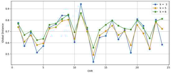
Figure 4.
The similarity between chromosomes composed of entire sequences and chromosomes composed only of exons. The numerical values are in Table S2 (See Supplementary Files).
The Y chromosome is known to have a unique and distinctive genomic composition, as it is highly specialized for functions related to the male sex determinant. Therefore, variations in the patterns of global distance d between the complete sequence of the Y chromosome and the sequence composed only of exons may reflect differences in the organization and function of the intronic and exonic regions of the Y chromosome.
A possible interpretation is that the complete Y chromosome sequences may have distinct d similarity patterns compared with the exonic regions, indicating differences in the organization of the repeating structure and the complexity of the sequences. These differences may be related to the specific function of the Y chromosome in sex determination and reproductive biology.
3.2. Time Series Analysis
We construct the time series from the sequences of base pairs utilizing the mapping rule f established in Section 2. The main statistical characteristics for the two sets of chromosomes are shown in Figure 5, and the numeric values are in Table S1. The time series representation for the set of complete base pair sequences is shown in Figure 6, and the exon sequences can be seen in Figure 7. The different mapping rule could influence the parameter values since we generate a different series for each mapping rule. However, the general behavior of the sequence is preserved, given that the sequence generating process is the same (the DNA sequence).
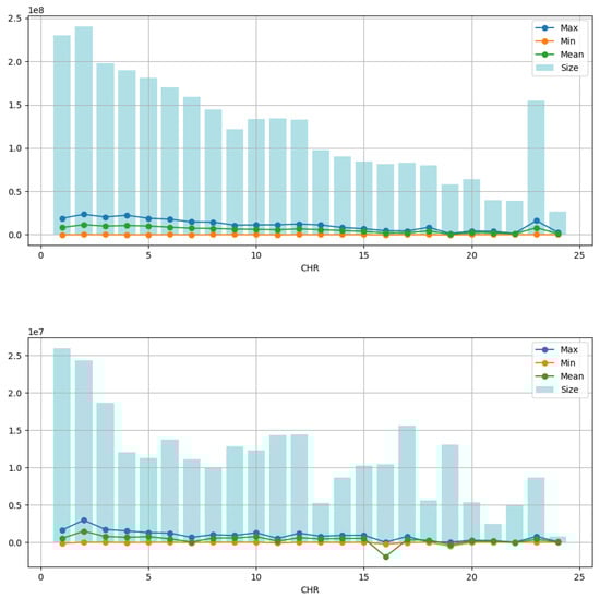
Figure 5.
Time series measurements are represented by mapping the four nitrogenous bases (A, C, G, T) into four discrete values (). The column of bars shows the number of points (size) in each time series. Line charts display the maximum (max), minimum (min), and mean (mean) values of the time series. It is observed that the maximum, minimum, and average values are significantly smaller compared with the total number of points. At the top, we have the measurements for the complete sequence; at the bottom figure, we have the measurements for the exons. The X and Y chromosomes occupy positions 23 and 24 on the “CHR” axis. The numerical values are in Table S1 (See Supplementary Files).
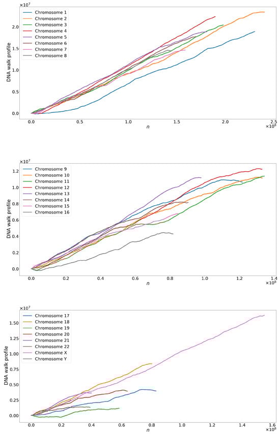
Figure 6.
Time series from the entire sequence of base pairs for human chromosomes.
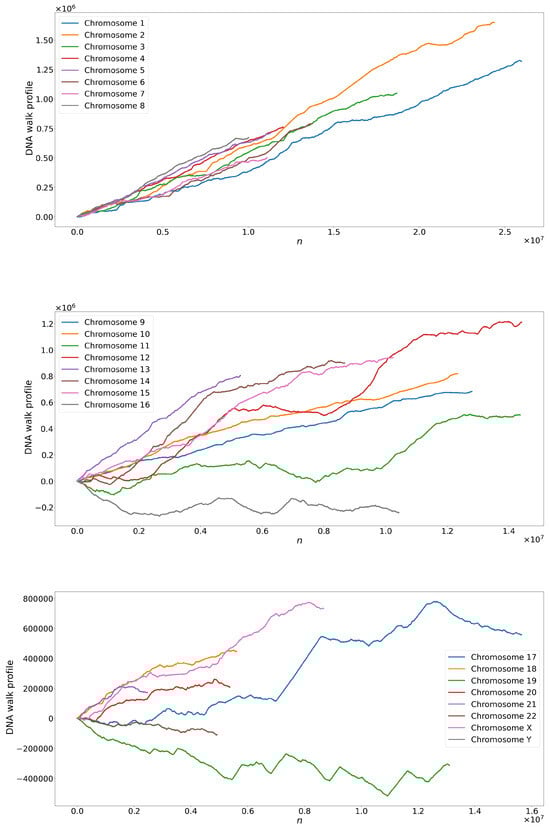
Figure 7.
Time series derived from the coding region of human DNA (exons).
When examining the time series, we observed a notable limitation in the range of maximum, minimum, and average values concerning the total number of points; see Figure 4. This restriction suggests that the variation between the mapped nitrogen base values may be contained within a relatively narrow range, decreasing the limited range in the data. Additionally, we identify repetitive or regular patterns in maximum, minimum, and average values over time by analyzing time series graphs. These patterns suggest the presence of recurring behaviors or cycles in the data, which can be attributed to the intrinsic nature of the underlying process that generates the time series. Combining these characteristics of limited amplitude and repetitive patterns in time series highlights the importance of detailed analysis to understand the structure and dynamics of data using tools such as the complexity–entropy plane and MF-DFA.
3.3. Complexity Entropy
For each one of the 48 chromosomes, we additionally computed the statistical complexity (C) and entropy (E). We employ the Python library ordpy, which was presented and extensively examined in ref. []. This is a useful tool for finding whether the time series is chaotic or stochastic and how these measurements behave at different scales in DNA sequences.
First, we compute the statistical complexity and entropy for scaling segments and . For exons, we obtain and , and for the complete sequences, and . The entropy–complexity plane for this condition is shown in Figure 8. Note that there is a very sharp separation between the two sets. Both sets have high entropy and low statistical complexity, indicating that the time series generated from these base pair sequences are stochastic. This means that the time series exhibits variations and fluctuations that appear random and the evolution of the data over time cannot be described by an exact deterministic relationship. The future course of the series is uncertain and can only be described in terms of probability distributions.
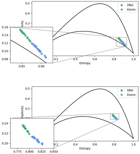
Figure 8.
Complexity–entropy causality plane for complete and exons sequences. At the top, we use , and at the bottom, . The upper (bottom) dashed line represents the maximum (minimum) complexity value as an entropy function.
As defined, based on Shannon entropy, E is associated with the uncertainty of ordinal patterns. The above values for E indicate a great uncertainty related to the distribution of ordinal patterns. The meaning of this is associated with the fact that, although some ordinal patterns are more likely to occur than others, one of them has no predominance of occurrence. In addition, we observed that introns’ presence in DNA sequences makes the complete sequence more complex than sequences composed only of introns (See Figure 8).
We carry out the same procedure for the dimension and . The complexity–entropy plane under this condition is seen in Figure 8. Again, the sequence containing introns has a statistical complexity of and an entropy of , as well as the exon sequences and . At this scale, we observe that there is still a separation for each data set. The set containing introns continues to exhibit greater statistical complexity and lower entropy. However, we observed that the increase in dimension caused a decrease in the uncertainty E and an increase in the statistical complexity C. From this scale, missing patterns appear due to our choice of mapping, which fails to distinguish between some patterns.
A significant connection can be established between complexity–entropy analysis and the Chaos Game Representation (CGR) method, as they reveal complementary insights into the structure and organization of genomic sequences. The visual patterns identified by CGR, which vary in terms of structure and organization, demonstrate an inverse relationship with the entropy and statistical complexity of the sequences. In particular, we observed that more structured and organized patterns (complete sequence), visually evidenced by the CGR, tend to exhibit lower entropy and greater complexity. In comparison, less structured patterns are associated with greater entropy. This relationship suggests that the organization of patterns in the CGR can directly influence the complexity and entropy of genomic sequences, providing a valuable perspective on the multifaceted nature of genome structure.
In other words, at different scales, introns increase the complexity of the sequences while decreasing the uncertainty associated with the occurrence of ordinal patterns.
3.4. MF-DFA
Considering the biological relevance of exons in the production of amino acids and the available computational capacity, we decided to apply the MF-DFA method only to the coding sequences.
The Hurst exponent H measures the degree of correlation in a time series. In random sequences, H is approximately , indicating a weak correlation between nucleotides. The generalized Hurst exponents for some chromosomes are represented in Figure 9. For these sequences, we observed values ranging from to for H, suggesting a persistent behavior across base pairs. This persistence is evidenced by the consistent presence of Adenine and Guanine (or Cytosine and Thymine), where these nitrogenous bases tend to recur within the DNA chain. Moreover, this persistent pattern persists even in the absence of these bases, indicating a sustained trend over time.
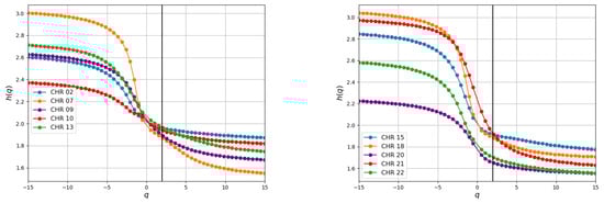
Figure 9.
For coding human chromosomes selected at random, the generalized Hurst exponents are displayed. Comparable behaviors are noted in the remaining chromosomes. The values are made easier to see by the vertical line at .
The spectra for chromosomes exhibit relatively minor variations with q compared with other chromosomes, as illustrated in the column in Table 1. This observation suggests a straightforward fractal structure featuring long-range power-law correlations among nucleotides, which can be adequately described by a limited number of scaling factors. In contrast, the spectra for chromosomes display more pronounced variations with q, indicative of a more heterogeneous sequence characterized by a well-defined multifractal structure. This structure entails long-range power-law correlations among nucleotides and requires a relatively higher number of scaling factors for its description.

Table 1.
Fractal metrics: The first column denotes the chromosome, while the second column displays the Hurst exponent H. The subsequent columns, third through fifth, represent the variations of , , and the symmetry parameter B, respectively.
As can be seen in Figure 10, the multifractal spectra derived from Equation (15) show concave behavior with maximum values at the scaling indices . The degree of multifractality is measured by the width of ; a wider width denotes more heterogeneity in the fractal, suggesting more complexity in the process of generating the investigated series and more difficulty in making predictions, and vice versa. Chromosomes exhibit the highest variation in compared with other chromosomes, while display the lowest, as indicated in the table.
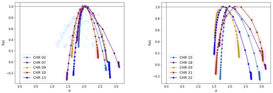
Figure 10.
The spectrum for human chromosomes. Similar responses are noted for the remaining chromosomes.
These results show that the MF-DFA method can distinguish variations in the genetic composition of chromosomes and indicate functional differences between them. A deeper study is necessary to identify which biological characteristic is captured by this method.
The value of the parameter B is more significant than 1 for all chromosomes (except the Y chromosome). Asymmetry in the multifractal spectrum suggests that subsets exhibiting minor fluctuations contribute substantially to the spectrum of DNA sequences.
The difference between the values of the fractal parameters for each chromosome, as shown in Table 1, indicates variation in the complexity of DNA sequences throughout the genome. Each chromosome has a unique set of genes and regulatory regions, and these variations in genomic composition can lead to different fractal patterns. Differences in the values of the fractal parameters can be related to several characteristics, such as the presence of specific genes, sequence repetitions, and regulatory elements.
We want to discuss the results found in some articles, such as [,], where a long-range correlation behavior was observed between base pairs and the nature of persistence in rich and poor sequences in introns, corroborating the results obtained in this article. However, unlike our findings, these studies also indicated a monofractal nature in the sequences used, characterized by a single Hurst exponent. These results differ from those obtained in our work due to the database used. The (multi)fractal analyses in these studies employed fragments of human DNA, such as the HUMHBB sequence and the ECO110K sequence, which are probably the most famous examples of intron-rich and intron-poor sequences, respectively. However, considering the human genome as a whole, it is essential to note that these sequences are relatively small in terms of base pairs.
Our approach, on the other hand, involved using the complete human DNA sequence, aiming for a more comprehensive and representative analysis of fractal properties. This decision was motivated by our intention to explore the full complexity of the human genome, which allowed us to investigate a wider variety of fractal patterns and trends present in DNA sequences. We recognize that choosing smaller sequences may be computationally and methodologically convenient. However, the inclusion of the complete sequence provided a more complete and robust perspective for our analysis, revealing a multifractal nature previously unobserved in the cited works.
4. Conclusions
Our study leveraged the robustness of Chaos Game Representation, ordinal patterns, and the CEP to delve into the influence of intron sequences on human DNA. These methods allowed us to explore structural properties at various scales, providing a comprehensive understanding of the topic. The CGR offers a detailed visual representation of the distribution patterns of nitrogenous bases, indicating that chromosome sequences present better-defined structural patterns. The complexity–entropy plane provides a quantitative analysis of the statistical complexity and entropy of sequences, suggesting that complete sequences have less disorder (entropy) and a more complex structure (greater statistical complexity). On the other hand, MF-DFA revealed multifractal characteristics of the sequences, revealing complex fluctuation patterns at different scales. By using these methods, the following has been shown.
Through the CGR approach, we identified that both sets of chromosomes present geometric figures at different scales, manifested by parallel lines and squares (self-similarity). Furthermore, we detected the underrepresentation of the CG pair in the exons and the underrepresentation of the CG and TA pairs in the complete sequences.
Through MF-DFA analysis of time series generated from DNA sequences, we observed that all chromosomes exhibit a persistent nature, evidenced by in all time series. Furthermore, we identified variations in fractal structure between chromosomes. In particular, chromosomes 05, 07, 12, and 14 demonstrate a more defined fractal structure and greater complexity in the process that generates their time series compared with the others. On the other hand, chromosomes 10, 16, 19, and Y exhibit a less defined fractal structure. Through the symmetry parameter B, we observe that small fluctuations contribute more significantly to the construction of the multifractal spectrum of chromosomes. This variation in fractal parameters highlights the complexity of the dynamic characteristics present in these genomic sequences.
Using the complexity–entropy plane, we find that both of the time series that are generated from chromosomal sequences have low statistical complexity and high entropy, which suggests that they are stochastic. The two data sets are notably situated in distinct locations on the complexity–entropy plane, revealing variations that remain at different scales.
Our findings indicate that the presence of introns in base pair sequences significantly alters the statistical complexity and entropy of the time series. This observation, which holds true across different CEP scales, underscores the importance of considering introns in the analysis of genomic sequences, as they introduce a unique layer of complexity.
While exon regions have traditionally been considered the main areas of interest due to their role in protein coding, nonexonic regions play a variety of critical functions in controlling gene expression, epigenetic regulation, and the formation of three-dimensional structures of DNA. For example, introns, despite not encoding proteins, have been increasingly recognized as important regulators of gene expression and as sites of alternative RNA processing. Furthermore, intergenic and noncoding regions are essential in regulating transcription, modulating chromosomal structure, and genome evolution. Therefore, a possible extension of this work is investigating the fractal properties and complexity in these regions for a comprehensive understanding of the structure and function of the genome, as well as to advance knowledge in molecular biology and genomics.
Supplementary Materials
The following supporting information can be downloaded at https://www.mdpi.com/article/10.3390/fractalfract8060312/s1, Table S1: Statistical characteristics of the time series generated by the sequences of human chromosomes. The first column indicates the chromosome. The column with index N is the size of each sample. The index Max and Min are the maximum and minimum values of the time series generated from each chromosome, and is the mean of the samples. Table S2: The similarity between chromosomes composed of entire sequences and chromosomes composed only of exons. The first column indicates the chromosome, and the others show the scales on which we calculated the similarity.
Funding
J.P. Correia is supported by Coordenação de Aperfeiçoamento de Pessoal de Nível Superior (CAPES). R. Silva acknowledges financial support from CNPq, Brazil (Grant No. 307620/2019-0). M.S.V. thanks CNPq, Brazil (through Grant No. 313207/2021-6) for financial support. D.H.A.L.A. acknowledges and thanks CNPq, Brazil for financial support (through Grant No. 317464/2021-3). L.R.S. thanks CNPq, Brazil (Grant 302057/2017-0) for financial support. This work was developed thanks to the High-Performance Computing Center at the Universidade Federal do Rio Grande do Norte (NPAD/UFRN).
Conflicts of Interest
The authors declare no conflicts of interest.
References
- Savolainen, V.; Cowan, R.S.; Vogler, A.P.; Roderick, G.K.; Lane, R. Towards writing the encyclopaedia of life: An introduction to DNA barcoding. Philos. Trans. R. Soc. B Biol. Sci. 2005, 360, 1805–1811. [Google Scholar] [CrossRef] [PubMed]
- Friedberg, E.C. DNA damage and repair. Nature 2003, 421, 436–440. [Google Scholar] [CrossRef]
- Snustad, D.P.; Simmons, M.J. Principles of Genetics; John Wiley & Sons: Hoboken, NJ, USA, 2015. [Google Scholar]
- Nurk, S.; Koren, S.; Rhie, A.; Rautiainen, M.; Bzikadze, A.V.; Mikheenko, A.; Vollger, M.R.; Altemose, N.; Uralsky, L.; Gershman, A.; et al. The complete sequence of a human genome. Science 2022, 376, 44–53. [Google Scholar] [CrossRef] [PubMed]
- Pareek, C.S.; Smoczynski, R.; Tretyn, A. Sequencing technologies and genome sequencing. J. Appl. Genet. 2011, 52, 413–435. [Google Scholar] [CrossRef] [PubMed]
- Voss, R.F. Evolution of long-range fractal correlations and 1/f noise in DNA base sequences. Phys. Rev. Lett. 1992, 68, 3805. [Google Scholar] [CrossRef] [PubMed]
- Buldyrev, S.V.; Goldberger, A.L.; Havlin, S.; Peng, C.K.; Simons, M.; Stanley, H.E. Generalized Lévy-walk model for DNA nucleotide sequences. Phys. Rev. E 1993, 47, 4514. [Google Scholar] [CrossRef] [PubMed]
- Yu, Z.G.; Wang, B. A time series model of CDS sequences in complete genome. Chaos Solitons Fractals 2001, 12, 519–526. [Google Scholar] [CrossRef]
- Arneodo, A.; Bacry, E.; Graves, P.; Muzy, J.F. Characterizing long-range correlations in DNA sequences from wavelet analysis. Phys. Rev. Lett. 1995, 74, 3293. [Google Scholar] [CrossRef]
- Correia, J.; Silva, R.; Anselmo, D.; da Silva, J. Bayesian inference of length distributions of human DNA. Chaos Solitons Fractals 2022, 160, 112244. [Google Scholar] [CrossRef]
- Costa, M.; Silva, R.; Anselmo, D.; Silva, J. Analysis of human DNA through power-law statistics. Phys. Rev. E 2019, 99, 022112. [Google Scholar] [CrossRef]
- Mandelbrot, B.B. On the geometry of homogeneous turbulence, with stress on the fractal dimension of the iso-surfaces of scalars. J. Fluid Mech. 1975, 72, 401–416. [Google Scholar] [CrossRef]
- Ghil, M.; Benzi, R.; Parisi, G. (Eds.) Turbulence and Predictability in Geophysical Fluid Dynamics and Climate Dynamics; North-Holland Publ. Co.: Amsterdam, The Netherlands; New York, NY, USA, 1985; p. 449. [Google Scholar]
- Mandelbrot, B. Multifractals and 1/ƒ Noise: Wild Self-Affinity in Physics (1963–1976); Springer: New York, NY, USA, 1999. [Google Scholar]
- Olsen, L. A Multifractal Formalism. Adv. Math. 1995, 116, 82–196. [Google Scholar] [CrossRef]
- Achour, R.; Li, Z.; Selmi, B.; Wang, T. A multifractal formalism for new general fractal measures. Chaos Solitons Fractals 2024, 181, 114655. [Google Scholar] [CrossRef]
- Hattab, J.; Selmi, B.; Verma, S. Mixed multifractal spectra of homogeneous moran measures. Fractals 2024, 32, 2440003. [Google Scholar] [CrossRef]
- Selmi, B. A Review on Multifractal Analysis of Hewitt–Stromberg Measures. J. Geom. Anal. 2022, 32, 1–44. [Google Scholar] [CrossRef]
- Georgii, H.O. Gibbs Measures and Phase Transitions; De Gruyter: Berlin, Germany; New York, NY, USA, 2011. [Google Scholar] [CrossRef]
- Fathi, B.N. Analyse multifractale de mesures. C. R. Acad. Sci. Paris Sér. I Math. 1994, 319, 807–810. [Google Scholar]
- Ben Nasr, F.; Bhouri, I.; Heurteaux, Y. The Validity of the Multifractal Formalism: Results and Examples. Adv. Math. 2002, 165, 264–284. [Google Scholar] [CrossRef]
- Jeffrey, H.J. Chaos game representation of gene structure. Nucleic Acids Res. 1990, 18, 2163–2170. [Google Scholar] [CrossRef] [PubMed]
- Cigan, B. Chaos Game Representation of a Genetic Sequence. Available online: https://towardsdatascience.com/chaos-game-representation-of-a-genetic-sequence-4681f1a67e14 (accessed on 25 February 2023).
- Basu, S.; Pan, A.; Dutta, C.; Das, J. Chaos game representation of proteins. J. Mol. Graph. Model. 1997, 15, 279–289. [Google Scholar] [CrossRef]
- Rosso, O.A.; Larrondo, H.; Martin, M.T.; Plastino, A.; Fuentes, M.A. Distinguishing noise from chaos. Phys. Rev. Lett. 2007, 99, 154102. [Google Scholar] [CrossRef]
- Machado, J.T.; Costa, A.C.; Quelhas, M.D. Shannon, Rényi and Tsallis entropy analysis of DNA using phase plane. Nonlinear Anal. Real World Appl. 2011, 12, 3135–3144. [Google Scholar] [CrossRef]
- Zunino, L.; Zanin, M.; Tabak, B.M.; Pérez, D.G.; Rosso, O.A. Complexity-entropy causality plane: A useful approach to quantify the stock market inefficiency. Phys. A Stat. Mech. Its Appl. 2010, 389, 1891–1901. [Google Scholar] [CrossRef]
- Ribeiro, H.V.; Zunino, L.; Mendes, R.S.; Lenzi, E.K. Complexity–entropy causality plane: A useful approach for distinguishing songs. Phys. A Stat. Mech. Its Appl. 2012, 391, 2421–2428. [Google Scholar] [CrossRef]
- Ribeiro, H.V.; Zunino, L.; Lenzi, E.K.; Santoro, P.A.; Mendes, R.S. Complexity-entropy causality plane as a complexity measure for two-dimensional patterns. PLoS ONE 2012, 7, e40689. [Google Scholar] [CrossRef]
- Kantelhardt, J.W.; Zschiegner, S.A.; Koscielny-Bunde, E.; Havlin, S.; Bunde, A.; Stanley, H.E. Multifractal detrended fluctuation analysis of nonstationary time series. Phys. A Stat. Mech. Its Appl. 2002, 316, 87–114. [Google Scholar] [CrossRef]
- Mandelbrot, B.B.; Ness, J.W.V. Fractional Brownian Motions, Fractional Noises and Applications. SIAM Rev. 1968, 10, 422–437. [Google Scholar] [CrossRef]
- Mandelbrot, B.B.; Mandelbrot, B.B. The Fractal Geometry of Nature; WH freeman: New York, NY, USA, 1982; Volume 1. [Google Scholar]
- Wang, W.; Liu, K.; Qin, Z. Multifractal analysis on the return series of stock markets using MF-DFA method. In International Conference on Informatics and Semiotics in Organisations; Springer: Berlin/Heidelberg, Germany, 2014; pp. 107–115. [Google Scholar]
- Rego, C.; Frota, H.; Gusmão, M. Multifractality of Brazilian rivers. J. Hydrol. 2013, 495, 208–215. [Google Scholar] [CrossRef]
- Jader da Silva, J.; Stpŏsíc, B.; Stŏíc, T. Multifractality and complexity of the brazilian agribusiness commodities. Braz. J. Biom. 2016, 34, 258–278. [Google Scholar]
- de Benicio, R.B.; Stošić, T.; De Figueirêdo, P.; Stošić, B.D. Multifractal behavior of wild-land and forest fire time series in Brazil. Phys. A Stat. Mech. Its Appl. 2013, 392, 6367–6374. [Google Scholar] [CrossRef]
- Klug, W.S.; Cummings, M.R.; Spencer, C. Concepts of Genetics, 7th ed.; Pearson Education, Inc.: London, UK, 2003. [Google Scholar]
- Gilbert, W. The exon theory of genes. In Cold Spring Harbor Symposia on Quantitative Biology; Cold Spring Harbor Laboratory Press: Cambridge, MA, USA, 1987. [Google Scholar]
- Rogozin, I.B.; Carmel, L.; Csuros, M.; Koonin, E.V. Origin and evolution of spliceosomal introns. Biol. Direct 2012, 7, 1–28. [Google Scholar] [CrossRef]
- Carroll, S.B.; Doebley, J.; Griffiths, A.J.; Wessler, S.R. Introduction to Genetic Analysis; Springer: Berlin/Heidelberg, Germany, 2015. [Google Scholar]
- Alberts, B. Molecular Biology of the Cell; Garland Science: New York, NY, USA, 2017. [Google Scholar]
- Chow, L.T.; Gelinas, R.E.; Broker, T.R.; Roberts, R.J. An amazing sequence arrangement at the 5 ends of adenovirus 2 messenger RNA. Cell 1977, 12, 1–8. [Google Scholar] [CrossRef] [PubMed]
- De Conti, L.; Baralle, M.; Buratti, E. Exon and intron definition in pre–mRNA splicing. Wiley Interdiscip. Rev. RNA 2013, 4, 49–60. [Google Scholar] [CrossRef]
- National Library of Medicine. Available online: https://www.ncbi.nlm.nih.gov/ (accessed on 23 February 2023).
- Almeida, J.S.; Carrico, J.A.; Maretzek, A.; Noble, P.A.; Fletcher, M. Analysis of genomic sequences by Chaos Game Representation. Bioinformatics 2001, 17, 429–437. [Google Scholar] [CrossRef] [PubMed]
- Deschavanne, P.J.; Giron, A.; Vilain, J.; Fagot, G.; Fertil, B. Genomic signature: Characterization and classification of species assessed by chaos game representation of sequences. Mol. Biol. Evol. 1999, 16, 1391–1399. [Google Scholar] [CrossRef] [PubMed]
- Pandit, A.; Dasanna, A.K.; Sinha, S. Multifractal analysis of HIV-1 genomes. Mol. Phylogenet. Evol. 2012, 62, 756–763. [Google Scholar] [CrossRef] [PubMed]
- Löchel, H.F.; Heider, D. Chaos game representation and its applications in bioinformatics. Comput. Struct. Biotechnol. J. 2021, 19, 6263–6271. [Google Scholar] [CrossRef] [PubMed]
- Wang, Y.; Hill, K.; Singh, S.; Kari, L. The spectrum of genomic signatures: From dinucleotides to chaos game representation. Gene 2005, 346, 173–185. [Google Scholar] [CrossRef] [PubMed]
- Hao, B.L.; Lee, H.C.; Zhang, S.Y. Fractals related to long DNA sequences and complete genomes. Chaos Solitons Fractals 2000, 11, 825–836. [Google Scholar] [CrossRef]
- Ouadfeul, S.A. Multifractal Analysis of SARS-CoV-2 Coronavirus genomes using the wavelet transform. bioRxiv 2020. [Google Scholar] [CrossRef]
- Bandt, C.; Pompe, B. Permutation entropy: A natural complexity measure for time series. Phys. Rev. Lett. 2002, 88, 174102. [Google Scholar] [CrossRef]
- Leyva, I.; Martínez, J.H.; Masoller, C.; Rosso, O.A.; Zanin, M. 20 years of ordinal patterns: Perspectives and challenges. Europhys. Lett. 2022, 138, 31001. [Google Scholar] [CrossRef]
- Unakafov, A.M.; Keller, K. Conditional entropy of ordinal patterns. Phys. D Nonlinear Phenom. 2014, 269, 94–102. [Google Scholar] [CrossRef]
- Pessa, A.A.; Ribeiro, H.V. ordpy: A Python package for data analysis with permutation entropy and ordinal network methods. Chaos Interdiscip. J. Nonlinear Sci. 2021, 31, 063110. [Google Scholar] [CrossRef]
- Zanin, M.; Olivares, F. Ordinal patterns-based methodologies for distinguishing chaos from noise in discrete time series. Commun. Phys. 2021, 4, 190. [Google Scholar] [CrossRef]
- Lopez-Ruiz, R.; Mancini, H.L.; Calbet, X. A statistical measure of complexity. Phys. Lett. A 1995, 209, 321–326. [Google Scholar] [CrossRef]
- Kantelhardt, J.W. Fractal and multifractal time series. arXiv 2008, arXiv:0804.0747. [Google Scholar]
- Halsey, T.C.; Jensen, M.H.; Kadanoff, L.P.; Procaccia, I.; Shraiman, B.I. Fractal measures and their singularities: The characterization of strange sets. Phys. Rev. A 1986, 33, 1141. [Google Scholar] [CrossRef] [PubMed]
- Kurths, J.; Herzel, H. An attractor in a solar time series. Phys. D Nonlinear Phenom. 1987, 25, 165–172. [Google Scholar] [CrossRef]
- Goldman, N. Nucleotide, dinucleotide and trinucleotide frequencies explain patterns observed in chaos game representations of DNA sequences. Nucleic Acids Res. 1993, 21, 2487–2491. [Google Scholar] [CrossRef]
- Li, M.; Chen, S.S. The tendency to recreate ancestral CG dinucleotides in the human genome. BMC Evol. Biol. 2011, 11, 1–9. [Google Scholar] [CrossRef]
- Rosas, A.; Nogueira, E., Jr.; Fontanari, J.F. Multifractal analysis of DNA walks and trails. Phys. Rev. E 2002, 66, 061906. [Google Scholar] [CrossRef] [PubMed]
Disclaimer/Publisher’s Note: The statements, opinions and data contained in all publications are solely those of the individual author(s) and contributor(s) and not of MDPI and/or the editor(s). MDPI and/or the editor(s) disclaim responsibility for any injury to people or property resulting from any ideas, methods, instructions or products referred to in the content. |
© 2024 by the authors. Licensee MDPI, Basel, Switzerland. This article is an open access article distributed under the terms and conditions of the Creative Commons Attribution (CC BY) license (https://creativecommons.org/licenses/by/4.0/).