Article

Rational Approximations for the Oscillatory Two-Parameter Mittag–Leffler Function

by
Aljowhara H. Honain
1,†,
Khaled M. Furati
1,*,†,
Ibrahim O. Sarumi
1,† and
Abdul Q. M. Khaliq
2,†
1
Department of Mathematics, King Fahd University of Petroleum & Minerals, Dhahran 31261, Saudi Arabia
2
Department of Mathematical Sciences, Middle Tennessee State University, Murfreesboro, TN 37132, USA
*
Author to whom correspondence should be addressed.
These authors contributed equally to this work.
Fractal Fract. 2024, 8(6), 319; https://doi.org/10.3390/fractalfract8060319
Submission received: 13 April 2024 / Revised: 13 May 2024 / Accepted: 17 May 2024 / Published: 27 May 2024
(This article belongs to the Special Issue Mittag-Leffler Function: Generalizations and Applications)

Abstract

:
The two-parameter Mittag–Leffler function E α , β is of fundamental importance in fractional calculus, and it appears frequently in the solutions of fractional differential and integral equations. However, the expense of calculating this function often prompts efforts to devise accurate approximations that are more cost-effective. When α > 1 , the monotonicity property is largely lost, resulting in the emergence of roots and oscillations. As a result, current rational approximants constructed mainly for α ( 0 , 1 ) often fail to capture this oscillatory behavior. In this paper, we develop computationally efficient rational approximants for E α , β ( t ) , t 0 , with α ( 1 , 2 ) . This process involves decomposing the Mittag–Leffler function with real roots into a weighted root-free Mittag–Leffler function and a polynomial. This provides approximants valid over extended intervals. These approximants are then extended to the matrix Mittag–Leffler function, and different implementation strategies are discussed, including using partial fraction decomposition. Numerical experiments are conducted to illustrate the performance of the proposed approximants.

1. Introduction

We are concerned with the approximation of the two-parameter Mittag–Leffler function (MLF) E α , β , defined by
E α , β ( z ) = k = 0 z k Γ ( α k + β ) , Re α > 0 , β C , z C .
This entire function generalizes the MLF of one parameter, E α = E α , 1 , and contains several well-known functions as special cases. In particular, E 1 is the exponential function, and E 2 ( z 2 ) and z E 2 , 2 ( z 2 ) are the cosine and sine functions, respectively, among others. For some surveys on the Mittag–Leffler functions, see, for example, [1,2].
The Mittag–Leffler function E α , β ( z ) arises frequently in the solutions of many physical problems described by differential and/or integral equations of fractional order. In the case α ( 1 , 2 ) , the MLF appears naturally in the solutions of fractional diffusion-wave equations, fractional differential equations for motion, and fractional plasma equations (see [3,4,5,6,7]).
Computing the MLF E α , β is usually challenging (devising and implementing suitable algorithms) and expensive (computation time). Although the series (1) converges for all z C , it is impractical or ineffective to use it computationally for | z | 1 because the series converges very slowly. As a result, various methods have been developed to evaluate the MLF. In [8], an algorithm based on the location of the argument z in the complex plane was developed, where for large | z | values, the asymptotic series as | z | was used; for | z | < 1 , the series definition (1) was used; and for values in intermediate regions, the integral representation was used. In [9], an approach based on numerical inversion of the Laplace transform was proposed. However, these approaches are computationally time-consuming (see [10,11] for some CPU time comparisons).
Various rational approximations have been sought to efficiently and accurately approximate E α , β . Some of them are based solely on the series definition and provide accurate approximations for small argument values (see, for example, [12,13,14]). Others are based on the global Padé approach [15], in which a hybrid of the local series definition and the asymptotic series representation is used. These global approximations lead to approximants that are accurate over a wide range of arguments (see [10,11,16,17,18]).
The existing rational approximants are effective when the MLF is completely monotone, which is the case when α ( 0 , 1 ) and β α . However, when α > 1 , as discussed in [19,20,21], for some α - β combinations, E α , β is often oscillatory with multiple real zeros. In these situations, the rational approximants might fail to trace the oscillation profile and match the large zeros.
In this paper, we consider in the α β -plane the strip
Ω = { ( α , β ) : 1 < α < 2 , β 1 } .
The regions where E α , β is monotone and where it is oscillatory are classified by studying the zeros of its derivative. Additionally, we introduce new rational approximants that sufficiently capture more of the MLF roots and can effectively trace their oscillations. This is achieved by decomposing E α , β with real roots into another weighted Mittag–Leffler function devoid of roots, accompanied by a polynomial. Based on this decomposition, we construct new rational approximants as a sum of the global Padé approximant and a polynomial. Using this approach, we are able to sufficiently capture many roots of E α , β by choosing the appropriate degree of the polynomial. Further, we generalize these approximants to the matrix MLF and discuss different approaches in which the approximant can be implemented for matrix arguments. Apart from the computation cost, all approaches yield close approximations.
Numerical experiments are presented to illustrate the performance of our approximants. Considering the MLF with scalar arguments, we observe the limitations of the existing global Padé approximants in approximating the oscillatory MLFs. It is then demonstrated that the new approximants introduced here are able to improve the situation, thereby providing sufficiently accurate approximations. For the matrix MLF, we consider four approaches for computing the rational approximants and compare them to the matrix MLF algorithm developed in [22]. Using the values obtained from this algorithm as a reference, it is shown that our approximants provide close values with significantly less computation time.
The rest of this paper is organized as follows. A characterization of the oscillatory behavior of the MLF is given in Section 2. In Section 3, the derooting representation is discussed. Global Padé approximants of the MLF with scalar and matrix arguments are discussed in Section 4 and Section 5, respectively. Some applications to the evaluation of solutions of fractional evolution equations are discussed in Section 6.

2. Monotonicity and Oscillatory Properties

In this section, we characterize the oscillatory behavior of
E α , β ( t ) , ( α , β ) Ω , t 0 .
For the discussion that follows, the following formula for the derivative [1] plays a fundamental role:
d d t E α , β ( t ) = 1 α E α , β + α 1 ( t ) ( β 1 ) E α , β + α ( t ) .
Since E α , β ( 0 ) = 1 / Γ ( β ) , it follows from (3) that
d d t E α , β ( 0 ) = 1 α 1 Γ ( β + α 1 ) β 1 Γ ( β + α ) = 1 Γ ( β + α ) < 0 .
The function E α , β ( t ) , t 0 , is known to be completely monotone for 0 < α 1 , β α . However, this monotonicity is not necessarily preserved when ( α , β ) Ω , since either the function or its derivative could have roots. On the other hand, it was established in [20] that E α , β has at most a finite number of roots when ( α , β ) Ω . Thus, E α , β ( t ) is monotone for sufficiently large t. Furthermore, it was shown in [20] that there exists only one zero when α is sufficiently close to 1, while the number of zeros increases as α increases toward 2.
In Figure 1, the curve ϕ is the boundary given in Table 1 in [20] such that E α , β has a finite number of real roots when ( α , β ) is below it and none above it. However, the function in the region below ϕ ( α ) differs with respect to the number of roots. Typically, the number of roots increases as α approaches 2. Similarly, we constructed the boundary ψ for the derivative. The corresponding data are presented in Table 1.
The monotonicity and oscillatory behavior of E α , β are characterized by the different regions marked in Figure 1 and described in Table 2. It follows from (4) that E α , β ( t ) is monotonically decreasing for ( α , β ) in regions (D) and (F). In regions (B) and (C), although the function has no real roots, it could have a finite number of oscillations due to the roots of the derivative.
Remark 1.
Since E α , β ( t ) 0 as t , it is obvious that each root of it is followed by at least one root of its derivative. This is consistent with the inequality
ϕ ( α ) < ψ ( α ) .
For the region below the line β = α + 1 , which includes the regions (A), (B), and (D), the following decomposition is presented in [19],
E α , β ( t ) = g α , β ( t ) + f α , β ( t ) , t > 0 , β < α + 1 ,
where the function f α , β ( t ) is asymptotically approaching zero as t and g α , β ( t ) is an oscillatory function.
When β = 1 and 1 < α < 2 , the function f α , 1 ( t ) is known to be a completely monotonic function, while the function g α , 1 ( t ) is oscillatory with exponentially decreasing amplitude [3]. The properties of E α , 1 < α < 2 , such as monotonicity, roots, and oscillatory behavior, have been discussed in detail in [23].
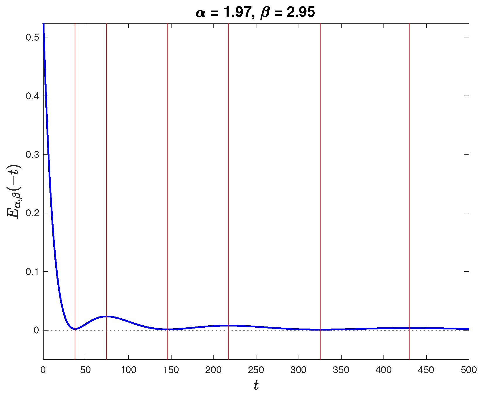
In region (B), although E α , β ( t ) has no roots as it decays to zero, it undergoes oscillations due to the roots of its derivative, as demonstrated in Figure 2. This behavior is also consistent with the oscillatory nature of g α , β there. On the other hand, in region (D), in which E α , β is monotone, the behavior of the oscillatory function g α , β fades away and f α , β ( t ) dominates.

3. Derooting Decomposition

A key step in accurately approximating E α , β ( t ) when 1 < α < 2 is to capture its oscillatory behavior and roots. However, in region (A), in general, the number of roots could exceed those of the rational approximants. This makes these approximants valid only for small arguments.
A derooting approach can be used to extend the validity of the rational approximants to large intervals. For this purpose, we use the following recursive identity [24]
E α , β ( t ) = t r E α , β + α r ( t ) + P α , β r 1 ( t ) , α > 0 , β > 0 , t R , r = 0 , 1 , 2 , ,
where
P α , β r 1 ( t ) : = k = 0 r 1 t k Γ ( α k + β ) , r = 1 , 2 , 3 , 0 , r = 0 .
In this identity, E α , β is decomposed into another MLF with a shifted second parameter and a polynomial of degree r 1 . This allows us to replace the parameters ( α , β ) in region (A) with parameters ( α , β + α r ) above the boundaries ϕ ( α ) or above ψ ( α ) . Consequently, we obtain a function E α , β + α r that has no roots or could even be monotone. Therefore, the approximation of E α , β ( t ) , 1 < α < 2 , with a finite number of real roots can be replaced by approximating another one that has no roots or one that is monotone.

4. Rational Approximation

Based on the global rational approximation technique introduced for transcendental functions in [15], a variety of global Padé approximants for E α , β ( t ) , 0 < α < 1 , have been developed and implemented [10,11,16,17,18]. These approximants are still valid for E α , β ( t ) , 1 < α < 2 , over intervals in which the number of its roots does not exceed the number of approximant roots. This renders these approximants inadequate when approximating the MLF over an interval in which it has multiple roots, as is the case when ( α , β ) is in region (A) in Figure 1.
In general, the global Padé approximation R α , β m , n ( t ) , where m and n are positive integers, for E α , β ( t ) takes the form [10,11]
R α , β m , n ( t ) = 1 Γ ( β α ) p 1 + p 2 t + t ν 1 q 0 + q 1 t + + t ν , v = m + n 1 2 .
The construction of the global Padé approximation depends on the series definition (1) of the MLF as well as its asymptotic expansion, given by the following theorem:
Theorem 1
([25]). Let α ( 0 , 2 ) , β C and μ R , π α 2 < μ < min { π , π α } . Then, for μ   | arg z | π ,
E α , β ( z ) = k = 1 n ( z ) k Γ ( β α k ) + O | z | ( n + 1 ) , a s | z | , n 1 .
It was shown in [10] that the approximant R α , β m , n has the asymptotic error
| E α , β ( t ) R α , β m , n ( t ) | = O t m n 1 2 , m n + 1 ,   as t 0 , O t ( n + 1 ) , n > 1 ,   as t .
In the rest of this section, we consider the global Padé approximants R α , β 7 , 2 and R α , β 13 , 4 , developed in [10,11], and examine their performance when 1 < α < 2 . Then, we describe how the derooting decomposition leads to approximants with an increased number of roots, enabling them to better approximate the roots of the MLF.

4.1. Global Padé Approximation

For { ( α , β ) : 1 < α < 2 , β 1 , α β } , we consider the global Padé approximants
R α , β 7 , 2 ( t ) = 1 Γ ( β α ) p 1 + p 2 t + p 3 t 2 + t 3 q 0 + q 1 t + q 2 t 2 + q 3 t 3 + t 4 , t 0 ,
and
R α , β 13 , 4 ( t ) = 1 Γ ( β α ) p 1 + p 2 t + + p 7 t 6 + t 7 q 0 + q 1 t + q 2 t 2 + + q 7 t 7 + t 8 , t 0 ,
where the coefficients, respectively, satisfy the systems
1 0 0 a 0 0 0 0 0 1 0 a 1 a 0 0 0 0 0 1 a 2 a 1 a 0 0 0 0 0 a 3 a 2 a 1 a 0 0 0 0 a 4 a 3 a 2 a 1 0 0 0 a 5 a 4 a 3 a 2 0 0 1 0 0 0 b 0 p 1 p 2 p 3 q 0 q 1 q 2 q 3 = 0 0 0 1 a 0 a 1 b 1 ,
1 0 0 0 0 0 0 a 0 0 0 0 0 0 0 0 0 1 0 0 0 0 0 a 1 a 0 0 0 0 0 0 0 0 0 1 0 0 0 0 a 2 a 1 a 0 0 0 0 0 0 0 0 0 1 0 0 0 a 3 a 2 a 1 a 0 0 0 0 0 0 0 0 0 1 0 0 a 4 a 3 a 2 a 1 a 0 0 0 0 0 0 0 0 0 1 0 a 5 a 4 a 3 a 2 a 1 a 0 0 0 0 0 0 0 0 0 1 a 6 a 5 a 4 a 3 a 2 a 1 a 0 0 0 0 0 0 0 0 0 a 7 a 6 a 5 a 4 a 3 a 2 a 1 a 0 0 0 0 0 0 0 0 a 8 a 7 a 6 a 5 a 4 a 3 a 2 a 1 0 0 0 0 0 0 0 a 9 a 8 a 7 a 6 a 5 a 4 a 3 a 2 0 0 0 0 0 0 0 a 10 a 9 a 8 a 7 a 6 a 5 a 4 a 3 0 0 0 0 0 0 0 a 11 a 10 a 9 a 8 a 7 a 6 a 5 a 4 0 0 0 0 1 0 0 0 0 0 0 0 b 0 b 1 b 2 0 0 0 0 0 1 0 0 0 0 0 0 0 b 0 b 1 0 0 0 0 0 0 0 0 0 0 0 0 0 0 b 0 p 1 p 2 p 3 p 4 p 5 p 6 p 7 q 0 q 1 q 2 q 3 q 4 q 5 q 6 q 7 = 0 0 0 0 0 0 0 1 a 0 a 1 a 2 a 3 b 3 b 2 b 1 ,
a j = ( 1 ) j + 1 Γ ( β α ) Γ ( β + j α ) , b j = ( 1 ) j + 1 Γ ( β α ) Γ ( β ( j + 1 ) α ) , j = 0 , 1 , .
Remark 2.
As mentioned in [11], it is important to highlight that systems (12) and (13), for determining the coefficients of the approximants R α , β 7 , 2 and R α , β 13 , 4 , exhibit relatively high condition numbers. Consequently, solving these systems necessitates careful attention to avoid accuracy loss due to possible ill-conditioning. In the implementations, we make use of the MATLAB function “linsolve” or the corresponding Python function “scipy.linalg.solve”, which can handle this range of condition numbers.
Computationally, it is observed that R α , β 13 , 4 has at most three real roots, while R α , β 7 , 2 has exactly one real root. Consequently, in approximating some of the oscillatory MLFs, each approximant is only able to trace the function up to its largest root. To illustrate the accuracy and limitations of both approximants when 1 < α < 2 , we compare them with the MATLAB routines ml [9] and ml_matrix [22] for the scalar and matrix arguments, respectively, as our reference values. Other implementations of the MLF, such as the MATLAB function mlf [26] and the Mathematica MittagLefflerE function, can also be used. However, these functions are not available for Matrix arguments, which are of primary interest in the current work. As such, we adopt those in the aforementioned references for our comparisons.
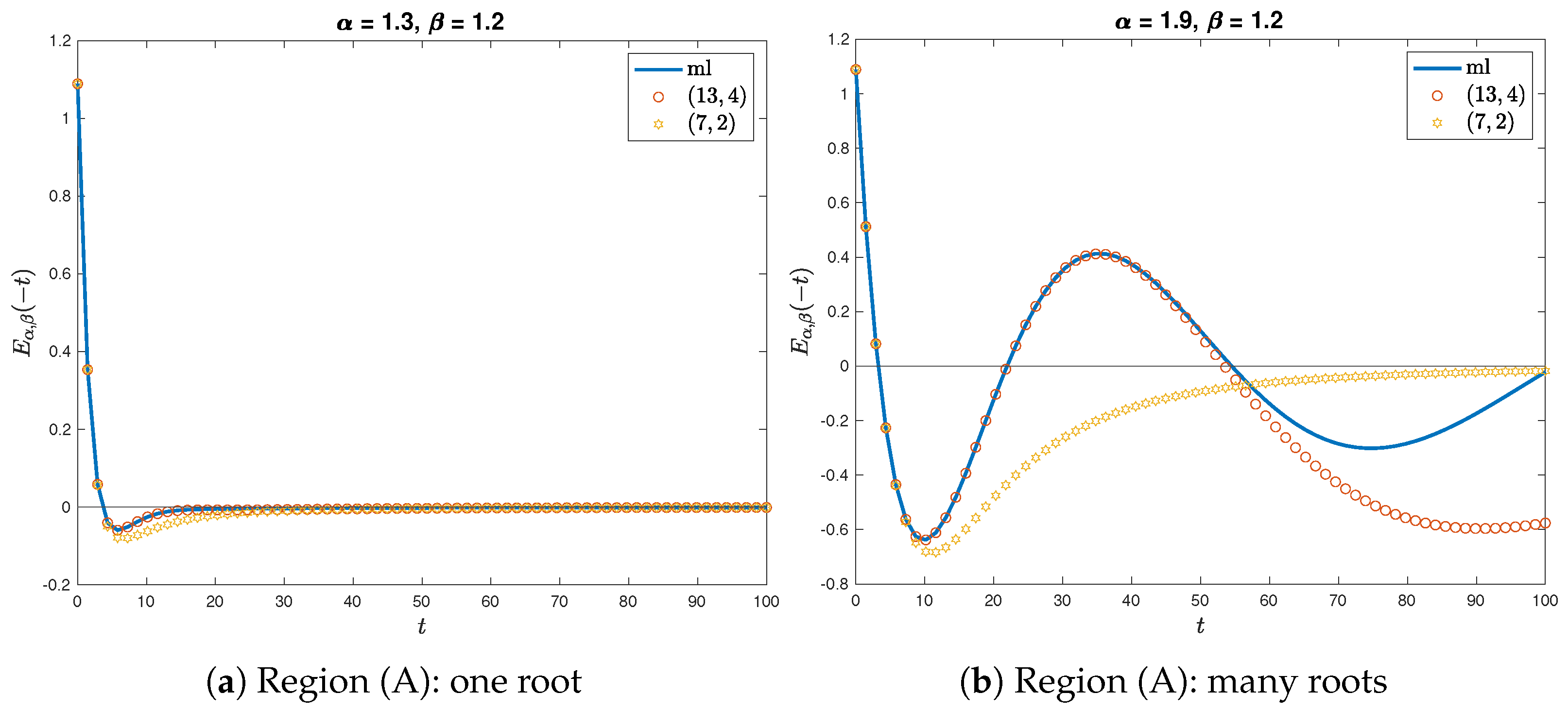
In Figure 3, two examples from region (A) are shown. In plot (a), the MLF has only one root, which is typically the case for 1 < α < 1.4 . As observed, R α , β 13 , 4 provides a good approximation in this case. In plot (b), the MLF has many roots, which is typically the case as α approaches 2. As expected, each approximant fails beyond its largest root to capture the oscillations of the MLF.
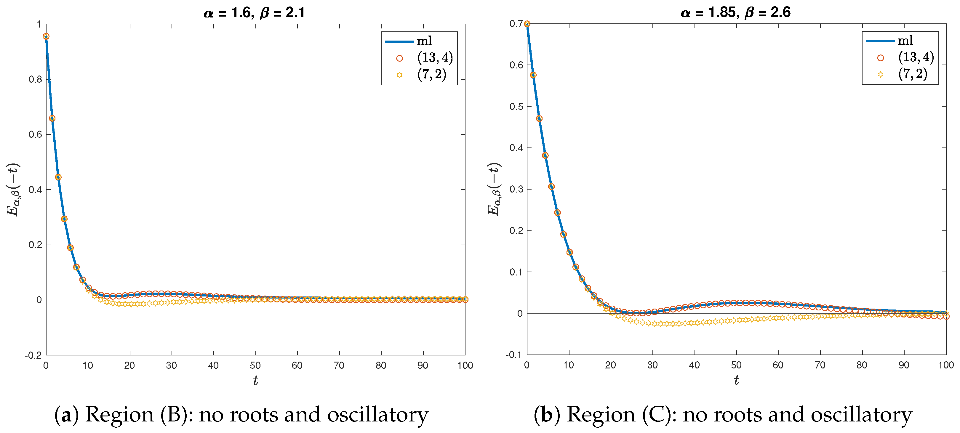
In Figure 4, typical cases from regions (B) and (C) are shown. The corresponding MLFs in both regions are root-free but are oscillatory. As shown, R α , β 13 , 4 is sufficiently accurate for an extended interval. However, eventually, it takes negative values, as shown in plot (b).
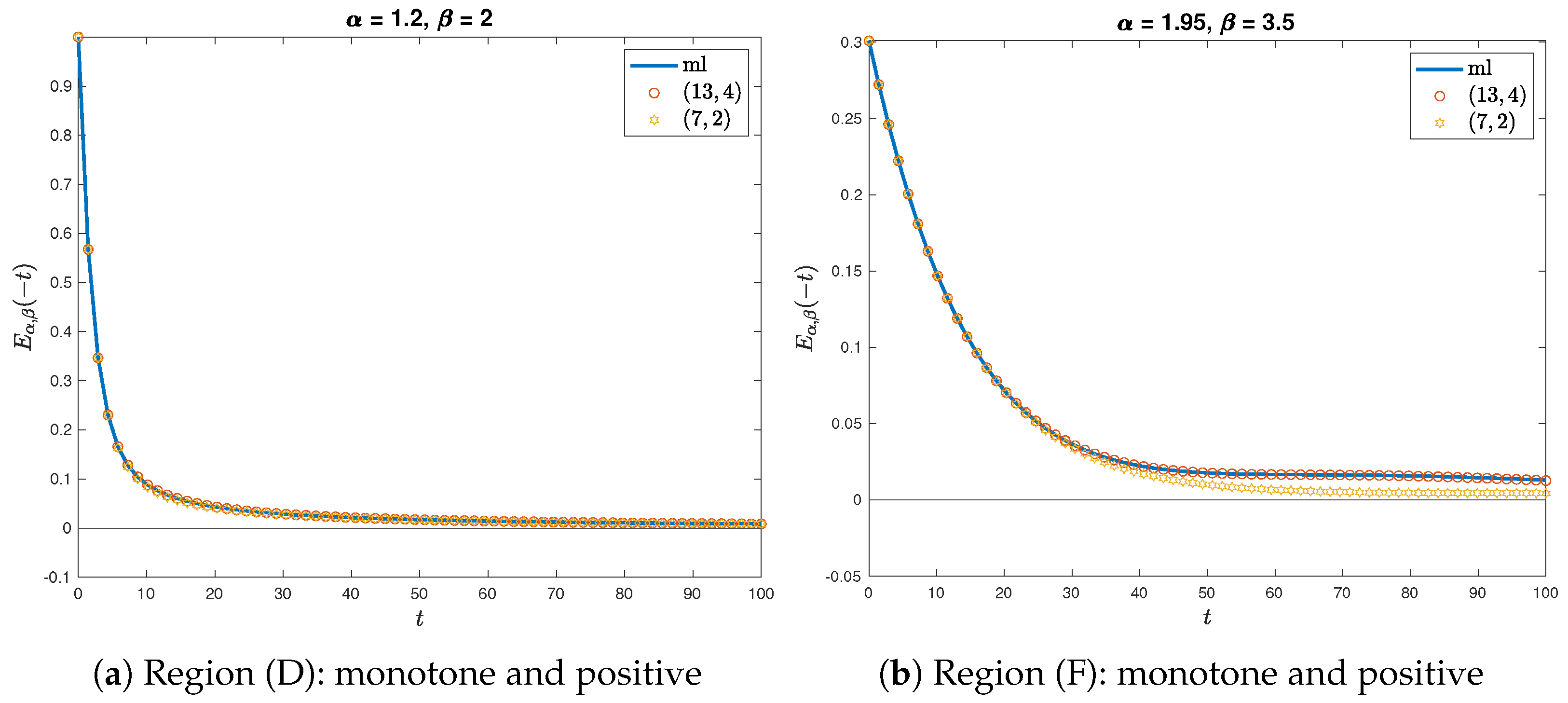
In Figure 5, typical cases from regions (D) and (F) are illustrated. In both regions, the MLF is monotone and globally positive. As can be clearly seen, R α , β 13 , 4 is a good approximation for an extended interval.
As general guidelines, we have the following:
  • When ( α , β ) is in region (A), the existing global Padé approximants are not effective over extended intervals due to the existence of roots.
  • When ( α , β ) is in region (B) or (C), more accurate approximants should be used due to the oscillatory behavior of the MLF.
  • When ( α , β ) is in region (D) or (F), the approximant R α , β 13 , 4 is sufficiently accurate since the MLF is globally monotone.

4.2. Rational Approximation for Oscillatory MLFs

As observed in the above subsection, when ( α , β ) lies below the boundary ψ ( α ) in Figure 1, then more accurate and multi-root approximants are essential for extended intervals. Next, we propose a class of rational approximants that have the desirable performance.
It follows from (6) that we can write
E α , β ( t ) = ( t ) r E α , β + α r ( t ) + P α , β r 1 ( t ) , t > 0 .
Let R α , β m , n be the global Padé approximants described in [10]. We introduce the rational approximant
E α , β ( t ) R α , β m , n , r ( t ) , t > 0 ,
where
R α , β m , n , r ( t ) : = ( t ) r R α , β + α r m , n ( t ) + P α , β r 1 ( t ) , r = 0 , 1 , 2 , .
Note that as a special case, we have
R α , β m , n , 0 = R α , β m , n .
The integer r could be chosen so that ( α , β + α r ) lies above the boundary ψ ( α ) in Figure 1. As demonstrated in the previous subsection, this shifting of parameters would enhance the performance of R α , β + α r m , n since in this case, E α , β + α r ( t ) is root-free and non-oscillatory. Furthermore, r could be chosen large enough so that the approximant R α , β m , n , r captures the desired number of roots and the oscillations of E α , β over an extended interval.

4.3. Asymptotic Behavior of the Approximation Error

We define the error
e α , β m , n , r ( t ) : = E α , β ( t ) R α , β m , n , r ( t ) .
By subtracting the decompositions (14) and (16), and then using the asymptotic error (9), we can determine the asymptotic behavior:
| e α , β m , n , r ( t ) | = | ( t ) r | E α , β + α r ( t ) R α , β + α r m , n ( t ) = t r O t m n 1 2 , m n + 1 ,   as t 0 , O t ( n + 1 ) , n > 1 ,   as t , = O t m n 1 2 + r , m n + 1 ,   as t 0 , O t n 1 + r , n > 1 ,   as t .
Note that although the exponent ( n 1 + r ) in the error term (17) becomes positive as t when r > n + 1 , large values of r increase the number of roots in the modified approximant R α , β m , n , r , which improves its capability to capture the oscillations of the MLF over an extended interval. Consequently, the actual error starts to grow only after the final root of the approximant.
The performance of the generalized approximant R α , β 13 , 4 , r when ( α , β ) is in regions (A) and (C) is demonstrated in Figure 6 and Figure 7, respectively, where
e α , β m , n , r ( t ) : = E α , β ( t ) R α , β m , n , r ( t ) .
As can be observed, the interval of the approximation can be extended by increasing r. The generalized approximant R α , β 7 , 2 , r has the same features, although it is not as accurate as R α , β 14 , 3 , r , as shown in Figure 8.

5. Approximation of the Matrix Mittag–Leffler Function

In this section, we study the approximation of the matrix MLF, defined by [27]
E α , β ( A ) = k = 0 A k Γ ( α k + β ) , Re α > 0 , β C , A C n × n .
Using the definition of rational functions of matrices (see [28]), we define the global Padé approximation of E α , β ( A ) as
R α , β m , n ( A ) : = 1 Γ ( β α ) [ q ( A ) ] 1 p ( A ) ,
for some appropriate matrix A, where p and q denote the numerator and denominator, respectively, of Γ ( β α ) R α , β m , n . Furthermore, by extending the decomposition (6) to matrix arguments, we define the rational approximant
R α , β m , n , r ( A ) = ( A ) r R α , β + r α m , n ( A ) + P α , β r 1 ( A ) , r = 0 , 1 , 2 , ,
where P α , β r 1 is the polynomial given by (7).
Several approaches exist for extending a scalar rational function to matrix arguments. For a comprehensive overview, we recommend consulting [28]. Next, we discuss some approaches for implementing (19) and compare their accuracies and computation times.
1.
Linear system approach
A straightforward approach is to evaluate p ( A ) and q ( A ) using efficient methods for the evaluation of matrix polynomials, such as the Paterson–Stockmeyer method and Horner’s method (nested multiplication) [28]. Additionally, the powers A 2 , A 3 , , can be precomputed and used in the computation of both p ( A ) and q ( A ) to minimize the overall cost. It is noteworthy that research in the field of matrix polynomial evaluation is increasingly active. In particular, a new family of methods for evaluating matrix polynomials, which are more efficient than the established Paterson–Stockmeyer method, was proposed in [29]. This area could be a subject of future research for us, as this section concentrates on introducing general techniques for approximating the MLF matrix using rational approximation, aiming for a general comparison.
Using this approach, the approximant R α , β m , n ( A ) is obtained by solving the matrix system
q ( A ) R α , β m , n ( A ) = p ( A ) .
This requires solving N systems for an N × N matrix.
2.
Partial fraction approach
Partial fraction decomposition is known to provide an efficient form for evaluating rational functions. For the global Padé approximants, it was discussed in [10,11] that these approximants have complex conjugate roots, which can contribute to efficient implementation. As an example, the approximant R α , β 13 , 4 ( t ) , admits the partial fraction decomposition
R α , β 13 , 4 ( t ) = i = 1 4 c i t s i + c ¯ i t s ¯ i ,
where c 1 , c 2 , c 3 , c 4 and s 1 , s 2 , s 3 , s 4 are the non-conjugate residues and poles, respectively. This expression can be simplified as
R α , β 13 , 4 ( t ) = 2 Re i = 1 4 c i t s i .
So, for a matrix argument A, the approximant can be calculated as
E α , β ( A ) R α , β 13 , 4 ( A ) = 2 Re j = 1 4 c j A s j I 1 ,
where I is the identity matrix.
For example, in the implementation using the partial fraction approach, the partial fraction decompositions (22) are used to compute the matrix-vector products as outlined below.
For a given square matrix A and a vector v, the matrix-vector product E α , β ( A ) v is computed using (20) as
E α , β ( A ) v R α , β m , n , r ( A ) v : = ( A ) r R α , β + α r m , n ( A ) v + P α , β r 1 ( A ) v ,
where the term
R α , β + α r m , n ( A ) v ,
is computed using the partial fraction decomposition approach. From (23), we use the approximation
E α , β + α r ( A ) v R α , β + α r m , n ( A ) v = 2 Re j = 1 4 c j A s j I 1 v .
By solving the systems
A s j I x j = v , for j = 1 , 2 , 3 , 4 ,
we obtain
E α , β + α r ( A ) v 2 Re j = 1 4 c j x j ,
where x j , are the solutions of the linear systems (24). As such, no matrix inversion is required. Moreover, using the partial fraction decomposition of the rational approximations is considered an efficient and cost-effective alternative. As mentioned in [11], the poles and residues in the partial fraction decomposition (22) rely on α and β . Therefore, their computation can be achieved independently of the argument A. The Python or MATLAB “residue” function could be used for this purpose.
3.
Matrix diagonalization approach
When the matrix argument A is diagonalizable, a scenario frequently encountered in matrices derived from the semi-discretization of partial differential equations, then the factorization A = Z D Z 1 could be considered, where D is the diagonal matrix containing the eigenvalues, and the columns of Z are the corresponding eigenvectors. In this case, the matrix MLF can be computed as [28,30]
E α , β ( A ) = Z E α , β ( D ) Z 1 = Z diag ( E α , β ( λ i ) ) Z 1 .
Accordingly, the approximant R α , β m , n can be computed as
R α , β m , n ( A ) = Z diag ( R α , β m , n ( λ i ) ) Z 1 .
By employing this approach, we only need to calculate the rational approximation for scalar arguments and perform matrix multiplications, which considerably reduces the computational time. We note that using the diagonalization approach is advisable only under the condition that the matrix is guaranteed to be well conditioned [28].
Remark 3.
The above approaches for computing the MLF matrix are discussed for completeness and general comparisons. However, they are mainly developed to compute the matrix-vector products involved in the implementation of numerical methods for solving fractional differential equations. To the best of our knowledge, computing matrix-vector products involving the MLF remains a fundamental challenge, as current algorithms for evaluating the MLF of scalar or matrix arguments [8,9,22] require considerable implementation cost. Therefore, developing such rational approximants is essential, as they have been proven to offer comparable accuracy and efficient approximations at a low cost.
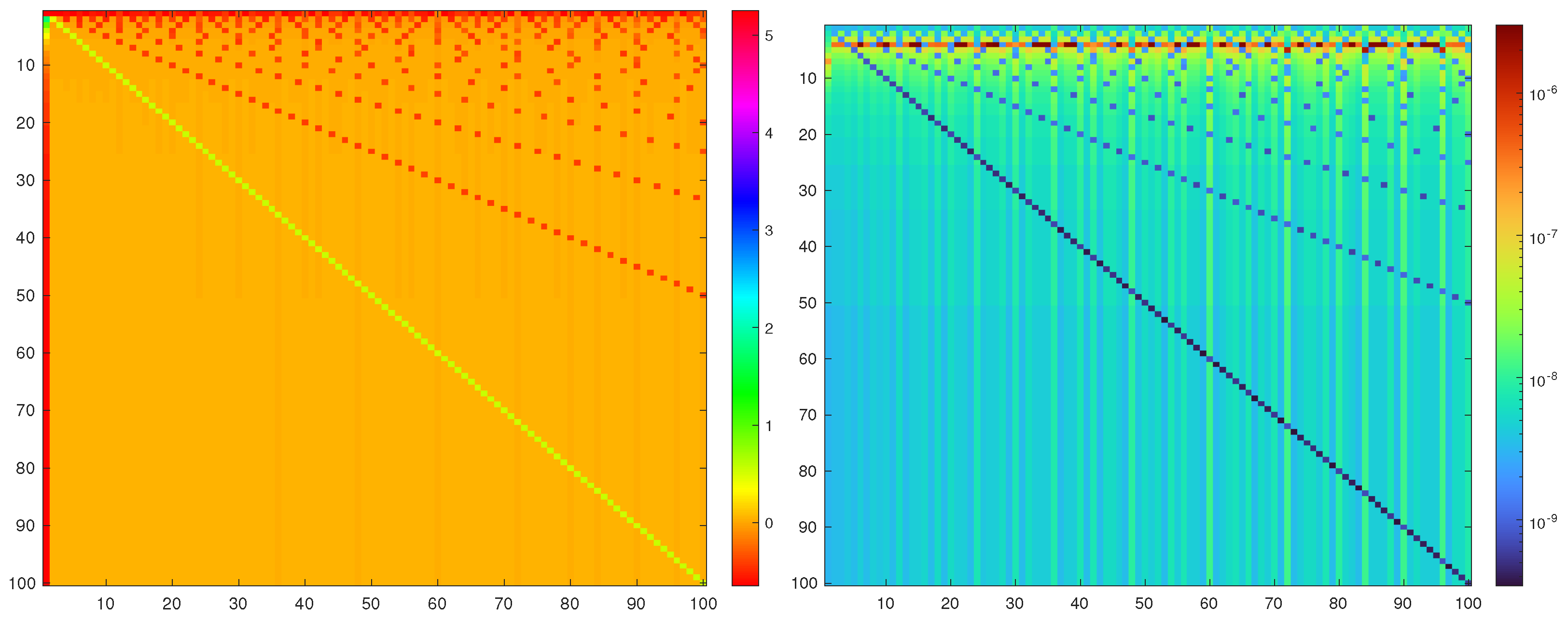
For experimental purposes, we evaluate the performance of the approximant (16) when applied to the Redheffer matrix of size 100 × 100, comparing it with the reference values obtained by the ml_matrix function. In Figure 9, a color map shows the component-wise values and relative errors for R α , β 13 , 4 , with ( α , β ) = ( 1.9 , 1 ) , calculated using partial fractions. Table 3 presents a comparison of the absolute errors, relative errors, and runtimes for the different techniques in computing R α , β 13 , 4 . The absolute and relative errors are given by
E α , β ( t ) R α , β m , n ( t ) ,
and
E α , β ( t ) R α , β m , n ( t ) E α , β ( t ) ,
respectively.

6. Applications and Numerical Experiments

Here, we present some applications of the general Padé approximant (16) related to fractional oscillation equations, where MLFs arise naturally as solutions. Numerical experiments are included to highlight the efficiency and accuracy of these approximants.

6.1. Application: Fractional Plasma Oscillations

The fractional plasma oscillation model, described in [31], is given by
D α c u ( t ) + A u ( t ) = f ( t ) , u ( 0 ) = u 0 , u ( 0 ) = u 1 ,
where D α c denotes the Caputo fractional derivative of order α ( 1 , 2 ) , defined by
D α c u ( t ) : = 1 Γ ( 2 α ) 0 t ( t τ ) 1 α u ( τ ) d τ , 1 < α < 2 , u ( t ) , α = 2 .
The constant A is the fractional electron plasma frequency and f ( t ) is the electric field. We consider the model with a static electric field and with no electric field.

6.1.1. Fractional Plasma Oscillation Model with a Static Electric Field

Consider the special case of problem (25),
D α c u ( t ) + u ( t ) = 1 , u ( 0 ) = 1 , u ( 0 ) = 1 .
The exact solution for this initial value problem is
u ( t ) = E α t α t E α , 2 t α + t α E α , α + 1 t α .
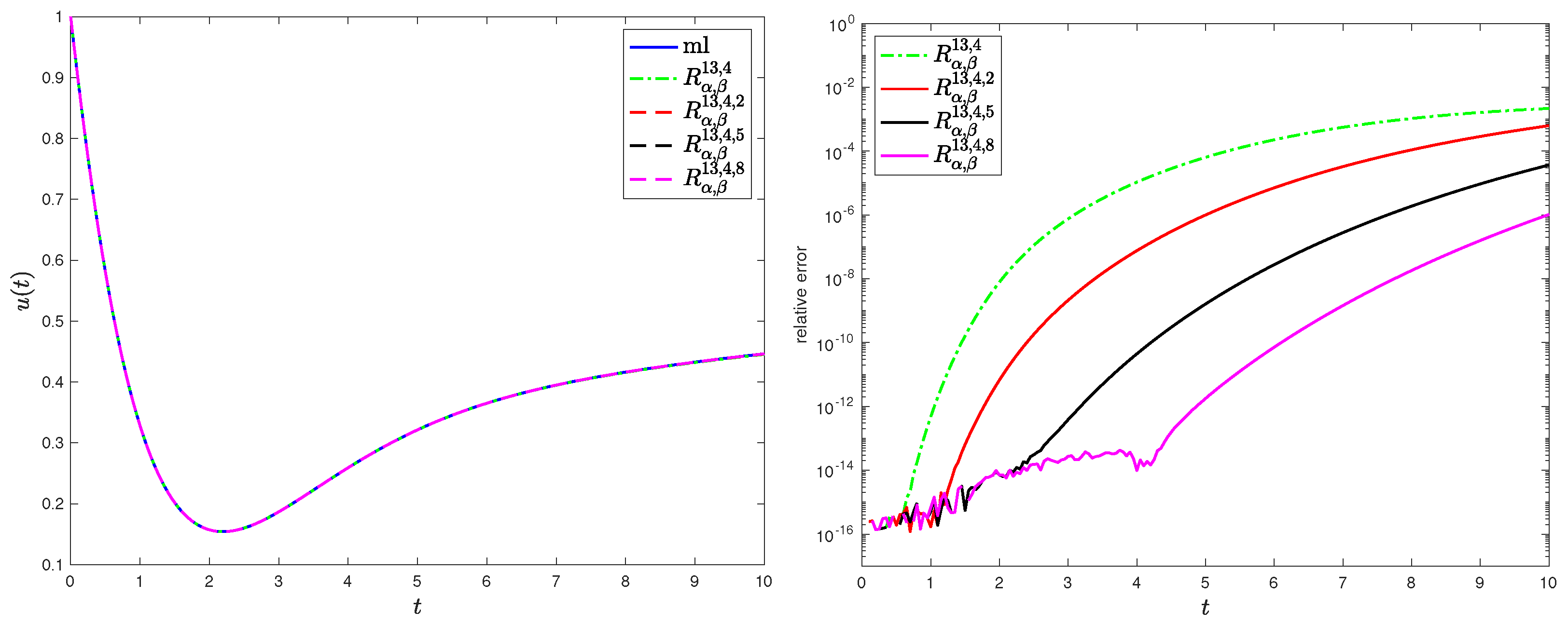
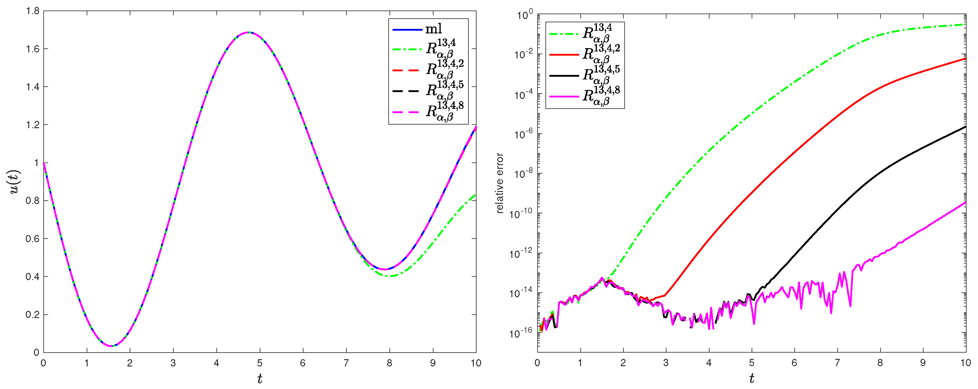
In Figure 10, a comparison of the approximations for (26) when α = 1.2 is provided. Considering the three terms in (26), the pair ( α , β ) with β = 1 falls within region (A) of the phase diagram in Figure 1, where the MLF is oscillatory. Meanwhile, the pairs ( 1.2 , 2 ) and ( 1.2 , 2.2 ) fall within regions (D) and (F), respectively, where the MLF has no real roots and no oscillations. A similar comparison for α = 1.9 is shown in Figure 11. In this case, the terms E 1.9 , 1 and E 1.9 , 2 correspond to ( α , β ) in parts of region (A) where the MLF is highly oscillatory and has many real roots.
To illustrate the computational efficiency, Table 4 shows that R α , β 13 , 4 and R α , β 13 , 4 , r with r = 2 , 5 , 8 exhibit significantly lower computation costs (in terms of time) compared to the ml function. Moreover, while the modified approximant R α , β 13 , 4 , 8 yields more accurate approximations than R α , β 13 , 4 in comparison to the reference values, they have comparable computation times.

6.1.2. Fractional Plasma Oscillation Model with No Electric Field

Consider the initial values problem
D α c u ( t ) + u ( t ) = 0 , u ( 0 ) = 0.2 , u ( 0 ) = 0.1 .
The exact solution of this problem is given by
u ( t ) = 0.2 E α t α + 0.1 t E α , 2 t α .
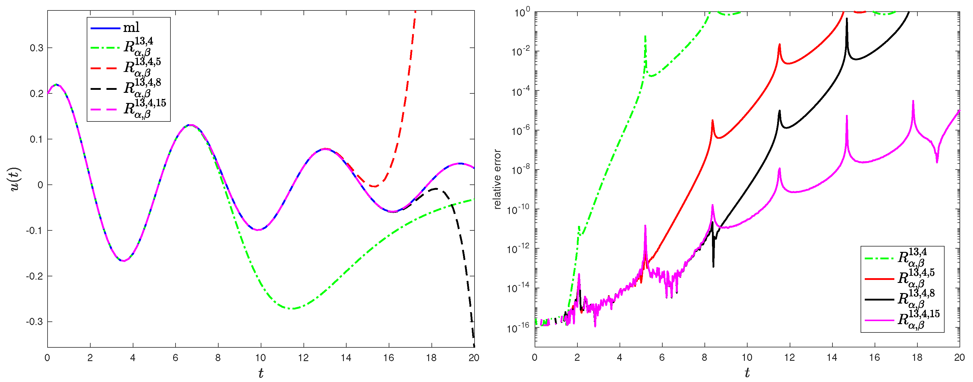
A comparison of the approximations of (27) when α = 1.9 is provided in Figure 12. Unlike the static electric field case, it can be observed that over an extended time interval, the solution of the fractional oscillation equation has more oscillations around zero. To sufficiently capture these oscillations on the interval [ 0 , 20 ] , the approximant R α , β 13 , 4 , 15 can be used. Clearly, as the values of r increase, the number of roots in the rational approximation also increases. As a result, the precision of the approximants improves, and their ability to capture a greater number of roots and oscillations across a relatively broader range is enhanced. Consequently, the accuracy of the approximants improves, enhancing their capability to capture more roots and oscillations over a relatively extended interval.

6.2. Application: Time-Fractional Diffusion-Wave Equation

Consider the fractional diffusion-wave problem [32]:
t α c u ( x , t ) = x 2 u ( x , t ) , 0 x π , u ( x , 0 ) = sin ( x ) , t u ( x , t ) | t = 0 = 0 , u ( 0 , t ) = u ( π , t ) = 0 , t ( 0 , T ] ,
where t α c and t are the fractional partial time derivative of order α ( 1 , 2 ) and the first partial derivative in t, respectively, and x 2 is the second partial derivative in space.
The exact solution of (28) is u ( x , t ) = E α ( t α ) sin ( x ) ; however, this problem is intended to illustrate the performance of the approximants (16). To this end, applying the second central difference approximation to (28) over a uniform spatial mesh with step size h = π / ( m + 1 ) leads to a system of the form
D α c U ( t ) + A U ( t ) = 0 , t > 0 , U ( 0 ) = U 0 , U ( 0 ) = 0 ,
where the m × m matrix A = a i j is tridiagonal with a i , i = 2 and a i , j = 1 for j = i ± 1 . Further, U ( t ) = [ u 1 ( t ) , u 2 ( t ) , u m ( t ) ] T , U ( 0 ) = [ sin ( x 1 ) , sin ( x 2 ) , sin ( x m ) ] T , where u 1 ( t ) = u ( x 1 , t ) and x i = i × π / m . The solution of the above system of differential equations is given by U ( t ) = E α ( A t α ) U 0 . As an experiment, we take h = π / 100 , so the coefficient matrix A is of size 99 × 99 . In addition, the rational approximation of the matrix MLF is computed using the diagonalization approach.
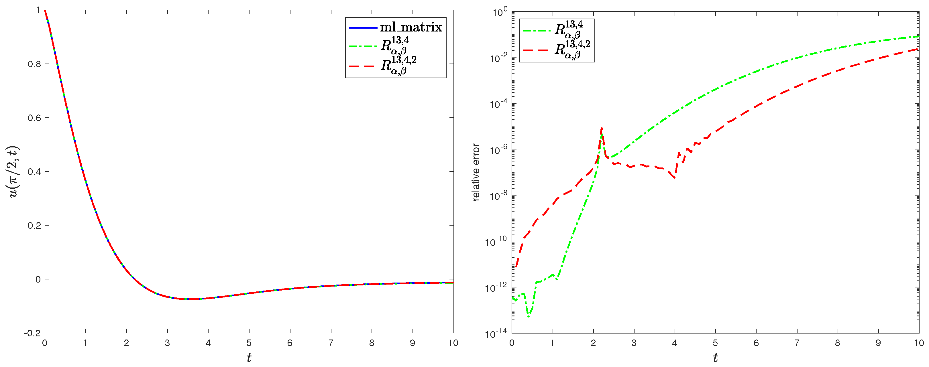
In Figure 13, the solution profile is presented for the case α = 1.2 . As can be seen, both the global Padé approximant R 1.2 , 1 13 , 4 and its generalization R 1.2 , 1 13 , 4 , 2 are comparable. This is expected since the solution has only one root, and not much oscillatory behavior is experienced. In Figure 14, the case α = 1.9 , where the MLF is more oscillatory, is presented. In this case, the rational approximant R 1.9 , 1 13 , 4 fails to capture the oscillations for large t and thus yields undesirable approximations. However, the modified R 1.9 , 1 13 , 4 , r with an appropriate choice r = 2 rectifies this issue and gives more accurate approximate values.
To illustrate the efficiency of these approximants, their runtimes are compared with that of the ml_matrix MATLAB function. Table 5 showcases the CPU times for computing the solution U ( t ) = E α ( A t α ) U 0 on a time mesh { t n = 0.1 n , n = 0 , 1 , 100 } . The results show that the approximant R 1.9 , 1 13 , 4 , 2 performs about seven times faster than the ml_matrix function. Moreover, while the approximant R 1.9 , 1 13 , 4 , 2 on an extended interval is able to achieve higher accuracy than R 1.9 , 1 13 , 4 , their runtimes are comparable.

7. Concluding Remarks

In this paper, a characterization of the oscillatory and monotone behavior of the two-parameter Mittag–Leffler function is given. Furthermore, generalized rational approximants over extended intervals are developed. These approximants are based on decomposing a Mittag–Leffler function that possesses real roots into a combination of a weighted rootless Mittag–Leffler function and a polynomial. The approximants have good tracking capabilities of the roots and oscillations over extended intervals. To show the efficiency of these approximants, numerical experiments are presented alongside various applications. Furthermore, to demonstrate computational efficiency, comparisons with the ml and ml_matrix MATLAB functions are included. Such approximants play an effective role in the implementation of numerical methods for fractional oscillation equations.

Author Contributions

Conceptualization, A.H.H. and K.M.F.; methodology, A.H.H., K.M.F. and I.O.S.; validation, A.H.H., K.M.F. and I.O.S.; writing—original draft preparation, A.H.H.; writing—review and editing, A.H.H., K.M.F. and I.O.S.; review and editing, A.Q.M.K. All authors have read and agreed to the published version of the manuscript.

Funding

This research received no external funding.

Data Availability Statement

Data are contained within the article.

Conflicts of Interest

The authors declare no conflicts of interest.

References

  1. Kilbas, A.; Srivastava, H.; Trujullo, J. Theory and Applications of Fractional Differential Equations; Elsevier: Amsterdam, The Netherlands, 2006. [Google Scholar]
  2. Gorenflo, R.; Kilbas, A.A.; Mainardi, F.; Rogosin, S.V. Mittag-Leffler Functions. Related Topics and Applications; Springer: Berlin/Heidelberg, Germany, 2014. [Google Scholar]
  3. Gorenflo, R.; Mainardi, F. Fractional Oscillations and Mittag-Leffler Functions; Citeseer: Berlin, Germany, 1996. [Google Scholar]
  4. Mainardi, F. Fractional relaxation-oscillation and fractional diffusion-wave phenomena. Chaos Solitons Fractals 1996, 7, 1461–1477. [Google Scholar] [CrossRef]
  5. Achar, B.N.; Hanneken, J.; Enck, T.; Clarke, T. Dynamics of the fractional oscillator. Phys. A Stat. Mech. Its Appl. 2001, 297, 361–367. [Google Scholar] [CrossRef]
  6. Stanislavsky, A. Fractional oscillator. Phys. Rev. E 2004, 70, 051103. [Google Scholar] [CrossRef] [PubMed]
  7. Stanislavsky, A.A. Twist of fractional oscillations. Phys. A Stat. Mech. Its Appl. 2005, 354, 101–110. [Google Scholar] [CrossRef]
  8. Gorenflo, R.; Loutchko, J.; Luchko, Y. Computation of the Mittag-Leffler function Eα,β(z) and its derivative. Fract. Calc. Appl. Anal. 2002, 5, 491–518. [Google Scholar]
  9. Garrappa, R. Numerical evalution of two and three parameter Mittag-Leffler functions. SIAM J. Numer. Anal. 2015, 53, 1350–1369. [Google Scholar] [CrossRef]
  10. Sarumi, I.O.; Furati, K.M.; Khaliq, A.Q.M. Highly Accurate Global Padé Approximations of Generalized Mittag–Leffler Function and Its Inverse. J. Sci. Comput. 2020, 82, 46. [Google Scholar] [CrossRef]
  11. Sarumi, I.O.; Furati, K.M.; Khaliq, A.Q.M.; Mustapha, K. Generalized Exponential Time Differencing Schemes for Stiff Fractional Systems with Nonsmooth Source Term. J. Sci. Comput. 2021, 86, 1–22. [Google Scholar] [CrossRef]
  12. Iyiola, O.S.; Asante-Asamani, E.O.; Wade, B.A. A real distinct poles rational approximation of generalized Mittag-Leffler functions and their inverses: Applications to fractional calculus. J. Comput. Appl. Math. 2018, 330, 307–317. [Google Scholar] [CrossRef]
  13. Starovoitov, A.P.; Starovoitova, N.A. Padé approximants of the Mittag-Leffler functions. Sb. Math. 2007, 198, 1011–1023. [Google Scholar] [CrossRef]
  14. Borhanifar, A.; Valizadeh, S. Mittag-Leffler-Padé approximations for the numerical solution of space and time fractional diffusion equations. Int. J. Appl. Math. Res. 2015, 4, 466. [Google Scholar] [CrossRef]
  15. Winitzki, S. Uniform Approximations for Transcendental Functions. In Computational Science and Its Applications, Proceedings of the ICCSA 2003: International Conference Montreal, Montreal, QC, Canada, 18–21 May 2003; Kumar, V., Gavrilova, M.L., Tan, C.J.K., L’Ecuyer, P., Eds.; Springer: Berlin/Heidelberg, Germany, 2003; pp. 780–789. [Google Scholar]
  16. Atkinson, C.; Osseiran, A. Rational solutions for the time-fractional diffusion equation. SIAM J. Appl. Math. 2011, 71, 92–106. [Google Scholar] [CrossRef]
  17. Zeng, C.; Chen, Y.Q. Global Padé approximations of the generalized Mittag-Leffler function and its inverse. Fract. Calc. Appl. Anal. 2015, 18, 1492–1506. [Google Scholar] [CrossRef]
  18. Ingo, C.; Barrick, T.R.; Webb, A.G.; Ronen, I. Accurate Padé global approximations for the Mittag-Leffler function, its inverse, and its partial derivatives to efficiently compute convergent power series. Int. J. Appl. Comput. Math. 2017, 3, 347–362. [Google Scholar] [CrossRef]
  19. Hanneken, J.W.; Vaught, D.M.; Achar, B. Enumeration of the Real Zeros of the Mittag-Leffler Function Eα(z), 1<α<2. In Advances in Fractional Calculus; Springer: Berlin/Heidelberg, Germany, 2007; pp. 15–26. [Google Scholar]
  20. Hanneken, J.W.; Achar, B.; Vaught, D.M. An alpha-beta phase diagram representation of the zeros and properties of the Mittag-Leffler function. Adv. Math. Phys. 2013, 2013, 421685. [Google Scholar] [CrossRef]
  21. Duan, J.S.; Wang, Z.; Fu, S.Z. The zeros of the solutions of the fractional oscillation equation. Fract. Calc. Appl. Anal. 2014, 17, 10–22. [Google Scholar] [CrossRef]
  22. Garrappa, R.; Popolizio, M. Computing the matrix Mittag-Leffler function with applications to fractional calculus. J. Sci. Comput. 2018, 77, 129–153. [Google Scholar] [CrossRef]
  23. Honain, A.H.; Furati, K.M. Rational Approximation for Oscillatory Mittag-Leffler Function. In Proceedings of the IEEE 2023 International Conference on Fractional Differentiation and Its Applications (ICFDA), Ajman, United Arab Emirates, 14–16 March 2023; pp. 1–5. [Google Scholar]
  24. Haubold, H.J.; Mathai, A.M.; Saxena, R.K. Mittag-Leffler functions and their applications. J. Appl. Math. 2011, 2011, 298628. [Google Scholar] [CrossRef]
  25. Podlubny, I. Fractional Differential Equations; Academic Press: Cambridge, MA, USA, 1999. [Google Scholar]
  26. Podlubny, I. 2009. Available online: www.mathworks.com/matlabcentral/fileexchange/8738 (accessed on 1 April 2024).
  27. Sadeghi, A.; Cardoso, J.R. Some notes on properties of the matrix Mittag-Leffler function. Appl. Math. Comput. 2018, 338, 733–738. [Google Scholar] [CrossRef]
  28. Higham, N.J. Functions of Matrices: Theory and Computation; SIAM: Philadelphia, PA, USA, 2008. [Google Scholar]
  29. Sastre, J. Efficient evaluation of matrix polynomials. Linear Algebra Its Appl. 2018, 539, 229–250. [Google Scholar] [CrossRef]
  30. Garrappa, R. Exponential integrators for time-fractional partial differential equations. Eur. Phys. J. Spec. Top. 2013, 222, 1915–1927. [Google Scholar] [CrossRef]
  31. Aguilar, J.G.; Hernández, J.R.; Jiménez, R.E.; Astorga-Zaragoza, C.; Peregrino, V.O.; Fraga, T.C. Fractional electromagnetic waves in plasma. Proc. Rom. Acad. A 2014, 17, 31–38. [Google Scholar]
  32. Murillo, J.Q.; Yuste, S.B. An explicit difference method for solving fractional diffusion and diffusion-wave equations in the Caputo form. J. Comput. Nonlinear Dyn. 2011, 6, 021014. [Google Scholar] [CrossRef]
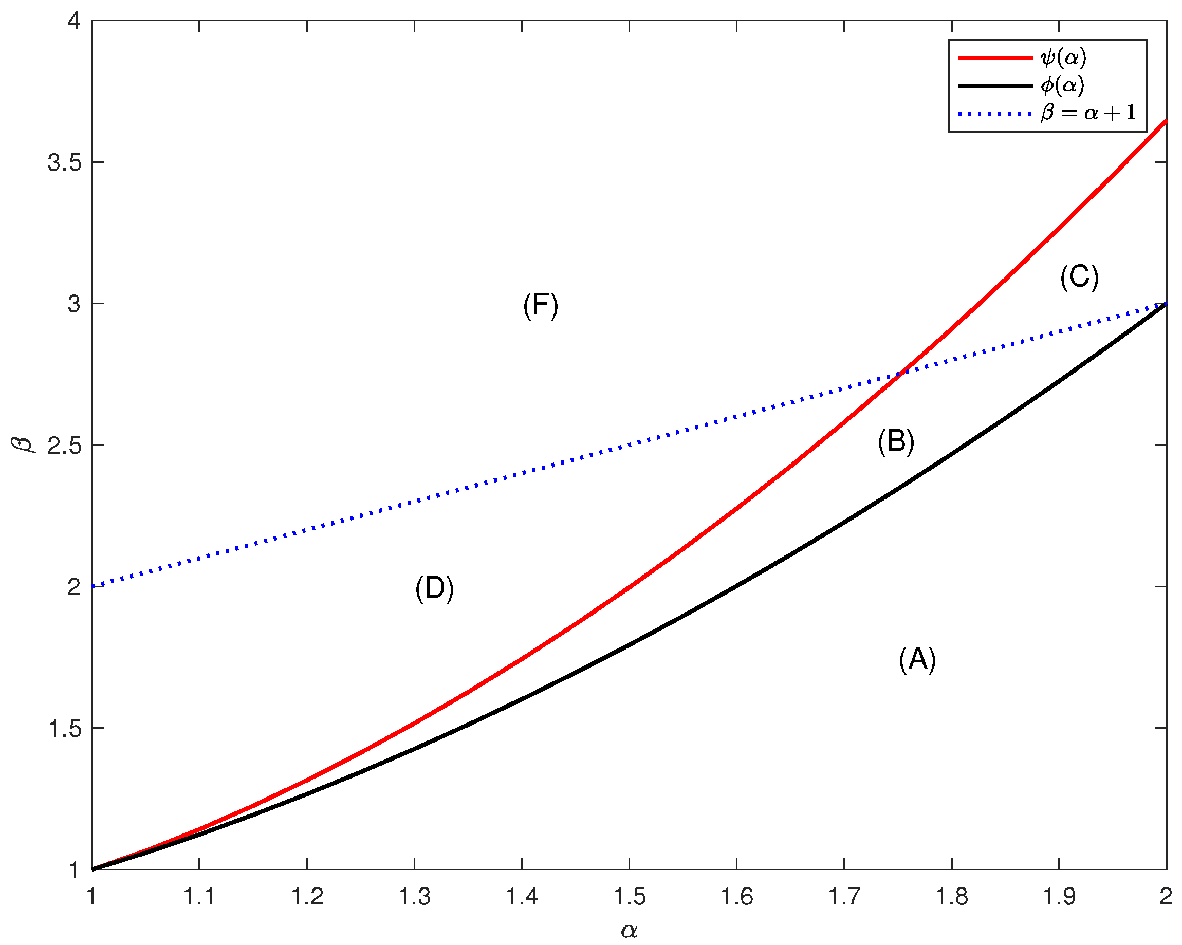
Figure 1. α - β phase diagram for E α , β ( t ) and its derivative, illustrating the function’s behavior for five distinct regions. In region (A), E α , β exhibits oscillatory behavior with the presence of real roots. In regions (B) and (C), E α , β oscillates without roots. In regions (D) and (F), E α , β displays monotonic behavior.
Fractalfract 08 00319 g001
Figure 2. Typical oscillations in region (B) about the roots (marked by the red lines) of the derivative.
Fractalfract 08 00319 g002
Figure 3. Plots of R α , β 13 , 4 and R α , β 7 , 2 approximants of E α , β when ( α , β ) is in region (A).
Fractalfract 08 00319 g003
Figure 4. Plots of R α , β 13 , 4 and R α , β 7 , 2 approximants of E α , β when ( α , β ) is in regions (B) and (C).
Fractalfract 08 00319 g004
Figure 5. Plots of R α , β 13 , 4 and R α , β 7 , 2 approximants of E α , β when ( α , β ) is in regions (D) and (F).
Fractalfract 08 00319 g005
Figure 6. Plots of R α , β 13 , 4 , r for different values of r when ( α , β ) is in region (A).
Fractalfract 08 00319 g006
Figure 7. Plots of R α , β 13 , 4 , r for different values of r when ( α , β ) is in region (C).
Fractalfract 08 00319 g007
Figure 8. Plots of R α , β 7 , 2 , r for different values of r when ( α , β ) is in region (A).
Fractalfract 08 00319 g008
Figure 9. MLF matrix approximation R α , β 13 , 4 , with ( α , β ) = ( 1.9 , 1 ) , of a 100 × 100 Redheffer matrix using partial fractions (left) and its relative error (right).
Fractalfract 08 00319 g009
Figure 10. Profiles (left) and relative error (right) in approximating the solution of (26), with α = 1.2 .
Fractalfract 08 00319 g010
Figure 11. Profiles (left) and relative error (right) in approximating the solution of (26), with α = 1.9 .
Fractalfract 08 00319 g011
Figure 12. Profiles (left) and relative error (right) in approximating the solution of (27), with α = 1.9 .
Fractalfract 08 00319 g012
Figure 13. Approximation of u ( π / 2 , t ) (left) and relative error (right), with α = 1.2 .
Fractalfract 08 00319 g013
Figure 14. Approximation of u ( π / 2 , t ) (left) and relative error (right), with α = 1.9 .
Fractalfract 08 00319 g014
Table 1. The data for the boundary ϕ ([20], Table 1) and the boundary ψ . The function E α , β possesses real roots below the curve ϕ ( α ) and has no real roots above it. Conversely, below the curve ψ ( α ) , E α , β exhibits non-monotonic behavior, whereas above it, the function demonstrates monotonicity.
α ϕ ( α ) ψ ( α )
1.00 1.00000 1.00000
1.05 1.05924 1.06640
1.10 1.12400 1.14204
1.15 1.19325 1.22532
1.20 1.26674 1.31565
1.25 1.34437 1.41277
1.30 1.42608 1.51654
1.35 1.51187 1.62689
1.40 1.60173 1.74374
1.45 1.69565 1.86706
1.50 1.79365 1.99685
1.55 1.89573 2.13306
1.60 2.00191 2.27568
1.65 2.11219 2.42471
1.70 2.22660 2.58014
1.75 2.34513 2.74196
1.80 2.46779 2.91017
1.85 2.59460 3.08477
1.90 2.72557 3.26575
1.95 2.86070 3.45311
2.00 3.00000 3.64686
Table 2. Number of roots in the regions in Figure 1.
Region E α , β ( t ) dE α , β / dt
AFinite number of rootsFinite number of roots
BNo real rootsFinite number of roots
CNo real rootsFinite number of roots
DNo real rootsNo real roots
FNo real rootsNo real roots
Table 3. Maximum absolute errors (AEs), maximum relative errors (REs), and runtimes (in seconds) for computing the matrix MLF of a 100 × 100 Redheffer matrix, with β = 1 .
α = 1.5 α = 1.9
AERERuntimeAERERuntime
Linear System 1.13 × 10 04 7.20 × 10 03 1.90 × 10 03 2.41 × 10 08 3.00 × 10 06 1.10 × 10 03
Partial Fraction 1.13 × 10 04 7.20 × 10 03 3.70 × 10 03 2.41 × 10 08 3.00 × 10 06 2.30 × 10 03
ml_matrix 1.44 × 10 01 9.73 × 10 + 00
Table 4. Maximum relative errors (REs) and runtimes for computing the solution for (26) over the time mesh [ 0 , 0.17 , 0.34 , , 10 ] , with α = 1.9 .
RERuntime
R α , β 13 , 4 3.00 × 10 01 5.69 × 10 04
R α , β 13 , 4 , 2 5.95 × 10 03 5.19 × 10 04
R α , β 13 , 4 , 5 2.23 × 10 06 5.20 × 10 04
R α , β 13 , 4 , 8 3.55 × 10 10 5.52 × 10 04
mL- 2.38 × 10 02
Table 5. Runtimes for computing the solution of (29) over the time mesh [ 0 , 0.1 , 0.2 , , 10 ] , with α = 1.9 .
Runtime
R 1.9 , 1 13 , 4 8.00 × 10 02
R 1.9 , 1 13 , 4 , 2 9.95 × 10 02
ml_matrix 6.70 × 10 01
Disclaimer/Publisher’s Note: The statements, opinions and data contained in all publications are solely those of the individual author(s) and contributor(s) and not of MDPI and/or the editor(s). MDPI and/or the editor(s) disclaim responsibility for any injury to people or property resulting from any ideas, methods, instructions or products referred to in the content.