Abstract
This research utilizes the innovative fractional-order Archimedean spiral moth–flame optimization (FO-AMFO) technique to address the issues of the optimal reactive power dispatch (ORPD) problem. The formulated fitness function aims to minimize power losses and determine the ideal flow of reactive power for the IEEE 30- and 57-bus test systems. The extensive functions of the fractional evolutionary computing strategy are utilized to address the minimization problem of ORPD. This involves determining the control variables, such as VAR compensators, bus voltages, and the tap setting of the transformers. The effective incorporation of reactive compensation devices into traditional power grids has greatly reduced power losses; however, it has resulted in an increase in the complexity of optimization problems. A comparison of the findings indicates that swarming fractional intelligence using FO-AMFO surpassed the state-of-the-art competitors in terms of minimizing power losses.
1. Introduction
The optimal reactive power dispatch (ORPD) problem is gaining attention from power system engineering researchers because of its importance in modern energy management systems. The objective is to minimize power losses in the electric power network and improve the net voltage profile and various equality and inequality constraints associated with the power system. Reactive power planning is an essential prerequisite for ensuring the dependable, efficient, and sustainable functioning of power systems as the power sector research community is increasingly intrigued by them [1,2,3]. We can accomplish these goals by finding the most accurate values of operational parameters including flexible AC transmission system (FACTS) devices, shunt reactor banks, generator voltages, tap positions of transformers and active power generation. Gradient-free solutions are very useful in terms of application in integrated power plants. The research community has become more familiar with metaheuristic methods and are using them in power system problems. Particle swarm optimization (PSO), a metaheuristic global technique inspired by nature, was employed to determine the optimal results for economic load dispatch (ELD) in conjunction with differential evolution (DE) for constructing hybrid energy-generating units [4]. Genetic algorithms (GAs) were employed to address the problem of ELD in conjunction with physical constraints when numerical methods failed to yield globally optimal outcomes. The enhanced genetic algorithm yielded more accurate and dependable results by meticulously organizing the outputs of active power generation [5]. Furthermore, the power and energy sectors have employed recently developed metaheuristic-based searching algorithms, as detailed in [6]. Mirjalili’s [7] biologically inspired meta heuristic strategy of grey wolf optimization (GWO) is an intriguing methodology that may be applied to challenging real-world ELD problems. GWO is used to solve many common optimization issues. Complex power system problems were solved using quadratic programming, linear programming, dynamic programming, the Newton–Raphson method, and sequential programming. However, because of convergence issues and initial search point sensitivities [8], these traditional optimization techniques are unable to yield global optimum results. The combination of several optimization strategies is promising and has produced the finest all-around results. Hybridization approaches promise the finest global solutions by simultaneously utilizing the best aspects of individual algorithms [9]. Several practical constraints, such as power demands, generation limits, emissions, prohibited operating zones (POZs), multi-fuel systems, limits to ramp rates, the stochastic behavior of renewable energy penetration, bus voltages, tap changer transformers, reactive power compensators, and multiple controlled continuous, discrete, and integer-based variables, are involved in addressing the various objectives of power systems. These problems are highly nonlinear and non-convex optimization problems [10]. Because of stagnation in local optimal zones, traditionally employed optimization strategies face more challenges in the proper planning, operation, and management of power plants. A useful substitute for solving challenging power system optimization issues is bio-inspired methods. Bio-inspired algorithms are more likely to broaden the search space and have less chance of becoming trapped in local optimum regions because of their stochastic and population-based nature compared to deterministic techniques, which evaluate search agents using function derivatives rather than fitness functions [11]. Among the broad categories of bio-inspired algorithms are those based on ecology, swarming, and evolutionary optimization. Hybrid bio-inspired algorithms benefit from the ability to simultaneously find the optimum solution without getting entrapped in the wrong zones. An important component of power system optimization is the problem of economic load and emissions, which has been successfully solved to optimize fuel cost generation and the amount of harmful gas emissions [12]. By taking into account the valve point loading effect (VPLE), prohibited operations zones (POZs), and multiple fuel options for test systems with 10, 40, and 160 units, the author solved a multi-objective problem which optimizes power generation fuel costs, emission of gases, and power losses in transmission lines, linked to the ELD problem [13], by formulating a fuzzy-based PSO hybrid method with DE, called FB (PSO-DE). By comparing the performance of the suggested combined technique to PSO with more then seven limited benchmark functions derived from 100 separate trials, the hybrid strategy demonstrated improved robustness and convergence compared to PSO and its various hybrid approaches. In order to minimize the fuel generation cost while taking the VPLE into consideration, the continuous greedy randomized adaptive search procedure algorithm (GRASP) is employed in combination with self-adaptive differential evolution, denoted CGRASP-SADE [14]. ELD with incorporation of wind power units is discussed in [15], in which the moth–flame optimization (MFO) algorithm was used for cost minimization. In [16], the optimal power flow problem is approached by applying fractional-order computing via variations of FO-PSO. This involves determining control variables, including VAR compensators, generator bus voltages, and tap setting of transformers. The author used the DE algorithm in [17] to address power loss minimization for nonlinear and piecewise second-order cost functions. Comprehensive learning particle swarm optimization (CL-PSO) for reactive dispatch of an IEEE-30 bus system is used in [18]. The harmony search algorithm’s ability to handle inequality constraints and penalty coefficients is studied in [19]. The hybrid invasive weed algorithm combined with the implicit competitive algorithm is used for IEEE 30- and 57-bus systems in [20]. The quasi oppositional algorithm [21] is used for loss minimization of large IEEE 118-bus systems. The grey wolf optimizer (GWO) is used to find the optimum parameter settings for an IEEE 57-bus system in [22]. In [23] Optimal reactive power dispatch solution by loss minimization is solved using moth flame optimizer. In traditional MFO, during the last iteration of optimization, almost all individuals in the population converge to a small region around the optimal solution. When faced with intricate multimodal global optimization issues, the whole population may quickly converge to the local optimum. In order to address this problem, a modified version of MFO called the FO-AMFO method is proposed. This modified version incorporates the concept of fractional calculus to improve the convergence characteristics and capabilities of MFO.
Recently, it has been established that incorporating fractional calculus (FC) and the fundamental notions of fractional derivatives into a system’s underlying mathematical model can provide considerably better outcomes in various fields of science and engineering. These approaches have been successfully applied to a wide range of problems, including feature selection, image processing, hyperspectral visuals, controllers for predicting robotic paths, Kalman filters, and fractional-order filters. According to this study, FC techniques should be used with evolutionary strategies to address optimization difficulties in the energy sector. We can refer to fractional-order robotic PSO, FPSO with a fractional-order velocity [24,25,26,27,28], optical disc localization and segmentation [29], parameter adaptation for Kalman filtering computations [30], land-cover tracking [31], feature selection [32], hyperspectral image classification [33], and robot path controller design [34]. Other applications involve the development of a multiband power system stabilizer based on a lead–lag compensator using hybrid dynamic GA-PSO [35] and identification of nonlinear systems [36]. These findings encourage the use of FC tools in conjunction with metaheuristic algorithms to solve the energy and power sectors’ optimization challenges.
The use of fractional-order calculus in the AMFO algorithm demonstrates the synergistic convergence of complex optimization approaches. FO-AMFO’s inherent fractal-order dynamics boost exploration and exploitation capabilities, allowing for more effective ORPD problem optimization. The addition of fractional calculus to the AMFO algorithm improves the accessibility, consistency, and scalability of the optimization process. ORPD allows for the automated application and enforcement of optimization criteria, which simplifies energy dispatch operations and lowers power losses. Furthermore, the integration of FO-AMFO in ORPD has the potential to drive innovation in energy-market procedures and grid management strategies. FO-AMFO enabled ORPD for real-time optimization and dynamic changes in energy loads, resulting in improved resource utilization, lower energy costs and power losses, and improved grid stability. The performance of FO-AMFO is heavily impacted by parameter configurations such as the fractional order, inertia weights, and acceleration coefficients. Inadequate parameter settings may cause early convergence, a lack of progress, or erratic behavior, necessitating careful parameter modification and optimization.
The aim of this research work is to solve the constrained optimization problem of ORPD. According to our literature study, the potential of FO-AMFO-based heuristics has not been applied to ORPD so far. Thus, this study investigates the potential for optimizing the algorithms in ORPD.
This article describes the application of FO-AMFO, a recently developed variant of the MFO algorithm that emphasizes the concepts and theories of fractional calculus. It serves as an effective mechanism for optimizing ORPD by estimating control variables, such as bus voltages, tap positions of transformers, and reactive power compensators, while satisfying the load demand. As a fitness evaluation function, power loss minimization is employed, while keeping the constraints within their designated bounds. The important characteristics, or highlights of the contributions, are listed as:
- Utilizing the strengths of FO-AMFO, a novel application of the fractional evolutionary approach for ORPD is proposed.
- The design scheme is successfully applied to ORPD problems in order to minimize power losses while meeting load demand and operational constraints.
- The algorithm’s performance is determined by statistical findings in the form of probability plots, learning curves, and histogram analysis, which demonstrate the algorithm’s stability, resilience, and consistency as a precise and efficient optimization mechanism.
The remainder of the paper has been drafted in following order: Section 2 presents the fitness function for ORPD problem; Section 3 presents a summary of the proposed FO-AMFO method and the overall flow diagram; Section 4 presents the simulation results and a comparison with the latest techniques applied to same problem; and Section 5 presents the conclusions and future recommendations.
2. Problem Formulation
ORPD is an essential part of controlling and managing power systems. Its primary goal is to meet various constraints while minimizing power losses. Efficient distribution of electrical energy within the power grid is the goal of ORPD. The overarching goal is to lower the system’s overall cost, which includes factors like power losses and voltage deviations.
Our primary goal is to reduce the power losses related to the standard IEEE networks. The actual power dissipation of the system is determined by the bus voltages, corresponding angles and line conductances, expressed mathematically by:
Here, δ are the voltage phasor angles at the i and j buses, whereas e represents the line, w represents the transmission system, grr represents the transmission line conductance, and Vii and Vjj are the magnitude of the bus voltages. It is also crucial to note that the reactance of the line varies with the transformer tap setting (T) and the voltage of the bus in relation to the complex part of power (Q).
Furthermore, the penalty factor approach has been included to penalize the control variable violations because, in ORPD situations, if the control variables exceed the voltage constraints, significant harm to the power network will occur. The penalty factor term is zero if every control variable stays within the allowed ranges. Thus, the objective function becomes the equation below.
is the penalty factor function and rg and rh are the penalty multipliers for constraints.
X represents the set of independent variables = xi ϵ [V, T, Q]. It comprises the IEEE standard bus system’s Qi (capacitor bank), the voltage control bus Vi, and the transformer tap setting Ti. The total objective function that takes into account the penalty function for breaking both constraints is
In this case, the variables V, Q, and T represent the generator bus voltages, reactive power, tap locations, generator numbers (NG), and total tap changers (NT). The upper and lower, or permissible, limits of these control variables are represented by the highest and lowest values of Qi, Vi and Ti in the aforementioned equations. Equation (3) states that any deviation from these bounds will result in a fitness penalty.
2.1. System Constraints
Power balancing equations, as given in [10], are the equality constraint in power flow, stating that losses in the power system are equal to the difference between the generation and demand of power at each bus. The following are mathematical equations for both real and reactive powers:
The actual power supply and demand at the ith bus are denoted by PGi and PDi, respectively, whereas the reactive power generation and demand at the ith bus are represented by QGi and QDi. Bij and Gij are the line’s conductance and susceptance.
The inequality constraints used are given below.
2.2. Tap Limits
The tap positions of transformers are denoted as:
2.3. Voltage Generation Limits
The upper and lower voltage generation limits are:
2.4. Reactors Limits
The compensators at the bus are limited by:
Here, the total number of branches si NT, the total number of generators si N and buses with compensators are represented by NC.
3. Methodology
The approach here to address the ORPD problem for IEEE-30 and IEEE-57 bus systems is based on FO-AMFO. Two sections are devoted to the description of the design plan. The first section gives a quick rundown of FO-AMFO and its derivation. The second section then presents the general workflow for solving the ORPD problem using basic steps and processing block structures. In this part, an original method for improving the classic MFO algorithm’s local search approach is presented. First, to develop the MFO approach, Mirjalili [37] was motivated by the transverse positioning of moths during nocturnal navigation. Unlike other nature-inspired algorithms, MFO employs spiral trajectory functions to mathematically model dying behavior. By maintaining a steady angle with the moonlight, and in order to facilitate more effective nocturnal migration over great distances, moths use transverse orientation as a navigational strategy, as shown in Figure 1a. When moths encounter artificial lights or flames during the night, they tend to bend away from the original path; this is the reason behind moths randomly moving in arbitrary directions. Moths perish as they fall into artificial light because of deadly spiral orientation, as shown in Figure 1b, which shows an Archimedean spiral trajectory.
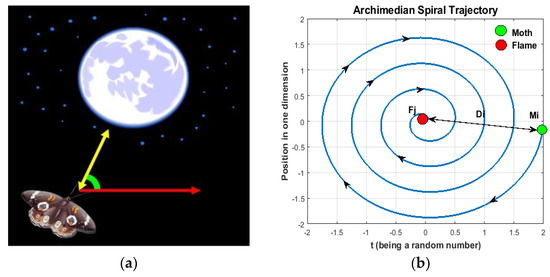
Figure 1.
FO-AMFO: (a) moth–flame inspiration; (b) moth trajectory.
The population-based MFO algorithm is a type of search algorithm. Each moth functions as a search agent in this system, and its orientation indicates the number of variables that may be controlled. The goal of this strategy is to identify the best options. The first solution for moths, called “M”, is included in the framework. It is composed of “n” candidate solutions and “d” dimensions, which stand for controllable variables. The matrix ‘OM’ represents the fitness of these potential solutions, which is assessed using an objective function.
For flames, a matrix ‘F’ is designed, which is dimensionally the same as that observed for moths. ‘OF’ stands for the fitness-encoded values in the matrix. Moths select the best location, and subsequently, search agents modify their positions based on the optimal position obtained.
Every nth moth’s location in relation to the kth flame is altered using the ‘S’ spiral function.
The Archimedean spiral function is used by modifying the MFO method to mimic the flight of moths in spiral paths, and Equation (14) is used to improve the alignment. The straight distance between the kth and the nth moth is represented by the variable “Dn”. In this case, ‘r’ is a randomly generated value between −1 and 1, and ‘k’ is the logarithmic spiral’s form factor.
The suggested approach combines fractional calculus with the previously mentioned basic MFO to provide fractional-order MFO that controls the propensity toward faster convergence and yields satisfactory outcomes. MFO works well with global search methods, whereas its performance is not good in local search methods. To avoid the previously described restriction, the suggested approach incorporates fractional calculus into basic MFO to make use of the memory retention feature of previous solutions to ensure information exchange between solutions throughout the solution phase. As a result, modifications are made to the convergence speed and response accuracy. Given its properties and intrinsic memory component, FC is ideally equipped to explain fascinating phenomena like irreversibility and chaos. This theory states that an MFO trajectory’s dynamic character produces a special circumstance, while FC instruments are a good complement.
The concept of fractional-order derivatives is formulated by applying fractional-order derivatives to Grünwald–Letnikov theory. Take any random signal s(t), for which Equation (15) provides the fractional-order derivative of Grünwald–Letnikov [38].
The fractional derivative requires infinite terms to represent it, whereas an integer derivative is simply represented by finite series. Therefore, “local” operators are derivatives of integers. Fractional derivatives, on the other hand, automatically “remember” every past event. Still, the impact of earlier occurrences fades with time. The expression found in Equation (16) serves as the basis for the discrete time computation.
where “r” denotes the truncation order and “T” denotes the sampling period. [s(t)] is a discrete variable. In the particular case where δ equals one, the equation can be stated as follows where it is changed to integer order or the conventional first-order derivative:
To leverage the property of fraction calculus that was discussed earlier to improve the local search capabilities of conventional moth–flame optimization, each moth’s position is updated according to the velocity in Equation (18).
Moths move in a PSO fashion, where the best flame (GBFPOS) is the global optimum and the moth-associated flame (LBFPOS) is the local best position. Every iteration updates each moth’s position based on its current position and velocity. The updated velocity is in line with the moth’s initial velocity as well as social behavior patterns and cognitive processes.
The main idea of the proposed FO-AMFO algorithm is shown in Figure 2.

Figure 2.
Flowchart of the complete process.
Considering only four terms, Equation (20) can be rewritten as follows.
4. Results and Discussion
It is common practice to evaluate the performance of an optimization method via standard uni- and multi-model benchmark functions [37]. The approximate solution with the lowest error is considered to be the best optimizer. A total of 10 benchmark functions are used here for the comparison of optimization methods in different scenarios. First, the functions from F1 to F7 are uni-model functions, while F8 to F10 are multi model functions. F0-AMFO gives the best results in 8 cases out of 10 different test cases. The numerical outcomes are shown in Table 1, which shows F0-AMFO’s performance in terms of the mean fitness value among 100 independent runs. FO-AMFO outperformed all three algorithms.

Table 1.
Performance comparison with benchmark functions.
The numerical results obtained through FO-AMFO for solving ORPD problems are presented in this section, which includes two case studies of a 30-bus IEEE system with 13 variables to control and a 57-bus IEEE system with 25 variables to control. The parameter values of the system can be found in [16].
4.1. Case 1: ORPD 13 Variables for a 30-Bus IEEE System
In this case, FO-AMFO is applied to a 30-bus IEEE system; a detailed single-line diagram is shown in Figure 3. In this case, there are in total thirteen control variables—three compensator devices, four tap changer transformers, and six generator voltages—that need to be optimized for this case study. The system description data are given in Table 2.

Figure 3.
IEEE 30-bus system [16].

Table 2.
Description of IEEE 30 standard systems [16].
The actual and reactive power demands are taken from IEEE base case, but the optimization variables’ boundary limitations are different, as determined by [16]. In order to ensure a fair comparison, the same MATPOWER load flow numerical computational paradigm is used to evaluate all of the tabulated results of transmission losses. The results obtained by the proposed optimization technique in contrast to other optimization techniques are shown in Table 3, which demonstrate that FO-AMFO obtained a good-quality solution and minimized the total power losses up to the optimum value.

Table 3.
Comparison of 13 control variables for the IEEE 30-bus system.
Table 3 shows that the loss obtained by applying FO-AMFO is 4.2193 MW, which is 23.03% less than the base case loss of 5.482 MW. In contrast, MFO, MICA-IWO, GWO, DE, GA and HSA exhibit 18.6%, 14.4%, 18.5%, 13.6%, 13.8% and 9.7% lower losses, respectively, when compared to other recently established counterpart computational paradigms. The results show that while solving the optimal RPD problem, the FO-AMFO technique produces a superior solution to other well-known published techniques. Additionally, it is evident that every calculated result for an optimization variable stayed inside the predetermined bounds.
By examining the convergence and learning curves, as shown in Figure 4 and Figure 5, it is shown that the convergence is faster and the optimum solution is obtained in a fewer number of iterations during the course of the simulation. Further, it is shown from learning curve that after 23 iterations, the power loss seems to converge at a constant 4.2 MW value also for the case of fractional values, which reaches its peak performance at α = 0.3. From this, one can assess the resilience of FO-AMFO’s performance. The convergence curves were plotted for various fraction orders, i.e., for α = 0.10 to 0.90, with 0.10 difference in the computational scheme to observe the consistency in accuracy. The convergence curves for different fractions ranging from 0.1 to 0.9 in the case of the IEEE 30-bus system are shown in Figure 5. The X axis represents the iteration value and the Y axis represents the total power loss in the system. As the number of iterations increases, the convergence curve converges to a single solution. From Figure 5, it can be concluded that the fractional order α = 0.3 solution converges to 4.2 MW, which is the best value recorded. It can be seen that after 100 iterations, the exploration step is lowest and the exploitation step is prominent.

Figure 4.
Convergence characteristics for FO-AMFO for case 1.
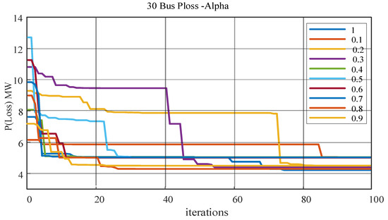
Figure 5.
Convergence curves for α = 0.1 to 0.9 for case 1.
Figure 6 shows the loss difference obtained by applying FO-AMFO, which is 5.482 MW, which can also be interpreted as a 1.2627 MW power loss difference from the base case of 5.482 MW. The power loss difference is obtained by subtracting the power loss obtained by the optimization method from the base case power loss. In the same way, MFO, MICA-IWO, GWO, DE, GA and HSA exhibit differences of 0.874 MW, 0.869 MW, 0.636 MW, 0.5945 MW and 0.37 MW when compared to other recently established similar computational paradigms.
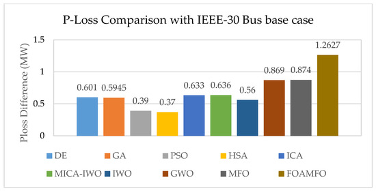
Figure 6.
P-Loss comparison with the IEEE 30-bus base case.
4.2. Case 2: ORPD for the IEEE 57-Bus System with 25 Control Variables
In this case, the proposed FO-AMFO is applied to the IEEE 57-bus system, as shown in Figure 7. In this case, there are a total of twenty-five variables. The system details anc be found in [16]. The system parameters and description data for the IEEE 57-bus standard system are shown in Table 4.
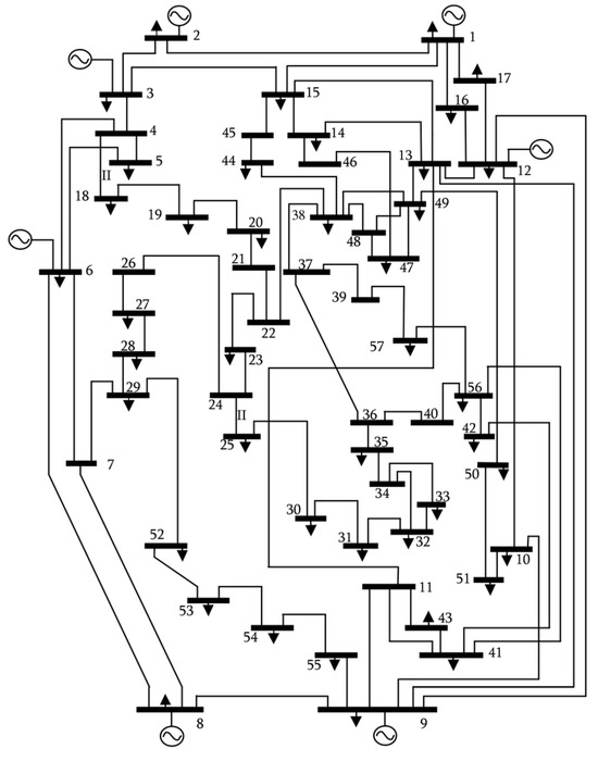
Figure 7.
IEEE 57-bus system [20].

Table 4.
Description of the IEEE 57-bus standard system [20].
The actual and reactive power demands are the same as in the previous case, but the optimization variable boundary limitations are different, as determined by [16]. The results obtained from the proposed FO-AMFO are compared with those of other well-known optimization methods and mentioned in Table 5. It can be observed that the proposed algorithm obtained a better and superior solution in terms of the quality of the solution and convergence characteristics and minimized the power line losses up to the optimum value. In order to ensure a fair comparison, the same MATPOWER load flow numerical computational paradigm was used to evaluate all of the tabulated results of transmission losses. Table 5 shows that the loss obtained by applying FO-AMFO is 21.6210 MW, which is 21.73% less than the base case loss of 27.86 MW. In contrast, FO-DPSO, SOA, MFO, IWO, CLPS, GWO and FPSO-GSA exhibit 4.23%, 12.92%, 11.72%, 10.66%, 12.66%, 14.44%, and 17.73% lower losses, respectively, when compared to other recently established similar computational paradigms. The results show that while solving the ORPD problem, the FO-AMFO technique produces a superior solution compared to other well-known published techniques. Additionally, it is evident that every calculated result for an optimization variable stayed inside the predetermined bounds.

Table 5.
Comparison of optimized variables for the IEEE 57-bus system with 25 control variables.
By examining the learning curve, which reaches its peak performance at α = 0.8, one can assess the resilience of FO-AMFO’s performance, as shown in Figure 8. The learning curves are also plotted for various fractional orders, i.e., for α = 0.1 to 0.9, in the computational scheme to observe the consistency, as shown in Figure 9 and Figure 10. It can be observed from the convergence and learning graph that the proposed FO-AMFO achieved the optimum solution and minimized the losses up to the optimum value in a lower number of iterations. The net gain improvement in power loss achieved in MWs by the proposed algorithm against the IEEE 30-bus base case with other optimization techniques is shown in Figure 9, demonstrating the superiority of FO-AMFO.

Figure 8.
Convergence characteristics of FO-AMFO for case 2.
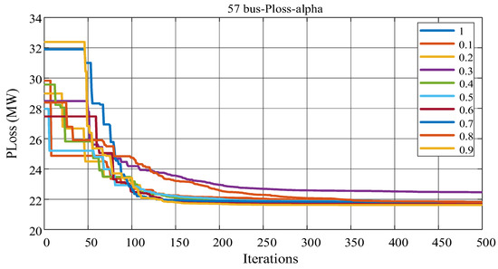
Figure 9.
Convergence curves for α = 0.1 to 0.9 for case B.
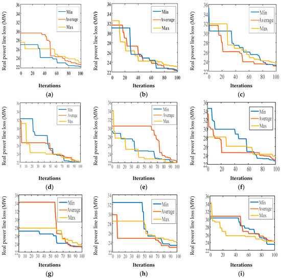
Figure 10.
Convergence characteristic curves of the proposed FO-AMFO algorithm for fractional orders of 0.1 to 0.9: (a) fractional order δ = 0.1, (b) fractional order δ = 0.2, (c) fractional order δ = 0.3, (d) fractional order δ = 0.4, (e) fractional order δ = 0.5, (f) fractional order δ = 0.6, (g) fractional order δ = 0.7, (h) fractional order δ = 0.8, (i) fractional order δ = 0.9.
The power losses for the IEEE 57-bus system and convergence curves for different fractions ranging from 0.1 to 0.9 are shown in Figure 9. The best value of Ploss among 20 independent trials and 500 iterations is shown, where the x axis represents the iteration value and the y- axis represents the power loss. As the number of iterations increases, the convergence curve flattens to a single solution. The fractional order value of α = 0.8 converges to 21.6210 MW, which is the lowest value. It can be seen that after 100 iterations, the exploration step is lowest and the exploitation step is prominent. The Figure 10 shows the minimum, average and maximum value obtained for real power losses obtained during the course of simulation for different fractional orders while Figure 11 shows the loss difference obtained by applying FO-AMFO as it can be seen the proposed FOAMFO achieved a Power loss difference of 6.239MW as compared to base case of IEEE-57 Bus system.
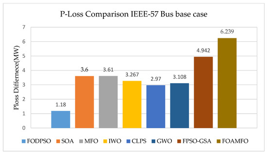
Figure 11.
P-Loss comparison with the IEEE 57-Bus base case.
4.3. Comparative Analysis through Statistics
In this section, the statistical analysis results are presented so that reliable conclusions can be drawn regarding the proposed FO-AMFO technique, which has been evaluated across 20 independent trials. The outcomes of the statistical analysis are presented, enabling reliable conclusions to be drawn concerning the FO-AMFO method, which was specifically developed to address the difficulty of determining the optimal ORPD. Box plots can represent the spread of data graphically. With respect to measurements of the central tendency (mean, median, and mode), the box plot for power loss minimization in Figure 12b reveals that the median and outliers are quite near to each other, which suggests a relatively low variation in the data. The shape of the computed data is reflected in the underlying frequency distribution, which is represented by the histogram drawings. It is evident that the maximum number of independent trials yields average minimum fitness gauges for every scenario. As can be observed, even the worst-case scenario offers a higher fitness value compared to the base case, verifying FO-AMFO’s accuracy. These visual representations of the statistical data for the various ORPD scenarios further demonstrate the consistency, stability, and robustness of FO-AMFO as a trustworthy and successful alternative optimization method in the energy sector. The data are presented in the form of probability graphs of the cumulative distribution function (CDF) in Figure 12a, which illustrate the line loss profiles for the most favorable scenarios. These graphs demonstrate that FO-AMFO optimizes the fitness functions consistently. The data are presented in the form of histograms in Figure 12a. The corresponding box plot results for bus 57 are shown in Figure 12b. The IEEE 57-bus system exhibits the minimal standard deviation and median values of 4.84 s across its 25 control variables. It is observed that the complexity parameter for an IEEE 57-bus system comprising 13 control variables does not exhibit any noticeable variation. In fact, as the number of degrees of freedom increases, the optimization problem becomes more challenging. In the overwhelming majority of FO-AMFO studies, the minimal measurements of actual power line losses are obtained. Multiple trials, when conducted independently, yield empirical power line loss values for the IEEE 57-bus system that are inferior to the most recent values reported in the literature. The obtained outcomes align with the CDF probability plots. The box plot drawings presented in Figure 12b illustrate the data, and suggest that the median value of line losses for the IEEE 57-bus system is approximately 21.62 MW.

Figure 12.
Statistical performance in terms of a histogram, a box plot and independent runs. (a) Histogram analysis. (b) Box plot for fitness. (c) Fitness comparison.
5. Conclusions
In order to solve RPD problems, this work proposed and tested FO-AMFO, a recently established fractional evolutionary optimization mechanism. The optimization method works well with every IEEE standard bus system that is taken into consideration. When compared to other cutting-edge meta-heuristics, the results show that the applied scheme performs better than its competitors in terms of minimizing the loss and ensuring the optimum reactive power. Different fractional-order values are used to create FO-AMFO variants, each of which is applied to both ideal RPD systems with a fair degree of precision. However, the scheme with a fractional order of 0.3 achieves a comparatively superior performance for the IEEE 30-bus system. The algorithm is consistent, robust, and stable as an alternative, accurate, and effective optimization mechanism for all cases of optimal RPD systems, as demonstrated by the statistical results in the form of learning curves, histogram studies, and probability plots based on 20 independent trials of FO-AMFO with α = 0.3. There is no discernible difference in the IEEE 30-bus system with 13 control variables. Also, for the 57-bus system, an alpha of 0.8 performs best according to the complexity of FO-AMFO for the solutions of optimal RPD problems in 20 independent trials.
Future research on the optimal RPD problem may involve developing fractional comprehensive learning MFO and fractional attributed comprehensive learning MFO algorithms. Furthermore, for nonlinear problems, the suggested FO-AMFO algorithms provide a promising substitute optimization strategy.
Author Contributions
Conceptualization, A.W.; Data curation, B.S.K.; Formal analysis, B.S.K.; Funding acquisition, S.B.R.; Investigation, E.A.; Methodology, A.W.; Project administration, S.B.R. and B.S.K.; Resources, B.S.K.; Software, E.A.; Supervision, A.W. and S.B.R.; Validation, E.A.; Visualization, A.W. and S.B.R.; Writing—original draft, E.A.; Writing—review and editing, A.W. All authors have read and agreed to the published version of the manuscript.
Funding
This research received no external funding.
Data Availability Statement
The data that support the findings of this study are available upon reasonable request from corresponding author.
Conflicts of Interest
The authors declare no conflicts of interest.
References
- Yu, X.; Yu, X.; Lu, Y.; Sheng, J. Economic and emission dispatch using ensemble multi-objective differential evolution algorithm. Sustainability 2018, 10, 418. [Google Scholar] [CrossRef]
- Jiang, S.; Ji, Z.; Wang, Y. A novel gravitational acceleration enhanced particle swarm optimization algorithm for wind–thermal economic emission dispatch problem considering wind power availability. Int. J. Electr. Power Energy Syst. 2015, 73, 1035–1050. [Google Scholar] [CrossRef]
- Jadoun, V.K.; Pandey, V.C.; Gupta, N.; Niazi, K.R.; Swarnkar, A. Integration of renewable energy sources in dynamic economic load dispatch problem using an improved fireworks algorithm. IET Renew. Power Gener. 2018, 12, 1004–1011. [Google Scholar] [CrossRef]
- Santra, D.; Sarker, K.; Mukherjee, A.; Mondal, S. Combined economic emission and load dispatch using hybrid metaheuristics. Int. J. Hybrid Intell. 2019, 1, 211–238. [Google Scholar] [CrossRef]
- Sinha, N.; Chakrabarti, R.; Chattopadhyay, P. Evolutionary programming techniques for economic load dispatch. IEEE Trans. Evol. Comput. 2003, 7, 83–94. [Google Scholar] [CrossRef]
- Gopalakrishnan, R.; Krishnan, A. An efficient technique to solve combined economic and emission dispatch problem using modified Ant colony optimization. Sadhana 2013, 38, 545–556. [Google Scholar] [CrossRef]
- Faris, H.; Aljarah, I.; Al-Betar, M.A.; Mirjalili, S. Grey wolf optimizer: A review of recent variants and applications. Neural Comput. Appl. 2017, 30, 413–435. [Google Scholar] [CrossRef]
- Manton, J. Optimization algorithms exploiting unitary constraints. IEEE Trans. Signal Process. 2002, 50, 635–650. [Google Scholar] [CrossRef]
- Hu, Y.; Liu, K.; Zhang, X.; Su, L.; Ngai, E.; Liu, M. Application of evolutionary computation for rule discovery in stock algorithmic trading: A literature review. Appl. Soft Comput. 2015, 36, 534–551. [Google Scholar] [CrossRef]
- Askarzadeh, A. Solving electrical power system problems by harmony search: A review. Artif. Intell. Rev. 2016, 47, 217–251. [Google Scholar] [CrossRef]
- Binitha, S.; Sathya, S.S. A survey of bio inspired optimization algorithms. Int. J. Soft Comput. Eng. 2012, 2, 137–151. [Google Scholar]
- Zhang, J.; Wu, Y.; Guo, Y.; Wang, B.; Wang, H.; Liu, H. A hybrid harmony search algorithm with differential evolution for day-ahead scheduling problem of a microgrid with consideration of power flow constraints. Appl. Energy 2016, 183, 791–804. [Google Scholar] [CrossRef]
- Naderi, E.; Azizivahed, A.; Narimani, H.; Fathi, M.; Narimani, M.R. A comprehensive study of practical economic dispatch problems by a new hybrid evolutionary algorithm. Appl. Soft Comput. 2017, 61, 1186–1206. [Google Scholar] [CrossRef]
- Neto, J.X.V.; Reynoso-Meza, G.; Ruppel, T.H.; Mariani, V.C.; dos Santos Coelho, L. Solving non-smooth economic dispatch by a new combination of continuous GRASP algorithm and differential evolution. Int. J. Electr. Power Energy Syst. 2017, 84, 13–24. [Google Scholar] [CrossRef]
- Khan, B.S.; Raja, M.A.Z.; Qamar, A.; Chaudhary, N.I. Design of moth flame optimization heuristics for integrated power plant system containing stochastic wind. Appl. Soft Comput. 2021, 104, 107193. [Google Scholar] [CrossRef]
- Muhammad, Y.; Khan, R.; Ullah, F.; Rehman, A.U.; Aslam, M.S.; Raja, M.A.Z. Design of fractional swarming strategy for solution of optimal reactive power dispatch. Neural Comput. Appl. 2019, 32, 10501–10518. [Google Scholar] [CrossRef]
- El Ela, A.A.; Abido, M.A.; Spea, S.R. Differential evolution algorithm for optimal reactive power dispatch. Electr. Power Syst. Res. 2011, 81, 458–464. [Google Scholar] [CrossRef]
- Mahadevan, K.; Kannan, P. Comprehensive learning particle swarm optimization for reactive power dispatch. Appl. Soft Comput. 2010, 10, 641–652. [Google Scholar] [CrossRef]
- Khazali, A.; Kalantar, M. Optimal reactive power dispatch based on harmony search algorithm. Int. J. Electr. Power Energy Syst. 2011, 33, 684–692. [Google Scholar] [CrossRef]
- Ghasemi, M.; Ghavidel, S.; Ghanbarian, M.M.; Habibi, A. A new hybrid algorithm for optimal reactive power dispatch problem with discrete and continuous control variables. Appl. Soft Comput. 2014, 22, 126–140. [Google Scholar] [CrossRef]
- Mandal, B.; Roy, P.K. Optimal reactive power dispatch using quasi-oppositional teaching learning based optimization. Int. J. Electr. Power Energy Syst. 2013, 53, 123–134. [Google Scholar] [CrossRef]
- Sulaiman, M.H.; Mustaffa, Z.; Mohamed, M.R.; Aliman, O. Using the gray wolf optimizer for solving optimal reactive power dispatch problem. Appl. Soft Comput. 2015, 32, 286–292. [Google Scholar] [CrossRef]
- Mei, R.N.S.; Sulaiman, M.H.; Mustaffa, Z.; Daniyal, H. Optimal reactive power dispatch solution by loss minimization using moth-flame optimization technique. Appl. Soft Comput. 2017, 59, 210–222. [Google Scholar] [CrossRef]
- Ghamisi, P.; Couceiro, M.S.; Benediktsson, J.A. A Novel Feature Selection Approach Based on FODPSO and SVM. IEEE Trans. Geosci. Remote Sens. 2014, 53, 2935–2947. [Google Scholar] [CrossRef]
- Ates, A.; Alagoz, B.B.; Kavuran, G.; Yeroglu, C. Implementation of fractional order filters discretized by modified Fractional Order Darwinian Particle Swarm Optimization. Measurement 2017, 107, 153–164. [Google Scholar] [CrossRef]
- Couceiro, M.S.; Rocha, R.P.; Ferreira, N.M.F.; Machado, J.A.T. Introducing the fractional-order Darwinian PSO. Signal Image Video Process. 2012, 6, 343–350. [Google Scholar] [CrossRef]
- Shahri, E.S.A.; Alfi, A.; Machado, J.T. Fractional fixed-structure H∞ controller design using augmented Lagrangian particle swarm optimization with fractional order velocity. Appl. Soft Comput. 2019, 77, 688–695. [Google Scholar] [CrossRef]
- Machado, J.T.; Kiryakova, V. The chronicles of fractional calculus. Fract. Calc. Appl. Anal. 2017, 20, 307–336. [Google Scholar] [CrossRef]
- Ghamisi, P.; Couceiro, M.S.; Martins, F.M.L.; Benediktsson, J.A. Multilevel Image Segmentation Based on Fractional-Order Darwinian Particle Swarm Optimization. IEEE Trans. Geosci. Remote Sens. 2013, 52, 2382–2394. [Google Scholar] [CrossRef]
- Zhu, Q.; Yuan, M.; Chen, Y.; Liu, Y.-L.; Chen, W.-D.; Wang, H.-R. Research and application on fractional-order Darwinian PSO based adaptive extended kalman filtering algorithm. IAES Int. J. Robot. Autom. 2014, 3, 245–251. [Google Scholar] [CrossRef]
- Yokoya, N.; Ghamisi, P. Land-cover monitoring using time-series hyperspectral data via fractional-order darwinian particle swarm optimization segmentation. In Proceedings of the 2016 8th Workshop on Hyperspectral Image and Signal Processing: Evolution in Remote Sensing (WHISPERS), Los Angeles, CA, USA, 21–24 August 2016; IEEE: Piscataway, NJ, USA, 2016; pp. 1–5. [Google Scholar]
- Wang, Y.-Y.; Zhang, H.; Qiu, C.-H.; Xia, S.-R. A Novel Feature Selection Method Based on Extreme Learning Machine and Fractional-Order Darwinian PSO. Comput. Intell. Neurosci. 2018, 2018, 1–8. [Google Scholar] [CrossRef] [PubMed]
- Paliwal, K.; Singh, S.; Gaba, P. Feature selection approach of hyperspectral image using GSA-FODPSO-SVM. In Proceedings of the 2017 International Conference on Computing, Communication and Automation (ICCCA), Greater Noida, India, 5–6 May 2017; IEEE: Piscataway, NJ, USA, 2017; pp. 1070–1075. [Google Scholar]
- Łegowski, A.; Niezabitowski, M. Robot path control based on PSO with fractional-order velocity. In Proceedings of the 2016 International Conference on Robotics and Automation Engineering (ICRAE), Jeju, Korea, 27–29 August 2016; IEEE: Piscataway, NJ, USA, 2016; pp. 21–25. [Google Scholar]
- Kuttomparambil Abdulkhader, H.; Jacob, J.; Mathew, A.T. Fractional-order lead-lag compensator-based multi-band power system stabiliser design using a hybrid dynamic GA-PSO algorithm. IET Gener. Transm. Distrib. 2018, 12, 3248–3260. [Google Scholar] [CrossRef]
- Kosari, M.; Teshnehlab, M. Non-linear fractional-order chaotic systems identification with approximated fraction-al-order derivative based on a hybrid particle swarm optimization-genetic algorithm method. J. AI Data Min. 2018, 6, 365–373. [Google Scholar]
- Mirjalili, S. Moth-flame optimization algorithm: A novel nature-inspired heuristic paradigm. Knowl. Based Syst. 2015, 89, 228–249. [Google Scholar] [CrossRef]
- Brzeziński, D.W.; Ostalczyk, P. About accuracy increase of fractional order derivative and integral computations by applying the Grünwald–Letnikov formula. Commun. Nonlinear Sci. Numer. Simul. 2016, 40, 151–162. [Google Scholar] [CrossRef]
- Dai, C.; Chen, W.; Zhu, Y.; Zhang, X. Seeker Optimization Algorithm for Optimal Reactive Power Dispatch. IEEE Trans. Power Syst. 2009, 24, 1218–1231. [Google Scholar] [CrossRef]
- Villa-Acevedo, W.M.; López-Lezama, J.M.; Valencia-Velásquez, J.A. A Novel Constraint Handling Approach for the Optimal Reactive Power Dispatch Problem. Energies 2018, 11, 2352. [Google Scholar] [CrossRef]
- Babu, R.; Raj, S.; Dey, B.; Bhattacharyya, B. Optimal reactive power planning using oppositional grey wolf optimization by considering bus vulnerability analysis. Energy Convers. Econ. 2021, 3, 38–49. [Google Scholar] [CrossRef]
- Khan, N.H.; Wang, Y.; Tian, D.; Raja, M.A.Z.; Jamal, R.; Muhammad, Y. Design of Fractional Particle Swarm Optimization Gravitational Search Algorithm for Optimal Reactive Power Dispatch Problems. IEEE Access 2020, 8, 146785–146806. [Google Scholar] [CrossRef]
Disclaimer/Publisher’s Note: The statements, opinions and data contained in all publications are solely those of the individual author(s) and contributor(s) and not of MDPI and/or the editor(s). MDPI and/or the editor(s) disclaim responsibility for any injury to people or property resulting from any ideas, methods, instructions or products referred to in the content. |
© 2024 by the authors. Licensee MDPI, Basel, Switzerland. This article is an open access article distributed under the terms and conditions of the Creative Commons Attribution (CC BY) license (https://creativecommons.org/licenses/by/4.0/).