Optimum Fractional Tilt Based Cascaded Frequency Stabilization with MLC Algorithm for Multi-Microgrid Assimilating Electric Vehicles

Abstract

An important issue in interconnected microgrids (MGs) is the realization of balance between the generation side and the demand side. Imbalanced generation and load demands lead to security, power quality, and reliability issues. The load frequency control (LFC) is accountable for regulating MG frequency against generation/load disturbances. This paper proposed an optimized fractional order (FO) LFC scheme with cascaded outer and inner control loops. The proposed controller is based on a cascaded one plus tilt derivative (1+TD) in the outer loop and an FO tilt integrator-derivative with a filter (FOTIDF) in the inner loop, forming the cascaded (1+TD/FOTIDF) controller. The proposed 1+TD/FOTIDF achieves better disturbance rejection compared with traditional LFC methods. The proposed 1+TD/FOTIDF scheme is optimally designed using a modified version of the liver cancer optimization algorithm (MLCA). In this paper, a new modified liver cancer optimization algorithm (MLCA) is proposed to overcome the shortcomings of the standard Liver cancer optimization algorithm (LCA), which contains the early convergence to local optima and the debility of its exploration process. The proposed MLCA is based on three improvement mechanisms, including chaotic mutation (CM), quasi-oppositional based learning (QOBL), and the fitness distance balance (FDB). The proposed MLCA method simultaneously adjusts and selects the best 1+TD/FOTIDF parameters to achieve the best control performance of MGs. Obtained results are compared to other designed FOTID, TI/FOTID, and TD/FOTID controllers. Moreover, the contribution of electric vehicles and the high penetration of renewables are considered with power system parameter uncertainty to test the stability of the proposed 1+TD/FOTIDF LFC technique. The obtained results under different possible load/generation disturbance scenarios confirm a superior response and improved performance of the proposed 1+TD/FOTIDF and the proposed MLCA-based optimized LFC controller.

1. Introduction

The stability of the power system has been a major issue for decades in interconnected power networks. It is defined as a power system’s ability to stabilize itself following the elimination of disruptions. The smooth operation of the power system may be severely harmed if the synchronism is lost. The term stability is a measure of the reliability of the power system. That means the different parts of the power system should be kept synchronized to achieve high system reliability [1]. In some cases, different external conditions may deviate the system from its stability region. Therefore, the control must maintain the power system frequency at a specific value in order to maintain the synchronism and hence keep the system stable [2]. Numerous frequency control systems have been proposed in the literature. This control is called load frequency control (LFC), in which the control regulates the system frequency at a stable level. Controlling the load/generation frequency is a challenging task in the interconnected power system since manual control is not possible [3]. The LFC study divides the interconnected power system into different control areas [4,5,6]. The condition is to maintain the same frequency of all generators in each area. Consequently, to ensure regular steady-state operation, the control area must maintain the power consumption of each region as well as the overall frequency of the system [7,8,9].

The large interconnected power system is characterized by large load centers and intricate dynamic structures, and hence the control system becomes more sophisticated [10,11]. These systems can be classified as conventional systems, in which the conventional energy sources are used such as thermal, hydro, gas, and nuclear [12,13]. The research on the use of LFC to enhance the performance of these large interconnected power systems started with single-area power systems with thermal units [14,15,16]. Afterward, the research was carried out with other sources, such as hydro, diesel generators, nuclear, etc., [17,18,19]. Then, the electric vehicle was included in the interconnected power system, and research was carried out on the effect of the electric vehicle on the frequency variations, and many controllers were proposed to solve these effects [20,21]. Furthermore, the research was extended to two-area with single, two, three, and multi-sources [22,23,24]. Moreover, the research was extended to three-area, four-area, and multi-area with two sources, three sources, and multisource as studied in [25,26,27].

From another point of view, the deployment of diverse renewable energy sources (RES) into power systems introduced new systems like microgrids (MGs) and smart grid technologies [28]. The interconnection of the power grid with the RESs makes the active power unpredictable and finally leads to frequency deviations. The variation in the frequency may lead to an unstable power system performance. In the literature, many studies have been conducted to create and enhance the design of LFCs [29,30,31].

LFC was previously obtained with traditional controllers in which Proportional-Integral-Derivative (PID) controllers represented the main control method. Different controllers have been proposed in the literature to improve the disadvantages of conventional controllers, such as high settling time, low rise time, and low accuracy [32]. The authors in [33] proposed a symbiotic organism search optimization technique to optimize the gains of the PID controller for a dual-area interconnected power grid. The authors in [34] proposed a backtracking search algorithm optimization technique to optimize the PI and PID controllers and enhance the LFC for the dual-area power system. The performance of the presented optimization technique is compared with the practical swarm optimization technique. The comparison results showed that the presented technique gives better results. The authors in [35] proposed a gravitational search algorithm for selecting for tuning the PID plus Filter (PIDF) for LFC of the dual-area power system. The presented algorithm improves the grid stability and reduces the oscillations. In [36], the binary moth flame optimization technique (MFO) with classical PI control was proposed to mitigate the system’s frequency constraint issues. However, the effects and mitigation of RESs’ effects have not been studied in this work.

The authors in [37] suggested quasi-oppositional Harris Hawks optimization for optimizing the constant of a suggested cascaded two-degree-of-freedom fractional order [FO(TDOF)] controller for the LFC of two areas, including PV, wind turbines, a biogas unit, and thermal unit power system. In the literature, fractional order controllers have improved system performance compared with traditional integer controllers [38,39,40]. The authors in [41] proposed a modified technique of chaotic-based atom search optimization for tuning the parameters of the fractional-order proportional integral derivative controller for the LFC of a multi-source hybrid power system including renewable energy sources. The writers in [42] proposed the offspring grey wolf optimization technique to tune the PID controller gains and enhance its ability to pursue the random disturbance caused by the wind generator in the hydro-thermal-wind power network. The authors in [43] proposed a Modified Grey Wolf optimization algorithm hybrid with the Cuckoo search algorithm for optimal tuning the tilt integral derivative (TID) controller for a PV-thermal hybrid power generation.

Modern controllers, such as fuzzy logic controllers, neural network controllers, ANFIS controllers, sliding mode controllers, cascaded controllers, etc., were recently developed and used to control the load frequency [44,45,46,47,48,49,50]. The authors in [51] proposed a new cascaded proportional derivative plus proportional integral (PD-PI) technique. The presented controller is optimized using the gorilla troop optimization (GTO) technique for the LFC of a micro-grid that includes a diesel generator, wind turbines, PV, fuel cell, and electric vehicle. The authors in [50] proposed a new three-stage controller (PD-P-PID) for the FLC of single-area multisource and two-area multisource systems. The presented cascaded controller is optimized using the Marine Predators algorithm (MPA). The authors in [52] proposed a combination of the fractional model predictive controller (CFMPC) cascaded with the fractional-order PID controller (FOPID) for the LFC of dual-area power networks including PV and wind energy sources. In [53], a combination of PID and Fractional Order Proportional Integral Derivative (FOPID) control schemes with fractional derivative filters construct the proposed (PID/FOPIDFF). The presented controller is optimized based on a Slime Mold Algorithm (SMA), Gradient-based optimizer (GBO), and Hunger Games search optimizer (HGS).

In summary, the performance of LFC and the response of MG systems are highly determined by the type of LFC scheme, and the design methodology of the control system. Although research was developed in the area, the study and improvement of the MG response against renewable energy fluctuations, benefiting batteries of EV systems, and managing the response of different areas need more research development. Recently, the liver cancer optimization algorithm has been presented. Although it has proven superior performance in standard test functions, it did not give the expected performance with the LFC design. A modified version is proposed in this paper to enhance the LFC response. The main contribution of this work is summed up as follows:

•

A new improved fractional order methodology is proposed in the paper for controlling frequency in multi-area RES-EV-based microgrid systems. The modified controller presents two cascaded inner and outer control loops based on 1+TD and FOTIDF, respectively, forming the proposed 1+TD/FOTIDF controller. Also, the proposed 1+TD/FOTIDF coordinates and controls EV batteries’ participation in the frequency regulation process.

•

A new modified liver cancer optimization algorithm (MLCA) is proposed to overcome the limitations of the conventional strategy of Liver cancer optimization algorithm (LCA). The proposed MLCA can avoid the early concourse to local optima and the debility of its exploration process. The proposed MLCA is based on three improvement mechanisms, including chaotic mutation (CM), quasi-oppositional based learning (QOBL), and the fitness distance balance (FDB).

•

The proposed MLCA is applied to optimally determine the parameters of the proposed 1+TD/FOTIDF controller. The obtained results show a better response and mitigation of different step generation/loading changes compared to other optimization methods and/or conventional controllers.

The paper then is organized as follows: Section 2 presents MG description and components modeling with RES models and a complete systems state space model. The proposed 1+TD/FOTIDF LFC method and optimizing parameters with an overview of the existing literature on the LFCs and FO models are provided in Section 3. Section 4 details the proposed modified liver cancer optimization algorithm and its performance verification with its application in optimizing the proposed 1+TD/FOTIDF LFC. The obtained results of the LFC using the selected MGs system enhanced with performance comparison and discussions are detailed in Section 5. Finally, the paper and results are concluded in Section 6.

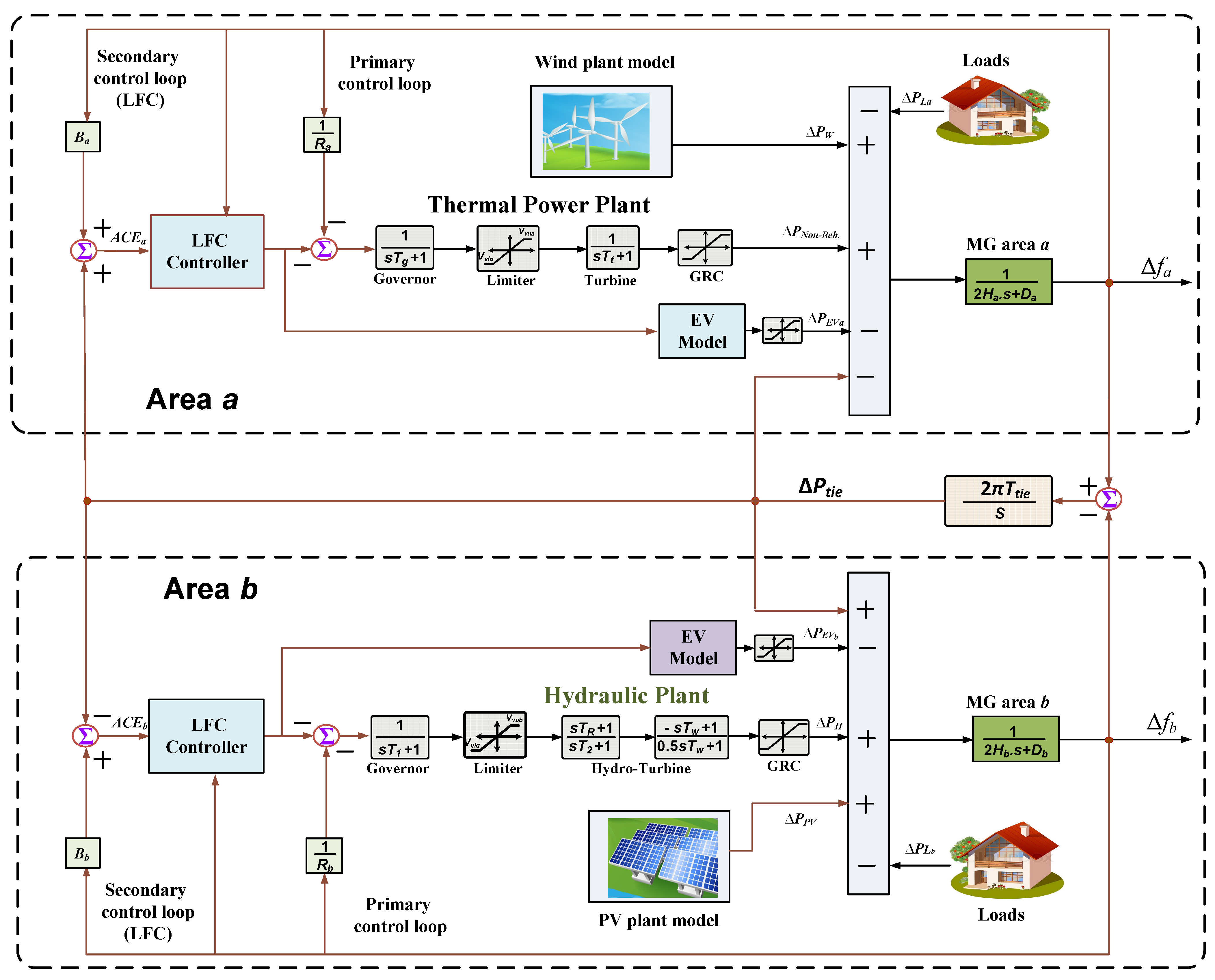
2. MG Model and Description

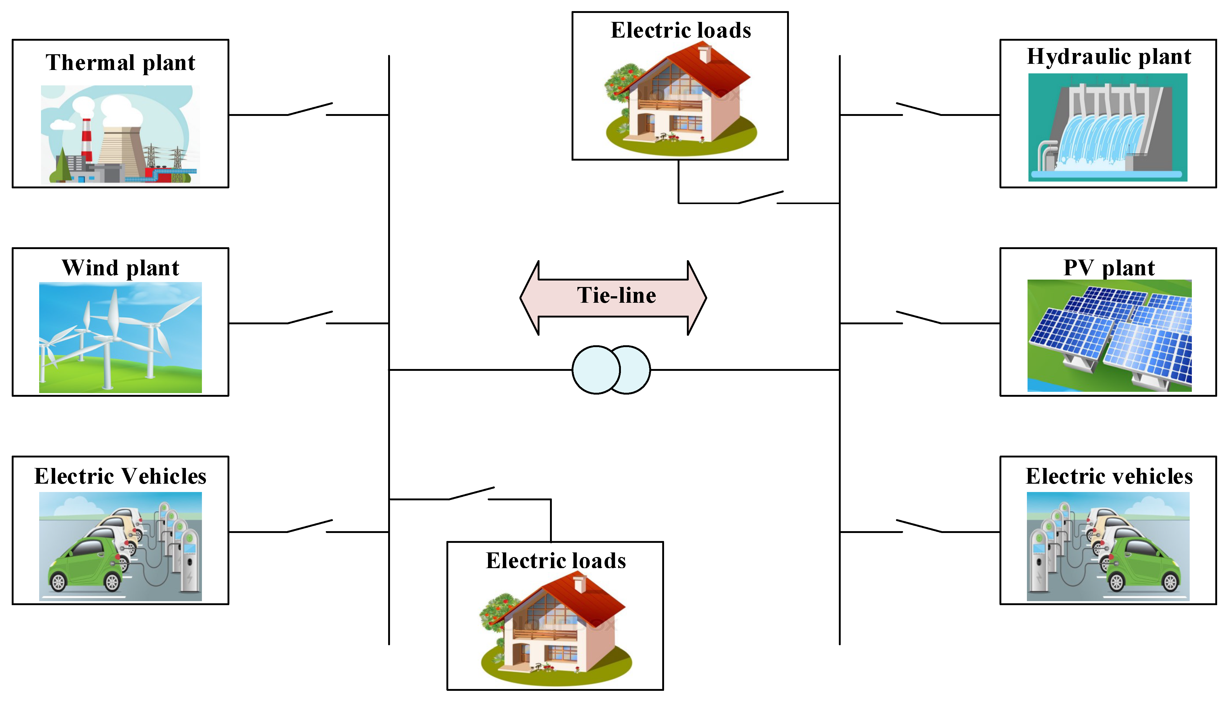
2.1. MGs’ Construction

Figure 1 shows the basic MG structure with the interconnection lines. The proposed 1+TD/FOTIDF control scheme is used in each area for controlling both existing generations and EV battery systems. It compensates for the power imbalance, which is reflected as deviations in system frequency and inter-areas tie-line power. In the studied MGs, RESs are distributed among interconnected areas considering wind generation in the first area (area a) and PV generation in the other area (Area b). The EVs are actively used through their inherent BESSs to participate during the frequency regulation process. The EVs are assumed to be equally divided between areas a and b. Additionally, conventional generation units are used in studied MGs by considering thermal plant units in area a and hydraulic plant units in area b. A MATLAB/SIMULINK jointed with an m-file is used for simulating the MGs with the proposed LFC. Complete MG element models are included in a single diagram as shown in Figure 2. Descriptions of various models are detailed in the following sub-sections.

2.2. Modeling of Thermal and Hydraulic Generators

The model transfer function (TF) for thermal plant units is usually represented by the governor stage $G_g\left(s\right)$, and turbine stage $G_t\left(s\right)$ considering the nonlinearity of generation rate constraints (GRC) which is given as 0.3 pu MW/min for thermal and hydraulic power plants. The implemented TFs for $G_t\left(s\right)$, and $G_g\left(s\right)$ are represented as [54]:

$$G_g\left(s\right)=\frac{1}{T_{g}s+1}$$

(1)

$$G_t\left(s\right)=\frac{1}{T_{t}s+1}$$

(2)

This leads to having the complete thermal plants model TF $G_T\left(s\right)$ as follows [55]:

$$G_T\left(s\right)=\frac{1}{T_{g}s+1}.\frac{1}{T_{t}s+1}$$

(3)

The performance of the hydraulic turbines relies on the value of inertia, water’s compressibility, and the pipes’ wall elasticity. By 1977, the IEEE committee had recommended hydraulic turbines’ mathematical modeling by assuming that the water flowing through penstock pipes is a non-compressible fluid and the water’s velocity is proportionally dependent on the gate valve. The water’s velocity in penstock pipes is represented as follows:

$$U=K_u.G.\sqrt{H_g}\frac{1}{T_{t}s+1}$$

(4)

where U, $H_g$, and G are the proportionality constant, the hydraulic head, and the gate valve’s position, respectively. The mechanical power from turbine $P_m$ is represented as:

$$P_m=K_p.H_g.U$$

(5)

The required time for water to travel over L length of conduit with velocity $U_0$ and gravity acceleration $a_g$ is expressed as;

$$T_w=\frac{L{U}_0}{a_g{H}_0}$$

(6)

Normally, hydraulic plants’ TFs are modeled using the governor TF $G_{gh}\left(s\right)$, droop compensation TF $G_{gh}\left(s\right)$, and penstock turbines TF $G_{th}\left(s\right)$. The complete hydraulic TF $G_h\left(s\right)$ is represented as [56]:

$$G_h\left(s\right)=\frac{1}{T_{1}s+1}.\frac{T_{R}s+1}{T_{2}s+1}.\frac{-T_{w}s+1}{0.5T_{w}s+1}$$

(7)

The MGs’ power system is usually modeled using first-order TF $G_{px}\left(s\right)$ as [56]:

$$G_{px}\left(s\right)=\frac{1}{2H_{x}s+D_x}$$

(8)

where $H_x$ stands for areas inertia constants and $D_x$ stands for areas damping constants.

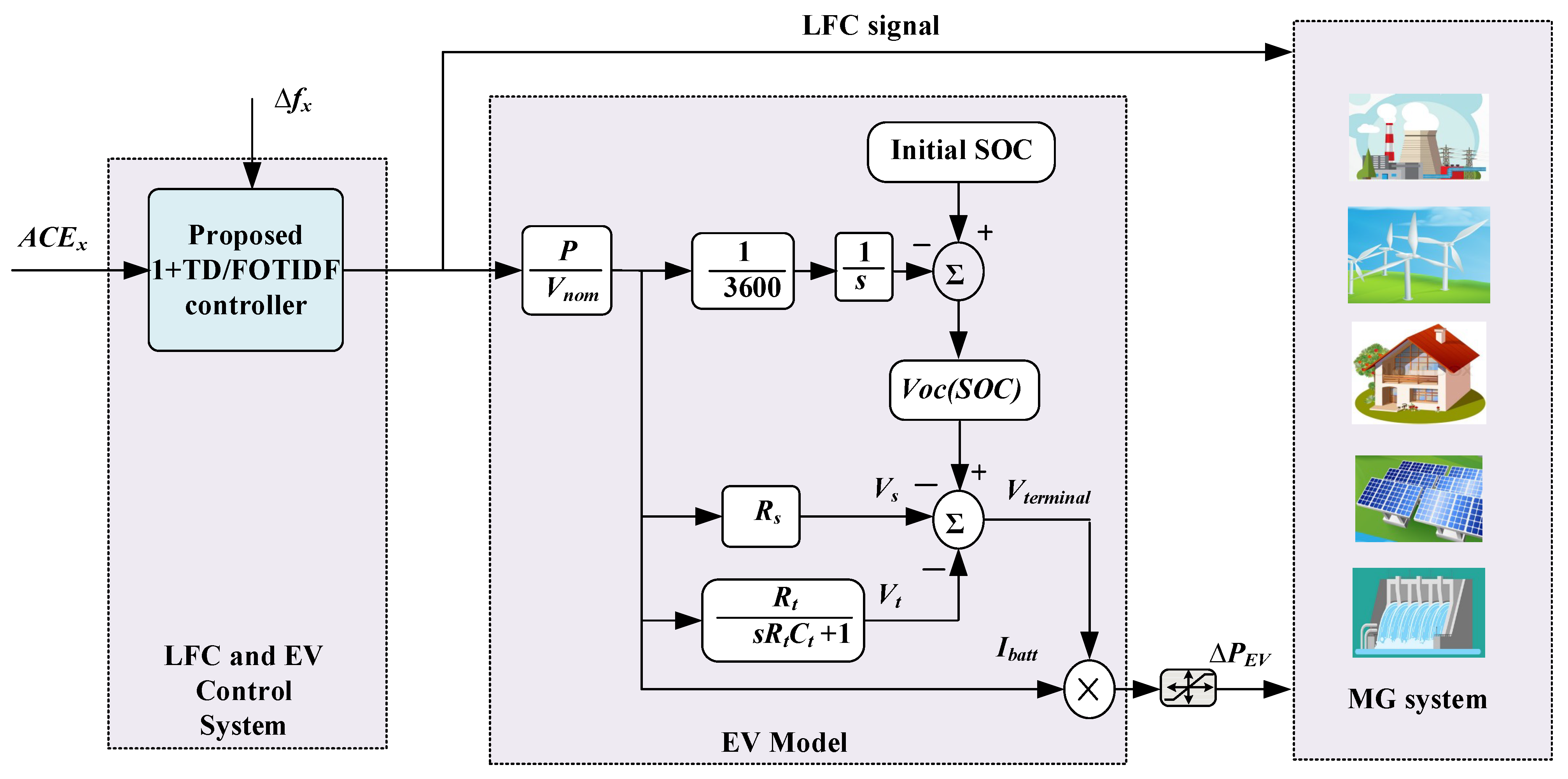
2.3. Modeling EVs’ BESSs

Figure 3 presents the implemented EV BESSs model. The proposed 1+TD/FOTIDF controller is employed in a centralized way in each area to control the existing generation units and the EV BESSs. The model contains a parallel RC branch using ($R_t$ and $C_t$). The RC branch describes the various transient overvoltages of the EVs BESS. The resistance $R_s$ is referred to as BESS thermal resistance. The regulation signal output from the regulation controller is transferred to the current to charge/discharge BESS using the $P/V_{nom}$ term while considering the initial state of charge (SOC) in the model. With the recent concerns of replacing traditional transportation systems with EVs in various applications, the use of their BESSs can be used for the charge/discharge process based on grid conditions. Their participation can be leveraged to reduce the necessity for additional ESSs in MGs. The outputted $V_{oc}$ of the EV model is related to the SOC of batteries (referred to $V_{oc}\left(SOC\right)$) based on the Nernst equation as follows [56]:

$$V_{oc}\left(SOC\right)=V_{nom}+S\frac{RT}{F}ln\left(\frac{SOC}{C_{nom}-SOC}\right)$$

(9)

where $V_{nom}$ is BESS’s nominal voltage, $C_{nom}$ is BESS’s nominal capacity (Ah). The sensitivity parameter S between $V_{oc}$ and BESS’s $SOC$. The gas constant is dented by R, the Faraday constant is represented by F, and temperature is represented by T.

2.4. Wind Plant’s Model

Outputted wind power possesses intermittency due to its dependency on environmental conditions, such as wind speed, ambient temperature conditions, etc. The continuous variation in wind speed during the day affects the power output from wind plants. The mechanical power taken from wind ($P_{WT}$) is represented by [57]:

$$P_{WT}=\frac{1}{2}\rho A_T{V}_W^3{C}_p(\lambda ,\beta )$$

(10)

where, $A_T$ blades swept area (in ${\mathrm{m}}^2$, $\rho$ stands for air density (in kg/${\mathrm{m}}^2$, $V_W$ is wind speed (in m/s), and $C_p(\lambda ,\beta )$ refers to power coefficient in function of tip-speed ratio $\lambda$ and pitch angle of blades $\beta$. It provides an indication of how much power is extracted from the wind by the turbine. The $C_p(\lambda ,\beta )$ is expressed as [57]:

$$C_p(\lambda ,\beta )=0.5({\lambda }_i-0.022{\beta }^2-5.6)e^{-0.17{\lambda }_i}$$

(11)

whereas, ${\lambda }_i$ and $\lambda$ are expressed as [57]:

$${\lambda }_i=\frac{3600\times R}{1609\times R}$$

(12)

$$\lambda =\frac{{\omega }_B\times R}{V_W}$$

(13)

The continuously varying wind power is represented in this paper to count for wind power uncertainty. The outputted power from the model is then passed by the model of the inverter system as a first-order TF. The implemented TF of the wind plant $G_{WT}\left(s\right)$ is represented by [54]:

$$G_{WT}\left(s\right)=\frac{K_{WT}}{T_{WT}s+1}$$

(14)

where $K_{WT}$ is the gain symbol of the wind plant and $T_{WT}$ is its associated time constant.

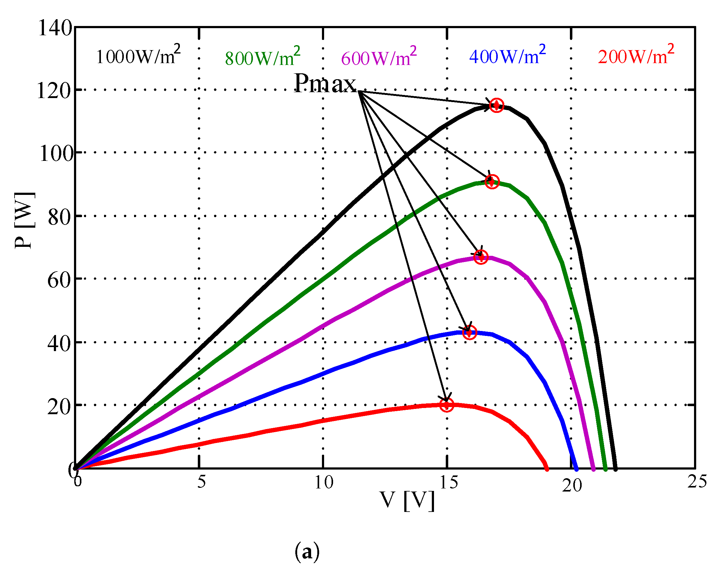
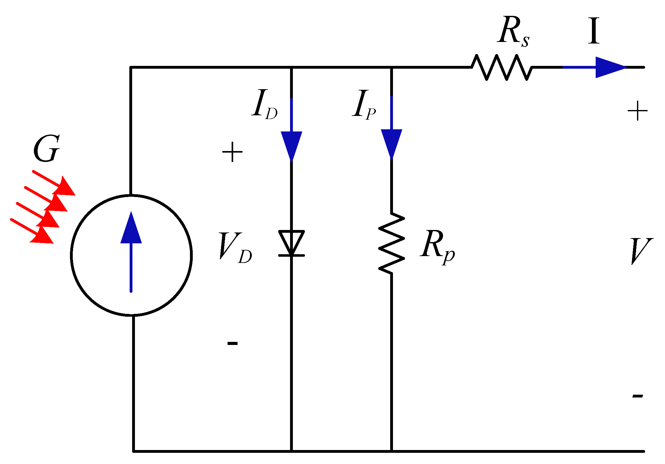
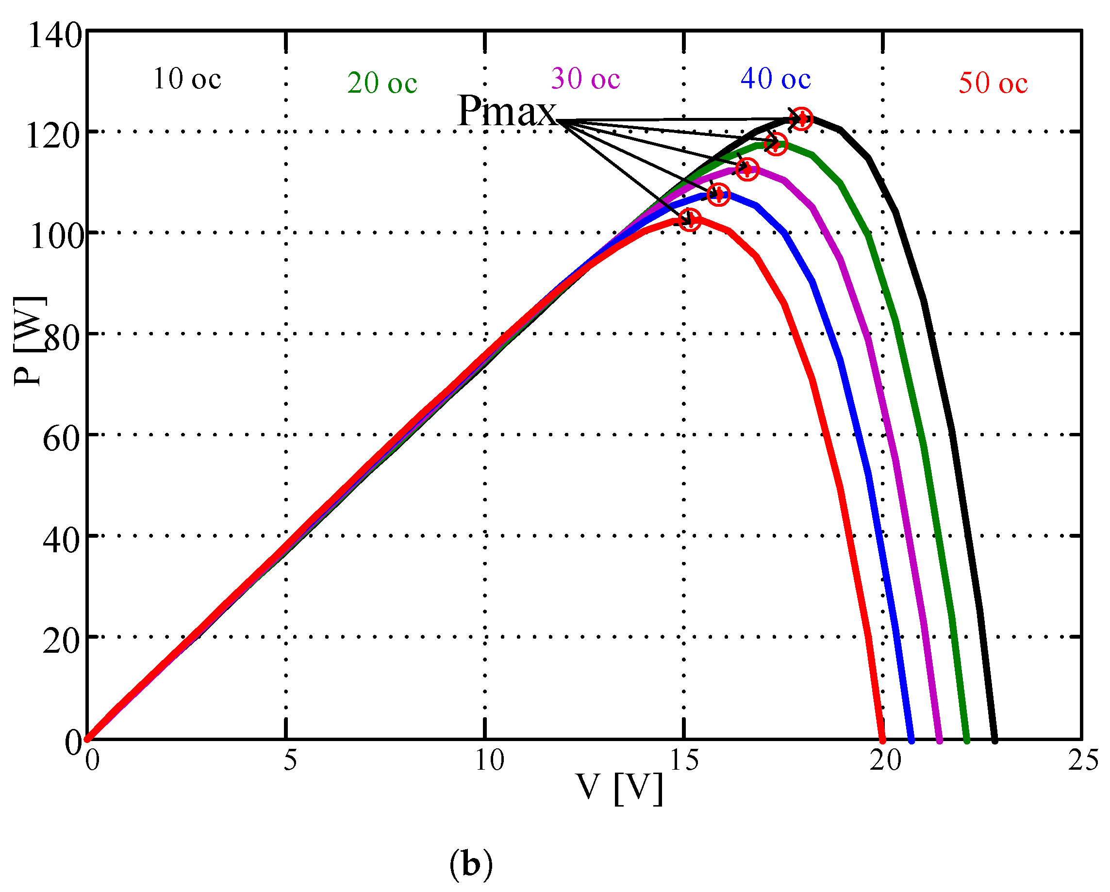
2.5. Modeling of PV Power Plants

A type of solar energy, known as solar PV, is one that uses the photo-electric effect to convert solar radiation into electrical power. Solar energy is coming from the sun and spread out into the space in the form of photons. When the photons strike the solar cells that connect the PV module, they transfer energy to the module, allowing negatively charged electrons to break free from their atoms. After absorbing photon energy, these electrons have enough energy to travel and head toward the opposite (negative) side of the panel, which is how the potential difference and electrical energy are produced.

The PV cell model seen in Figure 4 is employed to simulate the PV module. The open-circuit voltage ($V_{oc}$) and short-circuit current ($I_{sc}$) are determined under various weather conditions. The $I_{sc}$ and the $V_{oc}$ at standard weather conditions ($G_{st}$ = 1000 W/${\mathrm{m}}^2$ and $T_{st}$ = 25 °C) can be obtained from the PV module’s nameplate. The generated current by the incident light ($I_{PV}$), which is called short-circuit current ($I_{sc}$), is determined at a given cell temperature ($T_a$) as follows [58,59]:

$$I_{PV}=I_{scn}(1+a(T_a-T_n))\frac{G}{G_n}$$

(15)

where $I_{scn}$ represents Short circuit current at normal circumstances (25 °C, 1000 W/${\mathrm{m}}^2$). $T_a$ is the given cell temperature (K). a is the temperature coefficient of $I_{sc}$ in percent change per degree temperature. $G_n$ is the nominal value of irradiance, which is normally 1000 W/${\mathrm{m}}^2$. As seen from Figure 4, the output current delivered to the load can be expressed as [58,59]:

$$I=I_{PV}-I_0\left(e^{\frac{q(V+I{R}_s)}{nK{T}_a}}-1\right)-\frac{V_D}{R_p}$$

(16)

where $V_D$ is the diode voltage. The reverse saturation current of diode ($I_{on}$) at the reference temperature ($T_n$) is given as [58,59]:

$$I_{on}=\frac{I_{scn}}{e^{\frac{q{V}_{ocn}}{nK{T}_n}}-1}$$

(17)

where $V_{ocn}$ is the open circuit voltage at normal conditions. The reverse saturation current ($I_o$) at Ta is given as [58]:

$$I_o=I_{on}{\left(\frac{T_a}{T_n}\right)}^{\frac{3}{n}}{e}^{\frac{-q{E}_g}{nK}(\frac{1}{T_a}-\frac{1}{T_n})}$$

(18)

The series resistance ($R_s$) of the PV module has a large impact on the slope of the I-V curve near $V_{oc}$. The output voltage of the PV cell is given as:

$$V=V_D-I{R}_s$$

(19)

The PV module No. BP3115 is used in this paper. The PV module parameters at standard conditions (1000 W/${\mathrm{m}}^2$, 25 °C) are listed in

Table 1. The employed PV Module Parameters in the study.

Parameter	Value
Maximum Power value ($P_{max}$)	115 W
Voltage at Maximum Power value ($V_{mp}$)	17.1 V
Current at Maximum Power value ($I_{mp}$)	6.7 A
Voltage value at Open-Circuit ($V_{oc}$)	21.8 V
Current value at Short -Circuit ($I_{sc}$)	7.5 A

. As seen in the previous equations, changing the ambient temperature and the irradiance level affects the performance of the PV module. To verify the output power ranges of the used PV module with changing weather conditions, the PV module model is simulated and tested under changes in solar radiation and changes in the PV cell temperature. The simulation results of the PV power versus PV voltage at different irradiance levels and cell temperatures are shown in Figure 5a,b, respectively. As can be noted in Figure 5a, when the solar radiation is increased from 200 W/${\mathrm{m}}^2$ to 1000 W/${\mathrm{m}}^2$ with 200 W/${\mathrm{m}}^2$ steps and at a constant cell temperature (25 °C), the maximum power point (MPP) is increased from approximately 20 W at 200 W/${\mathrm{m}}^2$ to 115 W at 1000 W/${\mathrm{m}}^2$, and the $V_{oc}$ is slightly increased too. Moreover, the simulation results of the PV power versus PV voltage under different temperatures, 10 °C to 50 °C with 10 °C steps with constant solar radiation (1000 W/${\mathrm{m}}^2$), are shown in Figure 5b. In these curves, the MPP is increased by reducing the cell temperature.

The inverter system of PV generation is also included in the model using the TF $G_{PV}\left(s\right)$ and it is modeled as [60]:

$$G_{PV}\left(s\right)=\frac{K_{PV}}{T_{PV}s+1}$$

(20)

where, $K_{PV}$ and $T_{PV}$ refer to the gain, and the time constant of the PV power plant inverter system, respectively.

2.6. MG’s Complete Model

The complete studied MG’s system is shown in Figure 2. The system can be linearized and jointly represented in a single-state space model. The state space model is generally expressed as:

$$\dot{x}=Ax+B_1\omega +B_{2}u$$

(21)

$$y=Cx$$

(22)

where x is the vector of state variables, y is the vector of output states, $\omega$ includes the disturbances vector, and u includes control variables. A, $B_1$, $B_2$, and C are the obtained system parameters’ matrices in the linear state-space representation of the two-area power system. The representations of x and $\omega$ are conducted as:

$$x={\left[\begin{array}{cccccccccc}\Delta f_a& \Delta P_{ga}& \Delta P_{ga1}& \Delta P_{WT}& \Delta f_b& \Delta P_{gb}& \Delta P_{gb1}& \Delta P_{gb2}& \Delta P_{PV}& \Delta P_{tie,ab}\end{array}\right]}^T$$

(23)

$$\omega ={\left[\begin{array}{cccc}\Delta P_{la}& P_{WT}& \Delta P_{lb}& P_{PV}\end{array}\right]}^T$$

(24)

Control variables u include output from each controller ($C_{out,a}$ and $C_{out,b}$) and EV side power demand/injection ($\Delta P_{EVa}$ and $\Delta P_{EVb}$) based on charge/discharge commands. The control variables u are expressed as:

$$u={\left[\begin{array}{cccc}{C}_{out,a}& \Delta P_{E{V}_a}& C_{out,b}& \Delta P_{E{V}_b}\end{array}\right]}^T$$

(25)

System component representations are included in the state-space model using the matrices (A, $B_1$, $B_2$, and C). Their representation of studied MG systems is as follows:

$$A=\left[\begin{array}{cccccccccc}-\frac{D_a}{2H_a}& \frac{1}{2H_a}& 0& \frac{1}{2H_a}& 0& 0& 0& 0& 0& -\frac{1}{2H_a}\\ 0& -\frac{1}{T_t}& \frac{1}{T_t}& 0& 0& 0& 0& 0& 0& 0\\ -\frac{1}{R_a{T}_g}& 0& -\frac{1}{T_g}& 0& 0& 0& 0& 0& 0& 0\\ 0& 0& 0& -\frac{1}{T_{WT}}& 0& 0& 0& 0& 0& 0\\ 0& 0& 0& 0& -\frac{D_b}{2H_b}& \frac{1}{2H_b}& 0& 0& \frac{1}{2H_b}& \frac{1}{2H_b}\\ 0& 0& 0& 0& \frac{2T_R}{R_b{T}_1{T}_2}& -\frac{2}{T_w}& \frac{2T_2+2T_w}{T_2{T}_w}& \frac{2T_R-2T_1}{T_1{T}_2}& 0& 0\\ 0& 0& 0& 0& -\frac{T_R}{R_b{T}_1{T}_2}& 0& -\frac{1}{T_2}& \frac{T_1-T_R}{T_1{T}_2}& 0& 0\\ 0& 0& 0& 0& -\frac{1}{R_b{T}_1}& 0& 0& -\frac{1}{T_1}& 0& 0\\ 0& 0& 0& 0& 0& 0& 0& 0& -\frac{1}{T_{PV}}& 0\\ 2\pi T_{\mathit{tie,eq}}& 0& 0& 0& -2\pi T_{\mathit{tie,eq}}& 0& 0& 0& 0& 0\end{array}\right]$$

(26)

$$B_1=\left[\begin{array}{cccc}-\frac{1}{2H_a}& 0& 0& 0\\ 0& 0& 0& 0\\ 0& 0& 0& 0\\ 0& \frac{K_{WT}}{T_{WT}}& 0& 0\\ 0& 0& -\frac{1}{2H_b}& 0\\ 0& 0& 0& 0\\ 0& 0& 0& 0\\ 0& 0& 0& 0\\ 0& 0& 0& \frac{K_{PV}}{T_{PV}}\\ 0& 0& 0& 0\end{array}\right],\text{ and }{B}_2=\left[\begin{array}{cccc}0& -\frac{1}{2H_a}& 0& 0\\ 0& 0& 0& 0\\ -\frac{1}{T_g}& 0& 0& 0\\ 0& 0& 0& 0\\ 0& 0& 0& -\frac{1}{2H_b}\\ 0& 0& \frac{2T_R}{T_1{T}_2}& 0\\ 0& 0& -\frac{T_R}{T_1{T}_2}& 0\\ 0& 0& -\frac{1}{T_1}& 0\\ 0& 0& 0& 0\\ 0& 0& 0& 0\end{array}\right]$$

(27)

$$C=\left[\begin{array}{cccccccccc}1& 0& 0& 0& 0& 0& 0& 0& 0& 0\\ B_a& 0& 0& 0& 0& 0& 0& 0& 0& 1\\ 0& 0& 0& 0& 1& 0& 0& 0& 0& 0\\ 0& 0& 0& 0& B_b& 0& 0& 0& 0& -1\end{array}\right]$$

(28)

The implemented models use the parameters presented in [54].

Table 2. Used Parameters for representing MGs system (with $x\in \{a,b\}$), [54].

Parameters	Symbols	Value
		Area $\mathit{a}$	Area $\mathit{b}$
Rated MGs’ capacity	$P_{rx}$ (MW)	1200	1200
Droops constant	$R_x$ (Hz/MW)	2.4	2.4
Frequency bias values	$B_x$ (MW/Hz)	0.4249	0.4249
Valve gate limiting value (minimum)	$V_{vlx}$ (p.u.MW)	−0.5	−0.5
Valve gate limiting value (maximum)	$V_{vux}$ (p.u.MW)	0.5	0.5
Time constant for thermal governor	$T_g$ (s)	0.08	-
Thermal turbines’ (time constant)	$T_t$ (s)	0.3	-
Governor of hydraulic generator (time constant)	$T_1$ (s)	-	41.6
Transient droops time constant for hydraulic governor	$T_2$ (s)	-	0.513
Governor of hydraulic generator resetting time	$T_R$ (s)	-	5
Hydraulic turbines’ water starting time	$T_w$ (s)	-	1
Inertia’s constants	$H_x$ (p.u.s)	0.0833	0.0833
Damping coefficient	$D_x$ (p.u./Hz)	0.00833	0.00833
PV generations time constant	$T_{PV}$ (s)	-	1.3
PV generations’ gains	$K_{PV}$ (s)	-	1
Wind generations’ time constants	$T_{WT}$ (s)	1.5	-
Wind generations’ gains	$K_{WT}$ (s)	1	-
EV BESSs’ models
Penetration level	-	10%	10%
BESS voltages (nominal)	$V_{nom}$ (V)	364.8	364.8
BESS capacity	$C_{nom}$ (Ah)	66.2	66.2
Series resistances	$R_s$ (ohms)	0.074	0.074
Transient resistance	$R_t$ (ohms)	0.047	0.047
Transient capacitances	$C_t$ (farad)	703.6	703.6
Constants value	$RT/F$	0.02612	0.02612
BESS’s SOC (maximum)	%	95	95
BESS’s energy capacity	$C_{batt}$ (kWh)	24.15	24.15

summarizes the employed parameters for the developed modeling of interconnected MG components.

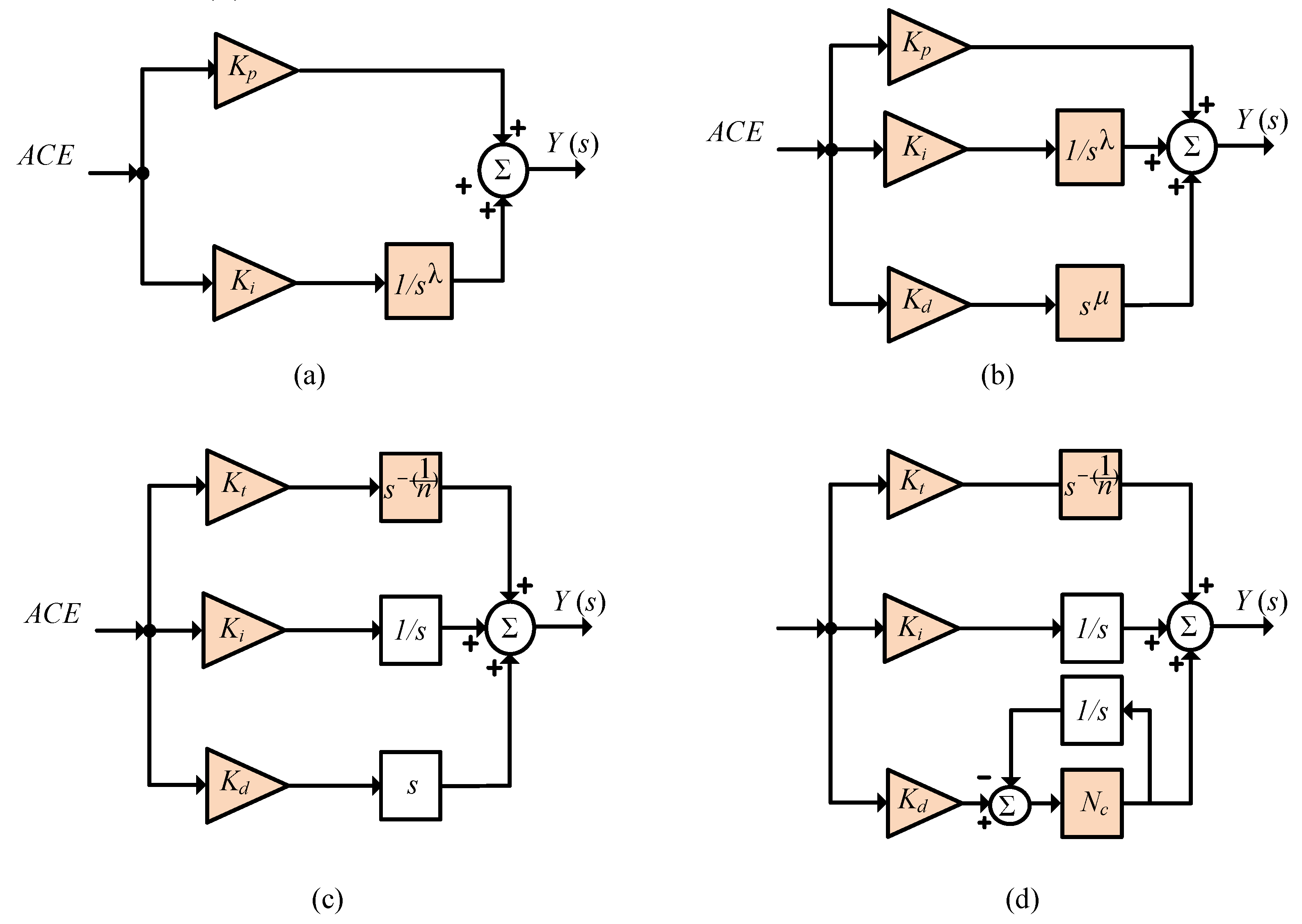
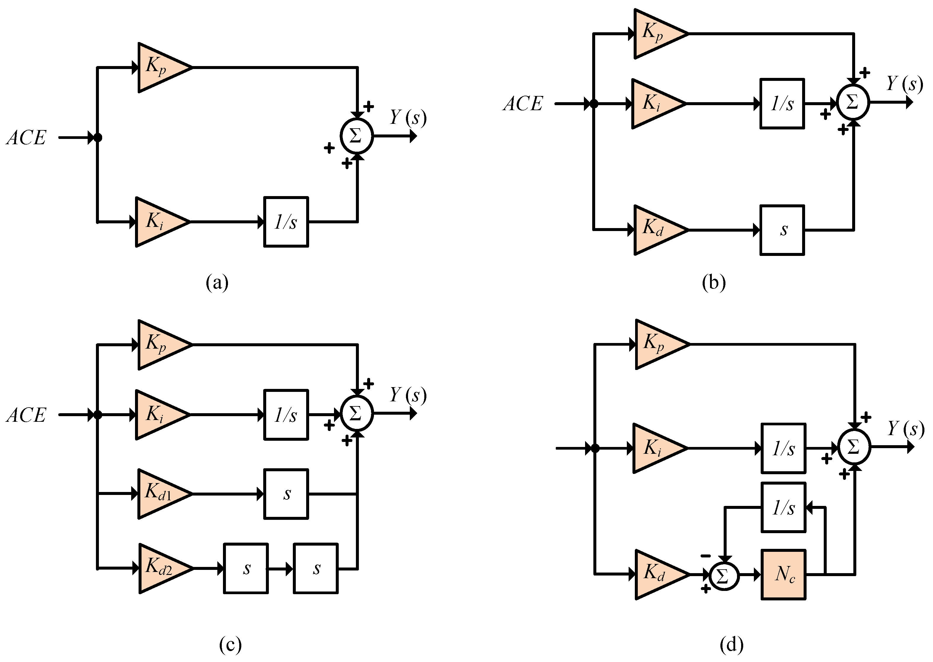
3. Overview of LFC and FO Operators

3.1. LFC Schemes in Literature

As explained in the literature review, numerous integer order (IO), fractional order (FO), and hybrid IO-FO LFCs have been proposed in the literature. In general, IO-based control schemes have found wide employment in several frequency regulation controllers. The I, PI, ID, PIDD, PID, and PIDF are examples of vastly applied IO LFC in literature. The TF representation $C\left(s\right)$ of these controllers are as follows [54,55,56,57]:

$$\begin{array}{c}{C}_{PI}\left(s\right)=\frac{Y\left(s\right)}{E\left(s\right)}=K_p+\frac{K_i}{s}\\ C_{PIDD}\left(s\right)=\frac{Y\left(s\right)}{E\left(s\right)}=K_p+\frac{K_i}{s}+K_{d1}s+K_{d2}{s}^2\\ C_{PID}\left(s\right)=\frac{Y\left(s\right)}{E\left(s\right)}=K_p+\frac{K_i}{s}+K_{d}s\\ C_{PIDF}\left(s\right)=\frac{Y\left(s\right)}{E\left(s\right)}=K_p+\frac{K_i}{s}+K_{d}s\frac{N_f}{s+N_f}\end{array}$$

(29)

For instance, $K_i$, $K_p$, and $K_d$ represent PID gains for integral, proportional, and derivative branches. They represent the flexibility of the PID LFC design process to optimize the MGs’ frequency regulation functionality. The PIDF possesses the filter gain as an additional design flexibility parameter. Figure 6 shows the representation of the most common IO LFC in literature.

On the other hand, FO-based LFC schemes have been presented to benefit from FO operators and their associated flexibility. The added FO integrator operator and FO derivative operator increase the DOF of LFC systems. Figure 7 shows some examples of existing FO LFC in literature. Some examples of existing FO LFC in literature are represented as [54,55,56,57]:

$$\begin{array}{c}{C}_{FOPI}\left(s\right)=\frac{Y\left(s\right)}{E\left(s\right)}=K_p+\frac{K_i}{s^{\lambda }}\\ C_{TID}\left(s\right)=\frac{Y\left(s\right)}{E\left(s\right)}=K_t{s}^{-\left(\frac{1}{n}\right)}+\frac{K_i}{s}+K_{d}s\\ C_{FOPID}\left(s\right)=\frac{Y\left(s\right)}{E\left(s\right)}=K_p+\frac{K_i}{s^{\lambda }}+K_d{s}^{\mu }\\ C_{TIDF}\left(s\right)=\frac{Y\left(s\right)}{E\left(s\right)}=K_t{s}^{-\left(\frac{1}{n}\right)}+\frac{K_i}{s}+K_{d}s\frac{N_f}{s+N_f}\end{array}$$

(30)

From Equation (30), the FO-based LFC includes the added FO operators ($\lambda$ for integrator, and $\mu$ for derivative) to the gains ($K_p$, $K_t$, $K_i$, and $K_d$), which is reflected as more freedom in optimizing MG frequency regulation response. The FO operators in Equation (30) are usually tuned in the range of [0, 1].

3.2. FO Operators Representation

An important issue of FO control is the way to implement and represent FO operators using available digital control platforms. There are several definitions for FO calculus, such as the Caputo definition, the Grunwald–Letnikov definition, and the Riemann–Liouville definition [61]. In the definition of Grunwald–Letnikov, ${\alpha }_{th}$ is used as a fractional derivative to function f inside a to t limits. It is represented as [62]:

$$D^{\alpha }{|}_a^t=\underset{h\to 0}{lim}\frac{1}{h^{\alpha }}\sum _{r=0}^{\frac{t-a}{h}}{(-1)}^r\left(\begin{array}{c}n\\ r\end{array}\right)f(t-rh)$$

(31)

In which, h is referred to as step time and $[·]$ in integer terms’ operator for the Grunwald–Letnikov definition. In (36), n lies in the range ($n-1$$<\alpha <n$). Also, binomial coefficients can be expressed as [62]:

$$\left(\begin{array}{c}n\\ r\end{array}\right)=\frac{\mathsf{\Gamma }(n+1)}{\mathsf{\Gamma }(r+1)\mathsf{\Gamma }{(n-r+1)}^{\prime }}$$

(32)

where the function of gamma in (32) is normally defined as [61]:

$$\mathsf{\Gamma }(n+1)={\int }_0^{\infty }{t}^{x-1}{e}^{-t}dt$$

(33)

The definition of Riemann–Liouville avoids the sum and limits. It employs the integer-based derivative and integral terms as [63]:

$$D^{\alpha }{|}_a^t=\frac{1}{\mathsf{\Gamma }(n-\alpha )}(\frac{d}{dt}{)}^n{\int }_a^t\frac{f\left(\tau \right)}{{(t-\tau )}^{\alpha -n+1}}d\tau$$

(34)

The definition of Caputo is represented as [62]:

$$D^{\alpha }{|}_a^t=\frac{1}{\mathsf{\Gamma }(n-\alpha )}{\int }_a^t\frac{f^{\left(n\right)}\left(\tau \right)}{{(t-\tau )}^{\alpha -n+1}}d\tau$$

(35)

Additionally, general FO operators are through employing $D^{\alpha }{|}_a^t$ as follows:

$$D^{\alpha }{|}_a^t=\left\{\begin{array}{cc}\alpha >0\to \frac{{\mathrm{d}}^{\alpha }}{\mathrm{d}{t}^{\alpha }}\hfill & \mathrm{FO}\mathrm{derivative}\hfill \\ \alpha <0\to {\int }_{t_0}^{t_{\mathrm{f}}}\mathrm{d}{t}^{\alpha }\hfill & \mathrm{FO}\mathrm{integral}\hfill \\ \alpha =0\to 1\hfill \end{array}\right.$$

(36)

For the proper implementation using digital control processors, Oustaloup recursive approximation (ORA) has verified superior performance for implementing FO operators using digital processors [61]. The ORA representation is employed in this work for implementing FO controllers. The ${\alpha }^{th}$ FO based derivative ($s^{\alpha }$) is mathematically-approximated as [61]:

$$s^{\alpha }\approx {\omega }_h^{\alpha }\prod _{k=-N}^N\frac{s+{\omega }_k^z}{s+{\omega }_k^p}$$

(37)

where ${\omega }_k^p$ and ${\omega }_k^z$ refer to the locations of poles, and zeros, respectively, for the ${\omega }_h$ sequence. The calculations are performed as follows:

$${\omega }_k^z={\omega }_b{\left(\frac{{\omega }_h}{{\omega }_b}\right)}^{\frac{k+N+\frac{1-\alpha }{2}}{2N+1}}$$

(38)

$${\omega }_k^p={\omega }_b{\left(\frac{{\omega }_h}{{\omega }_b}\right)}^{\frac{k+N+\frac{1+\alpha }{2}}{2N+1}}$$

(39)

$${\omega }_h^{\alpha }={\left(\frac{{\omega }_h}{{\omega }_b}\right)}^{\frac{-\alpha }{2}}\prod _{k=-N}^N\frac{{\omega }_k^p}{{\omega }_k^z}$$

(40)

The existing poles/zeros number for the approximated FO ORA representation is $(2N+1)$, and N defines the ORA order. The utilized ORA representation in this work is performed using $(M=5)$ within ($\omega \in [{\omega }_b,{\omega }_h]$) between $[{10}^{-3},{10}^3]$ rad/s frequency limits.

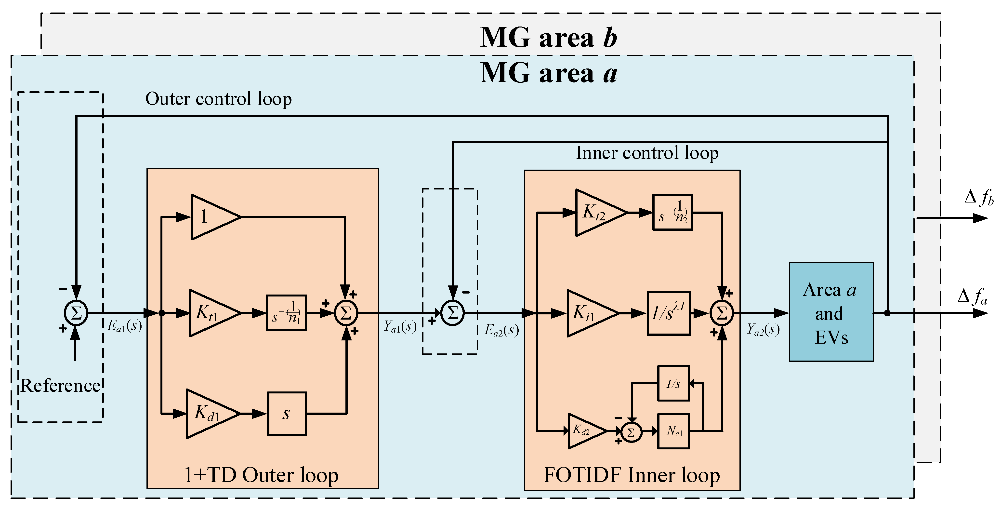
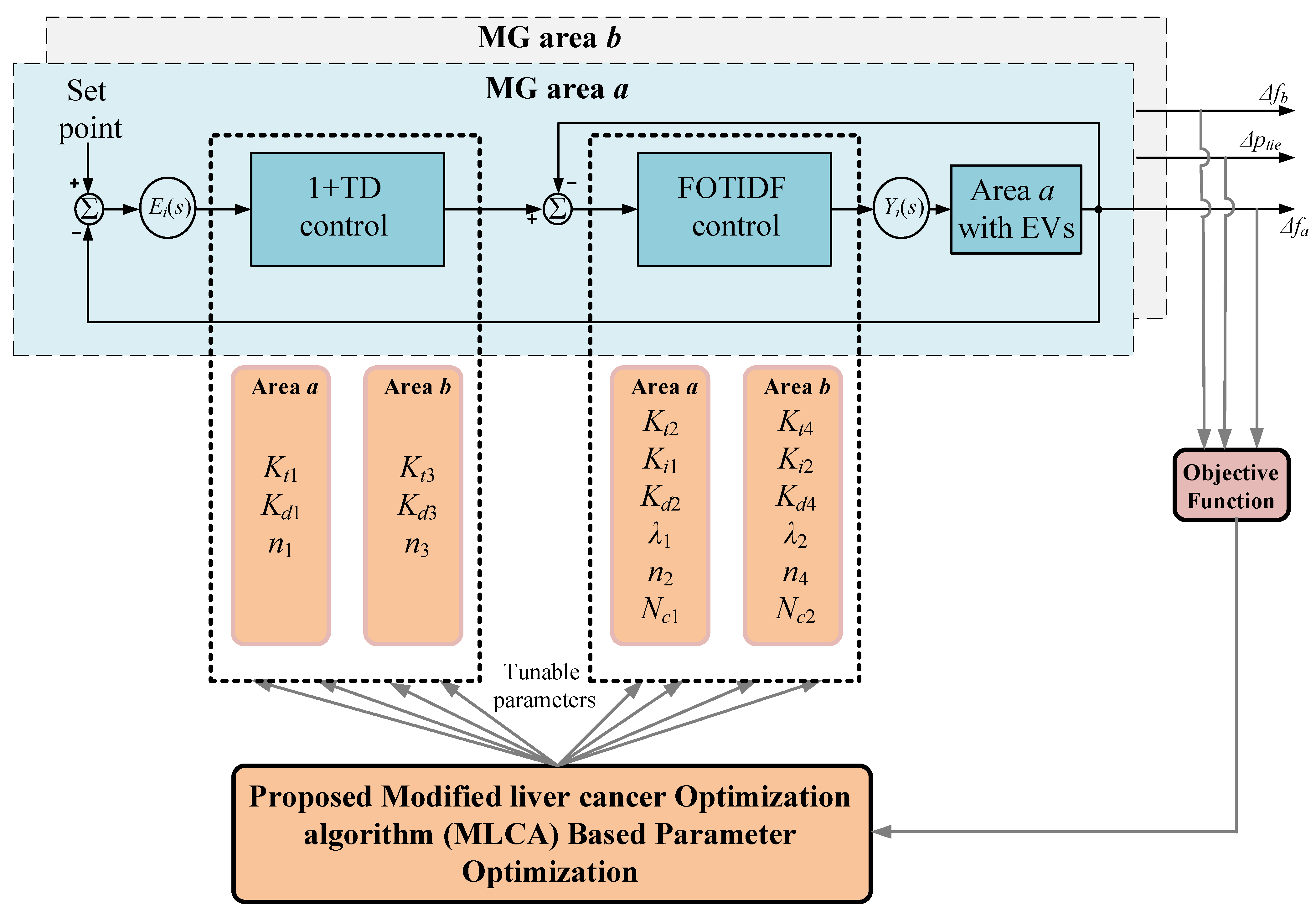
3.3. Proposed 1+TD/FOTIDF LFC

From the above-mentioned discussion about existing LFC in the literature, and the associated extra flexibility of using FO operators, this paper proposed a hybrid IO with the FO-based LFC method. The conventional IO and FO structures use the ACE feedback signal as an input for the controller. This leads to a slower response in these LFC schemes. Moreover, their ability to mitigate existing disturbances due to load and/or generation changes is poor. The proposed controller is based on the cascaded LFC methods. It uses two cascaded LFC loops in its structure. The 1+TD is used in implementing the outer controller loop by using the ACE signal as a feedback signal to this stage. The second loop uses the frequency deviation in each area as a feedback signal employing the FOTIDF in this loop. Therefore, the proposed LFC control is based on a 1+TD/FOTIDF controller with two feedback signals in each area (ACE and $\Delta f_x$). Figure 8 presents the proposed 1+TD/FOTIDF controller for interconnected MGs.

It can be seen that the proposed 1+TD/FOTIDF combines the benefits of IO with FO control systems. Adding 1 to the TD controller and cascading it with the FOTIDF controller leads to reducing the control complexity and facilitating the parameter determination compared with using the proportional term as proven in [64,65]. Additionally, it uses two different inner signals to the outer and inner control loops ($AC{E}_a$ and $\Delta f_a$ in area a) and ($AC{E}_b$ and $\Delta f_b$ in area b). The use of $AC{E}_a$ and $AC{E}_b$ in outer loops enables the proposed LFC method to mitigate the low-frequency disturbances in the systems. The use of $\Delta f_a$ and $\Delta f_b$ in inner loops enables the mitigation of existing high-frequency disturbances in MG systems. Therefore, improved disturbance rejection capability is obtained through proposed cascaded 1+TD/FOTIDF loops.

The input to the outer loop is ACE signals of each area ($\left(AC{E}_a\right)$, and $\left(AC{E}_b\right)$), which are expressed as error signals for the outer loop as $E_{a1}\left(s\right)$ and $E_{b1}\left(s\right)$, respectively, in this stage. These inputs are represented as:

$$\begin{array}{c}{E}_{a1}\left(s\right)=AC{E}_a=\Delta P_{tie}+B_a\Delta f_a\\ E_{b1}\left(s\right)=AC{E}_b=A_{ab}\Delta P_{tie}+B_b\Delta f_b\end{array}$$

(41)

where $\left(A_{ab}\right)$ refers to the capacity ratio among MGs areas a and b. The outputted control signals from this stage are $Y_{a1}\left(s\right)$ and $Y_{b1}\left(s\right)$. The representation of this outer loop is made as follows:

$$\begin{array}{c}{Y}_{a1}\left(s\right)=[1+K_{t1}{s}^{-\left(\frac{1}{n_1}\right)}+K_{d1}s].E_{a1}\left(s\right)\\ Y_{b1}\left(s\right)=[1+K_{t3}{s}^{-\left(\frac{1}{n_3}\right)}+K_{d3}s].E_{b1}\left(s\right)\end{array}$$

(42)

From Equation (48), each MG outer loop has three tunable control parameters, which gives six total tunable parameters in the studied two areas. In MG area a, the three tunable control parameters are ($K_{t1}$, $K_{d1}$, and $n_1$) inside the 1+TD controller loop. For MG area b, the tunable parameters are ($K_{t3}$, $K_{d3}$, and $n_3$).

The output of the first outer loop is fed with frequency deviation signals ($\Delta f_a$, and $\Delta f_b$) to the outer control stage. The error of the inputted signals $E_{a2}\left(s\right)$ and $E_{b2}\left(s\right)$ for second inner loop are represented as:

$$E_{a2}\left(s\right)=Y_{a1}\left(s\right)-\Delta f_a{E}_{b2}\left(s\right)=Y_{b1}\left(s\right)-\Delta f_b$$

(43)

In the inner loop, the FOTIDF is utilized in this stage. The control output ($Y_{a2}\left(s\right)$ and $Y_{b2}\left(s\right)$) is expressed as:

$$\begin{array}{c}{Y}_{a2}\left(s\right)=[1+K_{t2}{s}^{-\left(\frac{1}{n_2}\right)}+\frac{K_{i1}}{s^{{\lambda }_1}}+K_{d2}\frac{N_{c1}}{s+N_{c1}}].E_{a2}\left(s\right)\\ Y_{b2}\left(s\right)=[1+K_{t4}{s}^{-\left(\frac{1}{n_4}\right)}+\frac{K_{i2}}{s^{{\lambda }_2}}+K_{d4}\frac{N_{c2}}{s+N_{c2}}].E_{b2}\left(s\right)\end{array}$$

(44)

From Equation (50), the MG area a has six tunable parameters ($K_{t2}$, $n_2$, $K_{i1}$, ${\lambda }_1$, $K_{d2}$, and $N_{c2}$) for designing its inner controller. MG area b has ($K_{t4}$, $n_4$, $K_{i2}$, ${\lambda }_2$, $K_{d4}$, and $N_{c2}$) tunable design parameters. There are a total of 12 tunable design parameters in the inner stage. Accordingly, the total representation of the proposed 1+TD/FOTIDF controller can be expressed as:

$$\begin{array}{c}{Y}_{a2}\left(s\right)=[(1+K_{t1}{s}^{-\left(\frac{1}{n_1}\right)}+K_{d1}s)AC{E}_a-\Delta f_a].[1+K_{t2}{s}^{-\left(\frac{1}{n_2}\right)}+\frac{K_{i1}}{s^{{\lambda }_1}}+K_{d2}\frac{N_{c1}}{s+N_{c1}}]\end{array}$$

(45)

$$\begin{array}{c}{Y}_{b2}\left(s\right)=[(1+K_{t3}{s}^{-\left(\frac{1}{n_3}\right)}+K_{d3}s)AC{E}_b-\Delta f_b].[1+K_{t4}{s}^{-\left(\frac{1}{n_4}\right)}+\frac{K_{i2}}{s^{{\lambda }_2}}+K_{d4}\frac{N_{c2}}{s+N_{c2}}]\end{array}$$

(46)

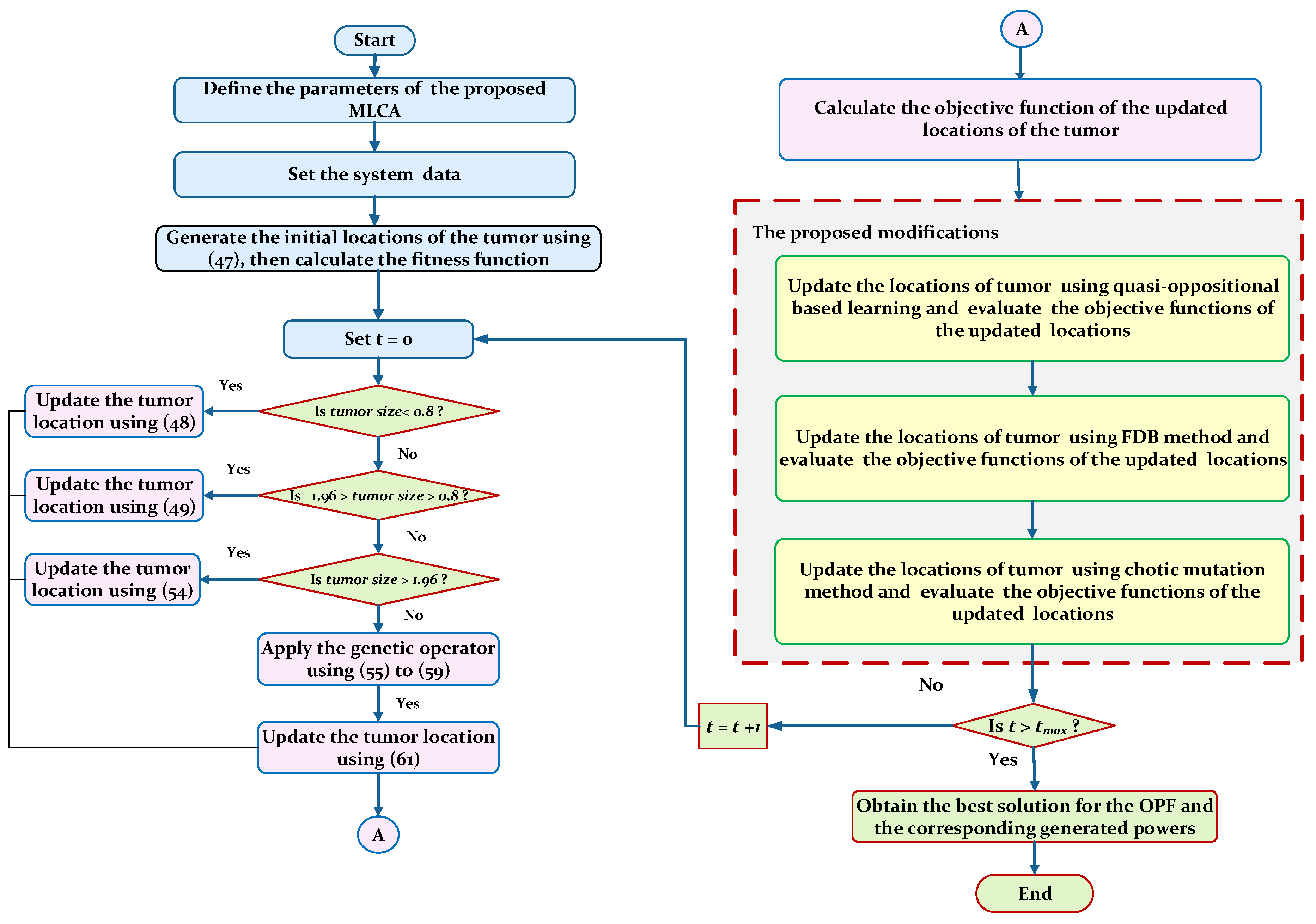
4. The Proposed Modified Liver Cancer Optimization Algorithm and Its Performance Verification

4.1. Liver Cancer Optimization Algorithm

The liver cancer optimization algorithm (LCA) is a developed optimizer that simulates liver tumor takeover and growth progression [66]. The LCA consists of several stages which are conceptualized from liver tumors and these stages can be defined as follows:

4.1.1. Tumor Size Estimation

It is important to calculate the size of the tumor for the following stages. For assigning the size of the tumor, it is assumed that the tumor has a hemi-ellipsoid shape, length, width and height. The initial tumor volume (location) can be calculated based on random opposition-based learning (ROBL) as follows:

$$\begin{array}{c}{X}_i^{0j}=\frac{\pi }{6}\left(L{e}^j\right).\left(W{i}^j\right).\left(H{i}^j\right)-(Ib+(ub-Ib)-r_d\times X_i^j)\end{array}$$

(47)

where $X_i^{0j}$ is a vector that is opposite to $X_i^j$. $lb$ and $ub$ represent the lower and the upper boundaries of variables. $Le$, $Wi$ and $Hi$ represent the length, the width and the height of the tumor, respectively. $r_d$ represents a random value within [0, 1]. The height and width represent random factors in the range [0–1]. The increase in the tumor volume can be described as follows:

$${X=\frac{\pi }{6}.f.(Le.Wi)}^{3/2}$$

(48)

where f is the constant value that equals 1.

4.1.2. Tumor Replication

This stage is considered a dangerous stage of the tumor and is manipulated in many places in the liver where hepatocellular carcinoma increases exponentially. The volume or the location of the tumor in this stage can be assigned as follows:

$$p^i=\frac{dV}{dt}=r\times X\in [1...T]\mathrm{and}i\in [1...N]$$

(49)

where P refers to the tumor growth location. T denotes the maximum iteration number while N refers to the population numbers. The spread of the tumor in the liver can be found by the levy flight mechanism as follows:

$$\upsilon \left(D\right)=0.01\times \frac{rand(1,D)\times \sigma }{{\left|rand(1,D)\right|}^{\frac{1}{\beta }}}$$

(50)

$$={\left(\frac{\mathsf{\Gamma }(1+\beta )\times sin\left(\frac{\pi \beta }{2}\right)}{\mathsf{\Gamma }\left(\frac{1+\beta }{2}\right)\times \beta \times 2\left(\frac{\beta -1}{2}\right)}\right)}^{\frac{1}{\beta }}$$

(51)

In this stage, LCA used the tumor-spreading mechanism and picked the best portion of the liver to assess its situation and determine the next procedure. This action can be mathematically represented as follows:

$$y=X+P$$

(52)

$$Z=Y+S\times LF\left(D\right)$$

(53)

$$X_{t+1}^i=\left\{\begin{array}{cc}y\hfill & \mathrm{if}fit\left(y\right)<fit{X}_t^i)\hfill \\ z\hfill & \mathrm{if}fit\left(z\right)<fit{X}_t^i)\hfill \end{array}\right.$$

(54)

where D represents the dimensions of the problem. S is a random vector in [0–1]. $fit$ refers to the fitness function.

4.1.3. Tumor Spreading

This stage is conceptualized by the spreading of the tumor to other body organs. Two operators are used to describe the spreading of the tumor including the mutation and the crossover. In the mutation operator, the populations will update their locations based on the mutation rate ($ϵ$), in which two vectors y and z were used to update the locations of the old vector if its random values are less than the mutation rate. The mutation process of the LCA can be described as follows:

$$y_{Mut}=\left\{\begin{array}{cc}X\hfill & \mathrm{if}{r}_1\ge ϵ\hfill \\ y\hfill & else\hfill \end{array}\right.$$

(55)

$$y_{Mut}=\left\{\begin{array}{cc}X\hfill & \mathrm{if}{r}_2\ge ϵ\hfill \\ z\hfill & else\hfill \end{array}\right.$$

(56)

In which,

$$ϵ=\frac{t}{T};$$

(57)

$$y=|X-X_i^j|$$

(58)

$$z=y-S$$

(59)

where, S has D elements captured from random values within [0, 1]. In the crossover, a new vector is generated by a combination of two individuals as described in the following equations:

$$X_{Croos}=\tau \times y_{Mut}+(1-{\tau }^{\prime })\times Z_{Mut},\tau \ne {\tau }^{\prime }$$

(60)

where ${\tau }^{\prime }$ and $\tau$ are random vectors. The locations of the newly updated tumors will be updated based on the fitness function values as follows:

$$X_{t+1}^i=\left\{\begin{array}{cc}{y}_{Mut}\hfill & \mathrm{if}fit\left(y_{Mut}\right)<fit\left(X^i\right)\hfill \\ z_{Mut}\hfill & \mathrm{if}fit\left(z_{Mut}\right)<fit\left(X^i\right)\hfill \\ X_{Cross}\hfill & \mathrm{if}fit\left(W_{cross}\right)<fit\left(X^i\right)\hfill \end{array}\right.$$

(61)

4.2. The Proposed Modified Liver Cancer Algorithm

The proposed MLCA is based on enhancing the performance of the standard LCA using three modifications including the fitness distance balance (FDB), and the quasi-oppositional based learning (QOBL).

4.2.1. The FDB Method

The FDB is an efficient selection strategy that was applied to numerous optimization methods for performance improvement [67,68,69,70,71,72]. The FDB is based on updating the current populations based on the distance that was determined between the best solution and the current candidates as well as its fitness value. The corresponding distance of the FDB can be expressed as follows:

$$Di{s}_i=\sqrt{{(X_i^1-X_{best,1})}^2+{(X_i^2-X_{best,2})}^2+\cdots +{(X_i^d-X_{best,d})}^2}$$

(62)

where $X_{best1}$ is the best solution while $X_i^j$ is the current solution. The distance and the fitness function values are represented as vectors as follows:

$$Obj=[Ob{j}_1,Ob{j}_2,\cdots ,Ob{j}_n]$$

(63)

$$Dis=[Di{s}_1,Di{s}_2,\cdots ,Di{s}_n,]$$

(64)

The next step in the FDB is to normalize the distance and the fitness as follows:

$$normDi{s}_i=\frac{Di{s}_i-Di{s}_{min}}{Di{s}_{max}-Di{s}_{min}}$$

(65)

$$normOb{j}_i=\frac{Ob{j}_i-Ob{j}_{min}}{Ob{j}_{max}-Ob{j}_{min}}$$

(66)

where $Di{s}_{min}$ and $Di{s}_{max}$ refer to the minimum and the maximum values of the distances, respectively. $Ob{j}_{min}$ and $Ob{j}_{max}$ refer to the minimum and maximum values of the objective functions. After the previous step, the score of each population will be calculated and also the score vector using Equations (67) to (69).

$$\rho =0.5\times \left(1+\frac{t}{t_{max}}\right)$$

(67)

$$Sco{r}_i=\rho \times (1-\mathrm{norm}Ob{j}_i)+(1-\rho )\times (1-\mathrm{norm}Di{s}_i)$$

(68)

$$Scor=[Sco{r}_1,Sco{r}_2,\cdots ,Sco{r}_n,]$$

(69)

Then, the candidate will be selected based on their scores. $t_{m}ax$ is the maximum number of iterations.

4.2.2. The QOBL Method

The quasi-oppositional based learning (QOBL) is a common method employed to solve the shortage of the metaheuristic optimization techniques [70,73,74,75,76,77,78,79]. The concept of the QOBL is based on oppositional-based learning (OBL) which depends upon assigning the opposite point of the current solution in which it has a high probability better solution [80]. In some cases, the application of the OBL may lead to premature convergence. Thereby, quasi-optional-based learning can be utilized to solve this issue. The OBL of each vector can be assigned as follows:

$$X_{i,j}^{*}=U{p}_j+L{p}_j-X_{i,j}$$

(70)

where $X_j^{*}$ is the opposite vector associated with the current vector ($X_{i,j}$). Up is the upper boundary of the control variable while $Lp$ denotes the lower value. The quasi vector refers to the center point between the upper and the lower vector and it can be represented as follows:

$$D_{i,j}=(L{p}_j+U{p}_j)/2$$

(71)

Finally, the QOBL can be implemented to the MLCA as follows:

$$X_{i,j}^{QOBL}=\left\{\begin{array}{cc}{D}_{i,j}+(X_{i,j}^{*}-D_{i,j})\times rand\hfill & \mathrm{if}(X_{i,j}<D_{i,j})\hfill \\ D_{i,j}+(D_{i,j}-X_{i,j}^{*})\times rand\hfill & else\hfill \end{array}\right.$$

(72)

4.2.3. The Chaotic Mutation

Chaos refers to a randomness and nonlinear phenomenon [81]. The aim of the chaotic mutation is to generate a set of vectors based on chaos. The logistic chaotic map is commonly implemented with the optimization method [82]. The logistic chaotic map can be described using Equation (73).

$$\vartheta (t+1)=\delta \times \vartheta \left(t\right)(1-\vartheta (t\left)\right),\vartheta \left(t\right)ϵ(1,0)$$

(73)

where $\delta$ is the chaotic adjustment parameter that is equal to 4. The initial value $\vartheta \left(0\right)$∉ {0, 0.25, 0.5, 0.75, 1}.

$$X_i(t+1)=Lp+\vartheta (t+1)(Up-Lp);i=1,\cdots ,Np$$

(74)

where $Np$ is a number of the populations. The flowchart of the MLCA algorithm is shown in Figure 9.

4.3. MLCA Verification and Results Discussion

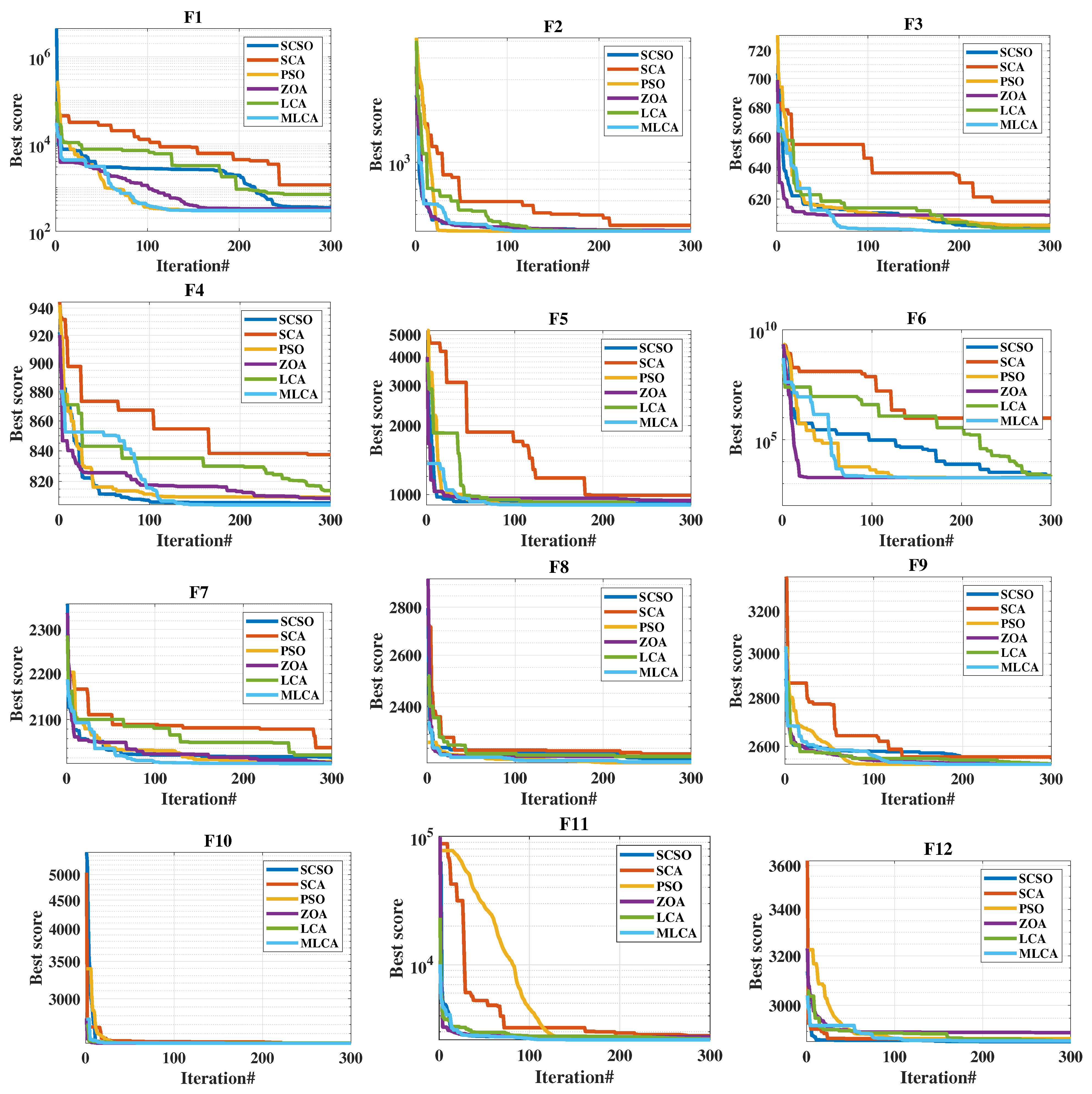
4.3.1. Application 1: Evaluation of the MLAC in Benchmark Functions

In this section, the performance of the proposed MLCA is tested and verified in CEC 2022 benchmark functions [83].

Table 3. Description of the CEC 2022 benchmark functions.

Function	Type	Fmin	Boundaries	Description
F1	Unimodal function	300	[−100, 100]	Shifted and full rotated Zakharov function
F2	Basic functions	400	[−100, 100]	Shifted and full rotated Rosenbrock’s function
F3		600	[−100, 100]	Shifted and full rotated expanded Schaffer’s F6 function
F4		800	[−100, 100]	Shifted and full rotated non-continuous Rastrigin’s function
F5		900	[−100, 100]	Shifted and rotated Levy function
F6	Hybrid functions	1800	[−100, 100]	Hybrid function 1 (N = 3)
F7		2000	[−100, 100]	Hybrid function 2 (N = 6)
F8		2200	[−100, 100]	Hybrid function 3 (N = 5)
F9	Composition functions	2300	[−100, 100]	Composite function 1 (N = 5)
F10		2400	[−100, 100]	Composite function 2 (N = 4
F11		2600	[−100, 100]	Composite function 3 (N = 5)
F12		2700	[−100, 100]	Composite function 3 (N = 5)

lists the description of the CEC 2022 benchmark functions. The obtained results by the MCLA are compared with other optimization methods including the Zebra optimization algorithm (ZOA) [84], Sand Cat swarm optimization (SCSO) [85], particle swarm optimization (PSO) [86], sine cosine algorithm (SCA) [87] and the conventional LCA. For a fair comparison, the maximum iterations and populations are selected to be 300 and 30, respectively, for all the studied algorithms and the other associated parameters are listed in

Table 4. The selected parameters of the chosen algorithms.

Algorithm	Parameter	Value
PSO	$t_{max}$, $Np$, $C1$, $C2$, $W1$	300, 30, 2,2, 0.7
SCSC	$t_{m}ax$, $Np$, Sensitivity range ($rg$), Phases control range (R)	300, 30, [2 - 0], [−2rg, 2rg]
SCA	$t_{max}$, $Np$, b	300, 30, [2 - 0]
ZOA	$t_{max}$, $Np$, R	300, 30, 0.01
LCA	$t_{max}$, $Np$	300, 30
MLCA	$t_{max}$, $Np$, $\delta$	300, 30, 4

.

4.3.2. Statistical Analysis

The efficacy of the MLCA is assessed through the statistical comparison with the other competitive optimization methods (SCSO, SCA, PSO, ZOA and the traditional LCA) in terms of the best, the average and the worst values of all types of CEC 2022 benchmark functions including the Unimodal, the basic, composition and hybrid benchmark functions. All statistical results were tabulated in

Table 5. The statistical results for the competitive algorithms with the proposed MLCA.

Function No.	Optimizer	Average	Best	Worst	SD
F1	SCSO	3093.775	349.1486	8691.832	2493.022
	SCA	3458.404	1164.057	6460.631	1667.455
	PSO	300.0105	300.0001	300.1228	0.024964
	ZOA	2406.967	323.1252	7635.127	2195.524
	LCA	1447.707	700.4051	3349.518	711.4054
	MLCA	300	300	300.001	0.000205
F2	SCSO	455.7817	401.0632	720.0985	68.29365
	SCA	494.0413	432.2709	542.0408	25.87232
	PSO	424.9348	400	471.3437	30.60353
	ZOA	476.7607	404.1804	910.9457	99.36141
	LCA	420.9453	401.0094	442.2129	12.7182
	MLCA	409.3691	400	470.8066	19.38046
F3	SCSO	619.4869	603.0549	640.0254	10.06907
	SCA	625.8878	618.392	649.0927	6.258529
	PSO	620.3777	603.8081	639.1443	10.40486
	ZOA	621.8001	610.0043	633.3335	5.858331
	LCA	605.1606	601.5796	610.2001	2.407723
	MLCA	603.0268	600.2005	611.2571	3.185232
F4	SCSO	829.3113	806.1021	844.7062	8.741245
	SCA	848.0268	837.5241	860.1306	6.503605
	PSO	821.6901	809.9496	842.7831	7.669336
	ZOA	816.5859	809.1074	830.5366	5.63061
	LCA	834.6409	814.102	854.8532	10.1297
	MLCA	825.3515	804.9748	832.8336	6.299992
F5	SCSO	1141.826	915.4967	1469.342	171.9704
	SCA	1083.895	992.3169	1283.928	80.46401
	PSO	1054.136	900	1362.665	153.0541
	ZOA	1061.449	940.9945	1283.71	96.35584
	LCA	923.2255	901.7043	963.4934	16.85943
	MLCA	909.5508	900.6334	957.7695	12.00111
F6	SCSO	4481.64	2187.17	8161.352	1751.289
	SCA	7439635	963067.3	26425791	7135852
	PSO	3052.999	1860.679	8084.839	1582.306
	ZOA	3100.627	1881.875	7298.885	1587.5
	LCA	21954.04	2048.434	136689.1	32740.4
	MLCA	1923.427	1828.147	2521.161	141.062
F7	SCSO	2048.494	2021.093	2089.621	18.7493
	SCA	2066.766	2041.341	2085.259	10.09232
	PSO	2044.901	2012.969	2094.026	21.58967
	ZOA	2053.452	2010.803	2114.428	22.98909
	LCA	2046.143	2026.291	2066.935	11.5397
	MLCA	2025.324	2008.956	2046.95	8.875774
F8	SCSO	2227.988	2214.531	2239.62	6.081599
	SCA	2239.191	2231.123	2251.613	5.328733
	PSO	2235.924	2200.537	2341.024	39.94917
	ZOA	2231.259	2222.731	2352.093	25.27378
	LCA	2229.289	2222.178	2231.57	2.287831
	MLCA	2219.969	2203.455	2224.124	4.350484
F9	SCSO	2594.81	2529.458	2678.021	35.10836
	SCA	2598.177	2557.816	2656.696	27.8627
	PSO	2541.842	2529.284	2676.216	40.64008
	ZOA	2614.066	2530.239	2718.711	45.68827
	LCA	2539.873	2531.308	2556.745	6.301353
	MLCA	2529.411	2529.284	2531.277	0.397224
F10	SCSO	2530.18	2500.426	2635.02	53.1725
	SCA	2528.239	2501.45	2673.45	58.37221
	PSO	2596.806	2500.387	2759.12	68.34379
	ZOA	2578.921	2500.553	2681.633	71.62236
	LCA	2500.802	2500.463	2501.487	0.222178
	MLCA	2500.435	2500.276	2500.703	0.1111
F11	SCSO	2831.009	2609.066	3309.952	170.1567
	SCA	3004.421	2793.088	3783.863	297.7186
	PSO	2953.419	2600.001	5230.808	485.1794
	ZOA	3053.657	2745.179	3430.171	182.3106
	LCA	2731.127	2636.21	2764.63	34.56173
	MLCA	2624.072	2600	2750.473	56.29244
F12	SCSO	2874.063	2861.454	2918.708	16.46731
	SCA	2873.296	2867.157	2891.819	4.697798
	PSO	2951.277	2872.847	3121.534	69.80949
	ZOA	2943.05	2895.543	3012.8	31.04917
	LCA	2869.805	2865.583	2875.687	2.388877
	MLCA	2871.416	2864.046	2898.943	7.599243

and the best-obtained values have been bolded. As seen in Table 5, the most competitive and superior results can be obtained by the application of the MLCA compared to SCA, SCSO, PSO, ZOA and the standard LCA. However, the PSO is the best for F5, F8 and F9 in terms of the best values.

4.3.3. Convergence Analysis

The convergence plotting can also be utilized to assess the performance of the suggested MLCA. Figure 10 shows the convergence plots of the MLCA with respect to SCA, SCSO, PSO, ZOA and the standard LCA. For the Unimodal (F1), the suggested MLCA is converged at 123th which is the best, compared to the other methods, in terms of the convergence speed and the accuracy. Likewise, for the basic, composition, and hybrid benchmark functions, the suggested optimizer converged rapidly before the 150th iteration except for F8; the PSO is the best.

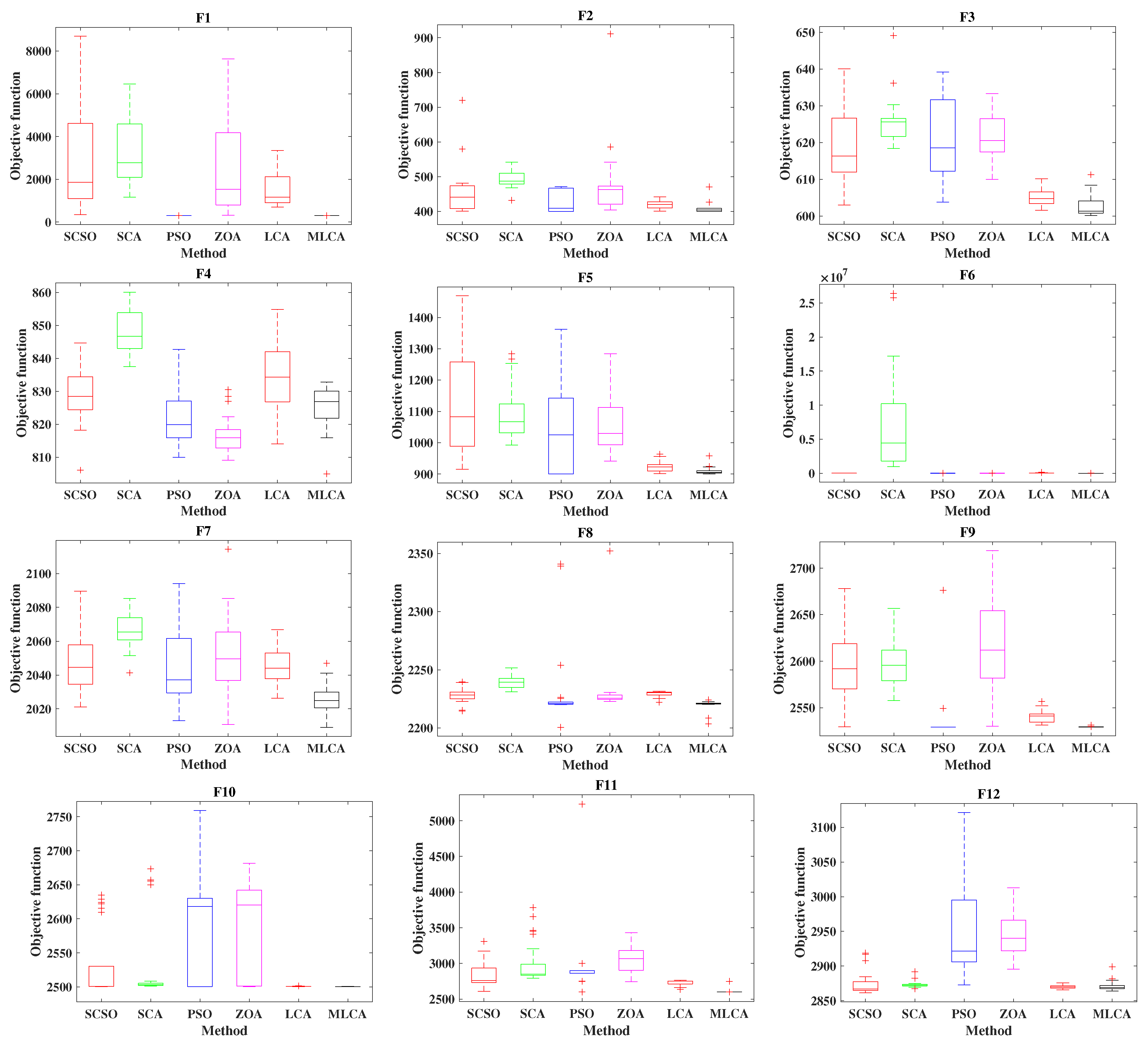
4.3.4. Boxplot Analysis

The boxplot is the third method that can be used for assessing the performance and efficacy of the MLCA with competitive techniques. The boxplot can provide the visual distribution of the obtained data from the reported optimizers. Figure 11 lists the boxplot for all objective functions by SCA, SCSO, PSO, ZOA standard LCA and the proposed MLCA. Judging from Figure 11, the suggested MLCA has the narrowest boxplot and interquartile range; its median is the lowest compared to other optimizers, which verifies that the MCLA is the best and superior compared to other algorithms.

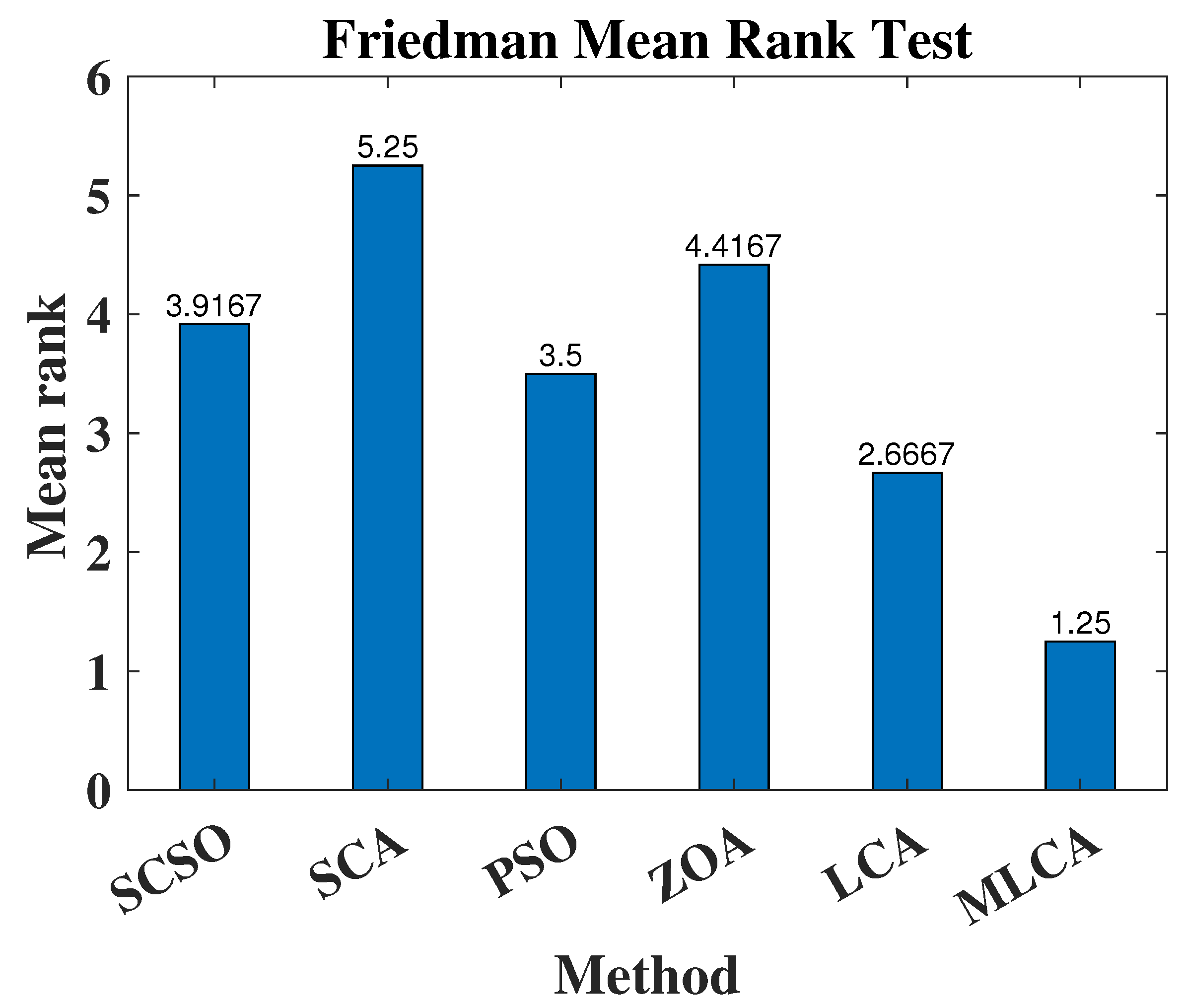
4.3.5. Wilcoxon and Fredman Tests

The Wilcoxon test is a robust statistical tool that is used to compare two data that are not normally distributed [88]. The p-value of the Wilcoxon test is the most important value that can describe if there is a high difference between the results or not. When the p-value is less than 0.05, this means that there is a meaningful difference, while when this value is more than 0.05 this means that there is no significant difference between the results.

Table 6. The p-values of Wilcoxon’s rank sum test for the MLCA with the other optimization methods.

MLCA vs.	SCSO	SCA	PSO	FOX	LCA
F1	1.4157 × 10−9	1.4157 × 10−9	5.2120 × 10−9	1.4157 × 10−9	1.4157 × 10−9
F2	9.6957 × 10−6	3.6690 × 10−9	1.1159 × 10−1	3.3440 × 10−7	8.1897 × 10−5
F3	9.2880 × 10−9	1.4157 × 10−9	1.3079 × 10−8	1.5967 × 10−9	1.6708 × 10−3
F4	8.7677 × 10−2	1.4055 × 10−9	1.8376 × 10−2	2.1373 × 10−5	9.6989 × 10−4
F5	2.2857 × 10−9	1.4157 × 10−9	2.9771 × 10−2	1.8002 × 10−9	3.3128 × 10−4
F6	2.5742 × 10−9	1.4157 × 10−9	3.2928 × 10−5	2.6597 × 10−6	2.0288 × 10−9
F7	1.6471 × 10−6	1.5967 × 10−9	1.1285 × 10−4	6.7951 × 10−7	1.0585 × 10−7
F8	3.7045 × 10−7	1.4157 × 10−9	8.0086 × 10−1	1.8002 × 10−9	2.0288 × 10−9
F9	1.8002 × 10−9	1.4157 × 10−9	1.5288 × 10−6	1.5967 × 10−9	1.4157 × 10−9
F10	2.5677 × 10−8	1.4157 × 10−9	2.4184 × 10−6	2.0288 × 10−9	1.6401 × 10−8
F11	1.3090 × 10−7	1.4157 × 10−9	8.2805 × 10−9	2.2857 × 10−9	3.0175 × 10−7
F12	1.8064 × 10−1	3.3915 × 10−3	1.0414 × 10−8	1.5967 × 10−9	5.7365 × 10−1

shows the p-vales of the proposed MLCA compared with SCSO, PSO, SCA, and the standard LCA. According to the outcomes of Table 6, most of the values are less than 0.05, which means that there are significant differences between the obtained results and between the studied optimization methods, except there is no significant difference between MLCA and SCSO for F12 and also between MLCA and PSO for F2 and F7. Likewise, there is no notable difference between MLCA and LCA for F12.

The Fredman test is a statistical tool that can be used to compare the results of multiple optimization methods and illustrates if there is a notable difference in the mean ranks of the optimizers’ outcomes [89]. Figure 4 shows the results of the Fredman test of MLCA, LCA, SCSO, SCA, PSO, and ZOA. Judging from Figure 4, the ranking of the MLCA, LCA, SCSO, SCA, PSO, and ZOA based on the mean rank values are 1, 2, 4, 6, 3 and 5, respectively. It is clear that the MCLA is a robust and superior technique compared to other optimization methods.

The Fredman test is a statistical tool that can be used to compare the results of multiple optimization methods and illustrates if there is a notable difference in the mean ranks of the optimizers’ outcomes [89]. Figure 12 shows the results of the Fredman test of MLCA, LCA, SCSO, SCA, PSO, and ZOA. Judging from Figure 12, the ranking of the MLCA, LCA, SCSO, SCA, PSO, and ZOA based on the mean rank values are 1, 2, 4, 6, 3 and 5, respectively. It is clear that the MCLA is a robust and superior technique compared to other optimization methods.

4.4. The Proposed MLCA-Based Control Parameters Optimization Process

The proposed 1+TD/FOTIDF LFC possesses nine parameters in the MG area a ($K_{t1}$, $K_{d1}$, $n_1$, $K_{t2}$, $n_2$, $K_{i1}$, ${\lambda }_1$, $K_{d2}$, and $N_{c2}$). Also, the MG area b has another nine parameters ($K_{t3}$, $K_{d3}$, $n_3$, $K_{t4}$, $n_4$, $K_{i2}$, ${\lambda }_2$, $K_{d4}$, and $N_{c2}$). A total of 18 tunable design parameters in the proposed 1+TD/FOTIDF LFC method is summarized in

Table 7. The optimum parameters using MLCA optimizer.

Controller	Area	Parameters
		${\mathit{K}}_{\mathit{t}\mathbf{1}}$	${\mathit{K}}_{\mathit{i}\mathbf{1}}$	${\mathit{K}}_{\mathit{d}\mathbf{1}}$	${\mathit{n}}_{\mathbf{1}}$	${\mathit{K}}_{\mathit{t}\mathbf{2}}$	${\mathit{K}}_{\mathit{i}\mathbf{2}}$	${\mathit{K}}_{\mathit{d}\mathbf{2}}$	${\mathit{n}}_{\mathbf{2}}$	${\mathit{\lambda }}_{\mathbf{1}}$	${\mathit{\mu }}_{\mathbf{1}}$	${\mathit{N}}_{\mathit{f}\mathbf{1}}$
FOTID	a	2.245	1.987	1.713	2.234	―	―	―	―	0.622	0.574	―
	b	2.956	2.016	0.895	2.923	―	―	―	―	0.714	0.882	―
TI/FOTID	a	3.155	2.019	―	2.862	2.868	3.036	1.156	3.634	0.882	0.857	―
	b	2.738	1.583	―	3.235	2.365	2.678	1.344	3.69	0.566	0.843	―
TD/FOTID	a	3.928	―	1.037	3.555	4.018	3.346	2.147	3.944	0.788	0.948	―
	b	3.748	―	1.164	4.022	3.571	3.176	2.291	3.891	0.758	0.788	―
1+TD/FOTIDF	a	4.525	―	3.851	4.576	4.864	3.865	3.998	4.977	0.948	0.877	151.36
	b	4.118	―	4.073	4.281	3.954	4.279	3.092	4.583	0.882	0.915	189.5

. The proposed MLCA is employed for determining optimum values for the 18 parameters simultaneously for obtaining the best performance and disturbance rejections. The main directing factor for the optimization algorithm is the selected objective function of the process. The main four objectives for LFC design are integral-squared errors (ISE), integral-absolute errors (IAE), integral-time-squared errors (ITSE), and integral-time-absolute errors (ITAE). Their general representations are as follows:

$$\begin{array}{c}ISE=\int {\displaystyle \sum _{i=1}^m}\left(e_i^2\right)\mathrm{d}t\\ IAE=\int {\displaystyle \sum _{i=1}^m}abs\left(e_i\right)\mathrm{d}t\\ ITSE=\int {\displaystyle \sum _{i=1}^m}\left(e_i^2\right)t.\mathrm{d}t\\ ITAE=\int {\displaystyle \sum _{i=1}^m}abs\left(e_i\right)t.\mathrm{d}t\end{array}$$

(75)

The directing objective function for interconnected MGs includes the minimization of frequency deviations in each connected area (in the studied case, minimizing $\Delta f_a$ and $\Delta f_b$). Additionally, the minimization of tie-line power deviations between connected areas (in the studied case minimizing $(\Delta P_{tie})$). The three objectives in the studied case include $\Delta f_a$, $\Delta f_b$, and $(\Delta P_{tie})$. They are combined in a single objective function. Using definitions of ISE, IAE, ITSE, and ITAE objectives in Equation (75), the objective functions can be formulated as:

$$\begin{array}{c}ISE=\underset{0}{\overset{t_s}{\int }}({(\Delta f_a)}^2+{(\Delta f_b)}^2+{(\Delta P_{tie})}^2)\mathrm{d}t\\ IAE=\underset{0}{\overset{t_s}{\int }}(abs(\Delta f_a)+abs(\Delta f_b)+abs(\Delta P_{tie}))\mathrm{d}t\\ ITSE=\underset{0}{\overset{t_s}{\int }}({(\Delta f_a)}^2+{(\Delta f_b)}^2+{(\Delta P_{tie})}^2)t.\mathrm{d}t\\ ITAE=\underset{0}{\overset{t_s}{\int }}(abs(\Delta f_a)+abs(\Delta f_b)+abs(\Delta P_{tie}))t.\mathrm{d}t\end{array}$$

(76)

The process of parameter optimization is constrained by the following ranges for each tunable parameter:

$$\begin{array}{c}{K}_t^{min}\le K_{t1},K_{t2}\le K_t^{max}\\ K_i^{min}\le K_{i1},K_{i2}\le K_i^{max}\\ K_d^{min}\le K_{d1},K_{d2}\le K_d^{max}\\ {\lambda }^{min}\le {\lambda }_1,{\lambda }_2\le {\lambda }^{max}\\ { }^{min}{\le }_1{,}_2{,}_3{,}_4\le {\mu }_c^{maxmin}{\le }_{c1}{,}_{c2}{\le }_c^{max}\end{array}$$

(77)

In which, ${\left(f\right)}^{max}$ and ${\left(f\right)}^{min}$ are referred to upper, and lower constraints, respectively, for tunable parameters. Lower limiting constraints for ($K_t^{min}$, $K_i^{min}$, $K_d^{min}$) are selected at zero, and upper ones ($K_t^{max}$, $K_i^{max}$, $K_d^{max}$) are selected at 5 in the proposed process. FO operator $\lambda$ possesses a lower value ${\lambda }^{min}$ at 0 and its upper one ${\lambda }^{max}$ is selected at 1. The tilt operator n is set in the range [2–10] and $N_c$ is set in the range [5–300]. Figure 13 shows the proposed MLCA-based parameters optimization method.

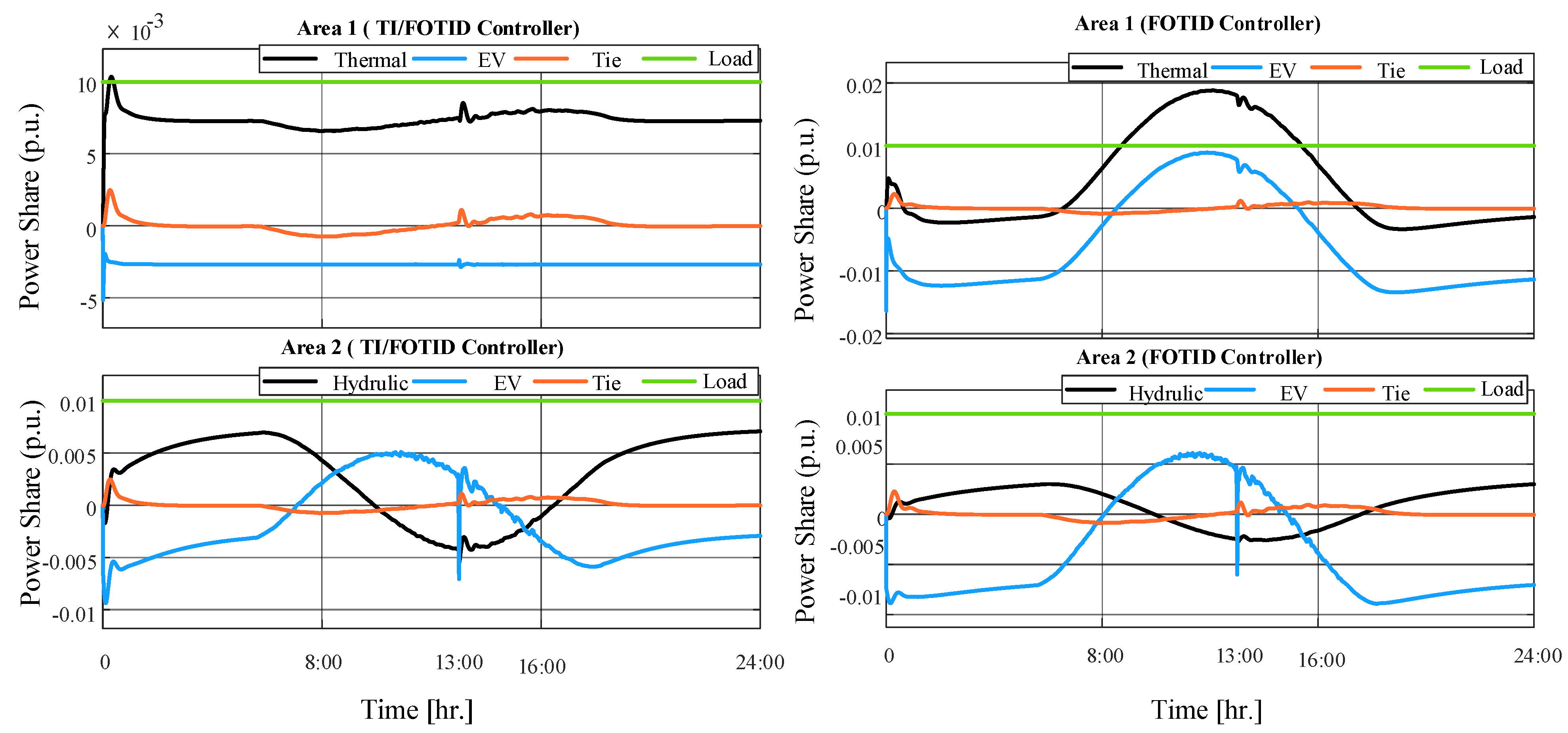
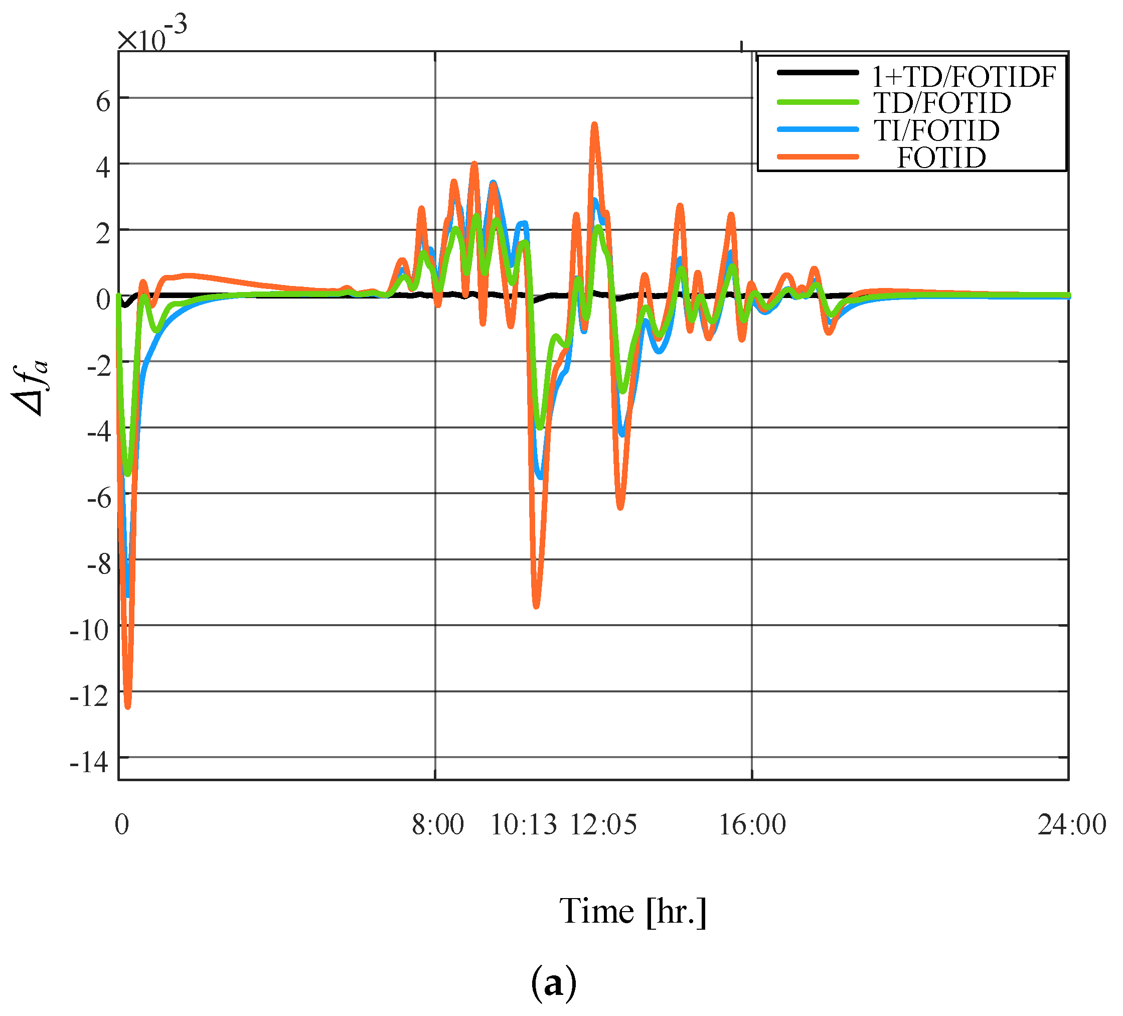
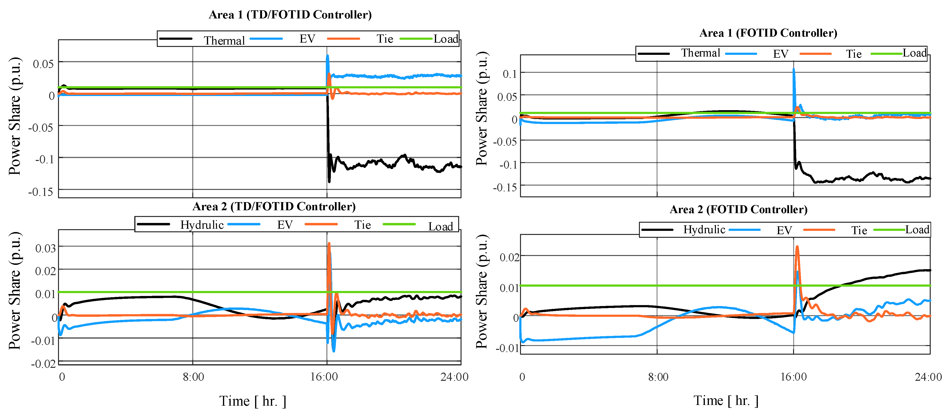
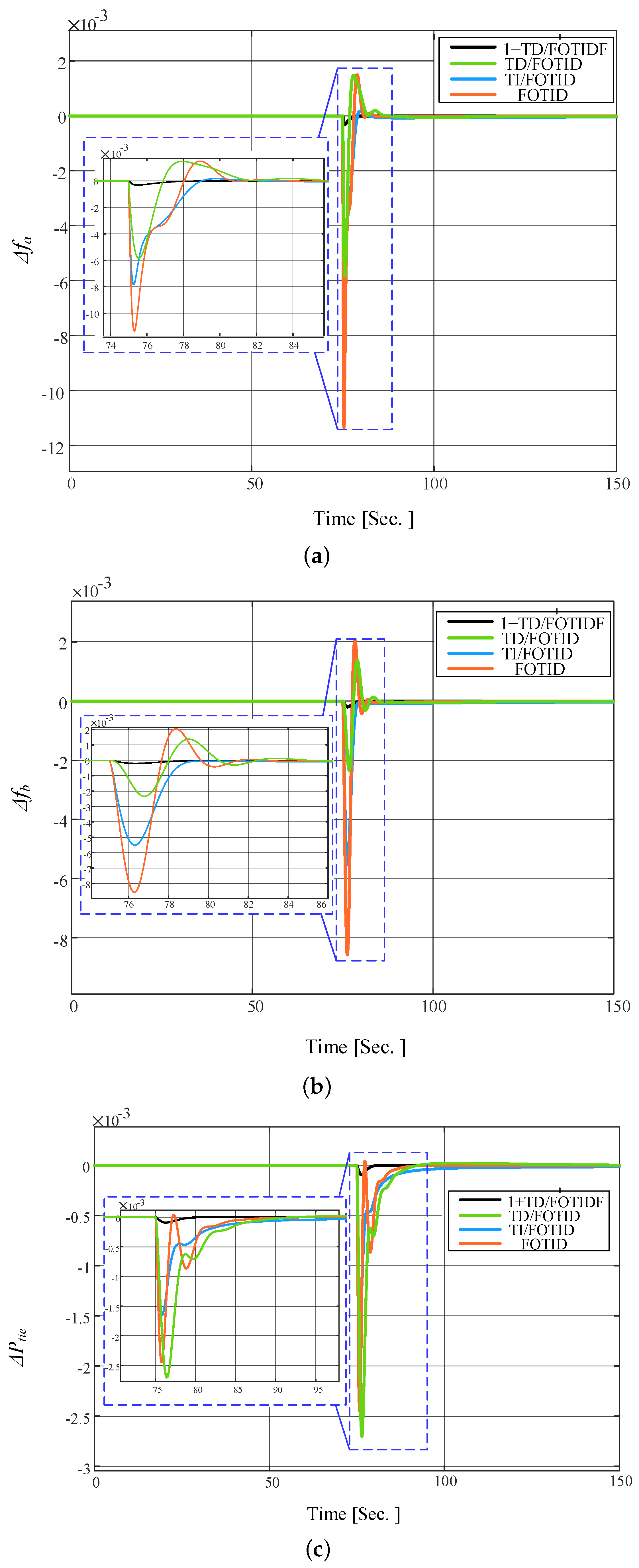
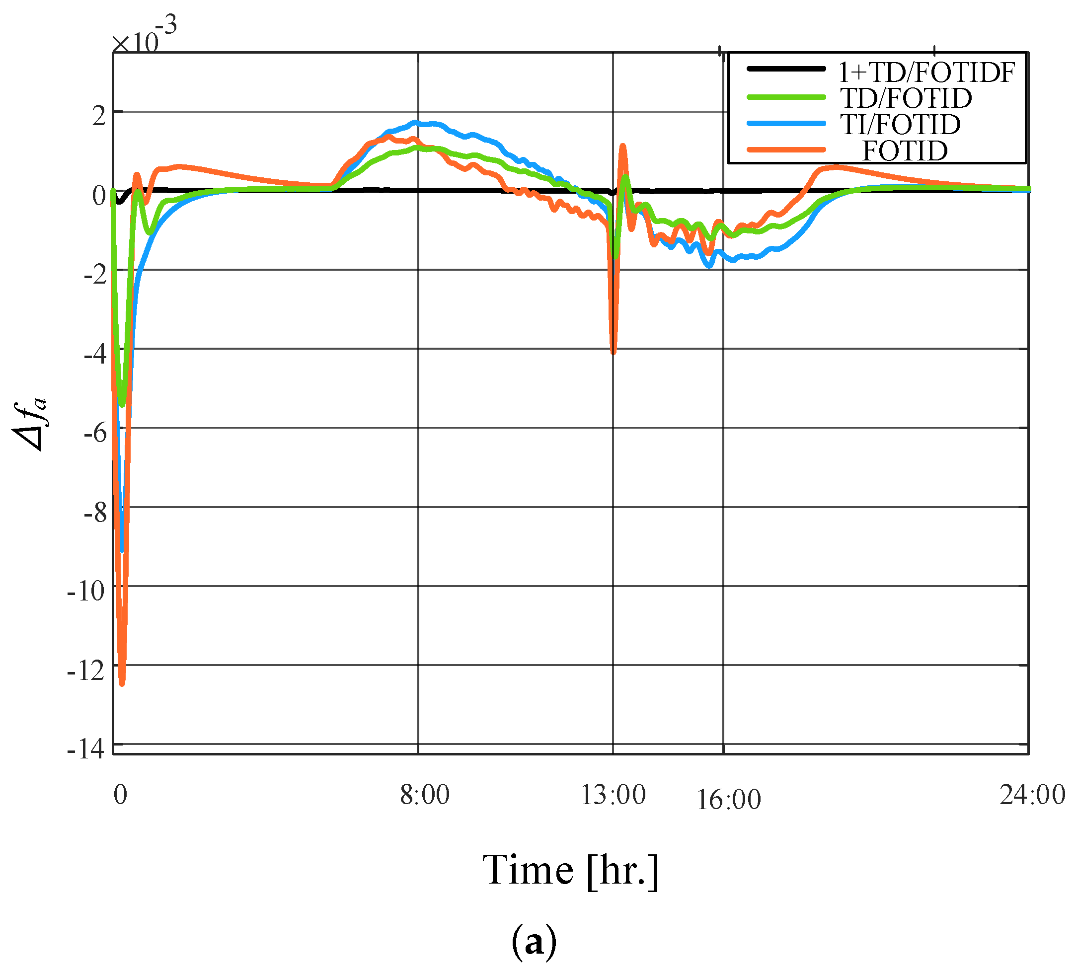
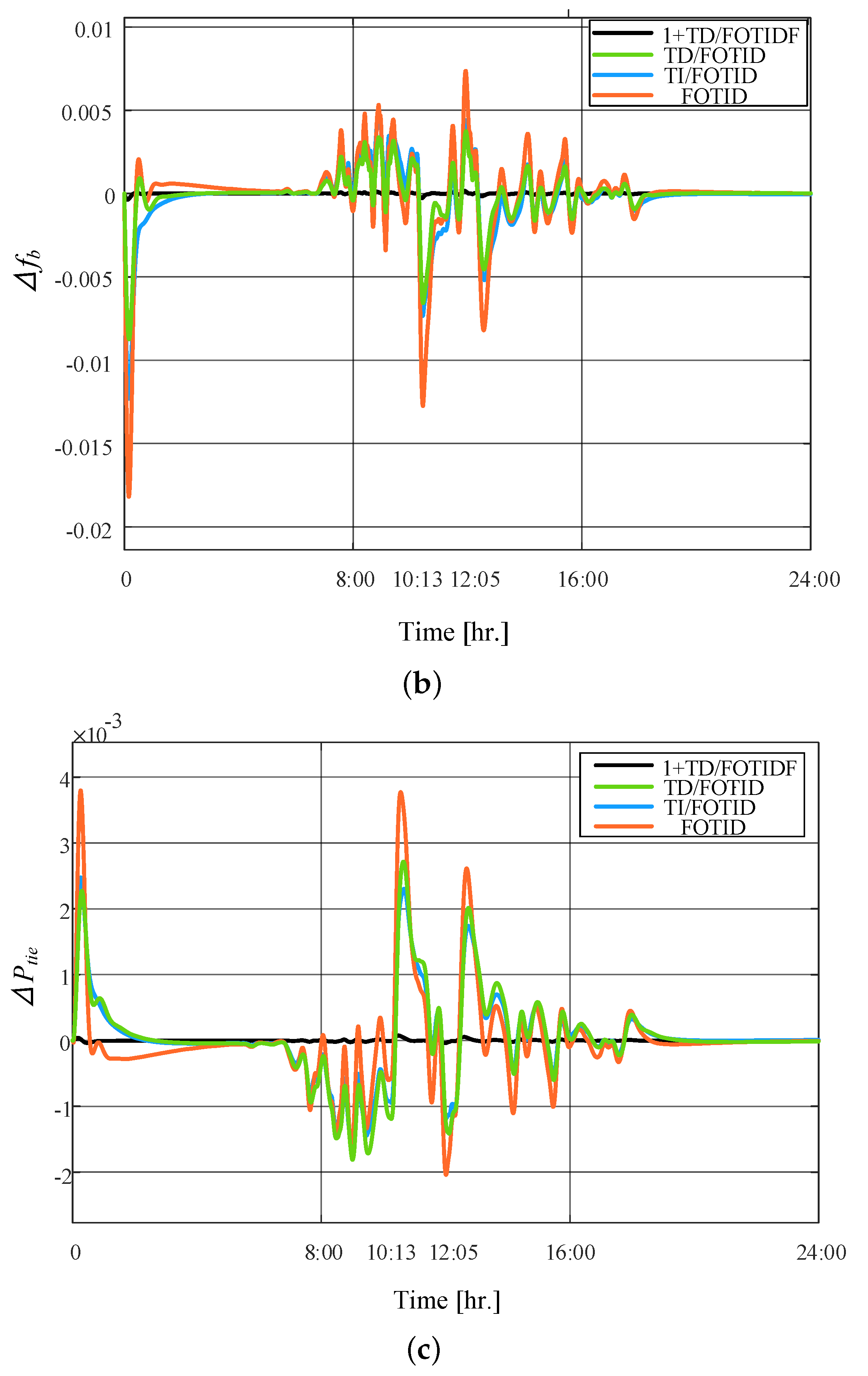
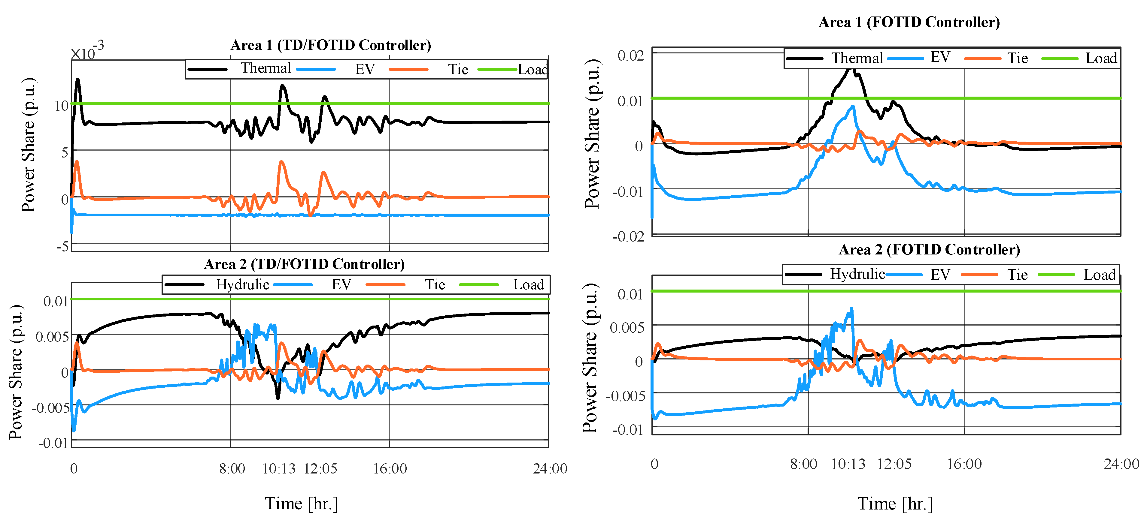
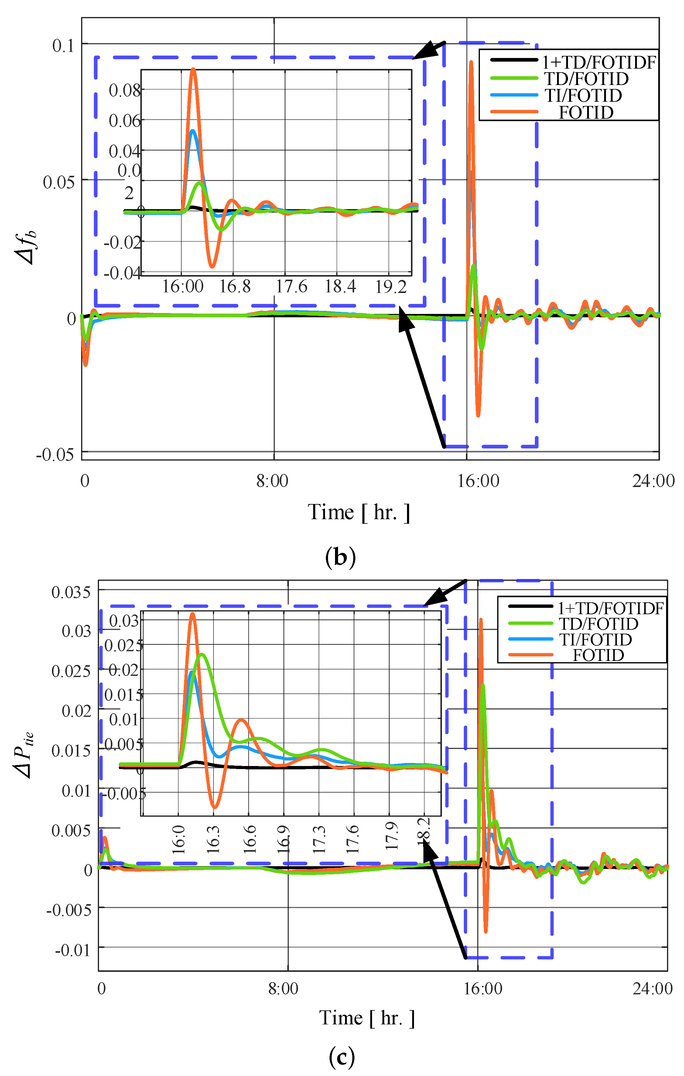
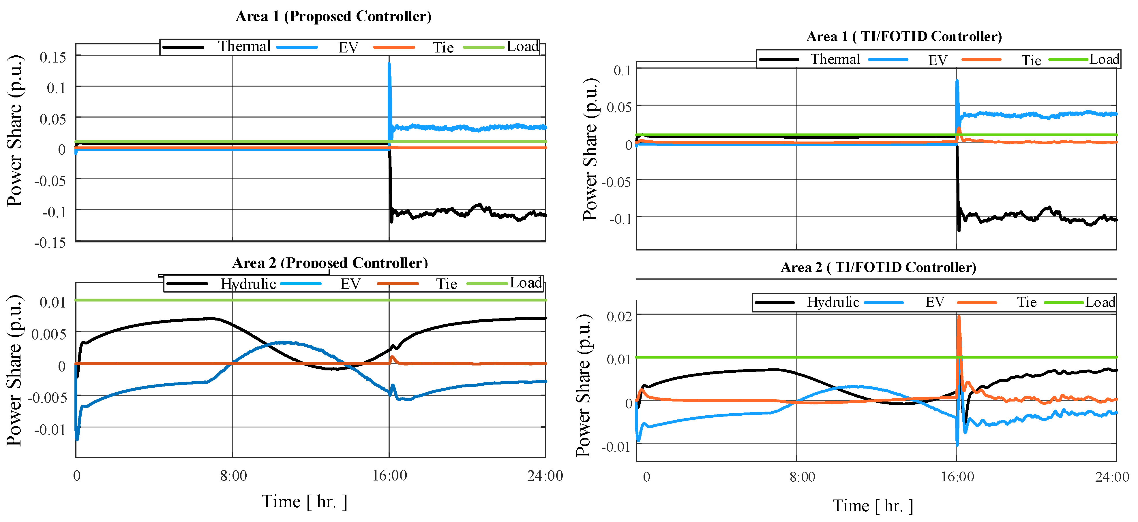
5. Results and Discussions

The programming code for tuning the proposed CC 1+TD/FOTIDF controller based-MLCA algorithm has been implemented using a MATLAB m-file via a personal computer with an Intel® i7 1.9 GHz processor and 12 GB RAM (HP, iyadh, Saudi Arabia). This code is interfaced with the Simulink model of the dual area MG power system to execute the optimization process with a twenty populations number and one hundred iterations to tune the parameters of the suggested CC 1+TD/FOTIDF, TD/FOTID, TI/FOTID, and FOTID controllers. Furthermore, the convergence performance of the MLCA code is examined and compared with the other algorithms, such as SCA, SCSO, PSO, ZOA, and LCA, as shown in Figure 10, which proves that the MLCA technique has a faster convergence rate with a smoother curve compared to meta historical methods. To approve the proposed scheme validation and the investigated algorithm, the dual area MG power system has been conducted under identical operating scenarios such as step load change (SLC) and different cases of PV irradiation conditions and wind speed variations. In these scenarios, the stability and frequency variation responses of the proposed control technique are compared to those of conventional and fractional controllers to evaluate its superiority. It should be noted that the scenarios of PV penetration are based on real solar radiation data. The measurements of global solar radiation were acquired from the King Abdullah City for Atomic and Renewable Energy (KACARE), the primary authorized organization responsible for gathering and overseeing data on renewable energy resources in Saudi Arabia. These scenarios are organized as follows:

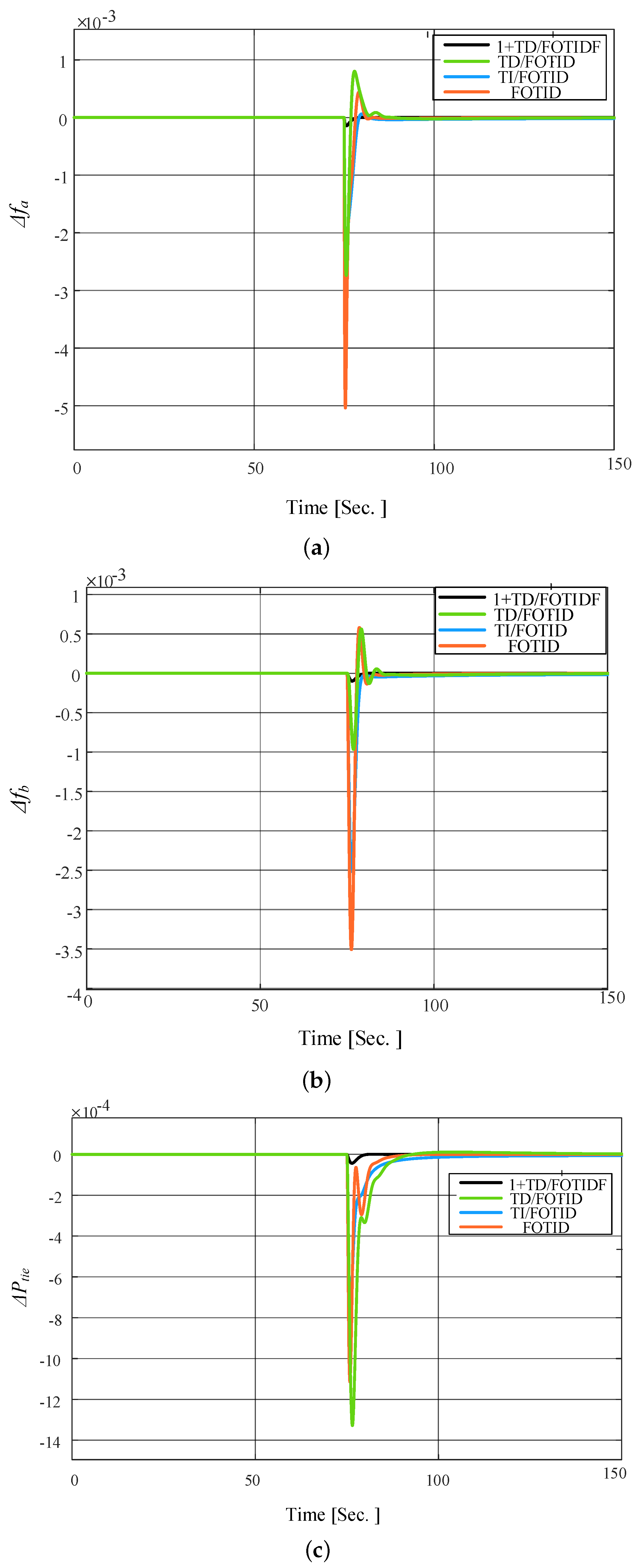
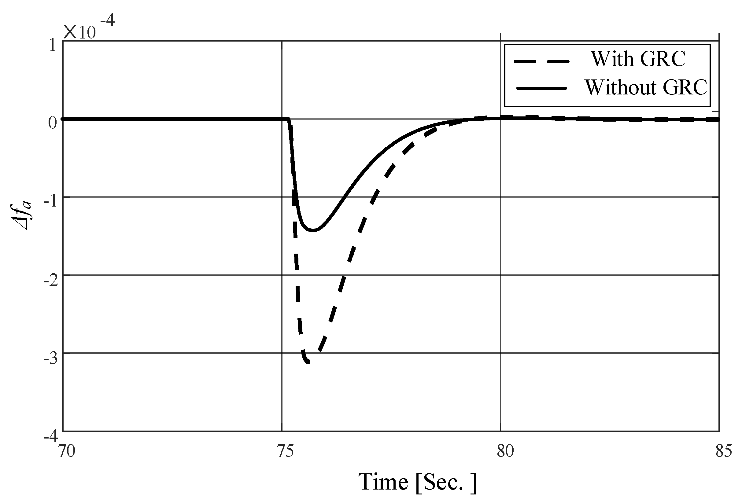
5.1. Scenario 1: 2% Step Load Change (SLC)

The proposed CC 1+TD/FOTIDF controller based on the MLCA is investigated by employing 2% SLC at time t = 75 s in area a without using RESs in the studied dual area microgrid system considering the GRC. Figure 14 presents the waveforms of change rate in interconnected line power and system frequency in the dual areas a and b for the studied multi-area power network. This scenario tests the various control patterns such as FOTID, TI/FOTID, TD/FOTID, and proposed CC controllers based on the MLCA for simulation intention via the influence of a 2% SLP. It is spotted from this figure that the MLCA-based CC 1+TD/FOTIDF control, with the percentage participation of the EV, offers remarkable performance with an amazing decrease in frequency and power deviations compared to other traditional and fractional control structures. The value of the frequency deviation of the investigated MG network with the FOTID controller has been maintained at 0.0115 Hz for area a and 0.0082 Hz for area b, with an interconnected-line power deviation within 0.0028 p.u in this status. According to the TI/FOTID, the system frequency has been kept to 0.0079 Hz for area a and 0.0058 Hz for area b and the perversion of interconnected-line power is 0.0024 p.u during the perturbation of a 2% load change at 75 s instant. However, the results obtained from the TD/FOTID controller were acceptable regarding the previous two controllers. In contrast, the tie-line power is 0.0016 p.u and the frequency reached 0.0058 Hz for area a and 0.0023 Hz for area b. Conversely, the CC 1+TD/FOTID has a strong performance by reducing the network frequency variation of the investigated dual area MG system to 0.0001 Hz for area a and 0.0005 Hz for area b while maintaining the power deviation at 0.00008 p.u. The numerical estimations of the examined MG system’s dynamic restraint in terms of maximum and minimum overshoots and settling time for step load adjustment are summarized in

Table 8. The obtained results for the tested scenarios.

Scenario	Controller	$\mathbf{\Delta }{\mathit{f}}_1$ (P.U)			$\mathbf{\Delta }{\mathit{f}}_2$ (P.U)			$\mathbf{\Delta }{\mathit{P}}_{\mathit{tie}}$ (P.U)
		PO	PU	ST (s)	PO	PU	ST (s)	PO	PU	ST (s)
No.1 at 75 s	FOTID	0.0019	0.0115	17	0.0021	0.0082	16	0.0005	0.0028	22
	TI/FOTID	0.0002	0.0079	9	0.0016	0.0058	20	0.0001	0.0024	18
	TD/FOTID	0.0017	0.0058	15	0.0001	0.0023	10	0.0002	0.0016	10
	1+TD/FOTIDF	-	0.0001	4	-	0.0005	5	-	8.4 × 10−5	6
No.2 at 8:00 AM.	FOTID	0.0016	0.0012	FU	0.0017	0.0011	FU	0.0004	0.0005	FU
	TI/FOTID	0.0017	0.0018	FU	0.0019	0.0015	FU	0.0006	0.0007	FU
	TD/FOTID	0.0008	0.0009	FU	0.0005	0.0007	FU	0.0007	0.0009	FU
	1+TD/FOTIDF	1 × 10−6	1 × 10−5	FU	1.1 × 10−6	1.01 × 10−5	FU	1 × 10−6	1.1 × 10−6	FU
No.3 at 13:00 PM.	FOTID	0.0012	0.0042	FU	0.0025	0.0073	FU	0.0016	0.0004	FU
	TI/FOTID	0.0011	0.0023	FU	0.0019	0.0041	FU	0.0011	0.0003	FU
	TD/FOTID	0.0001	0.0021	FU	0.0014	0.0037	FU	0.0009	0.0001	FU
	1+TD/FOTIDF	1 × 10−5	1 × 10−5	FU	0.9 × 10−5	1 × 10−6	FU	1 × 10−4	1 × 10−6	FU
No.4 at 10:00 AM.	FOTID	0.0057	0.0099	FU	0.0072	0.0133	FU	0.0039	0.0021	FU
	TI/FOTID	0.0028	0.0058	FU	0.0041	0.0033	FU	0.0022	0.0013	FU
	TD/FOTID	0.002	0.004	FU	0.0036	0.0031	FU	0.0021	0.0011	FU
	1+TD/FOTIDF	0.0001	0.0004	FU	0.0001	0.0001	FU	1 × 10−4	1 × 10−5	FU
No.5 at 16:00 PM.	FOTID	0.141	0.022	FU	0.123	0.0392	FU	0.033	0.0067	FU
	TI/FOTID	0.0826	0.0018	FU	0.0524	0.0141	FU	0.0192	0.0031	FU
	TD/FOTID	0.0522	0.0151	FU	0.0198	0.011	FU	0.022	0.0023	FU
	1+TD/FOTIDF	0.004	-	120	0.001	-	110	0.0013	-	180

FU = Fluctuated.

. When compared to other controllers, the CC 1+TD/FOTID controller, which is based on the MLCA, performs exceptionally well. From another side, Figure 15 shows that the MG system is simulated without considering the GRC limits at the same operation. It can be observed that not utilizing the GRC results in a lower peak undershoot and a smaller settling time for all the suggested controllers. Furthermore, the performance of the proposed controller with and without the GRC limits is depicted in Figure 16, which indicates the deterioration of the system’s dynamic performance. Therefore, a GRC limit must be included for the realistic study of the MG system.

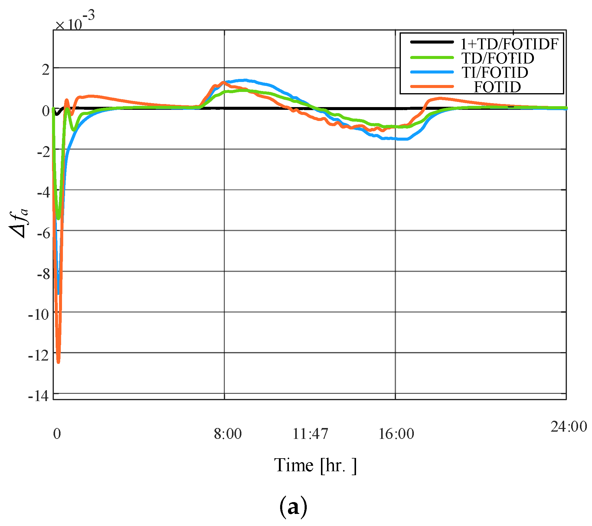
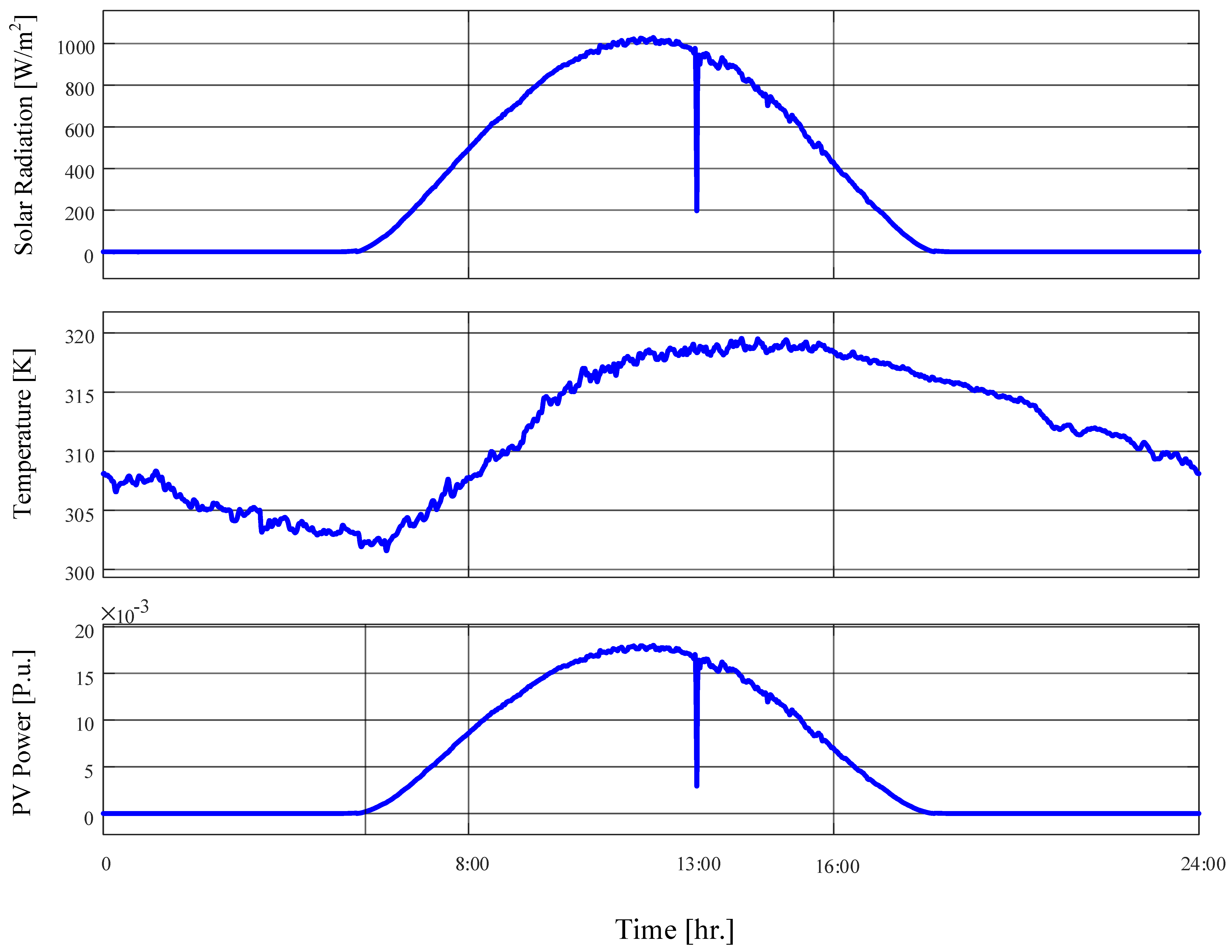
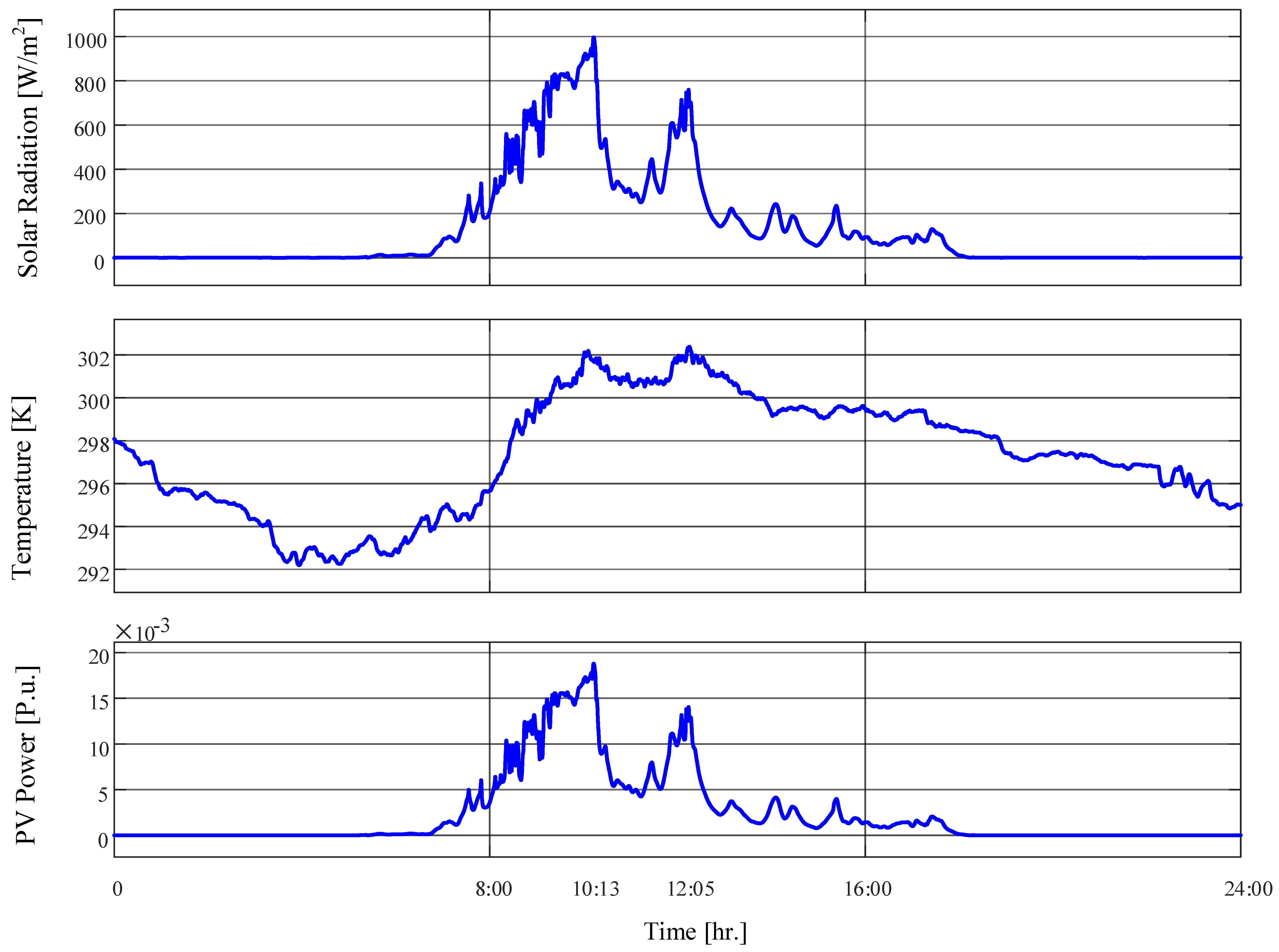
5.2. Scenario 2: SLC with PV Irradiation Case A

At the same load profiles of the previous scenario, a 24 h practical PV profile is integrated at area b, in this case, to examine the performance of the suggested CC 1+TD/FOTID, FOTID, TI/FOTID, and TD/FOTID control structures under the variation conditions of solar units. The PV irradiance, temperature, and power profiles are shown in Figure 17 for this scenario. Figure 18 and Table 8 show the control response results of this case. This table proves that the CC proposed controller has the ability to obtain the lowest value of frequency deviancy compared to the FOTID controller, the TI/FOTID controller, and the TD/FOTID controller. Furthermore, it has the best damping characteristics in frequency and tie-line power deviations at SLC and during increasing and decreasing periods of PV power compared to other characteristics from other controllers as shown in Figure 18. Conversely, the control signal provided by the planned CC 1+TD/FOTID controller achieved faster EV performance, high EV discharge and less power consumption from the traditional thermal and hydraulic units than the other controllers. As a result, it is clear from this illustration that the new MLCA technique-based suggested that the CC 1+TD/FOTID controller is the most reliable one in that particular LFC scenario.

5.3. Scenario 3: SLC with PV Irradiation Case B

For the validation of the proposed CC 1+TD/FOTID controller, which is fine-tuned by the MLCA technique, the simulation experiments of this scenario have been accomplished under the two SLCs in both areas for 2%, besides a severe cloudy condition of the PV power generation which is attained from the incoming irradiance and temperature profiles for 24 h in Figure 19. This PV profile has a severe drop in its power value at t = 1:00 PM, which reflects the robustness and efficacy of the proposed CC controller. Figure 20 shows a contrast effect of the investigated controllers in terms of frequency and power deviations of the dual area MG system. It is noteworthy that the proposed controller displays greater genealogical stability than the other techniques of control. This figure implies that the aberration of the frequency with the CC 1+TD/FOTID controller is less than ±0.00005 Hz at the initial time of simulation and less than ±0.00002 Hz at the instant of the cloudy period, which causes a significant power drop of PV units. While the deviation with FOTID, TI/FOTID, and TD/FOTID arrives at ±0.012 Hz, ±0.009 Hz and 0.005 Hz at t = 0 s, respectively, and at ±0.004 Hz, ±0.003 Hz and 0.002 Hz at cloudy times, respectively, in area a. Furthermore, the effectiveness of the new CC controller can be noted in Figure 21, which proves that the required power from thermal generation during load and PV variations using the CC 1+TD/FOTID is smaller than with the other controllers, and that specifies the role of the proposed technique. In addition, the different performance effect of the four controllers on the EV action is depicted in Figure 21. It indicates that the proposed method presents a large and fast charge/discharge process compared with the other three techniques. Therefore, these results prove that the inner loop of the proposed CC controller responds instantly to the dynamics initiated by PV power and other generation sources in the dual area system, as well as the outer control loop, which can handle the load perturbations and system dynamics.

5.4. Scenario 4: SLC with sever PV Irradiation Case C

The capability of the suggested CC 1+TD/FOTIDF LFC coordinated with EVs based on the MLCA technique is assessed and demonstrated under an extreme disturbance condition from the PV units. Solar power has a very bad irradiation output, which causes severe power oscillations in this case, as depicted in Figure 22. Therefore, this scenario became a great challenge facing the suggested LFC techniques. Figure 23 shows the acquired frequency and interconnected-line power variations of the investigated dual area microgrid system for this situation. It can be observed that the CC 1+TD/FOTIDF control comes first in reducing the frequency and power aberrations in contrast to alternative control methods. It can dampen the system frequency oscillations smoothly within 0.0004 Hz for area a and 0.0001 Hz for area b and maintain tie-power change within 0.0001 p.u during severe periods of PV irradiance fluctuations at 10 AM. The TD/FOTID came in the second order with frequency deviating at 0.004 Hz for area a, 0.0031 Hz for area b, and ±0.0011 p.u for grid frequencies and interconnected-line power, respectively. TI/FOTID comes thirdly by upholding the frequency deviancy at 0.0058 Hz for area a and 0.0033 Hz for area b and keeping tie-line power value within 0.0013 P.U. While the FOTID controller comes last, it has the highest overshoot and undershoot in frequency diffraction within 0.0099 Hz for area a and 0.0133 Hz for area b and keeps tie-line power change within 0.0021 p.u compared to the proposed one and other traditional controllers. From another side, Figure 24 shows the feature of the dual loops of the CC 1+TD/FOTIDF technique in controlling the discharge from the EV and required power from thermal and hydraulic generators with respect to other control methods.

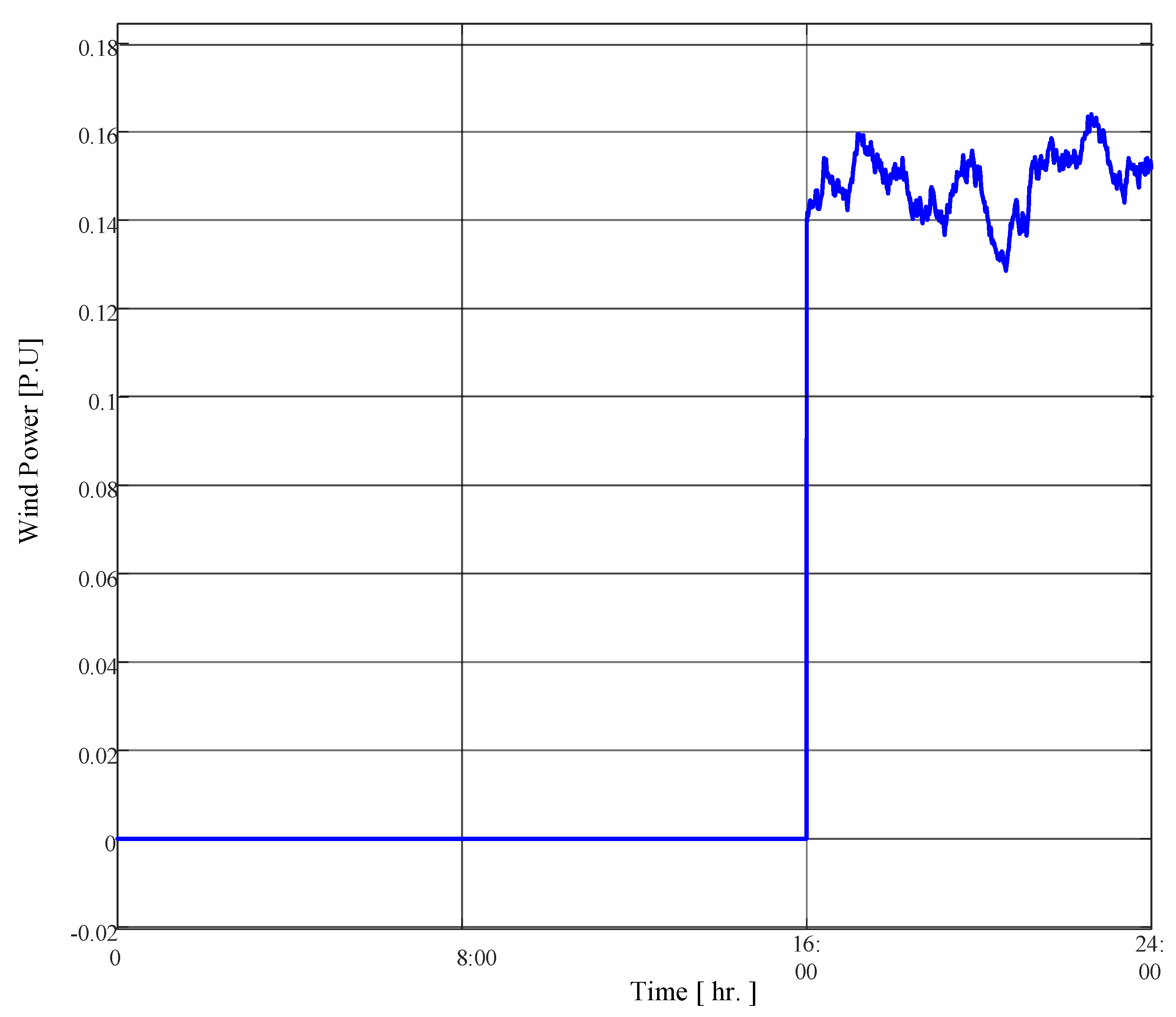
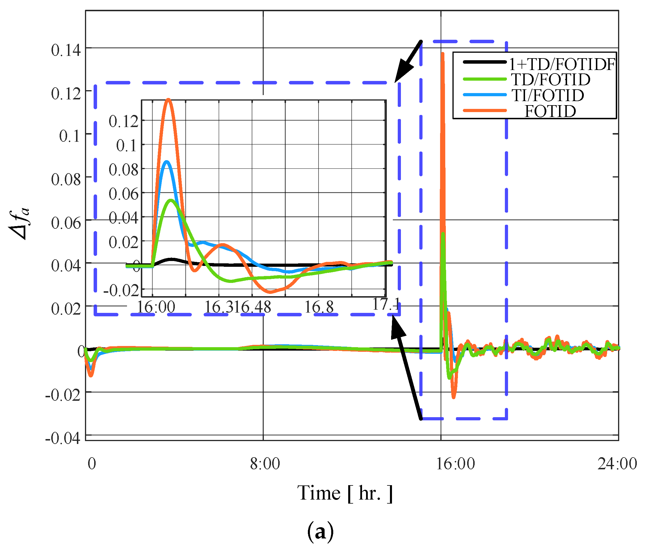
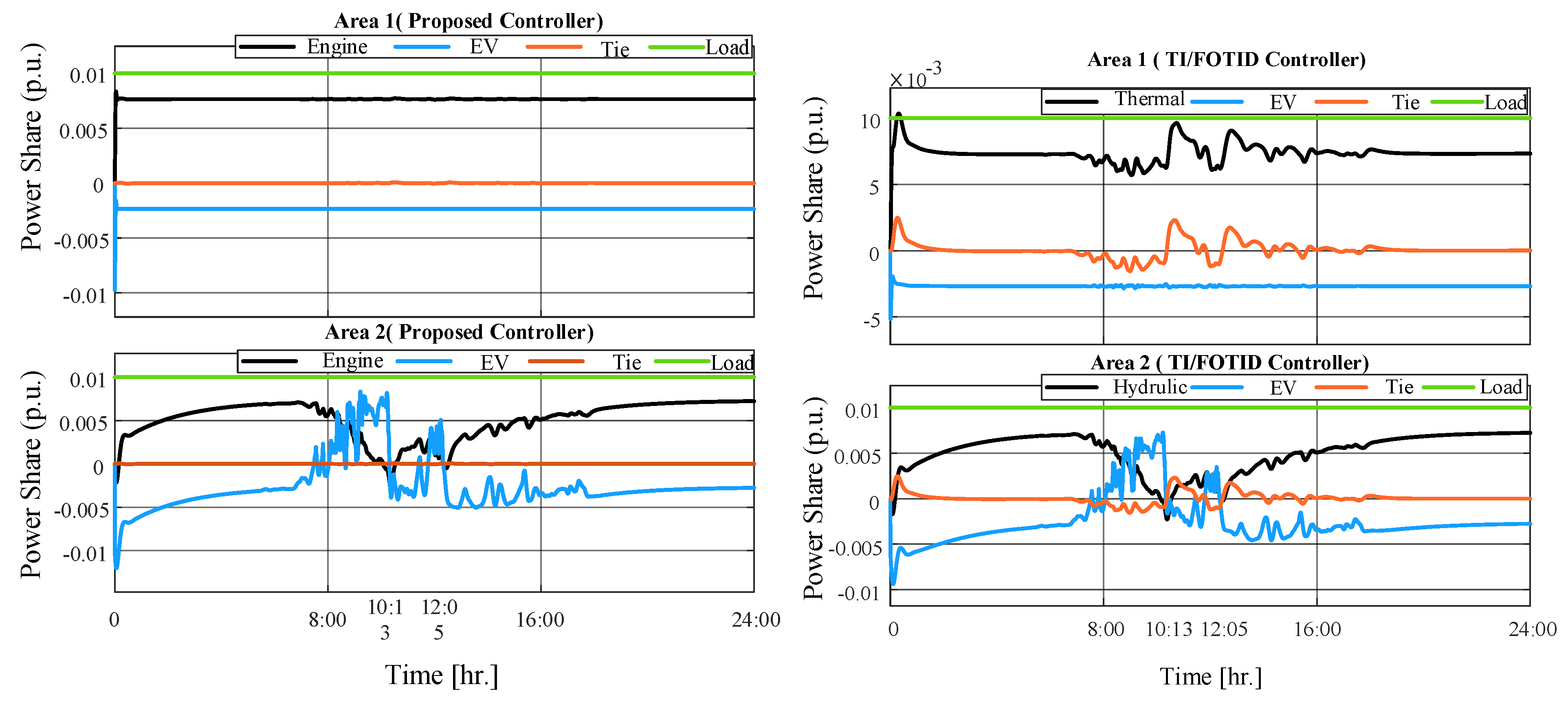
5.5. Scenario 5: High RESs of PV and Wind Generation

In this case, the electric generation of the dual area MG is increased by adding a wind generation farm. Its profile is shown in Figure 25. However, a power imbalance in the MG system can occur due to the uncertainty in the wind speed which in turn causes severe frequency and power fluctuations. Therefore, this scenario takes into consideration the highly fluctuating wind power besides the integration of PV power and load change impacts of scenario 2 on the investigated power grid. The contrast performance of the four suggested controllers on the studied dual area MG system is shown in Figure 26. The FOTID controller has a sharp frequency reverberation up to 0.141 Hz and 0.123 Hz in areas a and b, respectively, at the wind integration instant. The TI/FOTID controller presents a large peak frequency diffraction to 0.0826 Hz at area a and 0.0524 Hz at area b when there is an upsurge in active power from the wind farm due to its uncertainty velocity. The TD/FOTID gave satisfactory results compared with FOTID and TI/FOTID controllers. It can dampen the frequency perversion at 0.052 Hz at area a and 0.0198 Hz at area b. On the contrary, the proposed CC 1+TD/FOTIDF control technique manifested an outstanding performance against wind uncertainty. It can reduce the deviation in system frequency to 0.004 Hz and 0.001 Hz in both areas. This is because the CC 1+TD/FOTIDF does not have a phase lag in responding to different generation and load disturbances compared to other single-loop controllers. Furthermore, the proposed cascaded controllers proved their superiority to the fast charge and discharge from the EVs in both areas. Figure 27 shows that the control signal from the proposed technique accomplished reducing the power from the thermal and hydraulic powers with a quick discharge from the EV system, especially at instants of increasing/decreasing the PV power and integration of the wind farm to the dual area MG system comparing with other conventional and fractional controllers.

6. Conclusions

The integration of improperly controlled renewable energy resources and electric vehicles into the power system might result in frequency fluctuations, leading to desynchronization and ultimately compromising the stability of the power system. Numerous LFC techniques have been proposed in the literature to regulate the system frequency at a stable level. The paper introduces an improved version of a PID controller with fractional order. The proposed controller is a cascaded controller comprising a 1+TD inner controller and an outer controller with a FOTIDF controller, resulting in a 1+TD/FOTIDF controller. The proposed controller exhibits an effective capacity to reject both existing generations and load disturbances, hence enhancing the stability of the multi-microgrids under imbalanced power conditions. Moreover, the proposed 1+TD/FOTIDF controller effectively manages the involvement of the electric vehicle’s batteries and helps mitigate disruptions in the power system frequency. Furthermore, a new MLC optimization approach is introduced to enhance the parameters of the 1+TD/FOTIDF controller in the presented areas. The proposed MLCA algorithm accurately selected the best parameters of the 1+TD/FOTIDF controller. Different generation scenarios of the PV plant based on real solar radiation data have been applied to test the proposed controller together with the proposed MLC optimization technique. Moreover, different WT generation and loading scenarios have been used to examine the proposed techniques. The simulation results under all scenarios prove the accuracy and the high functionality of the proposed 1+TD/FOTIDF controller to mitigate the frequency disturbances and keep the power system stable even under sudden changes in the PV and WT generations and loads. Future work includes the application of the proposed controller and modified optimization algorithm on other power system case studies with different generation unit types, different energy storage devices, and/or loading profiles.

References

1. Ozkop, E.; Altas, I.H.; Sharaf, A.M. Load Frequency Control in Four Area Power Systems Using Fuzzy Logic PI Controller. In Proceedings of the 16th National Power Systems Conference, Hyderabad, India, 15–17 December 2010. [Google Scholar]
2. Khodabakhshian, A.; Hooshmand, R. A new PID controller design for automatic generation control of hydro power systems. Int. J. Electr. Power Energy Syst. 2010, 32, 375–382. [Google Scholar] [CrossRef]
3. Ibraheem.; Kumar, P.; Kothari, D. Recent Philosophies of Automatic Generation Control Strategies in Power Systems. IEEE Trans. Power Syst. 2005, 20, 346–357. [Google Scholar] [CrossRef]
4. Morsali, J.; Zare, K.; Tarafdar Hagh, M. MGSO optimised TID-based GCSC damping controller in coordination with AGC for diverse-GENCOs multi-DISCOs power system with considering GDB and GRC non-linearity effects. IET Gener. Transm. Distrib. 2017, 11, 193–208. [Google Scholar] [CrossRef]
5. Khooban, M.H.; Niknam, T. A new intelligent online fuzzy tuning approach for multi-area load frequency control: Self Adaptive Modified Bat Algorithm. Int. J. Electr. Power Energy Syst. 2015, 71, 254–261. [Google Scholar] [CrossRef]
6. Lal, D.K.; Barisal, A. Comparative performances evaluation of FACTS devices on AGC with diverse sources of energy generation and SMES. Cogent Eng. 2017, 4, 1318466. [Google Scholar] [CrossRef]
7. Tasnin, W.; Saikia, L.C. Performance comparison of several energy storage devices in deregulated AGC of a multi-area system incorporating geothermal power plant. IET Renew. Power Gener. 2018, 12, 761–772. [Google Scholar] [CrossRef]
8. Rajbongshi, R.; Saikia, L.C. Combined control of voltage and frequency of multi-area multisource system incorporating solar thermal power plant using LSA optimised classical controllers. IET Gener. Transm. Distrib. 2017, 11, 2489–2498. [Google Scholar] [CrossRef]
9. Tasnin, W.; Saikia, L.C. Maiden application of an sine–cosine algorithm optimised FO cascade controller in automatic generation control of multi-area thermal system incorporating dish-Stirling solar and geothermal power plants. IET Renew. Power Gener. 2018, 12, 585–597. [Google Scholar] [CrossRef]
10. Ghasemi-Marzbali, A. Multi-area multi-source automatic generation control in deregulated power system. Energy 2020, 201, 117667. [Google Scholar] [CrossRef]
11. Nosratabadi, S.M.; Bornapour, M.; Gharaei, M.A. Grasshopper optimization algorithm for optimal load frequency control considering Predictive Functional Modified PID controller in restructured multi-resource multi-area power system with Redox Flow Battery units. Control Eng. Pract. 2019, 89, 204–227. [Google Scholar] [CrossRef]
12. Zhu, Q.; Jiang, L.; Yao, W.; Zhang, C.K.; Luo, C. Robust Load Frequency Control with Dynamic Demand Response for Deregulated Power Systems Considering Communication Delays. Electr. Power Compon. Syst. 2016, 45, 75–87. [Google Scholar] [CrossRef]
13. Naveed, A.; Sonmez, S.; Ayasun, S. Stability Regions in the Parameter Space of PI Controller for LFC System with EVs Aggregator and Incommensurate Time Delays. In Proceedings of the 2019 1st Global Power, Energy and Communication Conference (GPECOM), Nevsehir, Turkey, 12–15 June 2019; IEEE: Piscataway, NJ, USA, 2019. [Google Scholar] [CrossRef]
14. Elgerd, O.; Fosha, C. Optimum Megawatt-Frequency Control of Multiarea Electric Energy Systems. IEEE Trans. Power Appar. Syst. 1970, PAS-89, 556–563. [Google Scholar] [CrossRef]
15. Linton, T. Automatic Generation Control of Electric Energy Systems—A Simulation Study. IEEE Trans. Syst. Man Cybern. 1973, SMC-3, 403–405. [Google Scholar] [CrossRef]
16. Elgerd, O.I. Electric Energy Systems Theory, 2nd ed.; McGraw Hill Higher Education: Maidenhead, UK, 1983. [Google Scholar]
17. Saha, D.; Saikia, L.C. Performance of FACTS and energy storage devices in a multi area wind-hydro-thermal system employed with SFS optimized I-PDF controller. J. Renew. Sustain. Energy 2017, 9, 024103. [Google Scholar] [CrossRef]
18. Raju, M.; Saikia, L.C.; Sinha, N. Load frequency control of a multi-area system incorporating distributed generation resources, gate controlled series capacitor along with high-voltage direct current link using hybrid ALO-pattern search optimised fractional order controller. IET Renew. Power Gener. 2018, 13, 330–341. [Google Scholar] [CrossRef]
19. Mohanty, B.; Panda, S.; Hota, P. Controller parameters tuning of differential evolution algorithm and its application to load frequency control of multi-source power system. Int. J. Electr. Power Energy Syst. 2014, 54, 77–85. [Google Scholar] [CrossRef]
20. Kumari, S.; Shankar, G. Maiden application of cascade tilt-integral-derivative controller in load frequency control of deregulated power system. Int. Trans. Electr. Energy Syst. 2019, 30, e12257. [Google Scholar] [CrossRef]
21. Dutta, A.; Debbarma, S. Frequency Regulation in Deregulated Market Using Vehicle-to-Grid Services in Residential Distribution Network. IEEE Syst. J. 2018, 12, 2812–2820. [Google Scholar] [CrossRef]
22. Prasad, S.; Purwar, S.; Kishor, N. Load frequency regulation using observer based non-linear sliding mode control. Int. J. Electr. Power Energy Syst. 2019, 104, 178–193. [Google Scholar] [CrossRef]
23. Saha, A.; Saikia, L.C. Utilisation of ultra-capacitor in load frequency control under restructured STPP-thermal power systems using WOA optimised PIDN-FOPD controller. IET Gener. Transm. Distrib. 2017, 11, 3318–3331. [Google Scholar] [CrossRef]
24. Saha, A.; Saikia, L.C. Combined application of redox flow battery and DC link in restructured AGC system in the presence of WTS and DSTS in distributed generation unit. IET Gener. Transm. Distrib. 2018, 12, 2072–2085. [Google Scholar] [CrossRef]
25. Ram Babu, N.; Saikia, L.C. AGC of a multiarea system incorporating accurate HVDC and precise wind turbine systems. Int. Trans. Electr. Energy Syst. 2019, 30, e12277. [Google Scholar] [CrossRef]
26. Zare, K.; Hagh, M.T.; Morsali, J. Effective oscillation damping of an interconnected multi-source power system with automatic generation control and TCSC. Int. J. Electr. Power Energy Syst. 2015, 65, 220–230. [Google Scholar] [CrossRef]
27. Tasnin, W.; Saikia, L.C.; Raju, M. Deregulated AGC of multi-area system incorporating dish-Stirling solar thermal and geothermal power plants using fractional order cascade controller. Int. J. Electr. Power Energy Syst. 2018, 101, 60–74. [Google Scholar] [CrossRef]
28. Verma, Y.P.; Kumar, A. Load frequency control in deregulated power system with wind integrated system using fuzzy controller. Front. Energy 2012, 7, 245–254. [Google Scholar] [CrossRef]
29. Shiva, C.K.; Mukherjee, V. A novel quasi-oppositional harmony search algorithm for AGC optimization of three-area multi-unit power system after deregulation. Eng. Sci. Technol. Int. J. 2016, 19, 395–420. [Google Scholar] [CrossRef]
30. Gondaliya, S.; Arora, M.K. Automatic Generation Control of Multi Area Power Plants with the Help of Advanced Controller. Int. J. Eng. Res. Technol. 2015, V4, 470–474. [Google Scholar] [CrossRef]
31. Haes Alhelou, H.; Hamedani Golshan, M.E.; Hajiakbari Fini, M. Wind Driven Optimization Algorithm Application to Load Frequency Control in Interconnected Power Systems Considering GRC and GDB Nonlinearities. Electr. Power Compon. Syst. 2018, 46, 1223–1238. [Google Scholar] [CrossRef]
32. Gulzar, M.M.; Iqbal, M.; Shahzad, S.; Muqeet, H.A.; Shahzad, M.; Hussain, M.M. Load Frequency Control (LFC) Strategies in Renewable Energy-Based Hybrid Power Systems: A Review. Energies 2022, 15, 3488. [Google Scholar] [CrossRef]
33. Guha, D.; Roy, P.K.; Banerjee, S. Symbiotic organism search algorithm applied to load frequency control of multi-area power system. Energy Syst. 2017, 9, 439–468. [Google Scholar] [CrossRef]
34. Guha, D.; Roy, P.K.; Banerjee, S. Application of backtracking search algorithm in load frequency control of multi-area interconnected power system. Ain Shams Eng. J. 2018, 9, 257–276. [Google Scholar] [CrossRef]
35. Safi, S.J.; Tezcan, S.S.; Eke, I.; Farhad, Z. Gravitational Search Algorithm (GSA) based PID Controller Design for Two Area Multi-Source Power System Load Frequency Control (LFC). Gazi Univ. J. Sci. 2018, 31, 139–153. [Google Scholar]
36. Arora, K.; Kumar, A.; Kamboj, V.K.; Prashar, D.; Shrestha, B.; Joshi, G.P. Impact of Renewable Energy Sources into Multi Area Multi-Source Load Frequency Control of Interrelated Power System. Mathematics 2021, 9, 186. [Google Scholar] [CrossRef]
37. Saxena, A.; Shankar, R. Improved load frequency control considering dynamic demand regulated power system integrating renewable sources and hybrid energy storage system. Sustain. Energy Technol. Assess. 2022, 52, 102245. [Google Scholar] [CrossRef]
38. Xu, C.; Ou, W.; Pang, Y.; Cui, Q.; Rahman, M.u.; Farman, M.; Ahmad, S.; Zeb, A. Hopf Bifurcation Control of a Fractional-Order Delayed Turbidostat Model via a Novel Extended Hybrid Controller. Match Commun. Math. Comput. Chem. 2023, 91, 367–413. [Google Scholar] [CrossRef]
39. Eshaghi, S.; Khoshsiar Ghaziani, R.; Ansari, A. Hopf bifurcation, chaos control and synchronization of a chaotic fractional-order system with chaos entanglement function. Math. Comput. Simul. 2020, 172, 321–340. [Google Scholar] [CrossRef]
40. Kaslik, E.; Rădulescu, I.R. Stability and bifurcations in fractional-order gene regulatory networks. Appl. Math. Comput. 2022, 421, 126916. [Google Scholar] [CrossRef]
41. Irudayaraj, A.X.R.; Wahab, N.I.A.; Premkumar, M.; Radzi, M.A.M.; Sulaiman, N.B.; Veerasamy, V.; Farade, R.A.; Islam, M.Z. Renewable sources-based automatic load frequency control of interconnected systems using chaotic atom search optimization. Appl. Soft Comput. 2022, 119, 108574. [Google Scholar] [CrossRef]
42. Kong, F.; Li, J.; Yang, D. Multi-Area Load Frequency Control of Hydro-Thermal-Wind Power Based on Improved Grey Wolf Optimization Algorithm. Elektron. Elektrotechnika 2020, 26, 32–39. [Google Scholar] [CrossRef]
43. Khadanga, R.K.; Kumar, A.; Panda, S. A modified Grey Wolf Optimization with Cuckoo Search Algorithm for load frequency controller design of hybrid power system. Appl. Soft Comput. 2022, 124, 109011. [Google Scholar] [CrossRef]
44. Soliman, A.M.A.; Bahaa, M.; Mehanna, M.A. PSO tuned interval type-2 fuzzy logic for load frequency control of two-area multi-source interconnected power system. Sci. Rep. 2023, 13, 8724. [Google Scholar] [CrossRef]
45. Kumar, R.; Sikander, A. A novel load frequency control of multi area non-reheated thermal power plant using fuzzy PID cascade controller. Sādhanā 2023, 48, 25. [Google Scholar] [CrossRef]
46. Yousef, M.Y.; Mosa, M.A.; Ali, A.; Ghany, A.; Ghany, M. Load frequency control for power system considering parameters variation using parallel distributed compensator based on Takagi-Sugino fuzzy. Electr. Power Syst. Res. 2023, 220, 109352. [Google Scholar] [CrossRef]
47. Saikia, N.; Das, N.K. Load Frequency Control of a Two Area Multi-source Power System with Electric Vehicle. J. Control. Autom. Electr. Syst. 2022, 34, 394–406. [Google Scholar] [CrossRef]
48. El-Sehiemy, R.; Shaheen, A.; Ginidi, A.; Al-Gahtani, S.F. Proportional-Integral-Derivative Controller Based-Artificial Rabbits Algorithm for Load Frequency Control in Multi-Area Power Systems. Fractal Fract. 2023, 7, 97. [Google Scholar] [CrossRef]
49. Kumari, N.; Gill, A.; Singh, M. Two-Area Power System Load Frequency Regulation Using ANFIS and Genetic Algorithm. In Proceedings of the 2023 4th International Conference for Emerging Technology (INCET), Belgaum, India, 26–28 May 2023; IEEE: Piscataway, NJ, USA, 2023. [Google Scholar] [CrossRef]
50. Halmous, A.; Oubbati, Y.; Lahdeb, M.; Arif, S. Design a new cascade controller PD-P-PID optimized by marine predators algorithm for load frequency control. Soft Comput. 2023, 27, 9551–9564. [Google Scholar] [CrossRef]
51. Alhejji, A.; Ahmed, N.; Ebeed, M.; Sayed, K.; Refai, A. A Robust Cascaded Controller for Load Frequency Control in Renewable Energy Integrated Microgrid Containing PEV. Int. J. Renew. Energy Res. 2023, 13, 423–433. [Google Scholar] [CrossRef]
52. Gulzar, M.M.; Sibtain, D.; Khalid, M. Cascaded Fractional Model Predictive Controller for Load Frequency Control in Multiarea Hybrid Renewable Energy System with Uncertainties. Int. J. Energy Res. 2023, 2023, 5999997. [Google Scholar] [CrossRef]
53. Duman, S.; Balci, Y. Improvement of Load Frequency Control for Two-Area Modern Power Systems Involving Renewable Energy Sources Using a Novel Cascade Controller. 2023. Available online: https://www.researchsquare.com/article/rs-3215487/v1 (accessed on 15 January 2024).
54. El-Sousy, F.F.M.; Aly, M.; Alqahtani, M.H.; Aljumah, A.S.; Almutairi, S.Z.; Mohamed, E.A. New Cascaded 1+PII2D/FOPID Load Frequency Controller for Modern Power Grids including Superconducting Magnetic Energy Storage and Renewable Energy. Fractal Fract. 2023, 7, 672. [Google Scholar] [CrossRef]
55. Ahmed, E.M.; Mohamed, E.A.; Selim, A.; Aly, M.; Alsadi, A.; Alhosaini, W.; Alnuman, H.; Ramadan, H.A. Improving load frequency control performance in interconnected power systems with a new optimal high degree of freedom cascaded FOTPID-TIDF controller. Ain Shams Eng. J. 2023, 14, 102207. [Google Scholar] [CrossRef]
56. Hassan, A.; Aly, M.M.; Alharbi, M.A.; Selim, A.; Alamri, B.; Aly, M.; Elmelegi, A.; Khamies, M.; Mohamed, E.A. Optimized Multiloop Fractional-Order Controller for Regulating Frequency in Diverse-Sourced Vehicle-to-Grid Power Systems. Fractal Fract. 2023, 7, 864. [Google Scholar] [CrossRef]
57. Elkasem, A.H.; Khamies, M.; Hassan, M.H.; Nasrat, L.; Kamel, S. Utilizing controlled plug-in electric vehicles to improve hybrid power grid frequency regulation considering high renewable energy penetration. Int. J. Electr. Power Energy Syst. 2023, 152, 109251. [Google Scholar] [CrossRef]
58. Villalva, M.G.; Gazoli, J.R.; Filho, E.R. Modeling and circuit-based simulation of photovoltaic arrays. In Proceedings of the 2009 Brazilian Power Electronics Conference, Bonito-Mato Grosso do Sul, Brazil, 27 September–1 October 2009; IEEE: Piscataway, NJ, USA, 2009. [Google Scholar] [CrossRef]
59. Walker, G.R. Evaluating MPPT Converter Topologies Using a Matlab PV Model. J. Electr. Electron. Eng. Aust. 2001, 21, 49–55. [Google Scholar]
60. Arya, Y. Impact of ultra-capacitor on automatic generation control of electric energy systems using an optimal FFOID controller. Int. J. Energy Res. 2019, 43, 8765–8778. [Google Scholar] [CrossRef]
61. Micev, M.; Ćalasan, M.; Oliva, D. Fractional Order PID Controller Design for an AVR System Using Chaotic Yellow Saddle Goatfish Algorithm. Mathematics 2020, 8, 1182. [Google Scholar] [CrossRef]
62. Dulf, E.H. Simplified Fractional Order Controller Design Algorithm. Mathematics 2019, 7, 1166. [Google Scholar] [CrossRef]
63. Motorga, R.; Mureșan, V.; Ungureșan, M.L.; Abrudean, M.; Vălean, H.; Clitan, I. Artificial Intelligence in Fractional-Order Systems Approximation with High Performances: Application in Modelling of an Isotopic Separation Process. Mathematics 2022, 10, 1459. [Google Scholar] [CrossRef]
64. Benbouhenni, H.; Zellouma, D.; Bizon, N.; Colak, I. A new PI(1 +PI) controller to mitigate power ripples of a variable-speed dual-rotor wind power system using direct power control. Energy Rep. 2023, 10, 3580–3598. [Google Scholar] [CrossRef]
65. Choudhary, R.; Rai, J.; Arya, Y. FOPTID+1 controller with capacitive energy storage for AGC performance enrichment of multi-source electric power systems. Electr. Power Syst. Res. 2023, 221, 109450. [Google Scholar] [CrossRef]
66. Houssein, E.H.; Oliva, D.; Samee, N.A.; Mahmoud, N.F.; Emam, M.M. Liver Cancer Algorithm: A novel bio-inspired optimizer. Comput. Biol. Med. 2023, 165, 107389. [Google Scholar] [CrossRef]
67. Kahraman, H.T.; Aras, S.; Gedikli, E. Fitness-distance balance (FDB): A new selection method for meta-heuristic search algorithms. Knowl.-Based Syst. 2020, 190, 105169. [Google Scholar] [CrossRef]
68. Hachemi, A.T.; Sadaoui, F.; Arif, S.; Saim, A.; Ebeed, M.; Kamel, S.; Jurado, F.; Mohamed, E.A. Modified reptile search algorithm for optimal integration of renewable energy sources in distribution networks. Energy Sci. Eng. 2023, 11, 4635–4665. [Google Scholar] [CrossRef]
69. Adhikari, A.; Jurado, F.; Naetiladdanon, S.; Sangswang, A.; Kamel, S.; Ebeed, M. Stochastic optimal power flow analysis of power system with renewable energy sources using Adaptive Lightning Attachment Procedure Optimizer. Int. J. Electr. Power Energy Syst. 2023, 153, 109314. [Google Scholar] [CrossRef]
70. Ebeed, M.; Mostafa, A.; Aly, M.M.; Jurado, F.; Kamel, S. Stochastic optimal power flow analysis of power systems with wind/PV/ TCSC using a developed Runge Kutta optimizer. Int. J. Electr. Power Energy Syst. 2023, 152, 109250. [Google Scholar] [CrossRef]
71. Guvenc, U.; Duman, S.; Kahraman, H.T.; Aras, S.; Katı, M. Fitness–Distance Balance based adaptive guided differential evolution algorithm for security-constrained optimal power flow problem incorporating renewable energy sources. Appl. Soft Comput. 2021, 108, 107421. [Google Scholar] [CrossRef]
72. Sharifi, M.R.; Akbarifard, S.; Qaderi, K.; Madadi, M.R. Developing MSA Algorithm by New Fitness-Distance-Balance Selection Method to Optimize Cascade Hydropower Reservoirs Operation. Water Resour. Manag. 2021, 35, 385–406. [Google Scholar] [CrossRef]
73. Xia, J.; Zhang, H.; Li, R.; Wang, Z.; Cai, Z.; Gu, Z.; Chen, H.; Pan, Z. Adaptive Barebones Salp Swarm Algorithm with Quasi-oppositional Learning for Medical Diagnosis Systems: A Comprehensive Analysis. J. Bionic Eng. 2022, 19, 240–256. [Google Scholar] [CrossRef]
74. Chaudhuri, A.; Sahu, T.P. Multi-objective feature selection based on quasi-oppositional based Jaya algorithm for microarray data. Knowl.-Based Syst. 2022, 236, 107804. [Google Scholar] [CrossRef]
75. Gharehchopogh, F.S.; Nadimi-Shahraki, M.H.; Barshandeh, S.; Abdollahzadeh, B.; Zamani, H. CQFFA: A Chaotic Quasi-oppositional Farmland Fertility Algorithm for Solving Engineering Optimization Problems. J. Bionic Eng. 2022, 20, 158–183. [Google Scholar] [CrossRef]
76. Kandan, M.; Krishnamurthy, A.; Selvi, S.A.M.; Sikkandar, M.Y.; Aboamer, M.A.; Tamilvizhi, T. Quasi oppositional Aquila optimizer-based task scheduling approach in an IoT enabled cloud environment. J. Supercomput. 2022, 78, 10176–10190. [Google Scholar] [CrossRef]
77. Latchoumi, T.P.; Parthiban, L. Quasi Oppositional Dragonfly Algorithm for Load Balancing in Cloud Computing Environment. Wirel. Pers. Commun. 2021, 122, 2639–2656. [Google Scholar] [CrossRef]
78. Guha, D.; Roy, P.K.; Banerjee, S. Quasi-oppositional JAYA optimized 2-degree-of-freedom PID controller for load-frequency control of interconnected power systems. Int. J. Model. Simul. 2020, 42, 63–85. [Google Scholar] [CrossRef]
79. Marzouk, R.; Alzahrani, J.S.; Alrowais, F.; Al-Wesabi, F.N.; Hamza, M.A. Quasi-oppositional wild horse optimization based multi-agent path finding scheme for real time IoT systems. Expert Syst. 2022, 39, e13112. [Google Scholar] [CrossRef]
80. Rahnamayan, S.; Tizhoosh, H.R.; Salama, M.M. Opposition versus randomness in soft computing techniques. Appl. Soft Comput. 2008, 8, 906–918. [Google Scholar] [CrossRef]
81. Kapitaniak, T. Continuous control and synchronization in chaotic systems. Chaos Solitons Fractals 1995, 6, 237–244. [Google Scholar] [CrossRef]
82. Sayed, G.I.; Khoriba, G.; Haggag, M.H. A novel chaotic salp swarm algorithm for global optimization and feature selection. Appl. Intell. 2018, 48, 3462–3481. [Google Scholar] [CrossRef]
83. Abdel-Basset, M.; El-Shahat, D.; Jameel, M.; Abouhawwash, M. Exponential distribution optimizer (EDO): A novel math-inspired algorithm for global optimization and engineering problems. Artif. Intell. Rev. 2023, 56, 9329–9400. [Google Scholar] [CrossRef]
84. Trojovska, E.; Dehghani, M.; Trojovsky, P. Zebra Optimization Algorithm: A New Bio-Inspired Optimization Algorithm for Solving Optimization Algorithm. IEEE Access 2022, 10, 49445–49473. [Google Scholar] [CrossRef]
85. Seyyedabbasi, A.; Kiani, F. Sand Cat swarm optimization: A nature-inspired algorithm to solve global optimization problems. Eng. Comput. 2022, 39, 2627–2651. [Google Scholar] [CrossRef]
86. Eberhart, R.; Kennedy, J. A new optimizer using particle swarm theory. In Proceedings of the MHS’95. Proceedings of the Sixth International Symposium on Micro Machine and Human Science, Nagoya, Japan, 4–6 October 1995; MHS-95. IEEE: Piscataway, NJ, USA, 1995. [Google Scholar] [CrossRef]
87. Mirjalili, S. SCA: A Sine Cosine Algorithm for solving optimization problems. Knowl.-Based Syst. 2016, 96, 120–133. [Google Scholar] [CrossRef]
88. Derrac, J.; García, S.; Molina, D.; Herrera, F. A practical tutorial on the use of nonparametric statistical tests as a methodology for comparing evolutionary and swarm intelligence algorithms. Swarm Evol. Comput. 2011, 1, 3–18. [Google Scholar] [CrossRef]
89. Wood, J. CCTV Ergonomics: Case Studies and Practical Guidance. In Meeting Diversity in Ergonomics; Elsevier: Amsterdam, The Netherlands, 2007; pp. 271–287. [Google Scholar] [CrossRef]
Figure 1. Main elements of the studied MG interconnected with RESs and EVs.
Fractalfract 08 00132 g001
Figure 2. Modelling and representation of various components of interconnected MGs with RESs and EVs.
Fractalfract 08 00132 g002
Figure 3. Modeling of EVs’ batteries participation in LFC function.
Fractalfract 08 00132 g003
Figure 4. Equivalent single-diode model circuit of the PV cell.
Fractalfract 08 00132 g004
Figure 5. P-V curves as a function of ambient conditions. (a) With irradiance level variations; (b) With temperature variations.
Fractalfract 08 00132 g005aFractalfract 08 00132 g005b
Figure 6. Literature examples of IO LFC (tunable LFC gains are colored): (a) PI; (b) PID; (c) PIDD; (d) PIDF.
Fractalfract 08 00132 g006
Figure 7. Literature examples of FO LFC (tunable LFC gains are colored): (a) FOPI; (b) FOPID; (c) TID; (d) FOTIDF.
Fractalfract 08 00132 g007
Figure 8. Structure of proposed 1+TD/FOTIDF LFC scheme.
Fractalfract 08 00132 g008
Figure 9. The flowchart of the proposed MLCA.
Fractalfract 08 00132 g009
Figure 10. The convergence plots of the MLCA and the competitive techniques.
Fractalfract 08 00132 g010
Figure 11. The boxplot of the MLCA and the competitive techniques.
Fractalfract 08 00132 g011
Figure 12. Fredman’s rank test of the MLCA with the competitive optimizers.
Fractalfract 08 00132 g012
Figure 13. Proposed MLCA based parameters optimization method.
Fractalfract 08 00132 g013
Figure 14. Performance results at Scenario 1 with GRC. (a) Δ f a (P.U); (b) Δ f b (P.U); (c) Δ P t i e (P.U).
Fractalfract 08 00132 g014
Figure 15. Performance results at Scenario 1 without GRC. (a) Δ f a (P.U); (b) Δ f b (P.U); (c) Δ P t i e (P.U).
Fractalfract 08 00132 g015
Figure 16. Frequency response Δ f a (P.U) with and without GRC of the proposed controller.
Fractalfract 08 00132 g016
Figure 17. PV generation characteristics of scenario 2.
Fractalfract 08 00132 g017
Figure 18. Performance results at Scenario 2. (a) Δ f a (P.U); (b) Δ f b (P.U); (c) Δ P t i e (P.U).
Fractalfract 08 00132 g018aFractalfract 08 00132 g018b
Figure 19. PV generation characteristics of scenario 3.
Fractalfract 08 00132 g019
Figure 20. Performance results at Scenario 3. (a) Δ f a (P.U); (b) Δ f b (P.U); (c) Δ P t i e (P.U).
Fractalfract 08 00132 g020aFractalfract 08 00132 g020b
Figure 21. Performance of generators and EVs at Scenario 3.
Fractalfract 08 00132 g021aFractalfract 08 00132 g021b
Figure 22. PV generation characteristics of scenario 4.
Fractalfract 08 00132 g022
Figure 23. Performance results at Scenario 4. (a) Δ f a (P.U); (b) Δ f b (P.U); (c) Δ P t i e (P.U).
Fractalfract 08 00132 g023aFractalfract 08 00132 g023b
Figure 24. Performance of generators and EVs at Scenario 4.
Fractalfract 08 00132 g024aFractalfract 08 00132 g024b
Figure 25. Wind generation characteristics of scenario 5.
Fractalfract 08 00132 g025
Figure 26. Performance results at Scenario 5. (a) Δ f a (P.U); (b) Δ f b (P.U); (c) Δ P t i e (P.U).
Fractalfract 08 00132 g026aFractalfract 08 00132 g026b
Figure 27. Performance of generators and EVs at Scenario 5.
Fractalfract 08 00132 g027aFractalfract 08 00132 g027b