1. Introduction
Throughout this paper, we let
and
to denote the respective sets of complex numbers and natural numbers. Furthermore,
will be used to denote the usual Pochhammer symbol and
, a unit disc. Denote by
the class of analytic function,
where
,
We represent by
, the class of functions in
which are univalent in
.
Let signify the category of functions that are analytic in with and for all in .
An analytic function
is subordinate to an analytic function
written
(≺ denotes the subordination), provided that there is an analytic function
defined on
with
and
sustaining
Starlike and convex functions, the well-known geometrically defined subclasses of
, have the following respective analytic characterizations
and are denoted by
and
, respectively. Different subclasses of
and
can be obtained by replacing the respective conditions in (
1) with the following subordination condition
and
where
. By choosing
to map the unit disc on to some specific regions like parabolas, cardioid, lemniscate of Bernoulli, and booth lemniscate in the right-half of the complex plane, various interesting subclasses of starlike and convex functions can be obtained. Here, we will list only a few of those studies, which are well known among the researchers in this field.
Cho et al. [
1] and Mendiratta et al. [
2] studied various geometric properties of starlike functions by replacing
in (
2) with
and
, respectively.
Fixing
in (
2), Sharma et al. [
3] studied a class of starlike function associated with petal-shaped domain, whereas Wani and Swaminathan [
4] fixed
which maps
onto the interior of the 2-cusped kidney-shaped region and discussed application to the general coefficient problem for some subclasses of
Fixing
in (
2), Raina and Sokól [
5] introduced a class of starlike functions which are bounded by the lemniscate of Bernoulli in the right-half plane.
For detailed study of various subclasses of
involving a conic region, refer to [
6,
7,
8,
9,
10,
11,
12,
13,
14,
15,
16,
17].
The Mittag–Leffler function is a special transcendental function that has gained attention due to its application in time-fractional differential equations and boundary value problems. We will not go into applications or their mathematical properties here. We referred the survey-cum-expository papers of Srivastava [
18,
19,
20,
21] for this study and found that they supplied enough material to analyze this duality theory. However, see Srivastava et al. [
22,
23,
24,
25,
26] for thorough study on the Mittag–Leffler function. Srivastava et al. [
24] introduced the following multi-index Mittag–Leffler functions as a kernel of specific fractional-calculus operators and as given below:
A special case of the multi-index Mittag–Leffler function defined by (
4), when
corresponding to the Srivastava–Tomovski generalization of the Mittag–Leffler function [
25], is given by
Note that by fixing the parameters the Mittag–Leffler function
, this includes various well-known elementary functions and some special functions. For example,
where error function
and the complementary error function
are defined by the formula
The Mittag–Leffler function has been extensively used in areas such as fluid flow, electric networks, stochastic processes, and statistical distribution theory. Notably, it is used in almost all fractional dynamical systems. Using (
5), Cang and Liu [
27] defined an operator, which, explicitly for
, is given by
We will now provide a brief overview of multiplicative calculus, a type of non-Newtonian calculus. The importance of a calculus known as multiplicative calculus was highlighted by Bashirov, Kurpinar, and Özyapıin ([
28] [pg. 37]) (also see [
29,
30,
31]). Although it is not as versatile as classical calculus in terms of applications, it is nevertheless very interesting and a useful mathematical tool for economics and finance. For a positive real valued function
, the multiplicative derivative denoted by
is defined as
where
is the classical derivative. In a similar way, the
th ∗derivative of
which is denoted by
for
with
can be defined by
, provided that the
th derivative of
at
x exists.
Assume that
is a nowhere-vanishing differentiable complex-valued function on an open connected set
of the complex plane. Select a sufficiently small neighborhood
of the point
such that the branches of
on
exist in the form of the composition of the respective branches of
and the restriction of
to
, and the log-differentiation formula is valid for
on
. The ∗-derivative of
at
by
2. Definitions, Preliminaries and Results
Motivated by the definition of ∗-derivative, we let
to denote the class of functions satisfying the conditions
where
, and
has a series expansion of the form
Remark 1. Here, we will discuss the purpose and limitations of the class .
The multiplicative derivative is defined for , which does not vanish in the chosen domain, but the general existing framework in is that it vanishes at . Hence, instead of using the multiplicative derivative directly, we have replaced in the definition of a starlike function with .
Alternatively, we could have defined asHowever, we choose to keep the differential characterization as in (7), since it had some good geometrical implications. It is well-known that functions satisfying the condition are univalent in . However, the functions in need not be univalent in .
Since the multiplicative derivatives involves differential characterization in the exponent of an exponential, establishing the coefficient estimates (other than initial coefficients) of the class are computationally tedious. In fact, the sharp bounds of are unobtainable with the existing tools and techniques.
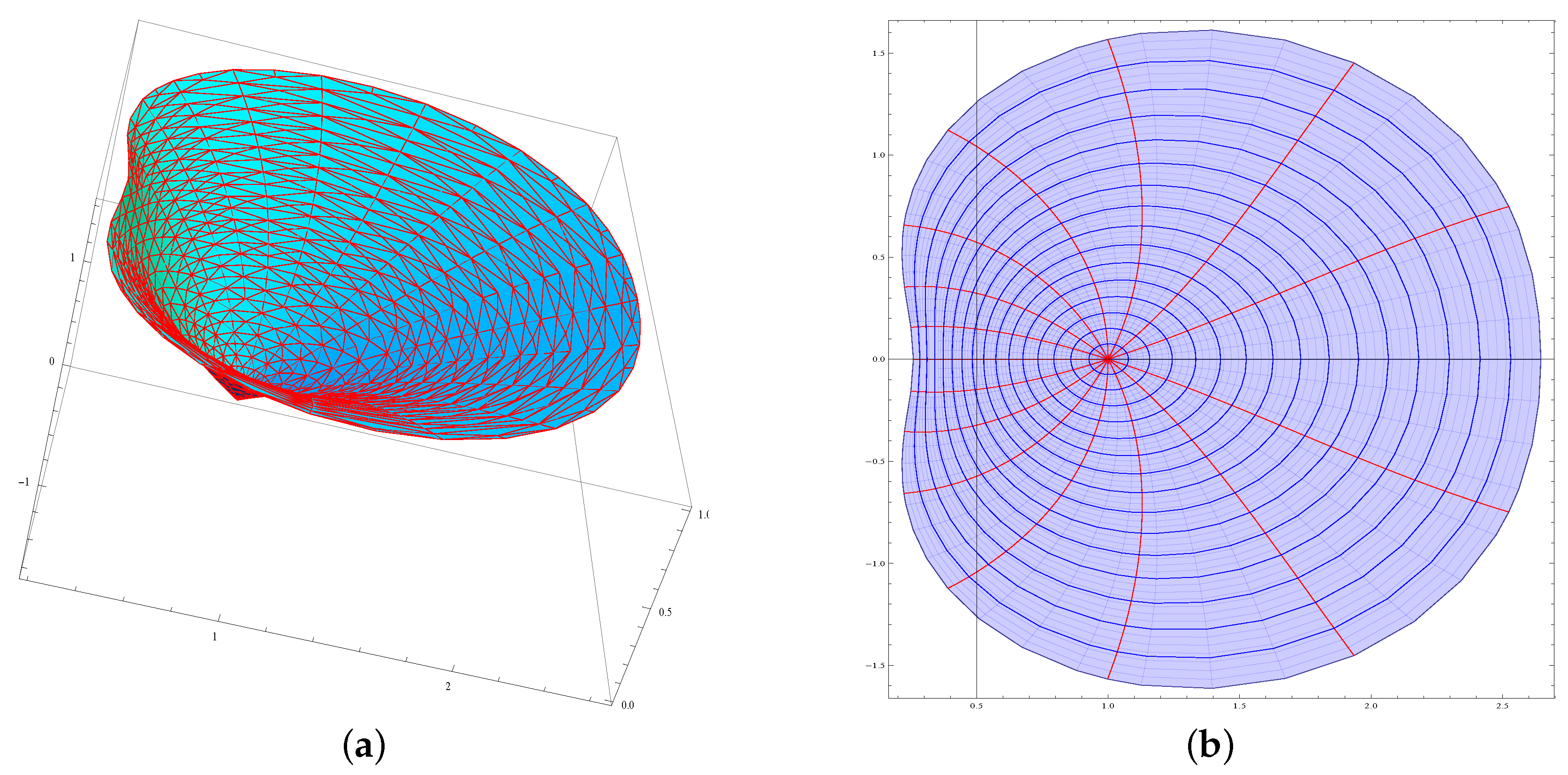
Example 1. The class is non-empty. Let , . Clearly, is univalent in and . Now,Wecan see that the function maps the unit disc onto a close to cardioid shaped region in the right-half plane (see Figure 1). Figure 1 shows the respective 3D view (Figure 1a) and 2D view (Figure 1b) of the mapping of unit disc under the mapping . Hence, . In the following example, we will show that functions which are starlike need not be in .
Example 2. Let , . The function is well known for mapping the unit disc onto a cardioid with cusp on the left-hand side. Further, the function is convex with respect to the point 1. Now,We can see that the function maps the unit disc onto a region as shown in Figure 2a. Figure 2a illustrates that does not belong to , even though , for ψ defined as in (8). Remark 2. Notice that is not a subclass nor a generalization of the class . For example, the function is in but does not belong to (see Figure 2b). Motivated by the definition of the operator (
6), Breaz et al. [
32] defined the following operator
by
Remark 3. Note that and . The operator includes many operators previously studied by various authors as its special cases. We list some of the special cases:
. The operator is the differential operator introduced and studied by Al-Oboudi [33]. , the operator is the well-known Sălăgean operator.
Obviously, fixing and in (9), then reduces to an operator defined and studied by Cang and Liu [27].
For a latest study of differential operators involving the Mittag–Leffler function, refer to Yassen and Attiya [34]. Motivated by the definition of , we now introduce and study a new class of analytic functions which is defined as follows.
Definition 1. Let denote the class of functions satisfying the conditionswhere , , and is defined as in (8). Remark 4. Here, we list some special cases of :
Letting , and in Definition 1, then the class reduces tothe class is the multiplicative analogue of the well-known class of starlike functions. Letting and in Definition 1, then the class given bythe class is a new class motivated by the relationship between starlike and convex function.
The does not have any well-known classes that describe it as a special case. Nonetheless, we will attempt to determine its connection to certain analytic function subclasses that have already been studied by other authors.
This paper is structured as follows. In
Section 3, we will obtain the coefficient bounds of
,
and solve the Fekete-Szegő problem for the defined function class
. Applications of our main results pertaining to vertical domain are presented as corollaries.
Section 4 is devoted to discuss the existence of an inverse function in the class
and obtain its coefficient estimates. Finally,
Section 5 has been devoted to present the bounds of logarithmic coefficients and their corresponding Fekete-Szegő functionals.
Now, we will state the following lemma, which we will use it to find the coefficient bounds.
Lemma 1 ([
35])
. If , and ρ is complex number, then and the result is sharp. 3. Initial Coefficients and Fekete-Szegő Inequality
We will begin the solution to the Fekete-Szegő problem for .
Theorem 1. If , then we haveand for all where is given byThe inequality is sharp for each . Proof. As
, by (
10) we have
Thus, let
be of the form
and defined by
On computation, the right-hand side of (
15)
The left-hand side of (
15) will be of the form
From (
17) and (
16), we obtain
and
Equation (
11) can be obtained by applying the well-known result of
in (
18). Applying Lemma 1 together with inequality
in (
12), we obtain (
12).
Now, to prove the Fekete-Szegő inequality for the class
, we consider
Using the triangle inequality and Lemma 1 in the above equality, we can obtain (
13). □
Let and in Theorem 1, we have the following.
Corollary 1. Let (see (7)). Then,and for a complex number ρ, Letting in Corollary 1, we get the following.
Corollary 2. Let satisfy the conditionThen,and for a complex number ρ, Remark 5. It is well-known that for , then for and the Fekete-Szegő for function in is known to be , and ρ is a complex number. In comparison with Corollary 2, we can conclude that the is neither a subclass nor generalization of the class .
Letting ( and are real numbers such that ) in Corollary 1, we get the following.
Corollary 3. Let satisfy the conditionThen,and for a complex number ρ, Proof. We note that the function
maps the open unit disk
onto a convex domain and is of the form
where
,
. We can obtain
and
Substituting the values of
and (
20) in Theorem 1, we obtain assertion of our corollary. □
4. Coefficient Estimates of
We let
to denote the class of functions univalent in
. It is well known from Koebe
-quarter theorem that every function
in
has an inverse
, defined by
and
, where
The functions in need not be univalent, but since for all and , there exists an inverse function in some small disk with a center at . Next, the result is valid only for the functions in which are univalent.
Theorem 2. Let and let be the inverse of φ defined bythenandwhere , is defined as in (14). Furthermore, for all where . The inequality is sharp for each . Proof. From
and (
21), we have
The estimate for
follows immediately from (
18). Letting
in (
13), we obtain the estimate
. To find the Fekete-Szegő inequality for the inverse function, consider
Changing
in (
13), we obtain the desired result. □
5. Logarithmic Coefficients for Functions Belonging to
Inspired by recent works like [
36,
37,
38], in this section we determine the coefficient bounds and Fekete-Szegő problem associated with the logarithmic function.
If the function
is analytic in
, such that
for all
, then the well-known logarithmic coefficients
,
, of
are given by
For a function
, the left-hand side of the subordination of Definition 1 should be an analytic function in
, hence
for all
. Therefore, for all functions
, the relation (
22) is well defined.
Theorem 3. If , with the logarithmic coefficients given by (22), thenwith For , we havewhere , is defined as in (14). Proof. From
and equating the first two coefficients of relation (
22), we get
Using (
18) and (
19), we obtain
Using (
11), it follows that
and fixing
in (
13), we get
where
is given by (
23). To find estimate (
24), consider
Changing
in (
13) and simplifying, we obtain the desired result. □
6. Conclusions
Under varying selections of the function and parameters in the Definition 1, the function class reduces to classes with good geometrical implications but not to well-known classes like spiral-like, starlike, and convex. So our main results have lots of applications; here, we restricted ourselves to pointing out only a few of them.
Given the fact that , computing the estimates involving long differential characterization, which is in the exponent of an exponential, is cumbersome. Hence, extending this study to the class of convex functions would be very complicated. Further, from the coefficient estimates (see Theorem 1), it is very clear that functions in are not univalent. Now, the question arises: what should be the radius of the disc so that functions in are univalent?
Author Contributions
Conceptualization, K.R.K. and G.M.; methodology, K.R.K. and G.M.; software, K.R.K. and G.M.; validation, K.R.K. and G.M.; formal analysis, K.R.K. and G.M.; investigation, K.R.K. and G.M.; resources, K.R.K. and G.M.; data curation, K.R.K. and G.M.; writing—original draft preparation, K.R.K. and G.M.; writing—review and editing, K.R.K. and G.M.; visualization, K.R.K. and G.M.; supervision, G.M.; project administration, G.M.; funding acquisition to pay for the APC. and K.R.K. All authors have read and agreed to the published version of the manuscript.
Funding
This research received no external funding.
Data Availability Statement
No new data were created or analyzed in this study.
Acknowledgments
Authors thank the Editor and all the reviewers for their helpful comments and suggestions, which helped us remove the mistakes and also led to improvement in the presentation of the results.
Conflicts of Interest
The authors declare no conflicts of interest.
References
- Cho, N.E.; Kumar, S.; Kumar, V.; Ravichandran, V. Radius problemsfor starlike functions associated with the sine function. Bull. Iran. Math. Soc. 2019, 45, 213–232. [Google Scholar] [CrossRef]
- Mendiratta, R.; Nagpal, S.; Ravichandran, V. On a subclass ofstrongly starlike functions associated with exponential functions. Bull. Malays. Math. Sci. Soc. 2015, 38, 365–386. [Google Scholar] [CrossRef]
- Sharma, K.; Jain, N.K.; Ravichandran, V. Starlike functionsassociated with cardioid. Afrika Math. 2016, 27, 923–939. [Google Scholar] [CrossRef]
- Wani, L.A.; Swaminathan, A. Starlike and convex functionsassociated with a Nephroid domain. Bull. Malays. Math. Sci. Soc. 2021, 44, 79–104. [Google Scholar] [CrossRef]
- Raina, R.K.; Sokól, J. On Coefficient estimates for acertain class of starlike functions. Hacettepe. J. Math. Statist. 2015, 44, 1427–1433. [Google Scholar] [CrossRef]
- Araci, S.; Karthikeyan, K.R.; Murugusundaramoorthy, G.; Khan, B. Φ-like analytic functions associated with a vertical domain. Math. Inequal. Appl. 2023, 26, 935–949. [Google Scholar] [CrossRef]
- Dziok, J.; Raina, R.K.; Sokół, J. On a class of starlike functions related to a shell-like curve connected with Fibonacci numbers. Math. Comput. Model. 2013, 57, 1203–1211. [Google Scholar] [CrossRef]
- Dziok, J.; Raina, R.K.; Sokół, J. On α-convex functions related to shell-like functions connected with Fibonacci numbers. Appl. Math. Comput. 2011, 218, 996–1002. [Google Scholar] [CrossRef]
- Dziok, J.; Raina, R.K.; Sokół, J. Certain results for a class of convex functions related to a shell-like curve connected with Fibonacci numbers. Comput. Math. Appl. 2011, 61, 2605–2613. [Google Scholar] [CrossRef]
- Gandhi, S.; Ravichandran, V. Starlike functions associated with a lune. Asian-Eur. J. Math. 2017, 10, 1750064. [Google Scholar] [CrossRef]
- Karthikeyan, K.R.; Murugusundaramoorthy, G. Unified solution of initial coefficients and Fekete–Szegö problem for subclasses of analytic functions related to a conic region. Afr. Mat. 2022, 33, 44. [Google Scholar] [CrossRef]
- Raina, R.K.; Sokół, J. Some properties related to a certain class of starlike functions. C. R. Math. Acad. Sci. Paris 2015, 353, 973–978. [Google Scholar] [CrossRef]
- Raina, R.K.; Sokół, J. Fekete-Szegö problem for some starlike functions related to shell-like curves. Math. Slovaca 2016, 66, 135–140. [Google Scholar] [CrossRef]
- Srivastava, H.M.; Ahmad, Q.Z.; Khan, N.; Khan, N.; Khan, B. Hankel and Toeplitz determinants for a subclass of q-starlike functions associated with a general conic domain. Mathematics 2019, 7, 181. [Google Scholar] [CrossRef]
- Srivastava, H.M.; Khan, B.; Khan, N.; Ahmad, Q.Z. Coefficient inequalities for q-starlike functions associated with the Janowski functions. Hokkaido Math. J. 2019, 48, 407–425. [Google Scholar] [CrossRef]
- Srivastava, H.M.; Raza, N.; AbuJarad, E.S.A.; Srivastava, G.; AbuJarad, M.H. Fekete-Szegö inequality for classes of (p, q)-starlike and (p,q)-convex functions. Rev. Real Acad. Cienc. Exactas Fís. Natur. Ser. A Mat. (RACSAM) 2019, 113, 3563–3584. [Google Scholar] [CrossRef]
- Srivastava, H.M.; Tahir, M.; Khan, B.; Ahmad, Q.Z.; Khan, N. Some general classes of q-starlike functions associated with the Janowski functions. Symmetry 2019, 11, 292. [Google Scholar] [CrossRef]
- Srivastava, H.M. An Introductory Overview of Special Functions and Their Associated Operators of Fractional Calculus. In Special Functions in Fractional Calculus and Engineering; Singh, H., Srivastava, H.M., Pandey, R.K., Eds.; CRC Press: Boca Raton, FL, USA, 2023; pp. 1–35. [Google Scholar]
- Srivastava, H.M. A survey of some recent developments on higher transcendental functions of analytic number theory and applied mathematics. Symmetry 2021, 13, 2294. [Google Scholar] [CrossRef]
- Srivastava, H.M. An introductory overview of fractional-calculus operators based upon the Fox-Wright and related higher transcendental functions. J. Adv. Engrg. Comput. 2021, 5, 135–166. [Google Scholar] [CrossRef]
- Srivastava, H.M. Some parametric and argument variations of the operators of fractional calculus and related special functions and integral transformations. J. Nonlinear Convex Anal. 2021, 22, 1501–1520. [Google Scholar]
- Srivastava, H.M.; Kumar, A.; Das, S.; Mehrez, K. Geometric properties of a certain class of Mittag–Leffler-type functions. Fractal Fract. 2022, 6, 54. [Google Scholar] [CrossRef]
- Srivastava, H.M.; Fernandez, A.; Baleanu, D. Some new fractional-calculus connections between Mittag–Leffler functions. Mathematics 2019, 7, 485. [Google Scholar] [CrossRef]
- Srivastava, H.M.; Bansal, M.; Harjule, P. A study of fractional integral operators involving a certain generalized multi-index Mittag–Leffler function. Math. Methods Appl. Sci. 2018, 41, 6108–6121. [Google Scholar] [CrossRef]
- Srivastava, H.M.; Tomovski, Ž. Fractional calculus with an integral operator containing a generalized Mittag–Leffler function in the kernel. Appl. Math. Comput. 2009, 211, 198–210. [Google Scholar] [CrossRef]
- Srivastava, H.M. On an extension of the Mittag–Leffler function. Yokohama Math. J. 1968, 16, 77–88. [Google Scholar]
- Cang, Y.-L.; Liu, J.-L. A family of multivalent analytic functions associated with Srivastava-Tomovski generalization of the Mittag–Leffler function. Filomat 2018, 32, 4619–4625. [Google Scholar] [CrossRef]
- Bashirov, A.E.; Kurpinar, E.M.; Özyapıcı, A. Multiplicative calculus and its applications. J. Math. Anal. Appl. 2008, 337, 36–48. [Google Scholar] [CrossRef]
- Bashirov, A.E.; Mısırlı, E.; Tandoğdu, Y.; Özyapıcı, A. On modeling with multiplicative differential equations. Appl. Math. J. Chin. Univ. 2011, 26, 425–438. [Google Scholar] [CrossRef]
- Bashirov, A.E.; Riza, M. On complex multiplicative differentiation. TWMS J. Appl. Eng. Math. 2011, 1, 75–85. [Google Scholar]
- Riza, M.; Özyapici, A.; Mısırlı, E. Multiplicative finite difference methods. Quart. Appl. Math. 2009, 67, 745–754. [Google Scholar] [CrossRef]
- Breaz, D.; Karthikeyan, K.R.; Umadevi, E.; Senguttuvan, A. Some properties of Bazilevič functions involving Srivastava-Tomovski operator. Axioms 2022, 11, 687. [Google Scholar] [CrossRef]
- Al-Oboudi, F.M. On univalent functions defined by a generalized Sălăgean operator. Int. J. Math. Math. Sci. 2004, 27, 1429–1436. [Google Scholar] [CrossRef]
- Yassen, M.F.; Attiya, A.A. Certain quantum operator related to generalized Mittag–Leffler function. Mathematics. 2023, 11, 4963. [Google Scholar] [CrossRef]
- Ma, W.C.; Minda, D. A unified treatment of some special classes of univalent functions. In Proceedings of the Conference on Complex Analysis at the Nankai Institue of Mathematics, Tianjin, China, 19–23 June 1992. [Google Scholar]
- Alimohammadi, D.; Cho, N.E.; Adegani, E.A.; Motamednezhad, A. Argument and coefficient estimates for certain analytic functions. Mathematics 2020, 8, 88. [Google Scholar] [CrossRef]
- Alimohammadi, D.; Analouei Adegani, E.; Bulboacă, T.; Cho, N.E. Logarithmic Coefficients for Classes Related to Convex Functions. Bull. Malays. Math. Sci. Soc. 2021, 44, 2659–2673. [Google Scholar] [CrossRef]
- Adegani, E.A.; Cho, N.E.; Jafari, M. Logarithmic coefficients for univalent functions defined by subordination. Mathematics 2019, 7, 408. [Google Scholar] [CrossRef]
| Disclaimer/Publisher’s Note: The statements, opinions and data contained in all publications are solely those of the individual author(s) and contributor(s) and not of MDPI and/or the editor(s). MDPI and/or the editor(s) disclaim responsibility for any injury to people or property resulting from any ideas, methods, instructions or products referred to in the content. |
© 2024 by the authors. Licensee MDPI, Basel, Switzerland. This article is an open access article distributed under the terms and conditions of the Creative Commons Attribution (CC BY) license (https://creativecommons.org/licenses/by/4.0/).


