Article

Diffusion of an Active Particle Bound to a Generalized Elastic Model: Fractional Langevin Equation

by
Alessandro Taloni
Istituto Sistemi Complessi, Consiglio Nazionale delle Ricerche, via dei Taurini 19, 00185 Rome, Italy
Fractal Fract. 2024, 8(2), 76; https://doi.org/10.3390/fractalfract8020076
Submission received: 23 November 2023 / Revised: 3 January 2024 / Accepted: 19 January 2024 / Published: 24 January 2024

Abstract

:
We investigate the influence of a self-propelling, out-of-equilibrium active particle on generalized elastic systems, including flexible and semi-flexible polymers, fluid membranes, and fluctuating interfaces, while accounting for long-ranged hydrodynamic effects. We derive the fractional Langevin equation governing the dynamics of the active particle, as well as that of any other passive particle (or probe) bound to the elastic system. This equation analytically demonstrates how the active particle dynamics is influenced by the interplay of both the non-equilibrium force and of the viscoelastic environment. Our study explores the diffusional behavior emerging for both the active particle and a distant probe. The active particle undergoes three different surprising and counter-intuitive regimes identified by the distinct dynamical time-scales: a pseudo-ballistic initial phase, a drastic decrease in the mobility, and an asymptotic subdiffusive regime.

1. Introduction

Active matter refers to a class of materials or systems whose individual components are active, meaning they can convert athermal energy from the environment or internal sources into directed motion or mechanical forces. These systems are characterized by the ability of their constituents to exhibit self-propelled motion, leading to collective behaviors and dynamic patterns that distinguish them from traditional equilibrium systems [1,2,3,4,5]. Thus, by definition, active systems violate the fluctuation–dissipation theorem (FDT) and encompass a wide range of phenomena observed in biological systems, such as swarming of birds [6,7,8,9,10,11] or schooling of fish [12,13,14], the run-and-tumble dynamics of micro swimmers [15,16,17,18,19], and the molecular motors-driven transport phenomena inside the cell [20,21,22,23]. Active matter can also originate synthetically, as seen in systems composed of Janus particles that become active due to chemical reactions [24,25], magnetic [26,27,28], or electrodynamical forces [29,30,31,32].
In the past decade, stochastic models have been devised to capture and reproduce observed out-of-equilibrium scenarios and their properties [33,34,35], as well as the resulting collective dynamics [29,36,37,38,39,40,41,41]. These models encompass run-and-tumble particle models [16,42,43], active Brownian particle (ABP) models [25,44,45], and active Ornstein–Uhlenbeck particle (AOUP) models [1,18,46,47,48,49,50].
Particular attention has been dedicated to the investigation of active polymer systems, specifically polymeric chains composed of active particles [51,52,53,54] or immersed in an active bath [50,53,55,56,57,58]. This interest has been partially motivated by the observed out-of-equilibrium intracellular transport and collective phenomena, where biopolymers and active elements coexist, as in the case of the chromatin inside the nucleus [59,60,61,62,63,64]; the acto-myosin [65,66,67,68,69,70,71], microtubule [72,73,74], or citoskeleton networks [75,76,77,78,79,80,81,82]; and mucin on the epithelial cell surfaces [83,84,85,86]. Usually, simulations of active polymers are enforced by either a self-propelling force tangential to the elastic chain [87,88,89,90,91], or by considering the monomers as active particles, thus resorting to the aforementioned models [52,53,92,93]. The phenomenology exhibited by active polymers is heterogeneous, ranging from translational [94,95] to reptation motion [88,89], swelling [52,53,96], looping [55], swirling [97], or shrinkage [98,99], according to the different parameters characterizing the active polymer model scrutinized.
As emphasized, the numerous numerical studies mentioned above primarily focus on active polymers or polymers embedded in a thermal bath. Nevertheless, three notable studies, both numerical and analytical, specifically investigate the impact of an active particle (or force) confined to a local portion of polymeric chains. In the works by Natali et al. [100] and Joo et al. [101], the dynamics of flexible (Rouse) polymers were examined with the addition of an active monomer, specifically an AOUP. In the first study [100], the head of the polymer was permitted to exhibit active non-equilibrium motion. In the second [101], the AOUP was positioned as the middle monomer, and the study extended to a flexible polymer network with the central cross-linker being the AOUP. The third study [102], conceptualized and conducted by part of the team from the second study, concentrated on investigating the impact of an AOUP on a semi-flexible polymer network. These works exhibit several common features: (i). they are primarily numerical studies, (ii) their analysis is rooted in discrete polymer models, and (iii) they reveal intriguing and non-trivial physical scenarios, both in the dynamics of the AOUP and in that of the other monomers. Particularly interesting are the transition from globule to elongated conformational dynamics observed in [100], the intermediate slowing down of the AOUP diffusional motion, in spite of the active self-propelling force, in [101,102], and the fact that the AOUP dynamics can be described by a fractional Langevin equation [103].
The analysis presented in this paper expands the scope of the applicability of the reported models. Specifically, we explore how an AOUP influences the thermal dynamics of a general viscoelastic system, whether it be a polymer, a membrane, a fluctuating interface, or any other system falling under the category of a generalized elastic model (GEM) [103,104]. The GEM is defined by its stochastic evolution equation:
t h x , t = d d x Λ x x C z x z h ( x , t ) + η x , t .
It is formally defined for D-dimensional stochastic field h defined in the d-dimensional infinite space x . The GEM also encompasses the presence of hydrodynamic effects, as in the case of a Zimm polymer model, by instance [105]. The hydrodynamic friction kernel is
Λ r = B γ r α
where d 1 2 < α < d , B is a constant with the dimensions of L α d and γ is the friction constant. The Fourier transform of (2) is Λ q = ( 4 π ) d / 2 2 α Γ ( d α ) / 2 Γ α / 2 B γ q α d = A q α d . In case of local hydrodynamic interactions, (2) simplifies to Λ r = δ ( r ) γ , with δ the Dirac’s delta function. The fractional derivative appearing in the right-hand side of (1) is commonly defined as fractional Laplacian ( z x z : = 2 z / 2 [106]), and is expressed in terms of its Fourier transform F q z x z q z [107]. Finally, the Gaussian random noise source satisfies the fluctuation–dissipation (FD) relation
η j x , t η k x , t = 2 k B T l d Λ x x δ j k δ ( t t ) ,
where j , k [ 1 , D ] , l is the microscopical length scale of the model, k B is the Boltzmann constant, and T is the temperature.
Although the GEM Equation (1) is continuous, it simplifies to the Rouse chain model for z = 2 , d = 1 , the semi-flexible polymer model for z = 4 , d = 1 , and the Zimm polymer model for z = 2 , d = 1 , and α = 1 / 2 . The influence of an active non-equilibrium particle on the elastic system described by (1) can be examined using the framework developed in [108,109,110], where the effect of a local external perturbation was investigated within the context of the Kubo fluctuation relations. It is worth noting that this analysis can be formally extended to the case of out-of-equilibrium stochastic forces.

Generalized Elastic Model with Active Brownian Particle

According to the theory outlined in [108,109,110], it is possible to include in the GEM stochastic evolution (1) the action of an ABP at a given position x :
t h x , t = d d x Λ x x C z x z h ( x , t ) + γ σ d γ A ξ ( t ) δ ( x x ) + η x , t .
Here, the active noise ξ ( t ) is due to an athermal energy source, leading to the breakdown of the FDT [18,33,111]. It is governed by the Langevin equation [52,111]
ξ t = ξ ( t ) τ A + 2 γ A ν p 3 τ A λ ( t )
where σ , γ A , ν p , and τ A are the characteristic length, the frictional coefficient, the propulsion velocity, and the correlation times of the Brownian active particle. The zero-mean Gaussian noise in Equation (5) satisfies the fluctuation–dissipation relation λ μ ( t ) λ ν ( t ) = δ μ , ν δ ( t t ) ( μ , ν [ 1 , D ] ). The Langevin Equation (5) rules the dynamics of the active Ornstein–Uhlenbeck (OU) noise [18,33,111] with ξ ( t ) = 0 and exponential decaying autocorrelation function
ξ μ ( t ) ξ ν ( t ) = γ 2 ν p 2 3 δ μ , ν e | t t | τ A .
Hence, hereafter, we will refer to the self-propelling particle at x as the AOUP. The Equation (4) jibes with that furnished in [101], provided that C = k l 2 , where k is the flexible polymer’s elastic constant. On the other side, the corresponding GEM equation for AOUP in a semi-flexible chain is obtained by setting Λ r = δ ( r ) γ , z = 4 , d = 1 [104]. It is possible to reconcile the evolution Equation (4) with that introduced in [102], assuming that C = k B T l p l , where l p is the persistent length of the semi-flexible polymer.
As anticipated, we demonstrate that Equation (4) constitutes the more general and suitable framework to study the effect of a self-propelling AOUP on a system whose interactions are non-local and linear, and possibly mediated by long-ranged hydrodynamics. In Section 2, we derive the fractional Langevin equation for the AOUP and for any particle belonging to the elastic system at a generic position x , hereafter called probe. In Section 3, we derive the position autocorrelation function within the FLE framework. In Section 4, we furnish the analytical derivation of the mean squared displacement of the AOUP and of the different regimes attained. Moreover, we qualitatively describe the effect of the OU noise on the other regions (or probes) belonging to the elastic system and far from the AOUP. In Section 5, we end with concluding remarks.

2. Fractional Langevin Equation

We firstly furnish the solution of the Equation (4) in the Fourier space. We first define the Fourier transform in space and time as
h q , ω = + d d x + d t h x , t e i q · x ω t
The solution of Equation (4) reads
h q , ω = A σ d γ γ A ξ ( ω ) e i q · x q d α i ω + A C q z + α d + η q , ω i ω + A C q z + α d .
We then multiply both sides of the former equation by K + ( i ω ) β where
β = z d z + α d
and
K + = π d / 2 1 sin π β Γ ( d / 2 ) 2 2 d ( z + α d ) A β C β 1 ,
achieving
K + ( i ω ) β h q , ω = σ d γ γ A ξ ( ω ) K + A ( i ω ) β e i q · x q d α i ω + A C q z + α d + η q , ω K + ( i ω ) β i ω + A C q z + α d .
In analogy to [108,109,110], we define the force-propagator in the Fourier space as
Θ q , ω = K + A ( i ω ) β e i q · x q d α i ω + A C q z + α d .
Inverting in space and time, the force-propagator reads [109,110]
Θ x x , t = A K + x 1 d / 2 ( 2 π ) d / 2 0 + d q q α d / 2 J d / 2 1 q x x D t β e A C q γ / 2 t θ ( t ) ,
where θ ( t ) is the Heaviside step function, J d / 2 1 is the Bessel function of fractional order d / 2 1 , and the pseudo-differential operator
D t β a ϕ ( t ) = 1 Γ 1 β d d t a t d t 1 t t β ϕ t , 0 < β < 1 ,
represents the left side Riemann–Liouville derivative with lower-bound a < t [106,112].
We also introduce the noise-propagator as
Φ q , ω = K + ( i ω ) β i ω + A C q z + α d ,
which, once inverted, attains the following form in space and time:
Φ x , t = A K + x 1 d / 2 ( 2 π ) d / 2 0 + d q q d / 2 J d / 2 1 q x D t β e A C q γ / 2 t θ ( t ) .
Thanks to the definitions (12) and (15), we can formally invert the Equation (11):
K + D t β h x , t = σ d γ γ A t d t ξ ( t ) Θ x x , t t + ζ x , t ,
where the non-Markovian noise, defined as
ζ x , t = + d x t d t η x , t Φ x x , t t ,
fulfills the generalized fluctuation–dissipation relation
ζ μ x , t ζ ν x , t = k B T δ μ , ν K + Γ 1 β t t β .
Equation (17) is the fractional equation governing the dynamics of any probe placed at the generic position x . Upon close inspection, its structure unveils how the action of the AOUP in the position x * affects the stochastic behavior of a distant point x , through the propagator (13). This is mirrored by the fGN definition (18), resulting from the convolution of any stochastic Gaussian force η x , t , performing on the entire GEM, with the noise-propagator (16). Notice that the Riemann–Liouville fractional derivative in (14) could be safely replaced by the Caputo fractional derivative in the FLE (17), as both definitions coincide when the lower bound tends to [106,112].
We now turn to the expression of the effective stochastic equation ruling out the motion of the AOUP. For such a purpose, we first perform the Fourier inverse transform in space of the expression (12):
Θ x x * , ω = A K + ( i ω ) β x 1 d / 2 ( 2 π ) d / 2 0 + d q q α d / 2 J d / 2 1 q x x * i ω + A C q z + α d ,
hence, we use the expansion of the Bessel function for small arguments as [113]
J d / 2 1 ( r ) 1 Γ ( d / 2 ) 2 r 1 d / 2 ,
obtaining
Θ 0 , ω A β K + 2 1 d / 2 ( 2 π ) d / 2 Γ d 2 C 1 β 0 + d y y α 1 1 + y z + α d .
Solving the integral [114], we finally obtain that
Θ 0 , ω 1 2 l d δ ( t t ) .
Therefore, Equation (17) reduces to the following fractional equation for the AOUP:
K + D t β h x * , t = σ d γ 2 l d γ A ξ ( t ) + ζ x * , t .
Thus, it is immediately seen how the active noise applies to the AOUP as a barestochastic force. Similar equations were conjectured in Refs. [101,102], while analyzing the case of flexible and semi-flexible polymers under the action of an ABP. We hereby offered the rigorous derivation in the more general case represented by the GEM (1). Moreover, we established the formal validity of the FLE framework for any particle, not only for the AOUP.
Most importantly, Equations (17) and (24) highlight how the motion of any probe in the elastic system, being the AOUP at x * or another at a position x , corresponds to a fractional Brownian motion [115].

3. h-Autocorrelation Function

The MSD of any particle belonging to the GEM is affected by the presence of the active noise ξ ( t ) . As a matter of fact, the general expression for the MSD reads
δ 2 h x , t h x , t h x , 0 2 = 2 h 2 x , t h x , t h x , 0
where h x , t represents one of the components of the stochastic field h x , t . From the definition (25), it turns out that the calculation of the MSD, as that of any other physical observable, needs the explicit expression of the two-times autocorrelation function h x , t h x , t .
Starting from the single component solution of the Equation (17) in the Fourier space
h x , ω = σ d γ γ A ξ ( ω ) Θ x x , ω K + ( i ω ) β + ζ x , ω K + ( i ω ) β ,
we can write down
h x , ω h x , ω = σ d γ γ A 2 x x 2 d 0 + d q q α d / 2 J d / 2 1 q x x * × 0 + d q q α d / 2 J d / 2 1 q x x * ξ ( ω ) ξ ( ω ) i ω + A C q z + α d i ω + A C q z + α d + ζ ( x , ω ) ζ ( x , ω ) K + 2 ( i ω ) β ( i ω ) β ,
where we made use of the force-propagator Fourier transform (20). The first addendum on the RHS of the previous equation can be further simplified by resorting to the active noise correlation properties in Fourier space, i.e.,
ξ ( ω ) ξ ( ω ) = 4 π ν p 2 γ A 2 3 τ A δ ( ω + ω ) 1 τ A 2 + ω 2 .
The second addendum is the usual term accounting for the correlations inherent to the GEM [104]. Therefore, the h-autocorrelation function obtains the final form
h x , t h x , t = ( σ d γ A ν p ) 2 x x 2 d 2 d 1 π d + 1 3 τ A × 0 + d q q α d / 2 J d / 2 1 q x x * 0 + d q q α d / 2 J d / 2 1 q x x * × d ω e i ω ( t t ) 1 τ A 2 + ω 2 i ω + A C q z + α d i ω + A C q z + α d + 2 2 d k B T l d A β C β 1 ( z + α d ) π d / 2 Γ d 2 cos π β 2 0 d ω cos [ ω ( t t ) ] ω 1 + β ,
The two terms appearing on the RHS of the autocorrelation function have a different origin and different behaviors. While in the first one it appears clear the dependence on the internal coordinate x as well as the absence of any divergence in the ω space, the second does not depend on the specific internal position but diverges as | ω | ( 1 + β ) in the limit of ω 0 [104]. Therefore, any physically measurable quantity must be organized in a manner that ensures the cancellation of this divergence.
The h-autocorrelation function of the AOUP is obtained from Equation (28) using the property (21)
h x * , t h x * , t = σ d γ ν p l d K + 2 1 6 π τ A 0 d ω cos [ ω ( t t ) ] ω 2 β 1 τ A 2 + ω 2 + 2 2 d k B T l d A β C β 1 ( z + α d ) π d / 2 Γ d 2 cos π β 2 0 d ω cos [ ω ( t t ) ] ω 1 + β
The same expression is achievable from the solution of Equation (24) in Fourier space:
h x * , ω = σ d γ 2 l d γ A ξ ( ω ) K + ( i ω ) β + ζ x * , ω K + ( i ω ) β ,

4. Mean Square Displacement

By substituting the expression (28) by the MSD definition (25), it becomes evident that the MSD is composed of the sum of two contributions:
δ 2 h x , t = δ 2 h x , t O U N + δ 2 h x , t f G N .
As noticed in Ref. [102], this superposition makes non-trivial the possible diffusive scenario arising when we are considering both the AOUP and a generic probe. We consider the case of high Péclet number where the active dynamics is definitely larger that the thermal counterpart. Indeed, the first in Equation (31) arises from the action of the non-equilibrium Ornstein–Uhlenbeck noise ruled by the Langevin equation (5), whereas the second stems from the fractional Gaussian noise (18) and represents the typical subdiffusive thermal dynamics exhibited by any element belonging to the GEM (1) [103,104]:
δ 2 h x , t f G N = 4 k B T π d / 2 ( A C ) β Γ ( 1 β ) ( 2 π ) d Γ ( d / 2 ) ( z d ) C t β
The first term on the RHS of (31) is formally defined as
δ 2 h x , t O U N = ( σ d γ A ν p ) 2 x x 2 d 2 d 1 π d + 1 3 τ A × 0 + d q q α d / 2 J d / 2 1 q x x * 0 + d q q α d / 2 J d / 2 1 q x x * × d ω 1 e i ω t 1 τ A 2 + ω 2 i ω + A C q z + α d i ω + A C q z + α d .
The equivalent term in case of the AOUP can be derived from (29)
δ 2 h x * , t O U N = σ d γ ν p l d K + 2 1 3 π τ A 0 d ω 1 cos ( ω t ) ω 2 β 1 τ A 2 + ω 2
and it is definitely easier to treat. Hence, in the following we develop our analysis starting from the expression (34).

4.1. AOUP’s MSD

Firstly, we notice how, in the integral
I = 0 d ω 1 cos ( ω t ) ω 2 β 1 τ A 2 + ω 2
there is no issue of divergence in the limit as ω 0 . In fact, the integrand function behaves as ω 2 ( 1 β ) for small frequencies. We then introduce a change in variable, y = ω τ A , so that
I = τ A 1 + 2 β 0 d y 1 cos y t τ A y 2 β 1 + y 2 .
Its time behavior differs whether t τ A or t τ A and we will treat them separately.

4.1.1. t τ A

The integral (35) must be handled differently in the three cases 0 < β < 1 / 2 , β = 1 / 2 , and 1 / 2 < β < 1 .
  • 0 < β < 1 / 2 .
    We can split the integral and solve the first one [114]:
    I = τ A 1 + 2 β π 2 c o s e c ( 1 2 β ) π 2 0 d y cos y t τ A y 2 β 1 + y 2 .
    Hence, we integrate the second by parts and we expand the resulting trigonometric functions for small arguments
    I = τ A 1 + 2 β π 2 c o s e c ( 1 2 β ) π 2 1 1 2 β t τ A 2 0 d y y 2 2 β 1 + y 2 0 d y y 3 2 β ( 1 + y 2 ) 2 + 2 0 d y y 2 2 β ( 1 + y 2 ) 2 .
    By evaluating the remaining integrals, we obtain the final result
    I = τ A 1 + 2 β π 2 t τ A 2 c o s e c ( 2 β 3 ) π 2 1 2 β + c o s e c ( 1 2 β ) π 2 2 + π c o s e c ( 1 2 β ) π 2 2 β c o s e c π β 1 2 β .
  • β = 1 / 2 .
    The integral (35) is in this case
    I = τ A 2 0 d y 1 cos y t τ A y 1 + y 2 .
    Integrating by parts, we have
    I = τ A 2 t τ A 0 ln ( y ) sin y t τ A 1 + y 2 + 2 0 d y ln ( y ) 1 cos y t τ A ( 1 + y 2 ) 2 .
    We can neglect the second and split the first into two contributions
    I = τ A 2 t τ A 0 1 ln ( y ) sin y t τ A 1 + y 2 + t τ A 1 ln ( y ) sin y t τ A 1 + y 2 .
    Then, we can retain only the first one, as the second is nearly zero, and expand the sine for small arguments, obtaining [114]
    I = τ A 2 t τ A 2 0 1 y ln ( y ) 1 + y 2 = t 2 π 2 48 .
  • 1 / 2 < β < 1 .
    This case is the easier to be handled. Expanding the cosine for small arguments in (35) yields
    I = t 2 τ A 1 2 β 1 2 0 d y y 2 ( 1 β ) 1 + y 2 = t 2 τ A 1 2 β π 4 c o s e c ( 3 2 β ) π 2

4.1.2. t τ A

This time limit presents the same symmetry of the previous one; therefore, we study the behavior of I in the three cases 0 < β < 1 / 2 , β = 1 / 2 , and 1 / 2 < β < 1 .
  • 0 < β < 1 / 2 .
    From (36), after integrating by parts, it is obtained
    I = τ A 1 + 2 β π 2 c o s e c ( 1 2 β ) π 2 t τ A 1 1 2 β 0 d y sin y t τ A y 2 β 1 1 + y 2 2 1 2 β 0 d y cos y t τ A y 2 β 2 1 + y 2 .
    The major contributions to the integrals appearing in (44) come from y 0 ; hence, I may be properly approximated to
    I = τ A 1 + 2 β π 2 c o s e c ( 1 2 β ) π 2 t τ A 1 1 2 β 0 d y y 1 2 β sin y t τ A 2 1 2 β 0 d y y 2 2 β cos y t τ A .
    We can thus use the method of summation of improper integrals [108,116] to finalize the calculation
    I = τ A 1 + 2 β π 2 c o s e c ( 1 2 β ) π 2 t τ A 2 β 1 Γ ( 2 2 β ) sin [ π ( 1 β ) ] 1 2 β t τ A 2 β 3 Γ ( 3 2 β ) cos π ( 3 2 β ) 2 1 2 β .
  • β = 1 / 2 .
    We recap from the expression (40), neglecting the second integral on the RHS and retaining only the contributions coming from y 0 in the first:
    I = τ A 2 t τ A 0 ln ( y ) sin y t τ A .
    Then, we can split the resulting integral into two terms
    I = τ A 2 t τ A 0 1 ln ( y ) sin y t τ A + t τ A 1 ln ( y ) sin y t τ A .
    and consider only the first one as the second yields almost no contribution. Finally, solving the integral [114],
    I = τ A 2 γ + ln t τ A C i t τ A ,
    where γ is the Euler–Mascheroni constant and C i is the cosine integral [113].
  • 1 / 2 < β < 1 .
    As in the previous situations, the main contributions to the integral in (35) will arise from y 0 ; hence,
    I = τ A 1 + 2 β 0 d y 1 cos y t τ A y 2 β .
    By integration by parts, it becomes
    I = τ A 1 + 2 β 2 β 1 t τ A 0 d y y 1 2 β sin y t τ A
    and, using the methods of improper integrals [116], the final result is
    I = τ A 1 + 2 β t τ A 2 β 1 Γ ( 2 2 β ) 2 β 1 sin π ( 1 β )
Now, collecting the expressions achieved in these subsections, we can wrap them up in a unique compact formula:
when
t τ A :
δ 2 h x * , t O U N σ d γ ν p l d K + 2 t 2 3 π τ A τ A 2 β 1 π 2 c o s e c ( 2 β 3 ) π 2 1 2 β + c o s e c ( 1 2 β ) π 2 2 0 < β < 1 / 2 π 2 48 β = 1 / 2 τ A 2 β 1 π 4 c o s e c ( 3 2 β ) π 2 1 / 2 < β < 1 ;
when t τ A :
δ 2 h x * , t O U N σ d γ ν p l d K + 2 1 3 π τ A τ A 1 + 2 β π 2 c o s e c ( 1 2 β ) π 2 0 < β < 1 / 2 τ A 2 ln t τ A β = 1 / 2 t 2 β 1 τ A 2 Γ ( 2 2 β ) 2 β 1 sin π ( 1 β ) 1 / 2 < β < 1 ;
Hence, we can infer that the impact of the OUN on the AOUP diffusive dynamics exhibits pseudo-ballistic behavior for time intervals shorter than the active decorrelation time ( τ A ). However, this impact varies depending on whether β is less than, equal to, or greater than 1/2. This result must be summed to the contribution arising from the fGN according to the formula (31). It is clear that, in the long time limit, the term δ 2 h x * , t f G N will dominate. However, the transition from the dynamics dictated by δ 2 h x * , t O U N to the asymptotic one will depend on the values of the parameters appearing in (4). Defining this transition time as τ s u b and assuming τ s u b τ A , a rough estimate of τ s u b could be given by equating the contributions of the expression (54) with (32): δ 2 h x * , τ s u b O U N = δ 2 h x * , τ s u b f G N . This is schematically shown in Figure 1.
However, it is essential to emphasize that, when we relax the assumption of τ sub τ A , the dynamics become less straightforward. Although the asymptotic behavior remains unchanged, the intermediate ultra-slow dynamics can be significantly compressed or reduced.

4.2. MSD at a Generic Position
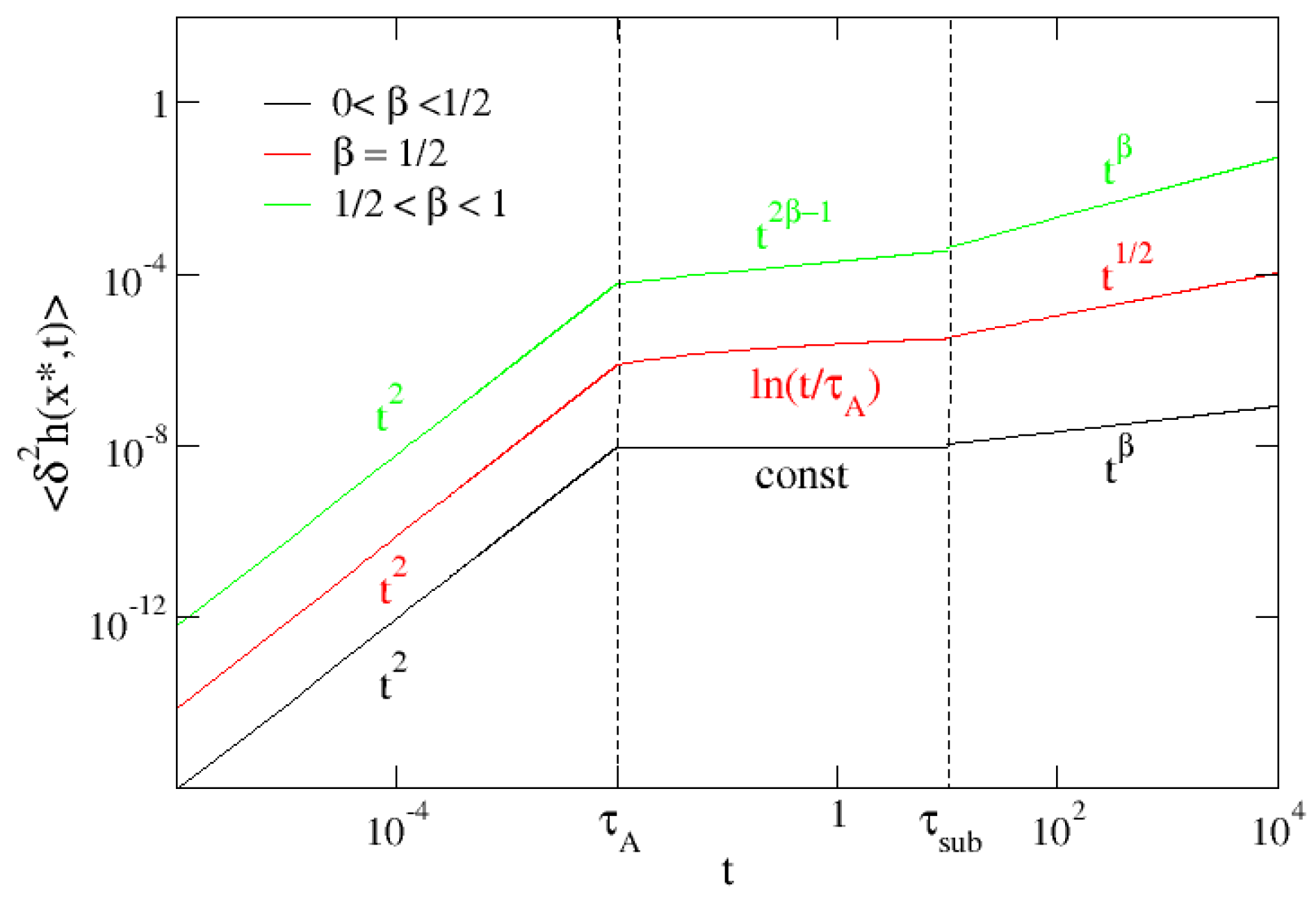
 x

The expression (33) is not straightforward to manipulate, making it challenging to deduce the impact of the AOUP dynamics on a tracer positioned at a distance of | x x * | . The reason is the appearance of a correlation time
τ ( | x x * | ) = | x x * | z + α d C A ,
which can be seen as the time up to which the dynamics of two distinct probes in x and x * is uncorrelated [108,109,110,117]. As a matter of fact, both the force- and the noise-correlators are expressed as Θ t τ ( | x | ) and Φ t τ ( | x | ) . The dependence of (31) and, in particular, the dependence of the δ 2 h ( x , t ) on the correlation time (55) can be achieved by the following changes in variable in the integrals of (33): y = C A i ω 1 / ( z + α d ) | q | , y = C A i ω 1 / ( z + α d ) | q | and λ = ω t :
δ 2 h x , t O U N = ( σ d γ A ν p ) 2 2 d 1 π d + 1 3 τ A x x α ( C A ) α z + α d t τ ( x x ) 2 + α d z + α d d λ 1 e i λ 1 τ A 2 + λ t 2 × 0 + d y y α d / 2 1 + y z + α d J d / 2 1 i λ τ ( x x ) t 1 z + α d y × 0 + d y y α d / 2 1 + y z + α d J d / 2 1 i λ τ ( x x ) t 1 z + α d y .
As previously mentioned, the formal analysis of (33) is not straightforward, and it will be the focus of an upcoming investigation. Nonetheless, we can qualitatively examine the limiting behaviors of the equivalent expression (56).
In the regime where t τ ( | x x * | ) , the Bessel functions exhibit high oscillations. As a result, the major contributions to the integrals come from values where y 0 , y 0 , and λ 0 . Surprisingly, these contributions are almost negligible, leading to
δ 2 h x , t δ 2 h x , t f G N .
In the opposite limit, where t τ ( | x x * | ) , we can employ the expansion of the Bessel functions for small arguments (21). This results in the same expression (34) as that valid for the AOUP. Consequently, we obtain
δ 2 h x , t δ 2 h x * , t O U N + δ 2 h x * , t f G N .
Given these limiting situations, we can provide an approximate study of the possible scenarios:
  • τ ( | x x * | ) τ A .
    Probes very close to the AOUP exhibit an initial thermal subdiffusive behavior t β . Subsequently, the probe at x behaves identically to the AOUP.
  • τ A τ ( | x x * | ) τ s u b .
    In this case, the probe’s diffusion is primarily governed by thermal noise. The non-equilibrium dynamics becomes significant only for τ ( | x x * | ) t τ s u b , leading to the results in (54). For longer times, i.e., t τ s u b , the thermal MSD (32) is recovered.
  • τ s u b τ ( | x x * | ) .
    Probes that satisfy this condition, i.e., probes far away from the AOUP, are not influenced by the action of the active force.

5. Concluding Remarks

In this paper, we examined the diffusional dynamics of an AOUP connected to an elastic system such as a (semi)flexible polymer, a membrane, or a fluctuating interface, including hydrodynamic fluid-mediated interactions. Moreover, we investigated the action of the non-equilibrium OU force on the other element belonging to the elastic system. We have demonstrated that the FLE constitutes the correct description of the AOUP dynamics, where the thermal contributions deriving from the rest of the elastic system are incorporated into the fGN, in addition to a renormalized OUN (24). We also derived the FLE for any other probe placed at an arbitrary distance from the AOUP | x x * | . Here, the effect of the non-equilibrium force is delayed in time, propagating through the medium thanks to the force-propagator Θ ( | x x * | , t ) (17).
Our analytical theory constitutes a significant improvement over the arguments presented in previous works on this subject. In Ref. [101], the FLE for the AOUP was inferred from the numerical evidence of the velocity autocorrelation function’s time behavior and from that of the MSD. In other words, it was proposed as an effective equation supported by analytical calculations drawn from a normal mode expansion [87,118,119,120]. However, a formal derivation of the FLE, based on the analysis by Panja [121,122], was not attempted.
In Ref. [102], the mesoscopic FLE for the AOUP attached to a (semi)flexible chain was introduced to reproduce its stochastic non-equilibrium dynamics. The fractional equation, namely the damping kernel, was derived by resorting to the tension propagation theory in the absence of active noise. However, even in this case, a formal derivation from the semi-flexible evolution equation was not provided.
In this article, we offered such an analytical derivation, significantly expanding the domain of its applicability to any elastic system, including hydrodynamics. This became possible because the framework of the FLE with a localized applied potential [108] could be entirely shifted to the case of the AOUP particle bound to an elastic system. Moreover, this framework entails the derivation of the FLE for any other probe belonging to the GEM, different from the AOUP.
The FLE framework provides a crucial additional value through the formally easy calculation of any observable composed as a function of the elementary correlation function (28). In particular, we examined the MSD of AOUP, uncovering some unexpected diffusional scenarios, which include, as special cases, those found in the simulations and theoretical analyses of Refs. [101,102].
Firstly, we observed how three different types of diffusion arise depending on the value of β . This is not immediately apparent in the early time regime, i.e., t τ A , when the action of the non-equilibrium OU noise drives the directional motion of the AOUP. In this regime, a super-diffusive pseudo-ballistic dynamics emerges, analogous to the result in [101] where the Rouse model yields β = 1 / 2 [103,104]. However, although the ∼ t 2 behavior is maintained for any value of β , the prefactors change significantly, as shown in Equation (53). Moreover, we observe that the ballistic regime may not distinctly emerge from simulations. Specifically, at low Péclet numbers, the contribution to the MSD from the thermal part, attributed to the action of the fractional Gaussian noise in (31), cannot be entirely neglected. This observation may underlie the ∼ t 3 / 2 behavior exhibited by the AOUP connected to semi-flexible polymers [102]. Simultaneously, this discrepancy could be attributed to the fact that, in the presented simulation results, the AOUP was attached to a network of four semi-flexible arms. Regardless, as highlighted by the same authors, in the simulations, “the superdiffusion for t τ A occurs with an anomalous exponent slightly greater than 3/2”.
For times t τ A and for high Péclet numbers, the diffusion is still dictated by the non-equilibrium active force, and the diffusional scenarios are different according to the values of β , as seen in Equation (54). For example, we both recover the logarithmic dependence of the Rouse chains, obtained analytically in [101], and the t 1 / 2 behavior observed in the numerical simulations of Ref. [102]. In the case of the Zimm polymers model instead, we predict ∼ t 1 / 3 in this regime, being β = 2 3 . Importantly, we anticipate that for β in the range 0 < β < 1 / 2 , the diffusion tends to slow down until reaching a constant value, as seen in Equation (54).
The asymptotic diffusion requires special attention. The FLEs (17) and (24) involve the superposition of both non-equilibrium and thermal contributions, resulting in the expression (31). This implies that, for a high Péclet number, there is a crossover between the active subdiffusive motion and the long-time thermal subdiffusive dynamics. The time scale on which this crossover occurs, denoted as τ s u b , is not easily determined and crucially depends on the microscopic parameters of the model, as illustrated in Figure 1. Situations may arise in which τ s u b τ A , causing the contribution in (54) to become less apparent. For the sake of clarity in our analysis, we focus on cases where τ s u b τ A .
The transition to thermal motion was also observed in the analysis presented in Refs. [101,102]. This crossover time was defined as τ R , signifying Rouse’s time in [101] and the relaxation time in the case of semi-flexible chains [102]. Both interpretations could be seen as thresholds marking the transition to the Brownian linear regime.As we are working with infinite systems, τ R in our context. Consequently, as the influence of the non-equilibrium OU active drive diminishes ( t τ A ), the thermal dynamics predominates ( t τ s u b ).
The analysis of the MSD of probes other than AOUP is complex and will be addressed elsewhere. However, even without a detailed analytical derivation, some important conclusions can be drawn. As discussed in Section 4.2, the dynamics of regions in the elastic system close to the AOUP are primarily influenced by the active non-equilibrium force up to τ s u b , with an initial thermal subdiffusive motion. For t τ s u b , the MSD of the probes is still governed by fractional Gaussian noise (fGN).
The initial thermal regime becomes more pronounced as one considers regions progressively farther from the AOUP. Consequently, the non-equilibrium component of the MSD, denoted as δ 2 h x , t O U N , diminishes. In the limit of very distant regions satisfying τ ( | x x | ) τ s u b , the diffusion of the probes is entirely dictated by thermal fluctuations, rendering the impact of any non-equilibrium driving force negligible. It is worth highlighting that this diffusional scenario precisely aligns with the findings from the numerical simulations in Ref. [101].
The numerical implementation of GEM with an active particle can be pursued by the numerical integration of the entire system governing Equation (4). Alternatively, one could just simulate the AOUP FLE (24) or the distant probe FLE (17). As stated in [103], both descriptions offer the same level of complexity, although the FLE framework provides a simpler and faster way to delve into the dynamical regimes of a single particle. Furthermore, the universal nature of the FLE equation allows for the definition of universality classes, categorized by the value of β . The most effective method to simulate the FLE is to utilize the ( k , ω ) solution, as given in Equation (11), and then invert it. Overall, these results may help to elucidate in vivo dynamics observed in experiments [63,76].

Funding

This research received no external funding.

Data Availability Statement

This study did not report any data.

Conflicts of Interest

The authors declare no conflict of interest.

References

  1. Bechinger, C.; Di Leonardo, R.; Löwen, H.; Reichhardt, C.; Volpe, G.; Volpe, G. Active particles in complex and crowded environments. Rev. Mod. Phys. 2016, 88, 45006. [Google Scholar] [CrossRef]
  2. Marchetti, M.C.; Joanny, J.F.; Ramaswamy, S.; Liverpool, T.B.; Prost, J.; Rao, M.; Simha, R.A. Hydrodynamics of soft active matter. Rev. Mod. Phys. 2013, 85, 1143. [Google Scholar] [CrossRef]
  3. Elgeti, J.; Winkler, R.G.; Gompper, G. Physics of microswimmers—Single particle motion and collective behavior: A review. Rep. Prog. Phys. 2015, 78, 56601. [Google Scholar] [CrossRef]
  4. Romanczuk, P.; Bär, M.; Ebeling, W.; Lindner, B.; Schimansky-Geier, L. Active Brownian particles: From individual to collective stochastic dynamics. Eur. Phys. J. Spec. Top. 2012, 202, 1–162. [Google Scholar] [CrossRef]
  5. Ramaswamy, S. The mechanics and statistics of active matter. Annu. Rev. Condens. Matter Phys. 2010, 1, 323–345. [Google Scholar] [CrossRef]
  6. Reynolds, C.W. Flocks, herds and schools: A distributed behavioral model. In Proceedings of the 14th Annual Conference on Computer Graphics and Interactive Techniques, Anaheim, CA, USA, 27–31 July 1987; pp. 25–34. [Google Scholar]
  7. Olfati-Saber, R. Flocking for multi-agent dynamic systems: Algorithms and theory. IEEE Trans. Autom. Control. 2006, 51, 401–420. [Google Scholar] [CrossRef]
  8. Czirók, A.; Barabási, A.L.; Vicsek, T. Collective motion of self-propelled particles: Kinetic phase transition in one dimension. Phys. Rev. Lett. 1999, 82, 209. [Google Scholar] [CrossRef]
  9. Bialek, W.; Cavagna, A.; Giardina, I.; Mora, T.; Silvestri, E.; Viale, M.; Walczak, A.M. Statistical mechanics for natural flocks of birds. Proc. Natl. Acad. Sci. USA 2012, 109, 4786–4791. [Google Scholar] [CrossRef]
  10. Cavagna, A.; Cimarelli, A.; Giardina, I.; Parisi, G.; Santagati, R.; Stefanini, F.; Viale, M. Scale-free correlations in starling flocks. Proc. Natl. Acad. Sci. USA 2010, 107, 11865–11870. [Google Scholar] [CrossRef]
  11. Attanasi, A.; Cavagna, A.; Del Castello, L.; Giardina, I.; Grigera, T.S.; Jelić, A.; Melillo, S.; Parisi, L.; Pohl, O.; Shen, E.; et al. Information transfer and behavioural inertia in starling flocks. Nat. Phys. 2014, 10, 691–696. [Google Scholar] [CrossRef]
  12. Couzin, I.D.; Ioannou, C.C.; Demirel, G.; Gross, T.; Torney, C.J.; Hartnett, A.; Conradt, L.; Levin, S.A.; Leonard, N.E. Uninformed individuals promote democratic consensus in animal groups. Science 2011, 334, 1578–1580. [Google Scholar] [CrossRef] [PubMed]
  13. Pérez-Escudero, A.; de Polavieja, G. Collective animal behavior from Bayesian estimation and probability matching. PLoS Comput. Biol. 2011, 7, e1002282. [Google Scholar]
  14. Couzin, I.D.; Krause, J. Self-organization and collective behavior in vertebrates. Adv. Study Behav. 2003, 32, 10–1016. [Google Scholar]
  15. Berg, H.C. E. coli in Motion; Springer: Berlin/Heidelberg, Germany, 2004. [Google Scholar]
  16. Lauga, E.; Goldstein, R.E. Dance of the microswimmers. Phys. Today 2012, 65, 30–35. [Google Scholar] [CrossRef]
  17. Matthäus, F.; Jagodič, M.; Dobnikar, J. E. coli superdiffusion and chemotaxis—Search strategy, precision, and motility. Biophys. J. 2009, 97, 946–957. [Google Scholar] [CrossRef] [PubMed]
  18. Wu, X.L.; Libchaber, A. Particle diffusion in a quasi-two-dimensional bacterial bath. Phys. Rev. Lett. 2000, 84, 3017. [Google Scholar] [CrossRef] [PubMed]
  19. Leptos, K.C.; Guasto, J.S.; Gollub, J.P.; Pesci, A.I.; Goldstein, R.E. Dynamics of enhanced tracer diffusion in suspensions of swimming eukaryotic microorganisms. Phys. Rev. Lett. 2009, 103, 198103. [Google Scholar] [CrossRef]
  20. Gal, N.; Weihs, D. Experimental evidence of strong anomalous diffusion in living cells. Phys. Rev. E 2010, 81, 20903. [Google Scholar] [CrossRef]
  21. Chen, K.; Wang, B.; Granick, S. Memoryless self-reinforcing directionality in endosomal active transport within living cells. Nat. Mater. 2015, 14, 589–593. [Google Scholar] [CrossRef]
  22. Gal, N.; Lechtman-Goldstein, D.; Weihs, D. Particle tracking in living cells: A review of the mean square displacement method and beyond. Rheol. Acta 2013, 52, 425–443. [Google Scholar] [CrossRef]
  23. Weber, C.A.; Suzuki, R.; Schaller, V.; Aranson, I.S.; Bausch, A.R.; Frey, E. Random bursts determine dynamics of active filaments. Proc. Natl. Acad. Sci. USA 2015, 112, 10703–10707. [Google Scholar] [CrossRef] [PubMed]
  24. Palacci, J.; Cottin-Bizonne, C.; Ybert, C.; Bocquet, L. Sedimentation and effective temperature of active colloidal suspensions. Phys. Rev. Lett. 2010, 105, 88304. [Google Scholar] [CrossRef] [PubMed]
  25. Howse, J.R.; Jones, R.A.; Ryan, A.J.; Gough, T.; Vafabakhsh, R.; Golestanian, R. Self-motile colloidal particles: From directed propulsion to random walk. Phys. Rev. Lett. 2007, 99, 48102. [Google Scholar] [CrossRef]
  26. Dreyfus, R.; Baudry, J.; Roper, M.L.; Fermigier, M.; Stone, H.A.; Bibette, J. Microscopic artificial swimmers. Nature 2005, 437, 862–865. [Google Scholar] [CrossRef] [PubMed]
  27. Tierno, P.; Golestanian, R.; Pagonabarraga, I.; Sagués, F. Controlled swimming in confined fluids of magnetically actuated colloidal rotors. Phys. Rev. Lett. 2008, 101, 218304. [Google Scholar] [CrossRef] [PubMed]
  28. Ghosh, A.; Fischer, P. Controlled propulsion of artificial magnetic nanostructured propellers. Nano Lett. 2009, 9, 2243–2245. [Google Scholar] [CrossRef]
  29. Bricard, A.; Caussin, J.B.; Desreumaux, N.; Dauchot, O.; Bartolo, D. Emergence of macroscopic directed motion in populations of motile colloids. Nature 2013, 503, 95–98. [Google Scholar] [CrossRef]
  30. Di Leonardo, R. Controlled collective motions. Nat. Mater. 2016, 15, 1057–1058. [Google Scholar] [CrossRef]
  31. Yan, J.; Han, M.; Zhang, J.; Xu, C.; Luijten, E.; Granick, S. Reconfiguring active particles by electrostatic imbalance. Nat. Mater. 2016, 15, 1095–1099. [Google Scholar] [CrossRef]
  32. Nishiguchi, D.; Iwasawa, J.; Jiang, H.R.; Sano, M. Flagellar dynamics of chains of active Janus particles fueled by an AC electric field. New J. Phys. 2018, 20, 15002. [Google Scholar] [CrossRef]
  33. Maggi, C.; Paoluzzi, M.; Angelani, L.; Di Leonardo, R. Memory-less response and violation of the fluctuation-dissipation theorem in colloids suspended in an active bath. Sci. Rep. 2017, 7, 17588. [Google Scholar] [CrossRef] [PubMed]
  34. Fodor, É.; Nardini, C.; Cates, M.E.; Tailleur, J.; Visco, P.; Van Wijland, F. How far from equilibrium is active matter? Phys. Rev. Lett. 2016, 117, 38103. [Google Scholar] [CrossRef]
  35. Maggi, C.; Paoluzzi, M.; Pellicciotta, N.; Lepore, A.; Angelani, L.; Di Leonardo, R. Generalized energy equipartition in harmonic oscillators driven by active baths. Phys. Rev. Lett. 2014, 113, 238303. [Google Scholar] [CrossRef]
  36. Cates, M.E.; Tailleur, J. Motility-induced phase separation. Annu. Rev. Condens. Matter Phys. 2015, 6, 219–244. [Google Scholar] [CrossRef]
  37. Reverey, J.F.; Jeon, J.H.; Bao, H.; Leippe, M.; Metzler, R.; Selhuber-Unkel, C. Superdiffusion dominates intracellular particle motion in the supercrowded cytoplasm of pathogenic Acanthamoeba castellanii. Sci. Rep. 2015, 5, 11690. [Google Scholar] [CrossRef] [PubMed]
  38. Budrene, E.O.; Berg, H.C. Dynamics of formation of symmetrical patterns by chemotactic bacteria. Nature 1995, 376, 49–53. [Google Scholar] [CrossRef]
  39. Brenner, M.P.; Levitov, L.S.; Budrene, E.O. Physical mechanisms for chemotactic pattern formation by bacteria. Biophys. J. 1998, 74, 1677–1693. [Google Scholar] [CrossRef]
  40. Omar, A.K.; Klymko, K.; GrandPre, T.; Geissler, P.L. Phase diagram of active Brownian spheres: Crystallization and the metastability of motility-induced phase separation. Phys. Rev. Lett. 2021, 126, 188002. [Google Scholar] [CrossRef]
  41. Alert, R.; Casademunt, J.; Joanny, J.F. Active turbulence. Annu. Rev. Condens. Matter Phys. 2022, 13, 143–170. [Google Scholar] [CrossRef]
  42. Kafri, Y.; da Silveira, R.A. Steady-state chemotaxis in Escherichia coli. Phys. Rev. Lett. 2008, 100, 238101. [Google Scholar] [CrossRef]
  43. Tailleur, J.; Cates, M. Statistical mechanics of interacting run-and-tumble bacteria. Phys. Rev. Lett. 2008, 100, 218103. [Google Scholar] [CrossRef] [PubMed]
  44. Ben-Isaac, E.; Fodor, É.; Visco, P.; Van Wijland, F.; Gov, N.S. Modeling the dynamics of a tracer particle in an elastic active gel. Phys. Rev. E 2015, 92, 12716. [Google Scholar] [CrossRef]
  45. Zheng, X.; Ten Hagen, B.; Kaiser, A.; Wu, M.; Cui, H.; Silber-Li, Z.; Löwen, H. Non-Gaussian statistics for the motion of self-propelled Janus particles: Experiment versus theory. Phys. Rev. E 2013, 88, 32304. [Google Scholar] [CrossRef] [PubMed]
  46. Nguyen, G.P.; Wittmann, R.; Löwen, H. Active Ornstein–Uhlenbeck model for self-propelled particles with inertia. J. Phys. Condens. Matter 2021, 34, 35101. [Google Scholar] [CrossRef] [PubMed]
  47. Caprini, L.; Marconi, U.M.B.; Wittmann, R.; Löwen, H. Dynamics of active particles with space-dependent swim velocity. Soft Matter 2022, 18, 1412–1422. [Google Scholar] [CrossRef]
  48. Sprenger, A.R.; Caprini, L.; Löwen, H.; Wittmann, R. Dynamics of active particles with translational and rotational inertia. J. Phys. Condens. Matter 2023, 35, 305101. [Google Scholar] [CrossRef] [PubMed]
  49. Caprini, L.; Bettolo Marconi, U.M.; Wittmann, R.; Löwen, H. Active particles driven by competing spatially dependent self-propulsion and external force. SciPost Phys. 2022, 13, 065. [Google Scholar] [CrossRef]
  50. Samanta, N.; Chakrabarti, R. Chain reconfiguration in active noise. J. Phys. Math. Theor. 2016, 49, 195601. [Google Scholar] [CrossRef]
  51. MacKintosh, F.C.; Janmey, P.A. Actin gels. Curr. Opin. Solid State Mater. Sci. 1997, 2, 350–357. [Google Scholar] [CrossRef]
  52. Eisenstecken, T.; Gompper, G.; Winkler, R.G. Conformational properties of active semiflexible polymers. Polymers 2016, 8, 304. [Google Scholar] [CrossRef]
  53. Kaiser, A.; Babel, S.; ten Hagen, B.; von Ferber, C.; Löwen, H. How does a flexible chain of active particles swell? J. Chem. Phys. 2015, 142, 124905. [Google Scholar] [CrossRef] [PubMed]
  54. Anand, S.K.; Singh, S.P. Behavior of active filaments near solid-boundary under linear shear flow. Soft Matter 2019, 15, 4008–4018. [Google Scholar] [CrossRef] [PubMed]
  55. Shin, J.; Cherstvy, A.G.; Kim, W.K.; Metzler, R. Facilitation of polymer looping and giant polymer diffusivity in crowded solutions of active particles. New J. Phys. 2015, 17, 113008. [Google Scholar] [CrossRef]
  56. Chaki, S.; Chakrabarti, R. Enhanced diffusion, swelling, and slow reconfiguration of a single chain in non-Gaussian active bath. J. Chem. Phys. 2019, 150, 94902. [Google Scholar] [CrossRef] [PubMed]
  57. Nikola, N.; Solon, A.P.; Kafri, Y.; Kardar, M.; Tailleur, J.; Voituriez, R. Active particles with soft and curved walls: Equation of state, ratchets, and instabilities. Phys. Rev. Lett. 2016, 117, 98001. [Google Scholar] [CrossRef]
  58. Harder, J.; Valeriani, C.; Cacciuto, A. Activity-induced collapse and reexpansion of rigid polymers. Phys. Rev. E 2014, 90, 62312. [Google Scholar] [CrossRef] [PubMed]
  59. Weber, S.C.; Spakowitz, A.J.; Theriot, J.A. Nonthermal ATP-dependent fluctuations contribute to the in vivo motion of chromosomal loci. Proc. Natl. Acad. Sci. USA 2012, 109, 7338–7343. [Google Scholar] [CrossRef]
  60. Bronshtein, I.; Kepten, E.; Kanter, I.; Berezin, S.; Lindner, M.; Redwood, A.B.; Mai, S.; Gonzalo, S.; Foisner, R.; Shav-Tal, Y.; et al. Loss of lamin A function increases chromatin dynamics in the nuclear interior. Nat. Commun. 2015, 6, 8044. [Google Scholar] [CrossRef]
  61. Bronstein, I.; Israel, Y.; Kepten, E.; Mai, S.; Shav-Tal, Y.; Barkai, E.; Garini, Y. Transient anomalous diffusion of telomeres in the nucleus of mammalian cells. Phys. Rev. Lett. 2009, 103, 18102. [Google Scholar] [CrossRef]
  62. Wang, X.; Kam, Z.; Carlton, P.M.; Xu, L.; Sedat, J.W.; Blackburn, E.H. Rapid telomere motions in live human cells analyzed by highly time-resolved microscopy. Epigenetics Chromatin 2008, 1, 4. [Google Scholar] [CrossRef]
  63. Stadler, L.; Weiss, M. Non-equilibrium forces drive the anomalous diffusion of telomeres in the nucleus of mammalian cells. New J. Phys. 2017, 19, 113048. [Google Scholar] [CrossRef]
  64. Ku, H.; Park, G.; Goo, J.; Lee, J.; Park, T.L.; Shim, H.; Kim, J.H.; Cho, W.K.; Jeong, C. Effects of transcription-dependent physical perturbations on the chromosome dynamics in living cells. Front. Cell Dev. Biol. 2022, 10, 822026. [Google Scholar] [CrossRef] [PubMed]
  65. Colin, A.; Singaravelu, P.; Théry, M.; Blanchoin, L.; Gueroui, Z. Actin-network architecture regulates microtubule dynamics. Curr. Biol. 2018, 28, 2647–2656. [Google Scholar] [CrossRef]
  66. Sonn-Segev, A.; Bernheim-Groswasser, A.; Roichman, Y. Dynamics in steady state in vitro acto-myosin networks. J. Phys. Condens. Matter 2017, 29, 163002. [Google Scholar] [CrossRef] [PubMed]
  67. Köster, D.V.; Husain, K.; Iljazi, E.; Bhat, A.; Bieling, P.; Mullins, R.D.; Rao, M.; Mayor, S. Actomyosin dynamics drive local membrane component organization in an in vitro active composite layer. Proc. Natl. Acad. Sci. USA 2016, 113, E1645–E1654. [Google Scholar] [CrossRef] [PubMed]
  68. Harada, Y.; Noguchi, A.; Kishino, A.; Yanagida, T. Sliding movement of single actin filaments on one-headed myosin filaments. Nature 1987, 326, 805–808. [Google Scholar] [CrossRef]
  69. Amblard, F.; Maggs, A.C.; Yurke, B.; Pargellis, A.N.; Leibler, S. Subdiffusion and anomalous local viscoelasticity in actin networks. Phys. Rev. Lett. 1996, 77, 4470. [Google Scholar] [CrossRef]
  70. Wong, I.; Gardel, M.; Reichman, D.; Weeks, E.R.; Valentine, M.; Bausch, A.; Weitz, D.A. Anomalous diffusion probes microstructure dynamics of entangled F-actin networks. Phys. Rev. Lett. 2004, 92, 178101. [Google Scholar] [CrossRef]
  71. Pollard, T.D.; Cooper, J.A. Actin, a central player in cell shape and movement. Science 2009, 326, 1208–1212. [Google Scholar] [CrossRef]
  72. Henkin, G.; DeCamp, S.J.; Chen, D.T.; Sanchez, T.; Dogic, Z. Tunable dynamics of microtubule-based active isotropic gels. Philos. Trans. R. Soc. Math. Phys. Eng. Sci. 2014, 372, 20140142. [Google Scholar] [CrossRef]
  73. Kahana, A.; Kenan, G.; Feingold, M.; Elbaum, M.; Granek, R. Active transport on disordered microtubule networks: The generalized random velocity model. Phys. Rev. E 2008, 78, 51912. [Google Scholar] [CrossRef] [PubMed]
  74. Vale, R.D.; Hotani, H. Formation of membrane networks in vitro by kinesin-driven microtubule movement. J. Cell Biol. 1988, 107, 2233–2241. [Google Scholar] [CrossRef] [PubMed]
  75. Sanchez, T.; Chen, D.T.; DeCamp, S.J.; Heymann, M.; Dogic, Z. Spontaneous motion in hierarchically assembled active matter. Nature 2012, 491, 431–434. [Google Scholar] [CrossRef] [PubMed]
  76. Speckner, K.; Stadler, L.; Weiss, M. Anomalous dynamics of the endoplasmic reticulum network. Phys. Rev. E 2018, 98, 12406. [Google Scholar] [CrossRef] [PubMed]
  77. Lin, C.; Zhang, Y.; Sparkes, I.; Ashwin, P. Structure and dynamics of ER: Minimal networks and biophysical constraints. Biophys. J. 2014, 107, 763–772. [Google Scholar] [CrossRef]
  78. Mizuno, D.; Tardin, C.; Schmidt, C.F.; MacKintosh, F.C. Nonequilibrium mechanics of active cytoskeletal networks. Science 2007, 315, 370–373. [Google Scholar] [CrossRef] [PubMed]
  79. Sonn-Segev, A.; Bernheim-Groswasser, A.; Roichman, Y. Scale dependence of the mechanics of active gels with increasing motor concentration. Soft Matter 2017, 13, 7352–7359. [Google Scholar] [CrossRef]
  80. Jeon, J.H.; Tejedor, V.; Burov, S.; Barkai, E.; Selhuber-Unkel, C.; Berg-Sørensen, K.; Oddershede, L.; Metzler, R. In vivo anomalous diffusion and weak ergodicity breaking of lipid granules. Phys. Rev. Lett. 2011, 106, 048103. [Google Scholar] [CrossRef]
  81. Toyota, T.; Head, D.A.; Schmidt, C.F.; Mizuno, D. Non-Gaussian athermal fluctuations in active gels. Soft Matter 2011, 7, 3234–3239. [Google Scholar] [CrossRef]
  82. Wilhelm, C. Out-of-equilibrium microrheology inside living cells. Phys. Rev. Lett. 2008, 101, 28101. [Google Scholar] [CrossRef]
  83. Celli, J.; Gregor, B.; Turner, B.; Afdhal, N.H.; Bansil, R.; Erramilli, S. Viscoelastic properties and dynamics of porcine gastric mucin. Biomacromolecules 2005, 6, 1329–1333. [Google Scholar] [CrossRef] [PubMed]
  84. Wagner, C.E.; Turner, B.S.; Rubinstein, M.; McKinley, G.H.; Ribbeck, K. A rheological study of the association and dynamics of MUC5AC gels. Biomacromolecules 2017, 18, 3654–3664. [Google Scholar] [CrossRef] [PubMed]
  85. Gan, D.; Xu, T.; Xing, W.; Ge, X.; Fang, L.; Wang, K.; Ren, F.; Lu, X. Mussel-inspired contact-active antibacterial hydrogel with high cell affinity, toughness, and recoverability. Adv. Funct. Mater. 2019, 29, 1805964. [Google Scholar] [CrossRef]
  86. Cherstvy, A.G.; Thapa, S.; Wagner, C.E.; Metzler, R. Non-Gaussian, non-ergodic, and non-Fickian diffusion of tracers in mucin hydrogels. Soft Matter 2019, 15, 2526–2551. [Google Scholar] [CrossRef] [PubMed]
  87. Ghosh, A.; Gov, N. Dynamics of active semiflexible polymers. Biophys. J. 2014, 107, 1065–1073. [Google Scholar] [CrossRef]
  88. Isele-Holder, R.E.; Elgeti, J.; Gompper, G. Self-propelled worm-like filaments: Spontaneous spiral formation, structure, and dynamics. Soft Matter 2015, 11, 7181–7190. [Google Scholar] [CrossRef]
  89. Isele-Holder, R.E.; Jäger, J.; Saggiorato, G.; Elgeti, J.; Gompper, G. Dynamics of self-propelled filaments pushing a load. Soft Matter 2016, 12, 8495–8505. [Google Scholar] [CrossRef]
  90. Laskar, A.; Adhikari, R. Filament actuation by an active colloid at low Reynolds number. New J. Phys. 2017, 19, 33021. [Google Scholar] [CrossRef]
  91. Chelakkot, R.; Winkler, R.G.; Gompper, G. Flow-induced helical coiling of semiflexible polymers in structured microchannels. Phys. Rev. Lett. 2012, 109, 178101. [Google Scholar] [CrossRef]
  92. Kaiser, A.; Löwen, H. Unusual swelling of a polymer in a bacterial bath. J. Chem. Phys. 2014, 141, 044903. [Google Scholar] [CrossRef]
  93. Liu, X.; Jiang, H.; Hou, Z. Configuration dynamics of a flexible polymer chain in a bath of chiral active particles. J. Chem. Phys. 2019, 151, 174904. [Google Scholar] [CrossRef]
  94. Jiang, H.; Hou, Z. Motion transition of active filaments: Rotation without hydrodynamic interactions. Soft Matter 2014, 10, 1012–1017. [Google Scholar] [CrossRef] [PubMed]
  95. Sarkar, D.; Thakur, S. Coarse-grained simulations of an active filament propelled by a self-generated solute gradient. Phys. Rev. E 2016, 93, 32508. [Google Scholar] [CrossRef] [PubMed]
  96. Cao, X.; Zhang, B.; Zhao, N. Crowding-activity coupling effect on conformational change of a semi-flexible polymer. Polymers 2019, 11, 1021. [Google Scholar] [CrossRef] [PubMed]
  97. Prathyusha, K.; Henkes, S.; Sknepnek, R. Dynamically generated patterns in dense suspensions of active filaments. Phys. Rev. E 2018, 97, 22606. [Google Scholar] [CrossRef]
  98. Bianco, V.; Locatelli, E.; Malgaretti, P. Globulelike conformation and enhanced diffusion of active polymers. Phys. Rev. Lett. 2018, 121, 217802. [Google Scholar] [CrossRef] [PubMed]
  99. Duman, Ö.; Isele-Holder, R.E.; Elgeti, J.; Gompper, G. Collective dynamics of self-propelled semiflexible filaments. Soft Matter 2018, 14, 4483–4494. [Google Scholar] [CrossRef]
  100. Natali, L.; Caprini, L.; Cecconi, F. How a local active force modifies the structural properties of polymers. Soft Matter 2020, 16, 2594–2604. [Google Scholar] [CrossRef]
  101. Joo, S.; Durang, X.; Lee, O.c.; Jeon, J.H. Anomalous diffusion of active Brownian particles cross-linked to a networked polymer: Langevin dynamics simulation and theory. Soft Matter 2020, 16, 9188–9201. [Google Scholar] [CrossRef]
  102. Han, H.; Joo, S.; Sakaue, T.; Jeon, J.H. Nonequilibrium diffusion of active particles bound to a semi-flexible polymer network: Simulations and fractional Langevin equation. arXiv 2023, arXiv:2303.05851. [Google Scholar]
  103. Taloni, A.; Chechkin, A.; Klafter, J. Generalized elastic model yields a fractional Langevin equation description. Phys. Rev. Lett. 2010, 104, 160602. [Google Scholar] [CrossRef] [PubMed]
  104. Taloni, A.; Chechkin, A.; Klafter, J. Correlations in a generalized elastic model: Fractional Langevin equation approach. Phys. Rev. E 2010, 82, 061104. [Google Scholar] [CrossRef] [PubMed]
  105. Zimm, B.H. Dynamics of polymer molecules in dilute solution: Viscoelasticity, flow birefringence and dielectric loss. J. Chem. Phys. 1956, 24, 269–278. [Google Scholar] [CrossRef]
  106. Kilbas, A.A.; Marichev, O.I.; Samko, S.G. Fractional Integrals and Derivatives (Theory and Applications); Gordon and Breach Science Publishers: Philadelphia, PA, USA, 1993. [Google Scholar]
  107. Saichev, A.I.; Zaslavsky, G.M. Fractional kinetic equations: Solutions and applications. Chaos Interdiscip. J. Nonlinear Sci. 1997, 7, 753–764. [Google Scholar] [CrossRef] [PubMed]
  108. Taloni, A.; Chechkin, A.; Klafter, J. Unusual response to a localized perturbation in a generalized elastic model. Phys. Rev. E 2011, 84, 21101. [Google Scholar] [CrossRef] [PubMed]
  109. Taloni, A.; Chechkin, A.; Klafter, J. Generalized elastic model: Fractional Langevin description, fluctuation relation and linear response. Math. Model. Nat. Phenom. 2013, 8, 127–143. [Google Scholar] [CrossRef]
  110. Taloni, A. Kubo fluctuation relations in the generalized elastic model. Adv. Math. Phys. 2016, 2016, 7502472. [Google Scholar] [CrossRef]
  111. Um, J.; Song, T.; Jeon, J.H. Langevin dynamics driven by a telegraphic active noise. Front. Phys. 2019, 7, 143. [Google Scholar] [CrossRef]
  112. Podlubny, I. Fractional Differential Equations: An Introduction to Fractional Derivatives, Fractional Differential Equations, to Methods of Their Solution and Some of Their Applications; Elsevier: Amsterdam, The Netherlands, 1998. [Google Scholar]
  113. Abramowitz, M.; Stegun, I.A.; Romer, R.H. Handbook of Mathematical Functions with Formulas, Graphs, and Mathematical Tables; Dover Publications: Mineola, NY, USA, 1988. [Google Scholar]
  114. Gradshteyn, I.S.; Ryzhik, I.M. Table of Integrals, Series, and Products; Academic Press: Cambridge, MA, USA, 2014. [Google Scholar]
  115. Mandelbrot, B.B.; Van Ness, J.W. Fractional Brownian motions, fractional noises and applications. SIAM Rev. 1968, 10, 422–437. [Google Scholar] [CrossRef]
  116. Hardy, G.H. Divergent Series; American Mathematical Society: Providence, RI, USA, 2000; Volume 334. [Google Scholar]
  117. Taloni, A.; Chechkin, A.; Klafter, J. Generalized elastic model: Thermal vs. non-thermal initial conditions—Universal scaling, roughening, ageing and ergodicity. Europhys. Lett. 2012, 97, 30001. [Google Scholar] [CrossRef]
  118. Osmanović, D.; Rabin, Y. Dynamics of active Rouse chains. Soft Matter 2017, 13, 963–968. [Google Scholar] [CrossRef] [PubMed]
  119. Osmanović, D. Properties of Rouse polymers with actively driven regions. J. Chem. Phys. 2018, 149, 164911. [Google Scholar] [CrossRef] [PubMed]
  120. Sakaue, T.; Saito, T. Active diffusion of model chromosomal loci driven by athermal noise. Soft Matter 2017, 13, 81–87. [Google Scholar] [CrossRef] [PubMed]
  121. Panja, D. Anomalous polymer dynamics is non-Markovian: Memory effects and the generalized Langevin equation formulation. J. Stat. Mech. Theory Exp. 2010, 2010, P06011. [Google Scholar] [CrossRef]
  122. Panja, D. Generalized Langevin equation formulation for anomalous polymer dynamics. J. Stat. Mech. Theory Exp. 2010, 2010, L02001. [Google Scholar] [CrossRef]
Figure 1. MSD of the AOUP. The three situations described in the text, 0 < β < 1 / 2 (black curve), β = 0 (red curve), and 1 / 2 < β < 1 (green curve) are qualitatively shown. Assuming τ s u b τ A the three regimes appear as distinct. After a pseudo-ballistic initial phase, the behaviors in (54) represent a considerable slowing down of the diffusive dynamics, which is followed by the asymptotic subdiffusive GEM usual behavior (32).
Fractalfract 08 00076 g001
Disclaimer/Publisher’s Note: The statements, opinions and data contained in all publications are solely those of the individual author(s) and contributor(s) and not of MDPI and/or the editor(s). MDPI and/or the editor(s) disclaim responsibility for any injury to people or property resulting from any ideas, methods, instructions or products referred to in the content.

