System Identification and Fractional-Order Proportional–Integral–Derivative Control of a Distributed Piping System

Abstract

The vibration of piping systems is one of the most important causes of accelerated equipment wear and reduced work efficiency and safety. In this study, an active vibration control method based on a fractional-order proportional–integral–derivative (PID) controller was proposed to suppress pipeline vibration and reduce pipeline damage. First, a mathematical model of the distributed piping system was established using the finite element analysis method, and the characteristics of the distributed piping system were studied effectively. Further, the time-frequency domain parameter identification method was used to realise the system identification of the cross-point vibration transfer function between the brake and sensor, and the particle swarm optimisation algorithm was utilised to further optimise the transfer function parameters to improve the system identification accuracy. Therefore, a fractional-order PID controller was designed using the D-decomposition method, and the optimal controller parameters were obtained. The experimental and numerical simulation results show that the improved system identification algorithm can significantly improve modelling accuracy. In addition, the designed fractional-order PID controller can effectively reduce the system’s overshoot, oscillation time, and adjustment time, thereby reducing the vibration response of piping systems.

1. Introduction

Distributed piping systems are crucial components for transporting liquids, gases, and solid particles in nuclear power plants. Efficient operation of distributed piping systems is crucial to the safety of nuclear power systems. In the process of system operation, owing to the influence of the external environment or internal factors, the pipeline components inevitably vibrate for a certain period. Owing to these vibrations, the efficiency of the system is significantly reduced. When the vibration is severe enough to exceed the limit that the pipeline can bear, it can cause fatigue failure of the distributed piping system and even lead to serious accidents. Therefore, vibration control must be implemented in distributed piping systems.

Active control is a common and effective method for controlling pipeline vibrations, which can suppress vibrations by applying an active control force to counteract the vibration force. This method is widely used for controlling vibrations in industrial systems [1,2,3,4]. Common active control methods include proportional–integral–derivative (PID) control [5,6], linear quadratic regression (LQR) control [7,8], and reinforcement-learning control [9,10]. Proportional–integral–derivative (PID) control is a control method with simple principles, convenient implementation, and good efficacy. Chen proposed a double closed-loop control system based on proportional–integral–derivative (PID) control to control the stick–slip vibration of a drill string [11]. Ju et al. controlled a flexible arm independently by combining the BP algorithm with PID control and showed that the control of BP–PID has a positive impact on the vibration [12]. Hussin et al. used a proportional–integral–derivative (PID) controller to control the vibration of a semi-active suspension system and employed the AFA algorithm to tune the PID controller. The experimental results showed that the PID–AFA could significantly reduce the sprung acceleration and human acceleration response amplitudes than the other controllers [13]. Considering the influence of low-frequency vibrations on a pipeline, Hong et al. adopted a PID controller to reduce the vibration of the system. Proportional–integral–derivative control has a better effect than uncontrolled or passive controls [14]. Gulbahce designed a tuner-based PID controller to control intelligent beams. The experimental results proved that the designed controller was more efficient and energy-efficient [15]. The above experimental data and results show that PID control is a more effective vibration control method. However, it still has shortcomings, such as insufficient control accuracy and a low degree of model matching.

Fractional-order PID control is an advanced type of controller established by some scholars in recent years, which introduces the integral order, λ, and differential order, μ, into traditional PID controllers [16,17,18,19]. The fractional-order PID controller has a higher degree of freedom and matching than the conventional PID controller. Kavin et al. implemented a fractional-order PID controller in a reverse-osmosis desalination system and optimised the controller using the chaotic whale method [20]. Chiranjeevi proposed and implemented a fractional-order proportional–integral–derivative (PID) controller that used a pollination algorithm to control the motor speed, effectively improving the performance of the system [21]. Frikh proposed a fractional-order proportional–integral–derivative (PID) controller for wind turbine system speed control. The controller could obtain the desired phase margin and unit-gain cross-frequency, and the superiority of the method was verified by several performance evaluation indices [22]. Zheng et al. [23] proposed a robust fractional-order PID controller for a permanent-magnet synchronous motor speed servo system. Simulation results showed that the proposed method exhibited superior tracking and disturbance rejection performance. Thelkar designed a fractional-order PID controller to control the liquid level of a tank framework. The experiment proved that the fractional-order PID controller can better address external disturbances and expand the vitality of the framework [24]. Xu combined the traceback method with a fractional PID controller to design a trajectory tracking control system and successfully applied it to the mobile robot model. Experimental results showed that the algorithm was effective [25]. Despite active control methods based on fractional PID having made significant achievements in both theoretical research and practical applications, there are few studies on the application of fractional PID to the vibration control of pipeline systems.

Therefore, this study innovatively adopts fractional-order PID control to realise the vibration control of a distributed piping system. Moreover, the accuracy of the cross-point vibration transfer function between the brake and sensor obtained using the system identification toolbox was effectively improved through the optimisation algorithm. Considering the increase in controller parameters in the fractional-order PID controller, this study adopts the D-decomposition method to define the boundaries IRB, CRB, and RRB of the stable region SR, providing a design method to determine the ideal control parameters by lowering the system performance index.

The remainder of this study is organised as follows. Section 2 describes the finite element modelling process of the distributed piping system and deduces the state-space expressions. Section 3 presents the experimental identification of the system and further reduces the difference between the transfer function and the finite element model using the particle swarm optimisation algorithm. Section 4 introduces the design of the fractional-order PID controller based on the D-decomposition method and describes the acquisition process of the controller parameters. Section 5 presents experimental results on the designed fractional-order PID controller. Finally, Section 6 provides conclusions.

2. Preliminary

2.1. Finite Element Model

The distributed piping system is mainly composed of a pump, a control valve, and a water purifier in a classical power plant. During operation, the water is sucked in by the pipeline connected to the marine source through the pump and then flows into the purifier, where the pollutants harmful to the pipeline material are purified and then flow into the condenser. When the water flow exceeds a specified threshold, the excess water flows back into the ocean through a control valve.

For modelling with finite elements, the following assumptions are made:

(1)

The stiffness effect of the valve and pump are ignored, and only their inertial characteristics are considered here;

(2)

Condensers are much stiffer than pipes; therefore, a fixed boundary condition with full degrees of freedom is imposed at the inlet nozzle of the condenser;

(3)

Both the source and sink are considered to be fixed and all degrees of freedom are constrained.

The distributed piping system is modelled using the ANSYS Parametric Design Language (APDL). The straight-pipe model uses PIPE16 elements, as well as PIPE18 for elbows, MASS21 for pumps and valves, and COMBIN14 for elastic support units. The construction of pipeline network model is shown in Figure 1.

2.2. Fractional PID Control

A fractional-order controller is an advanced control method developed based on a traditional controller in recent years, and it is very popular because of its better control effect [26,27]. The traditional PID controller is a common control method used in industry, which has the advantages of a simple principle and high reliability. However, the order of integral and differential parts of traditional PID controller is 1, which limits the control characteristics of the system to a great extent. The principle of a fractional-order PID controller is to further improve the degree of freedom of the controller by adding an integral operator and a differential operator. In the time domain, the fractional-order PID controller is expressed as

$$u\left(t\right)=k_p+k_i{J}_t^{\lambda }+k_d{D}_t^{\mu }$$

(1)

The controller’s proportional gain, integral gain, and differential gain are, respectively, denoted by the symbols k_p, k_i and k_d. The controller’s integral operator and differential operator are J_t^λ and D_t^μ, respectively. The controller’s integral order and differential order are λ and μ, respectively. They meet the inequality 0 < λ, μ < 2. The transfer function of the controller can be calculated by converting the expression of the fractional-order PID controller from the time domain to the frequency domain as follows:

$$C\left(s\right)=k_p+\frac{k_i}{s^{\lambda }}+k_d{s}^{\mu }$$

(2)

3. System Identification Based on the Particle Swarm Optimization Strategy

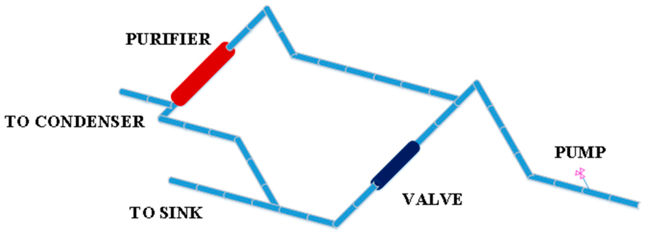
The experiment uses the approach of system identification to build the vibration transfer function across points between the brake and the sensor in the distributed piping system. The purpose of this treatment is to analyse the performance of the system more effectively and visualize the control effect of the controller. The input and output experimental data calculated by the finite element model are identified with the aid of the system identification toolbox by choosing the appropriate number of zeros and poles, and the parameters of the transfer function are optimized using the particle swarm optimization algorithm to bring the output value of the transfer function model closer to the output value calculated by the finite element mode. The sampling time of the system is 0.001 s, and a total of 10,000 moments are taken, that is, data within 10 s.

The cross-point vibration transfer function between the system brake and the sensor identified by the system identification toolbox is

$$G\left(z\right)=\frac{0.0013z^{-1}}{1+0.6362z^{-1}+0.4028z^{-2}}$$

(3)

A random search swarm intelligence optimization algorithm called particle swarm optimization (PSO) mimics the foraging behaviour of birds. It is frequently utilized in a variety of complex and nonlinear optimization problems because of its advantages of quick convergence speed and excellent convergence accuracy. The velocity and position update formulas of PSO are shown in Formulas (4) and (5):

$$\begin{gathered} v_i=v_i+c_{1}rand\times \left(pbes{t}_i-x_i\right) \\ +c_{2}rand\times \left(gbes{t}_i-x_i\right), \end{gathered}$$

(4)

$$x_i=x_i+v_i,i=1,2,\dots ,n$$

(5)

In the formula, v_i is the particle update speed, c₁ and c₂ are the algorithm learning factors, pbest_i is the individual optimal solution, gbest_i is the global optimal solution, x_i is the current particle position, and n is the number of particles in the population.

The PSO algorithm takes the model matching degree between the transfer function model and the finite element model as the optimization goal. The model matching the degree Formula is as follows:

$$J=1-\sqrt{\frac{{{\displaystyle \sum }}_{i=1}^M{\left(y_i\left(t\right)-{y^{\prime }}_i\left(t\right)\right)}^2}{{{\displaystyle \sum }}_{i=1}^M{\left(y_i\left(t\right)-\overline{y}\left(t\right)\right)}^2}}$$

(6)

In the formula, $y_i\left(t\right)$ is the finite element output at the ith sampling time, and ${y^{\prime }}_i\left(t\right)$ is the output of the transfer function model at the ith sampling time. If the degree of similarity between the identified model and the real model is higher, the model’s fit index J is closer to 1. The parameters of PSO are set as c₁ = 0.9, c₂ = 1.2. The cross-point vibration transfer function between the system brake and the sensor obtained after the optimization of PSO is

$$G\left(z\right)=\frac{3.2579\times {10}^{-4}+0.0015z^{-1}}{1+0.6361z^{-1}+0.4028z^{-2}}$$

(7)

Then, the transfer Function (7) is converted from a discrete model to a continuous model as follows:

$$G\left(s\right)=\frac{0.0003258s^2+2.548s+4011}{s^2+909.4s+4.599\times {10}^6}$$

(8)

Table 1. Comparison results of the transfer function and finite element model.

Method	Difference in Signal Energy	Model Fit
The system Identification toolbox	0.8042	83.09%
Particle swarm optimization	0.6148	88.03%

compares the outcomes of transfer function optimization using the PSO approach and the system identification toolbox. The table analysis demonstrates that the transfer function optimized by PSO is closer to the vibration signal energy of the finite element model with a higher degree of matching, which can be further increased after identification by the system identification toolbox. The design environment of the subsequent controller is more closely aligned with the distributed piping system due to the model’s correctness.

4. Design of the Fractional-Order PID Controller

Since the introduction of the order increases the complexity of controller parameter optimization, this section adopts a D-decomposition algorithm to select the parameters of the FOPID controller. Considering the cross-point vibration transfer function between the system brake and the sensor as a second-order system, Equation (9) gives the expression of the plant based on the model in the paper [28]:

$$G\left(s\right)=\frac{n_2{s}^{q_2}+n_1{s}^{q_1}+n_0{s}^{q_0}}{m_2{s}^{p_2}+m_1{s}^{p_1}+m_0{s}^{p_0}}\triangleq \frac{N\left(s\right)}{D\left(s\right)},$$

(9)

Among these, p and q are the orders of D(s) and N(s), respectively, and satisfy the inequalities p₂ > p₁ > p₀ and q₂ > q₁ > q₀. M and n are the coefficients of D(s) and N(s), respectively. When the p and q values are integers, the system is an integer-order system. When the p and q values are fractional, the system is a fractional-order system.

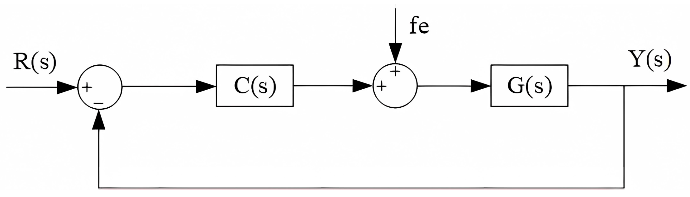
Figure 2 shows the system structure of the controlled object under the fractional-order PID controller.

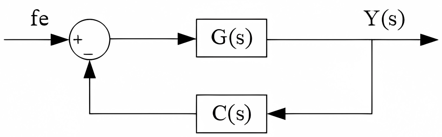
In the diagram, R(s) stands for the system’s input, Y(s) is the output, and f_e is the external effect which mostly refers to the piping system’s excitation force. The controller and control object, respectively, are denoted by C(s) and G(s). In the vibration reduction control problem of the distributed piping system, to reduce the output value of vibration as much as possible, the input value (expected value) R(s) is set to zero, that is, R(s) = 0, the system structure diagram can be equivalent to Figure 3.

According to Formula (2), the fractional-order PID controller can be expressed as $C\left(s\right)=k_p+\frac{k_i}{s^{\lambda }}+k_d{s}^{\mu }$. Therefore, the open-loop transfer function of the system can be determined from the figure as follows:

$$P_o\left(s\right)=C\left(s\right)G\left(s\right)=\frac{\left(k_p{s}^{\lambda }+k_i+k_d{s}^{\lambda +\mu }\right)N\left(s\right)}{s^{\lambda }D\left(s\right)}$$

(10)

The closed-loop transfer function of the system is

$$P_c\left(s\right)=\frac{G\left(s\right)}{1+C\left(s\right)G\left(s\right)}=\frac{s^{\lambda }N\left(s\right)}{s^{\lambda }D\left(s\right)+\left(k_p{s}^{\lambda }+k_i+k_d{s}^{\lambda +\mu }\right)N\left(s\right)}$$

(11)

Then, an operator of system (11) is defined as

$$L\left(s\right)=s^{\lambda }D\left(s\right)+\left(k_p{s}^{\lambda }+k_i+k_d{s}^{\lambda +\mu }\right)N\left(s\right)$$

(12)

It is possible to derive the operator L(s) expression with respect to the controller parameters k_p, k_i, k_d, λ and μ.

$$L\left(s,k_p,k_i,k_d,\lambda ,\mu \right)={{\displaystyle \sum }}_{\sigma =0}^2{m}_{\sigma }{s}^{p_0+\lambda }+n_{\sigma }{s}^{q_{\sigma }}(k_p{s}^{\lambda }+k_i+k_d{s}^{\lambda +\mu }),$$

(13)

The values of the controller parameters k_p, k_i, k_d, λ and μ determine the position and area of the stability region (SR) of the system. Real root boundaries (RRB), infinite root boundaries (IRB), and complicated root boundaries (CRB) make up the majority of the boundaries of SR. The three boundaries are described in the D-decomposition approach as follows:

RRB: When s = 0, the parameter condition when the operator L = 0 is made,

$$L\left(s=0,k_p,k_i,k_d,\lambda ,\mu \right)=n_0{s}^{q_0}{k}_i=0$$

(14)

IRB: In the literature [28], the author shows that the condition for the existence of IRB is p_n ≤ q_n + μ, and p_n and q_n are the highest orders of polynomial D(s) and N(s), respectively. On this basis, IRB can be expressed as

$$k_d=\{\begin{array}{c}0 if\left(p_n=q_n\right)or(p_n>q_n,\mu >p_n-q_n)\\ \pm \frac{m_2}{n_2} if(p_n>q_n,\mu =p_n-q_n) \\ none if\left(p_n>q_n,\mu <p_n-q_n\right) \end{array}$$

(15)

To ensure the existence of the differential part in the controller, that is, the coefficient k_d ≠ 0, the differential order μ needs to satisfy the condition μ ≤ p_n − q_n.

CRB: Bring s = jω into Formula (13) and make its value equal to 0, then CRB can be defined as

$$L\left(j\omega ,k_p,k_i,k_d,\lambda ,\mu \right)={\displaystyle \sum }_{\sigma =0}^2{m}_{\sigma }{\left(j\omega \right)}^{p_0+\lambda }+n_{\sigma }j{\left(\omega \right)}^{q_{\sigma }}\left(k_p{s}^{\lambda }+k_i+k_d{\left(j\omega \right)}^{\lambda +\mu }\right)=0$$

(16)

The expressions for the controller parameters k_p, k_i, k_d, λ, μ and ω can be derived from Formula (16):

$$\begin{gathered} {\Gamma }_1{H}_1\left(\omega ,\lambda \right)+k_p{H}_2\left(\omega ,\lambda \right)+k_i{H}_3\left(\omega \right)+k_d{H}_4\left(\omega ,\lambda ,\mu \right)=0 \\ \left(\omega ,\lambda \right)+k_p{\Gamma }_2\left(\omega ,\lambda \right)+k_i{\Gamma }_3\left(\omega \right)+k_d{\Gamma }_4\left(\omega ,\lambda ,\mu \right)=0, \end{gathered}$$

(17)

where

$$\begin{gathered} {\Gamma }_1\left(\omega ,\lambda \right)={{\displaystyle \sum }}_{\sigma =0}^2{m}_{\sigma }{\omega }^{p_{\sigma }+\lambda }\cos \frac{\left(p_{\sigma }+\lambda \right)\pi }{2} \\ {\Gamma }_2\left(\omega ,\lambda \right)={{\displaystyle \sum }}_{\sigma =0}^2{n}_{\sigma }{\omega }^{q_{\sigma }+\lambda }\cos \frac{\left(q_{\sigma }+\lambda \right)\pi }{2} \\ {\Gamma }_3\left(\omega \right)={{\displaystyle \sum }}_{\sigma =0}^2{n}_{\sigma }{\omega }^{q_{\sigma }}\cos \frac{q_{\sigma }\pi }{2} \\ {\Gamma }_2\left(\omega ,\lambda \right)={{\displaystyle \sum }}_{\sigma =0}^2{n}_{\sigma }{\omega }^{q_{\sigma }+\lambda +\mu }\cos \frac{\left(q_{\sigma }+\lambda +\mu \right)\pi }{2} \\ {H}_1\left(\omega ,\lambda \right)={{\displaystyle \sum }}_{\sigma =0}^2{m}_{\sigma }{\omega }^{p_{\sigma }+\lambda }\sin \frac{\left(p_{\sigma }+\lambda \right)\pi }{2} \\ {H}_2\left(\omega ,\lambda \right)={{\displaystyle \sum }}_{\sigma =0}^2{n}_{\sigma }{\omega }^{q_{\sigma }+\lambda }\sin \frac{\left(q_{\sigma }+\lambda \right)\pi }{2} \\ {H}_3\left(\omega \right)={\displaystyle \sum }_{\sigma =0}^2{n}_{\sigma }{\omega }^{q_{\sigma }}\sin \frac{q_{\sigma }\pi }{2} \\ {H}_4\left(\omega ,\lambda ,\mu \right)={\displaystyle \sum }_{\sigma =0}^2{n}_{\sigma }{\omega }^{q_{\sigma }+\lambda +\mu }\sin \frac{\left(q_{\sigma }+\lambda +\mu \right)\pi }{2} \end{gathered}$$

(18)

Through derivation, the expressions of the controller parameters k_p and k_i can be obtained as

$$k_p\left(\omega ,k_d,\lambda ,\mu \right)=\frac{{\Gamma }_3\left(\omega \right)H_1\left(\omega ,\lambda \right)-{\Gamma }_1\left(\omega ,\lambda \right)H_3\left(\omega \right)+k_d\left[{\Gamma }_3\left(\omega \right)H_4\left(\omega ,\lambda ,\mu \right)-{\Gamma }_4\left(\omega ,\lambda ,\mu \right)H_3\left(\omega \right)\right]}{{\Gamma }_2\left(\omega ,\lambda \right)H_3\left(\omega \right)-{\Gamma }_3\left(\omega \right)H_2\left(\omega ,\lambda \right)},$$

(19)

$$k_i\left(\omega ,k_d,\lambda ,\mu \right)=\frac{{\Gamma }_1\left(\omega ,\lambda \right)H_2\left(\omega ,\lambda \right)-{\Gamma }_2\left(\omega ,\lambda \right)H_1\left(\omega ,\lambda \right)+k_d\left[{\Gamma }_4\left(\omega ,\lambda ,\mu \right)H_2\left(\omega ,\lambda \right)-{\Gamma }_2\left(\omega ,\lambda \right)H_4\left(\omega ,\lambda ,\mu \right)\right]}{{\Gamma }_2\left(\omega ,\lambda \right)H_3\left(\omega \right)-{\Gamma }_3\left(\omega \right)H_2\left(\omega ,\lambda \right)}$$

(20)

4.1. Design of Parameters k_p, k_i, k_d

When the controller order parameters λ and μ are given, the value range of k_d can be obtained through SR as $0\to k_{dsup}$. According to the definition of the phase angle margin P_m and the crossover frequency ω_c,

$$\{\begin{array}{c}|P_o\left(s\right){|}_{s=j{\omega }_c}=1\\ \arg \left(P_o\left(s\right){|}_{s=j{\omega }_c}\right)=-\pi +P_m\end{array}$$

(21)

When bringing Formula (11) into Formula (21),

$$s^{\lambda }D\left(s\right)+\left(k_p{s}^{\lambda }+k_i+k_d{s}^{\lambda +\mu }\right)N\left(s\right){|}_{s=j{\omega }_c}=0$$

(22)

The relationship between the controller parameters k_p, k_i on k_d, λ, μ is then derived:

$$k_p\left(k_d,\lambda ,\mu \right)=\frac{{\Gamma }_{3c}{H}_{1c}\left(\lambda \right)-{\Gamma }_{1c}\left(\lambda \right)H_{3c}+k_d\left[{\Gamma }_{3c}{H}_{4c}\left(\lambda ,\mu \right)-{\Gamma }_{4c}\left(\lambda ,\mu \right)H_{3c}\right]}{{\Gamma }_{2c}\left(\lambda \right)H_{3c}-{\Gamma }_3{H}_2\left(\lambda \right)}$$

(23)

$$\begin{array}{l}{k}_i\left(k_d,\lambda ,\mu \right)\\ =\frac{{\Gamma }_{1c}\left(\lambda \right)H_{2c}\left(\lambda \right)-{\Gamma }_{2c}\left(\lambda \right)H_{1c}\left(\lambda \right)+k_d\left[{\Gamma }_{4c}\left(\lambda ,\mu \right)H_{2c}\left(\lambda \right)-{\Gamma }_{2c}\left(\lambda \right)H_{4c}\left(\lambda ,\mu \right)\right]}{{\Gamma }_{2c}\left(\lambda \right)H_{3c}-{\Gamma }_{3c}{H}_{2c}\left(\lambda \right)}\end{array}$$

(24)

where

$$\begin{gathered} {\Gamma }_{1c}\left(\lambda \right)={{\displaystyle \sum }}_{\sigma =0}^2{m}_{\sigma }{{\omega }_c}^{p_{\sigma }+\lambda }\cos \frac{\left(p_{\sigma }+\lambda \right)\pi }{2} \\ {\Gamma }_{2c}\left(\lambda \right)={{\displaystyle \sum }}_{\sigma =0}^2{n}_{\sigma }{{\omega }_c}^{q_{\sigma }+\lambda }\cos (\frac{\left(q_{\sigma }+\lambda \right)\pi }{2}-P_m) \\ {\Gamma }_{3c}={{\displaystyle \sum }}_{\sigma =0}^2{n}_{\sigma }{{\omega }_c}^{q_{\sigma }}\cos (\frac{q_{\sigma }\pi }{2}-P_m) \\ {\Gamma }_{4c}\left(\lambda ,\mu \right)={{\displaystyle \sum }}_{\sigma =0}^2{n}_{\sigma }{{\omega }_c}^{q_{\sigma }+\lambda +\mu }\cos (\frac{\left(q_{\sigma }+\lambda +\mu \right)\pi }{2}-P_m) \\ {H}_{1c}\left(\lambda \right)={{\displaystyle \sum }}_{\sigma =0}^2{m}_{\sigma }{{\omega }_c}^{p_{\sigma }+\lambda }\sin \frac{(p_{\sigma }+\lambda )\pi }{2} \\ {H}_{2c}\left(\lambda \right)={{\displaystyle \sum }}_{\sigma =0}^2{n}_{\sigma }{{\omega }_c}^{q_{\sigma }+\lambda }\sin (\frac{\left(q_{\sigma }+\lambda \right)\pi }{2}-P_m) \\ {H}_{3c}={{\displaystyle \sum }}_{\sigma =0}^2{n}_{\sigma }{{\omega }_c}^{q_{\sigma }}\sin (\frac{q_{\sigma }\pi }{2}-P_m) \\ {H}_{4c}\left(\lambda ,\mu \right)={{\displaystyle \sum }}_{\sigma =0}^2{n}_{\sigma }{{\omega }_c}^{q_{\sigma }+\lambda +\mu }\sin (\frac{\left(q_{\sigma }+\lambda +\mu \right)\pi }{2}-P_m), \end{gathered}$$

(25)

The following formula can be used to determine the controller parameter k_d to ensure that the system has the better performance:

$$P_o\left(j\omega \right)=\frac{Q\left(\omega ,k_d\right)+jR\left(\omega ,k_d\right)}{{\Gamma }_1\left(\omega ,\lambda \right)+j{H}_1\left(\omega ,\lambda \right)},$$

(26)

where

$$\begin{gathered} Q\left(\omega ,k_d\right)=k_p\left(k_d\right){\Gamma }_2\left(\omega ,\lambda \right)+k_i\left(k_d\right){\Gamma }_3\left(\omega \right)+k_d{\Gamma }_4\left(\omega ,\lambda ,\mu \right) \\ R\left(\omega ,k_d\right)=k_p\left(k_d\right)H_2\left(\omega ,\lambda \right)+k_i\left(k_d\right)H_3\left(\omega \right)+k_d{H}_4\left(\omega ,\lambda ,\mu \right) \end{gathered}$$

(27)

The argument of $P_o\left(j\omega \right)$ can be expressed as

$$\arg \left(P_o\left(j\omega \right)\right)=\arctan \Psi \left(\omega ,k_d\right)+n\pi$$

(28)

where n is an integer and

$$\Psi \left(\omega ,k_d\right)=\frac{R\left(\omega ,k_d\right){\Gamma }_1\left(\omega ,\lambda \right)-Q\left(\omega ,k_d\right){\Gamma }_1\left(\omega ,\lambda \right)}{Q\left(\omega ,k_d\right){\Gamma }_1\left(\omega ,\lambda \right)+R\left(\omega ,k_d\right)H_1\left(\omega ,\lambda \right)}$$

(29)

To achieve optimal robustness, the controller parameter k_d can be calculated using the following formula:

$$k_d=\underset{0\le k_d<k_{d\sup }}{\mathrm{argmin}}\left|{\frac{darg\left(P_o\left(j\omega \right)\right)}{d\omega }|}_{\omega ={\omega }_c}\right|$$

(30)

When the value of k_d is obtained by calculation, the values of the controller parameters k_p and k_i can be obtained according to Formula (12):

$$k_p=k_p\left(k_d\right),k_i=k_i\left(k_d\right)$$

(31)

The value range of parameter ω is $\left[{\omega }_{\min },{\omega }_{\max }\right]$, and the values of ${\omega }_{\min }$ and ${\omega }_{\max }$ satisfy the following conditions:

$$\begin{gathered} {\omega }_{\min }:k_p\left({\omega }_{\min }\right)=0 \mathrm{and} k_p\left({\omega }_{\min }^{+}\right)<0 \\ {\omega }_{\max }:{\omega }_{\max }>{\omega }_{\min },k_p\left({\omega }_{\max }\right)\ge 0 \end{gathered}$$

(32)

4.2. Design of Parameters λ and μ

The values of k_p, k_i and k_d only depend on the order λ and μ according to Formulas (30) and (31). The time multiplied by the integral of the absolute value of the error (ITAE) is chosen as the performance index of the controller to achieve the best response performance of the control system, i.e.,

$$J_{ITAE}={{\displaystyle \int }}_0^{\infty }t\left|e\left(t\right)\right|dt$$

(33)

Among them, e(t) is the error signal in the control system. By finding the λ and μ values that minimize the performance index J_ITAE value, the values of parameters k_p, k_i and k_d are further determined according to Formulas (30) and (31):

$$k_d=\underset{0\le k_d<k_{d\sup }}{\mathrm{argmin}}\left|{\frac{d(\arctan (\frac{R\left(\omega ,k_d\right){\Gamma }_1\left(\omega ,\lambda \right)-Q\left(\omega ,k_d\right)H_1\left(\omega ,\lambda \right)}{Q\left(\omega ,k_d\right){\Gamma }_1\left(\omega ,\lambda \right)+R\left(\omega ,k_d\right)H_1\left(\omega ,\lambda \right)})+n\pi )}{d\omega }|}_{\omega ={\omega }_c}\right|$$

(34)

$$k_p=k_p\left(k_d\right),k_i=k_i\left(k_d\right)$$

(35)

4.3. Design Process

In this section, the specific steps to obtain the parameters of the fractional-order controller using the D-decomposition method are given as follows.

Step 1 Initialize the following data, including

$$p_2,p_1,p_0,q_2,q_1,q_0,m_2,m_1,m_0,n_2,n_1,n_0.$$

Set the phase angle margin Pm and the crossover frequency ω_c.

Step 2 In order to ensure the existence of the differential part in the fractional order controller, according to Formula (15), it obtains k_d ≠ 0 and the differential order must satisfy the condition μ ≤ p_n − q_n. When the order parameters λ and μ gradually increase from low to high, the value range $0\to k_{dsup}$ of the controller parameter k_d is calculated according to SR.

Step 3 The values of the controller parameters k_p, k_i and k_d under the conditions of traversal $\lambda \in \left(0,2\right)$ and $\mu \in \left(0,2\right)$ are calculated sequentially through Formulas (34) and (35), and the performance index J_ITAE of the controller is calculated according to Formula (33).

Step 4 The planned fractional-order PID controller’s parameter value is determined by finding the values of k_p, k_i, k_d, λ and μ, that minimize the performance index J_ITAE.

5. Experimental Results

According to Formula (8), the controlled object of the system is

$$G\left(s\right)=\frac{0.0003258s^2+2.548s+4011}{s^2+909.4s+4.599\times {10}^6}$$

(36)

As can be seen from Formula (36), the coefficient of s² is much lower than the other coefficients, so it is simplified here. The transfer function G(s) can be approximated as

$$G^{\prime }\left(s\right)=\frac{2.548s+4011}{s^2+909.4s+4.599\times {10}^6}$$

(37)

The transfer functions $G^{\prime }\left(s\right)$ serve as the foundation for the fractional-order PID controller, and their initialisation $G^{\prime }\left(s\right)$ yields the following information:

$$G^{\prime }\left(s\right):\begin{array}{c}{p}_2=2,p_1=1,p_0=0, q_1=1, q_0=0,\\ m_2=1,m_1=909.4,m_0=4.599\times {10}^6,\\ n_1=2.548,n_0=4011.\end{array}$$

Set the phase angle margin P_m = 7π/10 and the crossover frequency ω_c = 1500, and calculate the RRB, IRB.

RRB: k_i = 0, IRB: k_d = none.

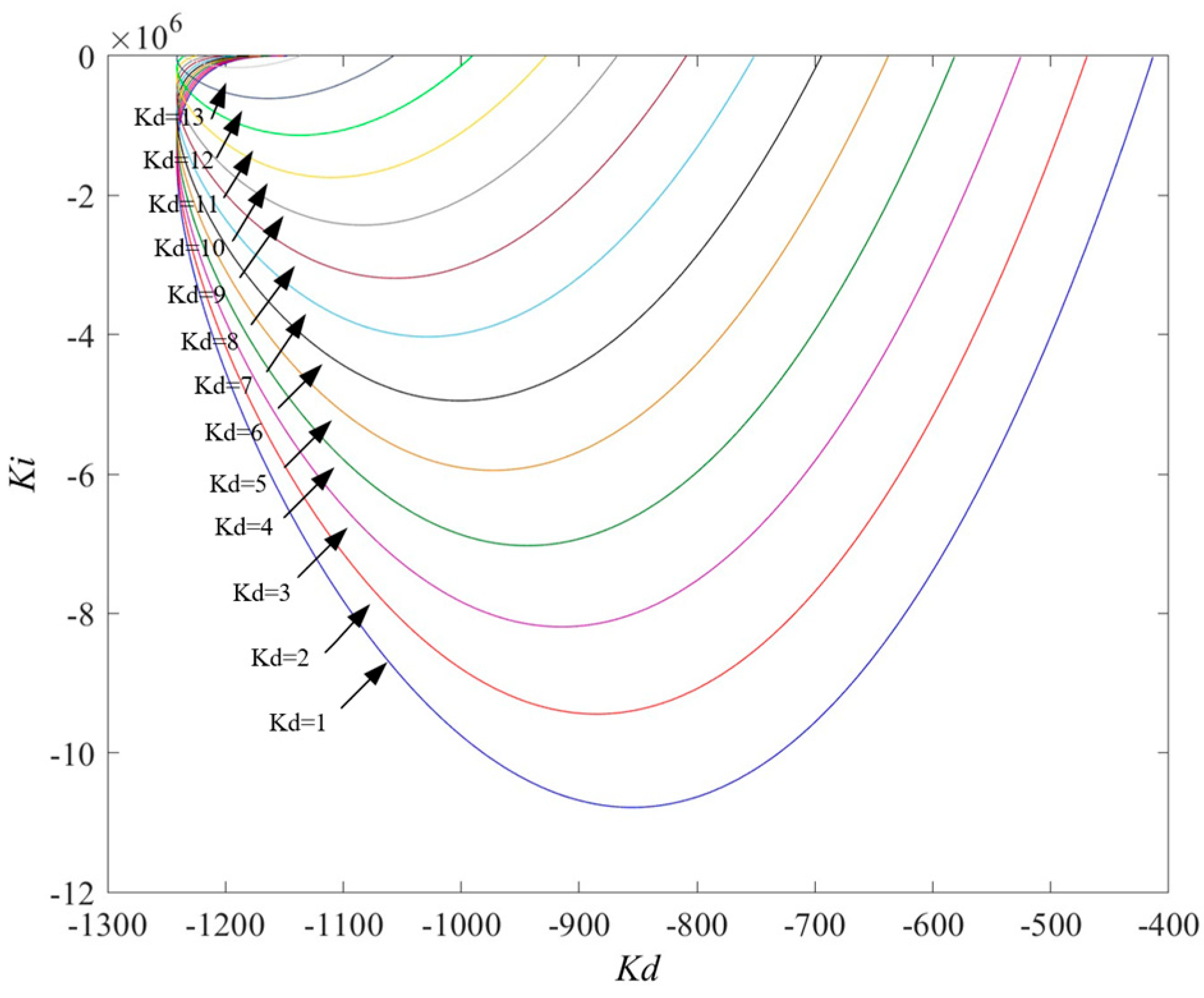
From Step 2, the value range of the order parameter of the fractional-order PID controller must be $\lambda \in \left(0,2\right)$ and $\mu \in \left(0,2\right)$. Calculate the position of the system stability interval SR under the conditions of different integral and differential orders and determine the value range of ω as [ω_min , ω_max]. Taking λ = 1.5 and μ = 0.5 as examples, the k_dsup value of the transfer functions is obtained as k_dsup = 13. Figure 4 shows the SR of the transfer functions $G^{\prime }\left(s\right)$ under different k_d values. From the graph analysis, as k_d increases, the SR area of the system gradually decreases.

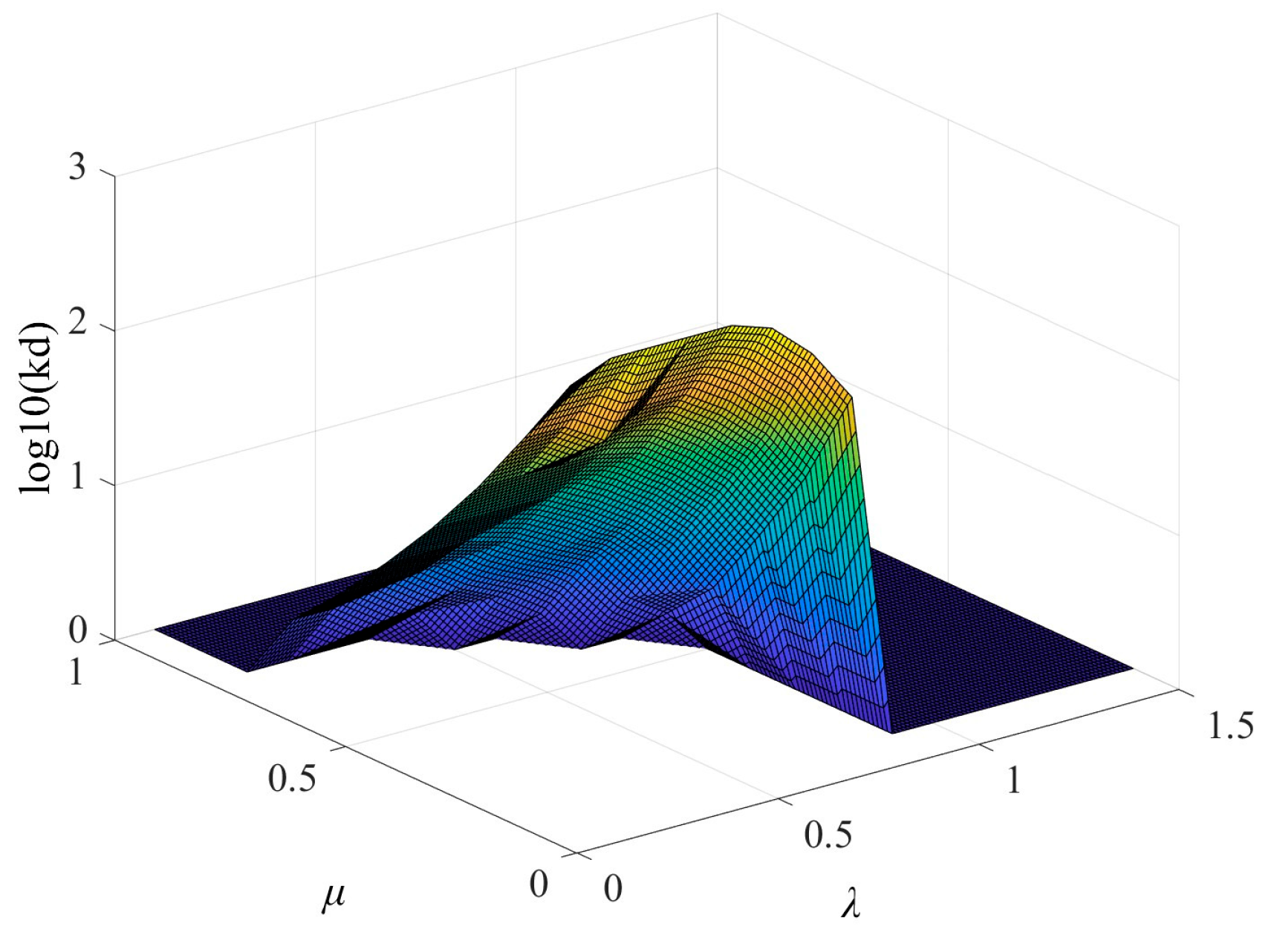
According to Formula (34), the relationship between the optimal k_d value and λ, μ under the conditions of different order parameters λ and μ is obtained, as shown in Figure 5.

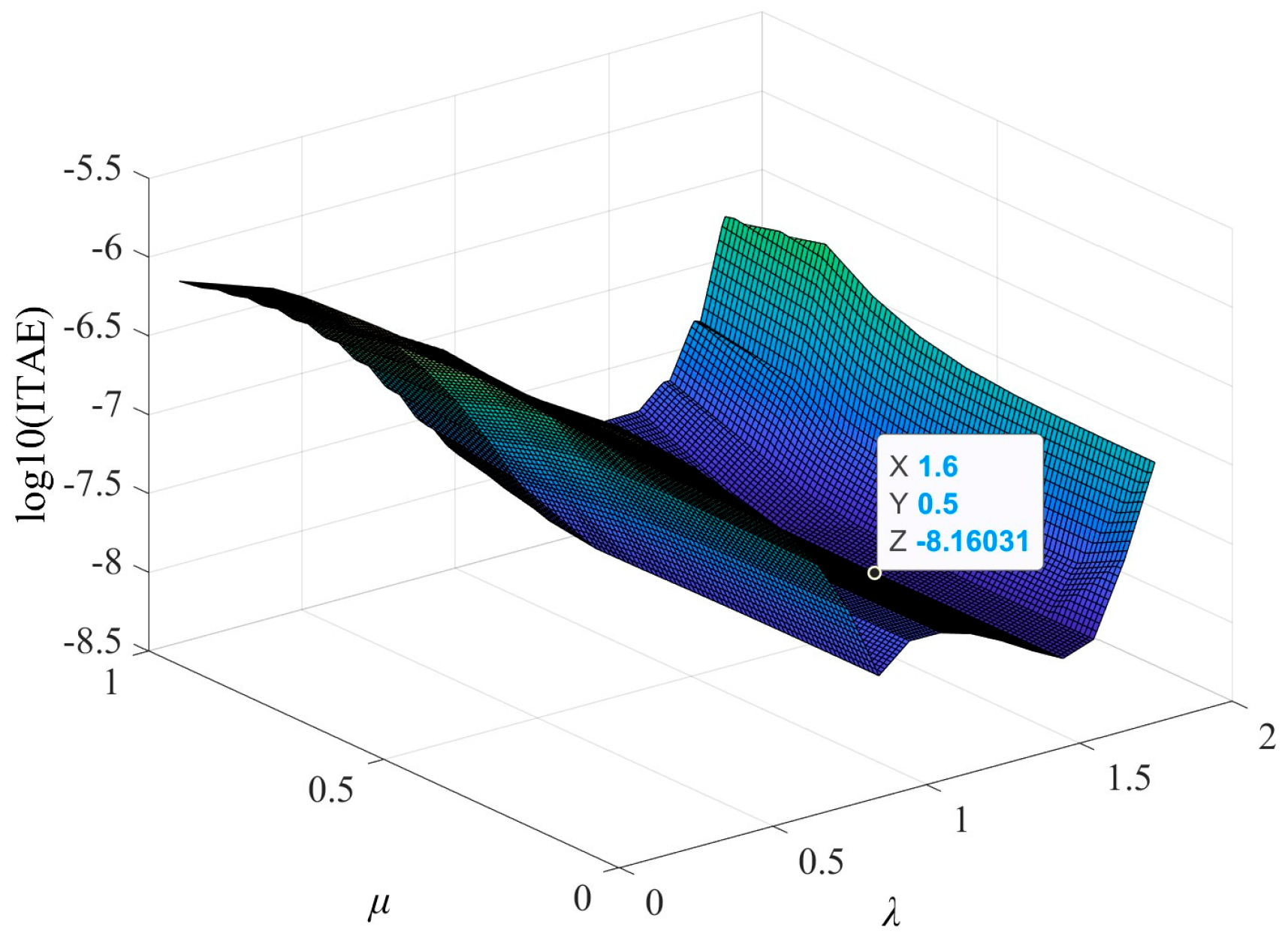
Given the parameters k_dbest, λ and μ, the performance index J_ITAE of the control system under different conditions is calculated. Figure 6 depicts the link between J_ITAE and parameters λ, μ. The graph analysis reveals that the integral order λ has a significant impact on the J_ITAE of the system while the differential order μ has less of an impact.

Under the condition of P_m = 7π/10 and ω_c = 1500, when the order parameters of the transfer function are λ = 1.6 and μ = 0.5, the minimum value of the performance index J_ITAE is J_ITAE = 6.913 × 10⁻⁹.

Consequently, the intended fractional-order PID controller parameters can be obtained as

$$C_1\left(s\right)=8.215 \times {10}^2+\frac{9.863 \times {10}^7}{s^{1.6}}+s^{0.5}$$

(38)

By setting the order to one and using the same method, the parameters of the PID controller are designed as follows:

$$C_2\left(s\right)=187.833+\frac{9.043 \times {10}^5}{\mathrm{s}}+0.100 \mathrm{s}$$

(39)

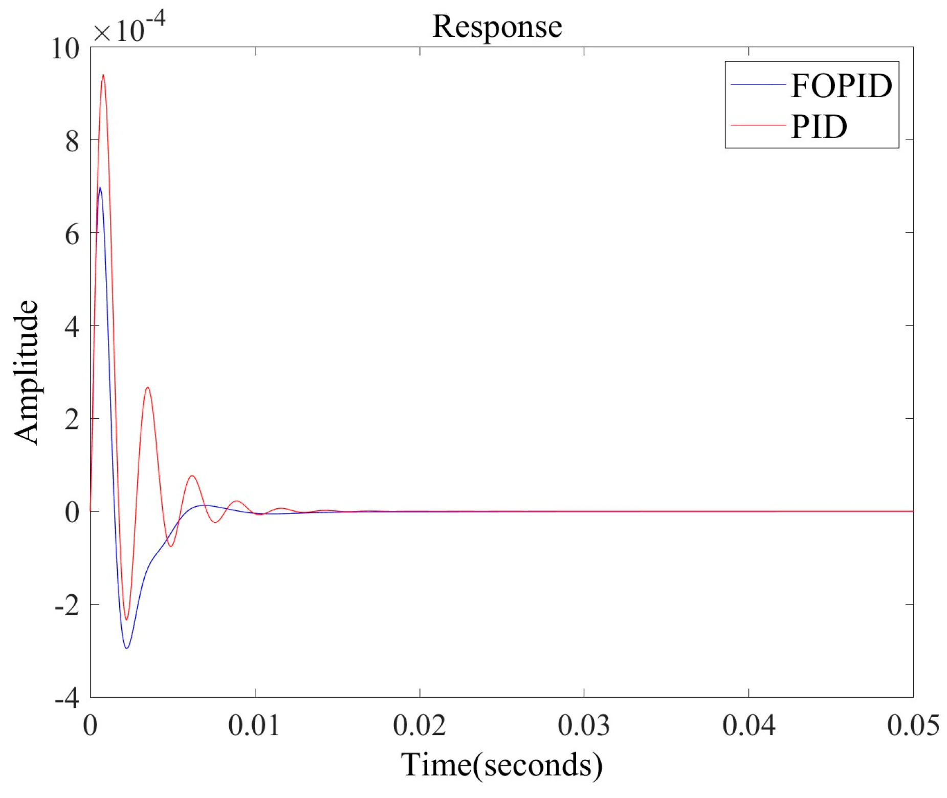
Figure 7 shows the responses of the transfer functions $G^{\prime }\left(s\right)$ under fractional-order and integer-order PID controls, indicating that the control system has a significant overshoot and many oscillations following the addition of the integer-order PID controller. Excessive overshoot significantly affects the system’s performance. In some practical engineering systems, an excessive overshoot may lead to devastating consequences that are not allowed. More oscillations and longer adjustment times also significantly reduced the system’s stability. The addition of the fractional-order PID controller reduces the system’s overshoot and the number of oscillations based on the PID controller, shortens the system’s adjustment time, significantly enhances the system’s performance, and boosts the quality and efficiency of control owing to the introduction of two parameters of the fractional-order PID controller, which makes the controller province more compatible with the controlled object and improves the controlled freedom.

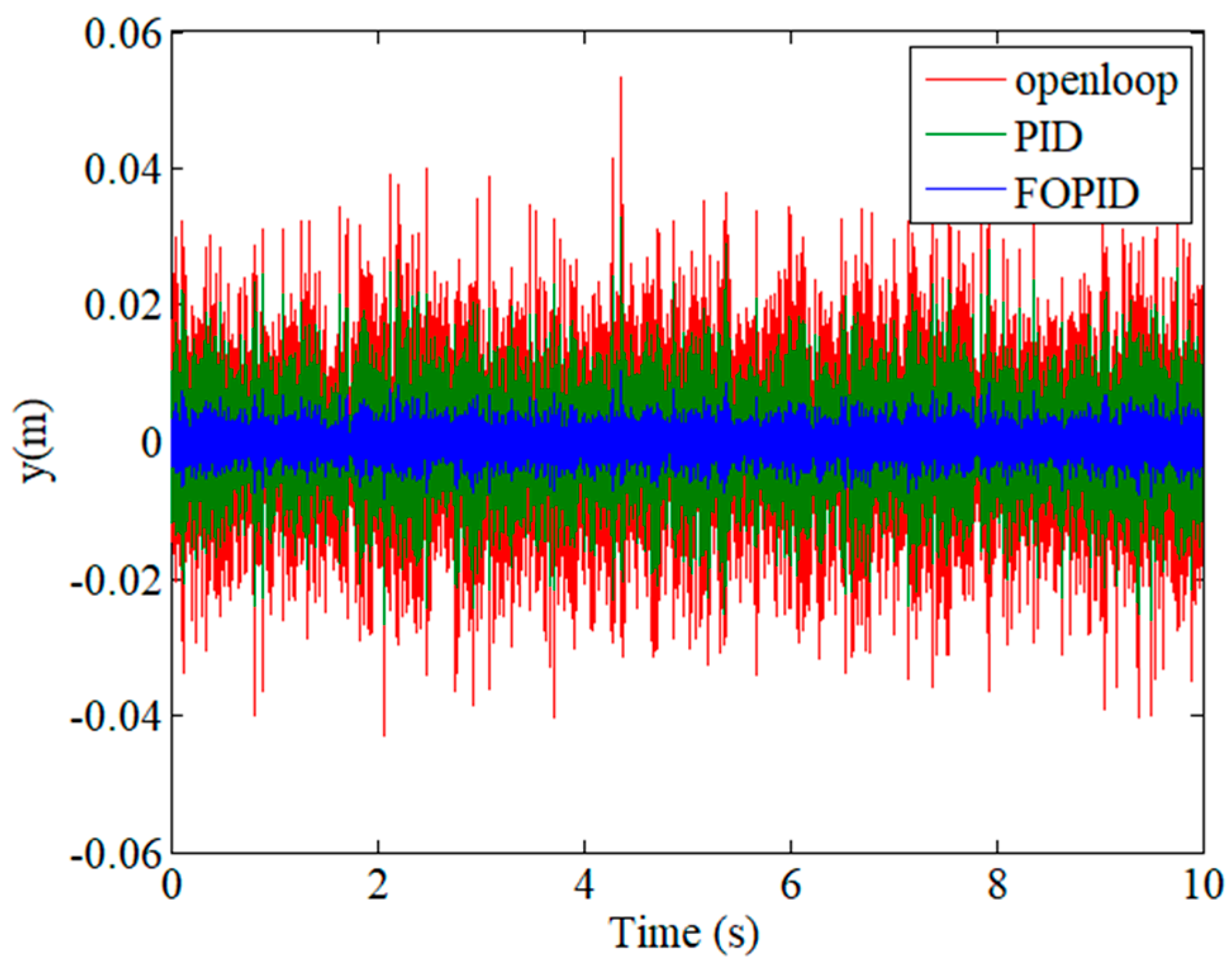
Figure 8 shows the output of the system vibration for a distributed piping system without a controller, with a PID controller and with a fractional-order PID controller. The PID controller can reduce the vibration of the piping system. According to the analysis shown in the figure, its control effect is limited. However, this approach is insufficient for demanding control systems. The fractional-order PID controller, based on the PID controller, can further reduce the vibration output of the piping system. The vibration amplitude can be maintained within a particular range, thereby reducing damage to the pipeline and improving its continuous use time. Therefore, the reference of the integral order λ and differential order μ in a fractional-order PID controller can improve the control precision of the controller and obtain a better control effect.

6. Conclusions

This study proposes a design approach for a fractional-order proportional–integral–derivative (PID) controller for vibration reduction in distributed piping systems. This technique uses the D-decomposition approach to determine the IRB, CRB, and RRB boundaries of the SR and achieves the best possible control of the controlled object by lowering the system’s JITAE performance index. In the process of system identification of the pipe network, the system identification toolbox was used to realise the system identification of the vibration transfer function between the brakes and the sensor. A comparative analysis showed that the transfer function has the potential to further improve the degree of fit of the model. Therefore, PSO was adopted, and the matching degree of the transfer function model was used as the optimisation goal. The parameter values of the transfer function were further optimised such that the calculated and improved transfer function was closer to the finite element model in terms of accuracy. Subsequently, a fractional-order PID controller designed using the D-decomposition method was applied to the transfer function. The experimental results demonstrate that the proposed fractional-order PID controller can significantly minimise the overshoot of the original system, number of oscillations, and adjustment time. In addition, it has a substantially better suppressive effect on pipeline vibrations than the PID controller. Consequently, a fractional-order PID controller is more suitable for suppressing vibrations in the distributed piping system of a power plant. Considering their superiority over integer-order PID controllers, fractional-order PID controllers in different fields remain an exploratory direction for future work.