Finite Difference Modeling of Time Fractal Impact on Unsteady Magneto-hydrodynamic Darcy–Forchheimer Flow in Non-Newtonian Nanofluids with the q-Derivative

Abstract

This contribution addresses a fractal numerical scheme that can be employed for handling fractal time-dependent parabolic equations. The numerical scheme presented in this contribution can be used to discretize integer order and fractal derivatives in a given differential equation. Therefore, the scheme and results can be used for both cases. The proposed finite difference scheme is based on two stages. Fractal time derivatives are discretized by employing the proposed approach. For the scalar convection–diffusion equation, we derive the stability condition of the proposed fractal scheme. Using a nonlinear chemical reaction, the approach is also used to solve the Quantum Calculus model of a Williamson nanofluid’s unsteady Darcy–Forchheimer flow over flat and oscillatory sheets. The findings indicate a negative correlation between the velocity profile and the porosity parameter and inertia coefficient, with an increase in these factors resulting in a drop in the velocity profile. Additionally, the fractal scheme under consideration is being compared to the fractal Crank–Nicolson method, revealing that the proposed scheme exhibits a superior convergence speed compared to the fractal Crank–Nicolson method. Several problems involving the motion of non-Newtonian nanofluids through magnetic fields and porous media can be investigated with the help of the proposed numerical scheme. This research has implications for developing more efficient heat transfer and energy conversion devices based on nanofluids.

1. Introduction

Since their major application in numerous industrial and engineering domains, the study of fluid dynamics, magnetohydrodynamics (MHDs), and nanofluids has experienced a spectacular boom in recent years. Theoretical studies of such intricate fluid flows are now crucial to improving the efficiency of cutting-edge tools, power grids, and ecological systems.

The unsteady magneto-hydrodynamic (MHD) Darcy–Forchheimer flow of nanofluids stands out as a crucial area of study among the wide variety of fluid flows. These nanofluids’ unusual thermal, electrical, and mechanical properties, when in a base fluid infused with nanoparticles, make them more relevant in heat transfer enhancement, electronic cooling, and biological applications.

Researchers have also recently begun investigating how q-derivatives might be used to model intricate physical events. The fractional calculus theory provides a new angle for characterizing the erratic and non-differentiable behaviors seen in time fractal events through the concept of $q$-derivatives. When applied to the finite difference method, q-derivatives provide more precise answers to difficult time-dependent situations.

Sub-categories of fluids have been developed over time based on their qualities. In early 1995, Choi [1] introduced a new category of fluids termed nanofluids. These fluids consist of metallic nanoparticles suspended in a base fluid. The metallic components enhance the thermo-physical characteristics of the fluid under investigation. Nevertheless, due to the minuscule size of the particles, it is possible to regard the complete saturation as a fluid, referred to as a nanofluid, which satisfies the requirements for non-Newtonian fluids. Since then, many research publications have covered a wide range of properties from various perspectives in industry, engineering, physics, and mathematics. In a study conducted by [2], it was observed that an incompressible radiative flow of nanofluids consistently traverses the surface of Riga. In this model, fluid movement, heat transfer, and mass transport are all assisted by the Lorentz forces produced by the Riga plate. Bai et al. [3] examined nanofluids’ MHD stagnation point flow, including the variations in heat and mass transport. The model was improved by adding new parameters, most notably one that affects heat flow directly—the radiation parameter. To address the governing equations, the authors in reference [4] formulated a mathematical representation of the flow behavior of a Maxwell nanofluid over a convectively heated surface. They then utilized the bvp4c method to solve this formulated model. Dogonchi et al. [5] used computational fluid dynamics (CFDs) to discuss the MHD flow of a Cu-Water nanofluid in a cavity.

Many manufacturing and engineering setups utilizing nanofluids can benefit from the fluid flow a stretching surface induces. Nanofluids have gained recognition for their various applications, such as surface stretching in industrial processes like melt-spinning and glass fiber manufacture, as well as for cooling metallic plates and manufacturing rubber bands and plastic sheets, among other purposes. Hydromagnetic fluid flow through a solid surface was attempted by Skiadis [6]. In a later paper, Crane [7] described a two-dimensional MHD flow driven by a deforming/stretching surface. Many recent studies focus on issues associated with linear and nonlinear stretching rates.

Nanofluid flows over a nonlinearly expanding sheet/surface exhibit some interesting variations in heat and mass transfer, as observed by Rasool et al. [8]. In a separate scholarly publication, the authors [9] provided a comprehensive account of the characteristics associated with the Cattaneo–Christov theory about transferring heat and mass over a surface that undergoes nonlinear stretching. Additionally, the authors discussed the Darcy relation and the field of magnetohydrodynamics (MHDs). The findings were achieved by adopting a homotopy strategy. The study concluded with a correlation summarizing the findings about the correlation between heat and mass flux. The theoretical behavior of a dusty nanofluid through a stretched sheet was analyzed by Sandeep et al. [10]. The study conducted by [11] focused on investigating heat source/sink properties and tilting magnetohydrodynamics (MHDs) in the context of nanofluid flow driven by a linear stretching surface. The homotopy method was used for reporting the findings. The resulting thermal layer curves are quite interesting. The significance of a permeable surface in a nanofluid flow due to stretching was demonstrated by Ziaei-Red et al. [12]. The results jibed well with the antecedent research.

Pseudoplastics are in high demand because of the unique features they possess. Some of the various uses for these materials include photographic film melts, solutions of polymers with higher molecular weights, suspensions, the expulsion of sheets, etc. Several models for describing this type of fluid flow have been developed in the literature, but the complexity of rheological systems prevents them from being fully adequate. The literature reports several models discussing the properties of such pseudoplastic materials, including those developed by Carreau, Cross, Ellis, and the power law model. However, there are viable alternatives to the original Navier Stokes equations, such as the Powell–Eyring and Williamson models. For those above-mentioned complex pseudoplastic materials, Williamson [13] conducted experimental research complemented by a model that bears his name and is known as the Williamson model. Subsequently, many studies reporting results similar to Williamson’s have been reported. The characteristics of the momentum boundary layer in the flow of a fluid across a flat surface were addressed by Blasius [14]. Ramesh et al. [15] used convective boundary conditions to merge the ideas of Blasius [14] and Sakiadis [6] with Williamson fluid. Homotopy was used to obtain these findings. A fascinating article on Williamson nanofluid flows around a cone was presented by Khan et al. [16]. The plate was brought up as a specific situation as well. According to the results, the temperature profile flattens out for higher Prandtl values, but it flattens out more for greater thermophoretic forces. Williamson fluids over a nonlinear variable surface were the subject of an MHDs study by Hayat et al. [17]. Over a stretching surface, where the fluid in question is assumed to be a Williamson fluid, Nadeem et al. [18] described the mechanism by which fluid flows, heats, and transports mass. The Williamson fluid flow across a stretching surface was described by Salahuddin et al. [19], who applied Cattaneo–Christov’s theory of heat and mass transfer. At the same time, convective conditions were used by Hayat et al. [20] to report Soret and Dufour’s impacts on the Williamson fluid flow. The results show that thermal and solute Biot numbers positively affect the temperature field.

A numerical model for a nanofluid convective vehicle has been proposed by Boungiorno [21]. He discovered that Brownian motion and thermophoresis are the primary causes of the slide. Tiwari and Das [22] investigated improved the heat transfer of nanofluids in a two-sided, top-driven, warmed square depression. Within a nuclear reactor control vessel, magneto-hydrodynamic streams through the extended surface play a significant role in oil design, projection, metalwork, and surface cooling. Large-scale medical applications for MHDs include drug delivery, attractive cell detachment, blood loss reduction during surgeries, therapy for certain blood vessel infections, and hyperthermia. The MHD flow of a dusty liquid was investigated by Makinde and Chinyoka [23] between two isothermal surfaces. Jalilpour et al. [24] investigated a nanofluid’s non-symmetric stagnation point MHD stream in the context of warm radiation across an expanding sheet. The study by [25] investigated the impact of a modified attractive field on the movement of attractive nanofluids in conjunction with graphene nanoparticles within a thin layer. The study by [26] investigated the peristaltic transport of magneto-hydrodynamic nanofluids, focusing on the impacts of joule heating and duct flexibility. The Williamson liquid, characterized by its shear-thinning behavior, is a noteworthy illustration of a non-Newtonian liquid model. The study by [27] examined the two-dimensional evolution of Williamson liquid over a stretched surface. The researchers engaged in a discussion regarding the effects of nanoparticles on Williamson fluid. Additionally, reference [28] investigated the influence of material reactions on the boundary layer flow of magnetohydrodynamics (MHDs) and the convective heat transfer of Williamson nanofluid in porous media.

Forchheimer [29] dissected latency and bounds using a square speed concept in Darcian speed. The Forchheimer factor was mentioned by Muskat [30]. Regarding the magnetic flux in the Darcy–Forcheimer regime, Sadiq and Hayat [31] looked at the behavior of a Maxwell fluid under the confines of a convectively heated sheet. A micropolar nanofluid Darcy–Forchheimer flow with non-uniform heat age/retention was investigated by Khan et al. [32]. The plates followed a pivoting outline. When the cross-over speed and the porosity boundary are both increased, an impermeable gap acts as a barrier in the stream’s path and slows the water’s flow. Using techniques for a curved extended surface with Cattaneo–Christov twofold dispersion, The Darcy–Forchheimer stream was evaluated by [33]. The Darcy–Forchheimer stream was separated into two halves along a curved surface with significant elongation, utilizing Cattaneo–Christov’s twofold dispersion [34]. In their study, the researchers in [35] undertook a mathematical inquiry into the behavior of the Darcy–Forchheimer flow on a curved expanding surface, considering the influence of a Cattaneo–Christov thermal transition and homogeneous–heterogeneous processes. The capacity to travel through a porous substance is particularly useful in studying geophysical liquid components. The human lung, sandstone, sandy seashores, limestone, nerve bladder, and the bile and vein systems devoid of stones are normally permeable media. The subtleties of permeable media in their many forms are considered. Rasool et al. [36] used mathematics to study the MHD Darcy–Forchheimer Williamson nanofluid stream through a nonlinearly expanding surface, looking for impacts of age entropy and parallel compound responses. The Buongiorno model’s liquid flow, mass and heat transfer, and entropy components were all measured using the second law of thermodynamics.

This work uses q-derivatives for the spatial discretization to learn more about Williamson nanofluid’s time fractal unsteady MHD Darcy–Forchheimer flow. For a long time, it has been understood that finite difference schemes are effective numerical tools for solving the partial differential equations that underpin a wide range of fluid flow issues. Using q-derivatives allows us to simulate time fractal phenomena and complex fluid flows with non-trivial behaviors, as we can capture the non-local aspects of the fractional order derivatives. The study has the three following aims:

• To create a mathematical model of the Williamson nanofluid’s unsteady MHD Darcy–Forchheimer flow, considering the effects of the nanoparticles, magnetic field, and porous media.
• To properly reflect the complex dynamics of time fractal events by incorporating the idea of q-derivatives into the spatial discretization scheme.
• To better understand the complex behavior of time-dependent flow parameters, such as velocities, temperatures, and concentration profiles, in the presence of magnetic fields and porous media by developing and analyzing a finite difference scheme to generate numerical solutions.

The results of this investigation should help advance our theoretical understanding of complicated fluid dynamics and inform efforts to enhance the functionality of systems based on nanofluids. Further, including q-derivatives into the finite difference method can provide novel approaches to the difficult time fractal phenomena found in many scientific fields.

There exists literature that deals with the numerical schemes of differential equations with classical derivatives. From the class of time-discretizing schemes, both types of schemes have been proposed by numerous researchers for solving time-dependent partial differential equations. One class of finite difference schemes is the time-stepping schemes. These schemes require information at different time levels, and some accuracy can be obtained. On the other hand, multi-stage schemes only utilize two time levels, and these schemes can solve differential equations with different accuracies. Most of the contributions in the literature have dealt with classical derivatives, but in this work, a fractal scheme that can be used to handle fractal parabolic equations is proposed. These schemes can be useful for those partial differential equations containing first-order time derivatives. Heat and mass transfer in a Darcy–Forchheimer flow of a Williamson nanofluid over flat and oscillatory sheets are solved using this approach. It is shown that the scheme works well in practice and that, when compared to the fractal Crank–Nicolson scheme, the suggested system converges more quickly.

Because nanoparticle behavior and their interactions with the fluid depart from the assumptions of classical fluid dynamics, it is essential to grasp that the fractional derivative enables us to express these complexities. The fractional derivative considers anomalous diffusion and memory effects, which can impact nanoparticle movement and temperature distribution in a nanofluid. Although the introduction of the fractional derivative may not always have a concrete physical analog, it is widely acknowledged to be a useful method for investigating complex fluid dynamics systems, such as nanofluids. To more accurately reflect the non-local and non-symmetric phenomena observed in nanofluid transport, researchers have found that fractional calculus is useful. A mathematical adaptation is consistent with the complexity of the system under examination, not a departure from physical principles. It also recognizes the controversy surrounding the use of fractional calculus in fluid dynamics.

The decision to incorporate a fractal time derivative into our computational method is driven by the intention to investigate and comprehend the dynamics of time-dependent parabolic equations when subjected to non-integer-order derivatives. Using integer-order derivatives is a primary feature of Newton’s second law and classical physics. However, the exploration of fractional calculus has uncovered captivating phenomena and applications throughout diverse scientific fields.

In our specific investigation, the utilization of fractal time derivatives holds particular significance for addressing the dynamics of unsteady magneto-hydrodynamic (MHD) Darcy–Forchheimer flow in non-Newtonian nanofluids. Incorporating these derivatives allows the influence of fractality on the system’s dynamics to be examined, offering valuable insights that may not be attainable only through traditional derivatives.

Although we recognize the established foundation of Newtonian derivatives within classical physics, our research adds to the expanding body of literature investigating the suitability and benefits of fractional derivatives in elucidating certain physical phenomena. We anticipate that our research article will stimulate additional discourse and an exploration of the application of non-integer-order derivatives in fluid dynamics and its associated disciplines.

Definition 1

([37]). The fractal derivative of a function $u\left(t\right)$ with respect to a fractal measure $t$ is defined as

$$\frac{du\left(t\right)}{d{t}^{\alpha }}=\underset{t_1\to t}{\lim }\frac{u\left(t_1\right)-u\left(t\right)}{t_1^{\alpha }-t^{\alpha }}, \alpha >0$$

Definition 2

([38]). The $q$-derivative of a function $v\left(x\right)$ is defined as

$${\left(\frac{d}{dx}\right)}_{q}v\left(x\right)=\frac{v\left(qx\right)-v\left(x\right)}{qx-x}, 0<q<1$$

Within the realm of investigations about the $q$-derivative or fractional calculus, assigning the quantum parameter $q$ a value of $1$ carries distinct ramifications of both a physical and mathematical nature.

Mathematical Implication: When the value of $q$ is set to $1$, the $q$-derivative operator is indistinguishable from the conventional classical derivative. In alternative terms, it returns to the conventional calculus operator. This implies that all equations or expressions containing derivatives with respect to$q$, where $q$ is equal to $1$, should be simplified to their classical counterparts.

Physical Implication: $q$-derivatives are frequently employed in studying physical systems to characterize non-classical phenomena, such as anomalous diffusion or the flow of non-Newtonian fluids. When the value of $q$ is equal to $1$, the system characterized by the $q$-derivative returns to a state at which it behaves in a manner consistent with classical systems. Hence, when $q$ is equal to $1$, any unconventional or irregular behaviour that could have been described by the q-derivative ceases to exist, and the system adheres to classical principles.

The selection of the value $q=1$ is substantiated by the observation that the numerical approximations of first-order spatial classical derivatives and first-order quantum derivatives in the context of quantum calculus coincide. Consequently, for the specific instance of $q=1$, the numerical approximation of the second-order spatial derivative in quantum calculus aligns with that of the classical derivative. As a result, it can be inferred that, numerically, the choice of $q=1$ yields an approximation that corresponds to the classical derivative.

2. Proposed Numerical Scheme

The suggested method is a two-step numerical procedure with explicit and implicit steps. Using the forward Euler method, the first step calculates the q-derivatives of fractal partial differential equations in the space of form (1).

$$\frac{\partial f}{\partial t^{\alpha }}=G\left(f,\frac{{\partial }_{q}f}{\partial x},\frac{{\partial }_q^{2}f}{\partial x^2}\right)$$

(1)

where $\left(t,x\right)ϵ\left(0,T\right)\times \left[0,L\right]$.

Subject to the boundary conditions

$$f\left(t,0\right)={\mu }_1 \mathrm{and} f\left(t,L\right)={\mu }_2$$

(2)

where $0<\alpha \le 1$ and $0<q<1,$ and $G$ is a function of $f$ and the first and second derivatives of $f$. A two-stage numerical scheme has also been proposed in [39] for the time fractional model, and in this study, a numerical scheme will be proposed for the time fractal model. For this purpose, the first stage of the presented scheme for fractal time discretization can be expressed as follows:

$${\overline{f}}_i^{n+1}=f_i^n+\Delta t{\left(\frac{\partial f}{\partial t}\right)}_i^n$$

(3)

where $\Delta t$ is time step size, “$t_n$” denotes the value of $t$ at “$n\mathrm{t}\mathrm{h}$” level, and ${\overline{f}}_i^{n+1}$ denotes the value of $f$ calculated at grid point “$i$” and at arbitrary time level “$n+1$”.

The second stage finds the solution $f$ at $i\mathrm{t}\mathrm{h}$ grid point and “$(n+1)\mathrm{t}\mathrm{h}$” time level, which is expressed as follows:

$$f_i^{n+1}=\frac{1}{4}\left(f_i^n+3{\overline{f}}_i^{n+1}\right)+\Delta t\left[a_n{\left(\frac{\partial f}{\partial t^{\alpha }}\right)}_i^{n+1}+b_n{\left(\frac{\partial f}{\partial t^{\alpha }}\right)}_i^n+c_n{\left(\frac{\partial \overline{f}}{\partial t^{\alpha }}\right)}_i^{n+1}\right]$$

(4)

where $a_n, b_n,$ and $c_n$ are unknown and are to be found.

By employing the relationship between classical and fractal derivatives, Equation (4) can be written as follows:

$$f_i^{n+1}=\frac{1}{4}\left(f_i^n+3{\overline{f}}_i^{n+1}\right)+\Delta t\left[a_n\frac{t_{n+1}^{1-\alpha }}{\alpha }{\left(\frac{\partial f}{\partial t}\right)}_i^{n+1}+b_n\frac{t_n^{1-\alpha }}{\alpha }{\left(\frac{\partial f}{\partial t}\right)}_i^n+c_n\frac{{\overline{t}}_{n+\frac{1}{2}}^{1-\alpha }}{\alpha }{\left(\frac{\partial \overline{f}}{\partial t}\right)}_i^{n+1}\right]$$

(5)

where ${\overline{t}}_{n+\frac{1}{2}}=\frac{t_n+t_{n+1}}{2}$. For finding unknown parameters $a_n,b_n,$ and $c_n$ in Equation (5), Taylor series expansions for $f_i^{n+1}$ and ${\left(\frac{\partial f}{\partial t}\right)}_i^{n+1}$ are utilized as follows:

$$f_i^{n+1}=f_i^n+\Delta \mathrm{t}{\left(\frac{\partial f}{\partial t}\right)}_i^n+\frac{{\left(\Delta t\right)}^2}{2}{\left(\frac{{\partial }^{2}f}{\partial t^2}\right)}_i^n+\frac{{\left(\Delta t\right)}^3}{6}{\left(\frac{{\partial }^{3}f}{\partial t^3}\right)}_i^n+o\left({\left(\Delta t\right)}^4\right)$$

(6)

$${\left(\frac{\partial f}{\partial t}\right)}_i^{n+1}={\left(\frac{\partial f}{\partial t}\right)}_i^n+\Delta t{\left(\frac{{\partial }^{2}f}{\partial t^2}\right)}_i^n+\frac{{\left(\Delta t\right)}^2}{2}{\left(\frac{{\partial }^{3}f}{\partial t^3}\right)}_i^n+o\left({\left(\Delta t\right)}^3\right)$$

(7)

Substituting Equation (3) and Taylor series expansion (6) and (7) into Equation (5) gives the following:

$$\begin{array}{c}\hfill f_i^n+\Delta \mathrm{t}{\left(\frac{\partial f}{\partial t}\right)}_i^n+\frac{{\left(\Delta t\right)}^2}{2}{\left(\frac{{\partial }^{2}f}{\partial t^2}\right)}_i^n+\frac{{\left(\Delta t\right)}^3}{6}{\left(\frac{{\partial }^{3}f}{\partial t^3}\right)}_i^n=\frac{1}{4}\left(f_i^n+3f_i^n+3\Delta t{\left(\frac{\partial f}{\partial t}\right)}_i^n\right)+\Delta t\left[a_n\frac{t_{n+1}^{1-\alpha }}{\alpha }\right\{{\left(\frac{\partial f}{\partial t}\right)}_i^n+\Delta t{\left(\frac{{\partial }^{2}f}{\partial t^2}\right)}_i^n+\\ \hfill \frac{{\left(\Delta t\right)}^2}{2}{\left(\frac{{\partial }^{3}f}{\partial t^3}\right)}_i^n\}+b_n\frac{t_n^{1-\alpha }}{\alpha }{\left(\frac{\partial f}{\partial t}\right)}_i^n+c_n\frac{{\overline{t}}_{n+\frac{1}{2}}^{1-\alpha }}{\alpha }\left\{{\left(\frac{\partial f}{\partial t}\right)}_i^n+\Delta t{\left(\frac{{\partial }^{2}f}{\partial t^2}\right)}_i^n\right\}]\end{array}$$

(8)

Re-write Equation (8) as follows:

$$\begin{array}{c}{f}_i^n+\Delta \mathrm{t}{\left(\frac{\partial f}{\partial t}\right)}_i^n+\frac{{\left(\Delta t\right)}^2}{2}{\left(\frac{{\partial }^{2}f}{\partial t^2}\right)}_i^n+\frac{{\left(\Delta t\right)}^3}{6}{\left(\frac{{\partial }^{3}f}{\partial t^3}\right)}_i^n=f_i^n+\Delta t{\left(\frac{\partial f}{\partial t}\right)}_i^n\left\{a_n\frac{t_{n+1}^{1-\alpha }}{\alpha }+b_n\frac{t_n^{1-\alpha }}{\alpha }+c_n\frac{{\overline{t}}_{n+\frac{1}{2}}^{1-\alpha }}{\alpha }+\frac{3}{4}\right\}+\\ {\left(\Delta t\right)}^2{\left(\frac{{\partial }^{2}f}{\partial t^2}\right)}_i^n\left\{a_n\frac{t_{n+1}^{1-\alpha }}{\alpha }+c_n\frac{{\overline{t}}_{n+\frac{1}{2}}^{1-\alpha }}{\alpha }\right\}+{\left(\Delta t\right)}^3{\left(\frac{{\partial }^{3}f}{\partial t^3}\right)}_i^n\left\{\frac{a}{2}\frac{t_{n+1}^{1-\alpha }}{\alpha }\right\}\end{array}$$

(9)

By comparing the coefficients of $\Delta t{\left(\frac{\partial f}{\partial t}\right)}_i^n,{\left(\Delta t\right)}^2{\left(\frac{{\partial }^{2}f}{\partial t^2}\right)}_i^n$ and ${\left(\Delta t\right)}^3{\left(\frac{{\partial }^{3}f}{\partial t^3}\right)}_i^n$ on both sides of Equation (9) yields

$$1=\frac{3}{4}+a_n\frac{t_{n+1}^{1-\alpha }}{\alpha }+b_n\frac{t_n^{1-\alpha }}{\alpha }+c_n\frac{{\overline{t}}_{n+\frac{1}{2}}^{1-\alpha }}{\alpha }$$

(10)

$$\frac{1}{2}=a_n\frac{t_{n+1}^{1-\alpha }}{\alpha }+c_n\frac{{\overline{t}}_{n+\frac{1}{2}}^{1-\alpha }}{\alpha }$$

(11)

$$\frac{1}{6}=\frac{a_n}{2}\frac{t_{n+1}^{1-\alpha }}{\alpha }$$

(12)

Solving Equations (10) and (12) yields

$$\left.\begin{array}{c}{a}_n=\frac{\alpha }{3t_{n+1}^{1-\alpha }},b_n=-\frac{\alpha }{4t_n^{1-\alpha }}\\ c_n=\frac{\alpha }{6{\overline{t}}_{n+\frac{1}{2}}^{1-\alpha }}\end{array}\right\}$$

(13)

When $G=\frac{{\partial }_{q}f}{\partial x}+\frac{{\partial }_q^{2}f}{\partial x^2}$, then the time discretization of Equation (1) is given as:

$${\overline{f}}_i^{n+1}=f_i^n+\Delta t\left(\frac{{\partial }_{q}f}{\partial x}+\frac{{\partial }_q^{2}f}{\partial x^2}\right)=f_i^n+\Delta \mathrm{t}\left({\delta }_x{f}_i^n+\frac{\left(1+q\right)}{2}{\delta }_x^2{f}_i^n\right)$$

(14)

and the second stage is

$$f_i^{n+1}=\frac{1}{4}\left(f_i^n+3{\overline{f}}_i^{n+1}\right)+\Delta t\left\{a_n\left({\delta }_x{f}_i^{n+1}+\frac{\left(1+q\right)}{2}{\delta }_x^2{f}_i^{n+1}\right)+b_n\left({\delta }_x{f}_i^n+\frac{\left(1+q\right)}{2}{\delta }_x^2{f}_i^n\right)+c_n\left({\delta }_x{\overline{f}}_i^{n+1}+\frac{\left(1+q\right)}{2}{\delta }_x^2{\overline{f}}_i^{n+1}\right)\right\}$$

(15)

where ${\delta }_x{f}_i^n=\frac{f_{i+1}^n-f_{i-1}^n}{2(\Delta x)}$ and ${\delta }_x^2{f}_i^n=\frac{f_{i+1}^n-2f_i^n+f_{i-1}^n}{{\left(\Delta x\right)}^2}$.

3. Stability Analysis

A Fourier series analysis is employed to find the stability conditions of the proposed scheme of the convection–diffusion problem. Using Fourier series analysis, the following transformations are considered:

$$\left.\begin{array}{c}{\overline{f}}_i^{n+1}={\overline{E}}^{n+1}{e}^{iI\psi },f_i^n=E^n{e}^{iI\psi }\\ {\overline{f}}_{i\pm 1}^{n+1}={\overline{E}}^{n+1}{e}^{\left(i\pm 1\right)I\psi },f_{i\pm 1}^n=E^n{e}^{\left(i\pm 1\right)I\psi }\\ f_{i\pm 1}^{n+1}=E^{n+1}{e}^{(i\pm 1)I\psi }, f_i^{n+1}=E^{n+1}{e}^{iI\psi }\end{array}\right\}$$

(16)

where $I=\sqrt{-1}$.

Substituting some of the transformations from (16) into Equation (14) yields the following:

$${\overline{E}}^{n+1}{e}^{iI\psi }=E^n{e}^{iI\psi }+\Delta t\left\{\frac{e^{\left(i+1\right)I\psi }-e^{\left(i-1\right)I\psi }}{2\Delta x}{E}^n+\frac{\left(1+q\right)}{2}\frac{\left(e^{\left(i+1\right)I\psi }-2e^{iI\psi }+e^{\left(i-1\right)I\psi }\right)}{{\left(\Delta x\right)}^2}{E}^n\right\}$$

(17)

Dividing both sides by Equation (17) by $e^{iI\psi }$, the following is obtained:

$$\begin{array}{c}{\overline{E}}^{n+1}=E^n{e}^{iI\psi }+\Delta t\left\{\frac{Isin\psi }{\Delta x}+(1+q)(cos\psi -1)\right\}{E}^n\\ \hfill =\left[1+\overline{c}Isin\psi +\overline{d}(1+q)(cos\psi -1)\right]E^n\end{array}$$

(18)

Substituting some of the transformations from (16) into Equation (15) gives

$$\begin{array}{c}{E}^{n+1}{e}^{iI\psi }=\frac{1}{4}\left(e^{iI\psi }{E}^n+3e^{iI\psi }{\overline{E}}^{n+1}\right)+\Delta t\{a_n\left(\frac{e^{\left(i+1\right)I\psi }-e^{\left(i-1\right)I\psi }}{2\Delta x}+\frac{\left(1+q\right)}{2}\frac{\left(e^{\left(i+1\right)I\psi }-2e^{iI\psi }+e^{\left(i-1\right)I\psi }\right)}{{\left(\Delta x\right)}^2}\right)E^{n+1}+b_n(\frac{e^{\left(i+1\right)I\psi }-e^{\left(i-1\right)I\psi }}{2\Delta x}+\\ \frac{\left(1+q\right)}{2}\frac{\left(e^{\left(i+1\right)I\psi }-2e^{iI\psi }+e^{\left(i-1\right)I\psi }\right)}{{\left(\Delta x\right)}^2})E^n+c_n\left(\frac{e^{\left(i+1\right)I\psi }-e^{\left(i-1\right)I\psi }}{2\Delta x}+\frac{\left(1+q\right)}{2}\frac{\left(e^{\left(i+1\right)I\psi }-2e^{iI\psi }+e^{\left(i-1\right)I\psi }\right)}{{\left(\Delta x\right)}^2}\right){\overline{E}}^{n+1}\}\end{array}$$

(19)

Dividing both sides of Equation (19) by $e^{iI\psi }$ gives

$$E^{n+1}=\frac{1}{4}\left(E^n+3{\overline{E}}^{n+1}\right)+\Delta t\left\{\begin{array}{c}{a}_n\left(\frac{Isin\psi }{\Delta x}+\frac{\left(1+q\right)}{2}\frac{\left(2cos\psi -2\right)}{{\left(\Delta x\right)}^2}\right)E^{n+1}+b_n\left(\frac{Isin\psi }{\Delta x}+\frac{\left(1+q\right)}{2}\frac{\left(2cos\psi -2\right)}{{\left(\Delta x\right)}^2}\right)E^n+\\ c_n\left(\frac{Isin\psi }{\Delta x}+\frac{\left(1+q\right)}{2}\frac{\left(2cos\psi -2\right)}{{\left(\Delta x\right)}^2}\right){\overline{E}}^{n+1}\end{array}\right\}$$

(20)

Re-arranging Equation (20) yields

$$\begin{array}{c}\left[1-a\overline{c}Isin\psi -a\overline{d}\left(1+q\right)\left(cos\psi -1\right)\right]E^{n+1}\\ =\left[\frac{1}{4}+b_n(\overline{c}Isin\psi +\overline{d}(1+q)(cos\psi -1))\right]E^n+\left[\frac{3}{4}+c_n\left(\overline{c}Isin\psi +\left(1+q\right)\overline{d}\left(cos\psi -1\right)\right)\right]{\overline{E}}^{n+1}\end{array}$$

(21)

where $\overline{c}=\frac{\Delta t}{\Delta x}$ and $\overline{d}=\frac{\Delta t}{{\left(\Delta x\right)}^2}$.

Let

$$a_1=\overline{d}\left(1+q\right)\left(cos\psi -1\right),b_1=\overline{c}sin\psi$$

(22)

In view of (22), substituting Equation (18) into Equation (21) yields

$$\left(1-a_n{a}_1-Ia{b}_1\right)E^{n+1}=\left[\frac{1}{4}+b_n{a}_1+I{b}_n{b}_1+\left(\frac{3}{4}+c_n{a}_1+I{c}_n{b}_1\right)\left(1+a_1+I{b}_1\right)\right]E^n$$

(23)

Equation (23) can be written as

$$\frac{E^{n+1}}{E^n}=c_1+I{d}_1$$

(24)

where $c_1=\frac{1}{{\left(1-a_n{a}_1\right)}^2+a_n^2{b}_n^2}\left\{\left(1-a_n{a}_1\right)\left(\left(\frac{3}{4}+c_n{a}_1\right)\left(1+a_1\right)-c_n{b}_1^2\right)-a_n{b}_1\left(\frac{3}{4}+c_n{a}_1\right)b_1-a_n{b}_1^2{c}_n\left(1+a_1\right)\right\}$

$$d_1=\frac{1}{{\left(1-a_n{a}_1\right)}^2+a_n^2{b}_n^2}\left\{\left(1-a_n{a}_1\right)\left(\frac{3}{4}+c_n{a}_1\right)b_1+\left(1-a_n{a}_1\right)\left(1+a_1\right)c_n{b}_1+a_n{b}_1\left(\frac{3}{4}+c_n{a}_1\right)\left(1+a_1\right)-a_n{b}_1^3{c}_n\right\}$$

The stability condition can be written as

$${\left|c_1+I{d}_1\right|}^2\le 1$$

i.e.,

$$c_1^2+d_1^2\le 1$$

(25)

The stability condition is given for the scalar fractal convection–diffusion problem. Next, the convergence condition will be found for a convection–diffusion partial differential equation system.

For doing so, we consider the following fractal convection–diffusion system with the q-derivative for the space term

$$\frac{\partial \mathit{v}}{\partial t^{\alpha }}=A\frac{{\partial }_q^2\mathit{v}}{\partial y^2}+B\frac{{\partial }_q\mathit{v}}{\partial y}+c\mathit{v}$$

(26)

where $\mathit{v}$ is a vector, and $A,B,$ and $C$ are matrices.

This is obtained by employing the first stage of the proposed scheme in Equation (26).

$${\overline{\mathit{v}}}_i^{n+1}={\mathit{v}}_i^n+\Delta t\left\{A\frac{\left(1+q\right)}{2}{\delta }_y^2{\mathit{v}}_i^n+B{\delta }_y{\mathit{v}}_i^n+C{\mathit{v}}_i^n\right\}$$

(27)

and the second stage of the proposed scheme for Equation (26) can be written as follows:

$$\begin{array}{c}{\mathit{v}}_i^{n+1}=\frac{1}{4}\left({\mathit{v}}_i^n+3{\overline{\mathit{v}}}_i^{n+1}\right)+\Delta t\{a\left(A\frac{\left(1+q\right)}{2}{\delta }_y^2{\mathit{v}}_i^{n+1}+B{\delta }_y{\mathit{v}}_i^{n+1}+C{\mathit{v}}_i^{n+1}\right)+b\left(A\frac{\left(1+q\right)}{2}{\delta }_y^2{\mathit{v}}_i^n+B{\delta }_y{\mathit{v}}_i^n+C{\mathit{v}}_i^n\right)+\\ c\left(A\frac{\left(1+q\right)}{2}{\delta }_y^2{\overline{\mathit{v}}}_i^{n+1}+B{\delta }_y{\overline{\mathit{v}}}_i^{n+1}+C{\overline{\mathit{v}}}_i^{n+1}\right)\}\end{array}$$

(28)

The next presented theorem will produce the convergence conditions for the scheme in (27) and (28) for Equation (26).

Theorem 1.

The numerical scheme given in (27) and (28) converges conditionally for Equation (26).

Proof. 

For finding convergence conditions, consider the exact first stage of the proposed scheme to be given as follows:

$${\overline{\mathit{V}}}_i^{n+1}={\mathit{V}}_i^n+\Delta t\left\{\frac{\left(1+q\right)}{2}A{\delta }_y^2{\mathit{V}}_i^n+B{\delta }_y{\mathit{V}}_i^n+C{\mathit{V}}_i^n\right\}$$

(29)

and the exact second stage of the proposed scheme given as follows:

$$\begin{array}{c}{\mathit{V}}_i^{n+1}=\frac{1}{4}\left({\mathit{V}}_i^n+3{\overline{\mathit{V}}}_i^{n+1}\right)+\Delta t\{a_n\left(A\frac{\left(1+q\right)}{2}{\delta }_y^2{\mathit{V}}_i^{n+1}+B{\delta }_y{\mathit{V}}_i^{n+1}+C{\mathit{V}}_i^{n+1}\right)+b_n\left(A\frac{\left(1+q\right)}{2}{\delta }_y^2{\mathit{V}}_i^n+B{\delta }_y{\mathit{V}}_i^n+C{\mathit{V}}_i^n\right)+\\ c_n\left(A\frac{\left(1+q\right)}{2}{\delta }_y^2{\overline{\mathit{V}}}_i^{n+1}+B{\delta }_y{\overline{\mathit{V}}}_i^{n+1}+C{\overline{\mathit{V}}}_i^{n+1}\right)\}\end{array}$$

(30)

By subtracting Equation (27) from Equation (29) and considering that ${\mathit{V}}_i^n-{\mathit{v}}_i^n={\mathit{e}}_i^n$, the following is obtained:

$${\overline{\mathit{e}}}_i^{n+1}={\mathit{e}}_i^n+\Delta t\left\{A\frac{\left(1+q\right)}{2}{\delta }_y^2{\mathit{e}}_i^n+B{\delta }_y{\mathit{e}}_i^n+C{\mathit{e}}_i^n\right\}$$

(31)

Employing $‖·‖$ on both sides of Equation (31) gives the following:

$${\overline{e}}^{n+1}\le e^n+‖A‖\left(1+q\right)\overline{d}2e^n+\overline{c}‖B‖e^n+\Delta t‖C‖e^n=\left(1+2\overline{d}‖A‖\left(1+q\right)+\overline{c}‖B‖+\Delta t‖C‖\right)e^n$$

(32)

Inequality (32) can be written as follows:

$${\overline{e}}^{n+1}\le {\mu }_1{e}^n$$

(33)

where ${\mu }_1=1+2\overline{d}‖A‖\left(1+q\right)+\overline{c}‖B‖+\Delta t‖C‖$.

Subtracting Equation (28) from Equation (30) yields the following.

$$\begin{array}{c}{\mathit{e}}_i^{n+1}=\frac{1}{4}\left({\mathit{e}}_i^n+3{\overline{\mathit{e}}}_i^{n+1}\right)+\Delta t\{a_n\left(A\frac{\left(1+q\right)}{2}{\delta }_y^2{\mathit{e}}_i^{n+1}+B{\delta }_y{\mathit{e}}_i^{n+1}+C{\mathit{e}}_i^{n+1}\right)+b_n\left(A\frac{\left(1+q\right)}{2}{\delta }_y^2{\mathit{e}}_i^n+B{\delta }_y{\mathit{e}}_i^n+C{\mathit{e}}_i^n\right)+\\ c_n\left(A\frac{\left(1+q\right)}{2}{\delta }_y^2{\overline{\mathit{e}}}_i^{n+1}+B{\delta }_y{\overline{\mathit{e}}}_i^{n+1}+C{\overline{\mathit{e}}}_i^{n+1}\right)\}\end{array}$$

(34)

Re-arrange Equation (34) as:

$$\begin{array}{c}(I.D-a\overline{d}A\left(1+q\right)-a\Delta tC){\mathit{e}}_i^{n+1}=\frac{1}{4}\left({\mathit{e}}_i^n+3{\overline{\mathit{e}}}_i^{n+1}\right)+\Delta t\{a_n\left(A\frac{\left(1+q\right)}{2}\frac{{\mathit{e}}_{i+1}^{n+1}+{\mathit{e}}_{i-1}^{n+1}}{{\left(\Delta y\right)}^2}+B\frac{{\mathit{e}}_{i+1}^{n+1}-{\mathit{e}}_{i-1}^{n+1}}{2\Delta y}\right)+b_n\{A\frac{\left(1+q\right)}{2}{\delta }_y^2{\mathit{e}}_i^n+\\ B{\delta }_y{\mathit{e}}_i^n+C{\mathit{e}}_i^n\}+c_n\left(A\frac{\left(1+q\right)}{2}{\delta }_y^2{\overline{\mathit{e}}}_i^{n+1}+B{\delta }_y{\overline{\mathit{e}}}_i^{n+1}+C{\overline{\mathit{e}}}_i^{n+1}\right)\}\end{array}$$

(35)

where $I.D$ represents the identity matrix.

In Equation (35), when the norm is applied to both sides, we obtain

$$\begin{array}{c}\Vert I.D-a_n\overline{d}A\left(1+q\right)-a_n\Delta tC\Vert e^{n+1}\le \frac{1}{4}\left(e^n+3{\overline{e}}^{n+1}\right)+\Delta t\{a_n\left(‖A‖\left(1+q\right)(\frac{e^{n+1}}{{\left(\Delta y\right)}^2}+‖B‖\frac{e^{n+1}}{\Delta y}\right)+b_n(‖A‖\left(1+q\right)\frac{2e^n}{{\left(\Delta y\right)}^2}+\\ ‖B‖\frac{e^n}{\Delta y}+‖C‖e^n)+c_n\left(‖A‖\left(1+q\right)2 \frac{{\overline{e}}^{n+1}}{{\left(\Delta y\right)}^2}+‖B‖\frac{{\overline{e}}^{n+1}}{\Delta y}+‖C‖{\overline{e}}^{n+1}\right)\}\end{array}$$

(36)

Re-write inequality (36) as:

$$\begin{array}{c}\left(‖I.D-a_n\overline{d}A\left(1+q\right)-a_n\Delta tC‖e^{n+1}\right)e^{n+1}\le \left(\frac{1}{4}+2b_n\overline{d}\left(1+q\right)‖A‖+b_n\overline{c}‖B‖+b_n\Delta t‖C‖\right)e^n+(\frac{3}{4}+2c_n\overline{d}\left(1+q\right)‖A‖+\\ C\overline{c}‖B‖+c_n\Delta t‖C‖){\overline{e}}^{n+1}\end{array}$$

(37)

Substituting inequality (33) into inequality (37) gives the following:

$$e^{n+1}\le \mu e^n+M\left(O{\left(\Delta t\right)}^3,{\left(\Delta y\right)}^2\right)$$

(38)

where $\mu =\frac{{\mu }_3}{{\mu }_2}+\frac{{\mu }_4}{{\mu }_2}$

$$\begin{array}{c}\mathrm{and} {\mu }_2=‖I.D-a_n\overline{d}A\left(1+q\right)-a_n\Delta tC‖-a_n\overline{d}\left(1+q\right)‖A‖-a_n\overline{c}‖B‖\hfill \\ {\mu }_3=\frac{1}{4}+2b_n\overline{d}\left(1+q\right)‖A‖+b_n\overline{c}‖B‖+b_n\Delta t‖C‖\hfill \\ {\mu }_4=\left(\frac{3}{4}+2c_n\overline{d}\left(1+q\right)‖A‖+C\overline{c}‖B‖+c_n\Delta t‖C‖\right){\mu }_1 \hfill \end{array}$$

Putting $n=0$ in inequality (38) gives the following:

$$e^1\le e^0+M\left(O{\left(\Delta t\right)}^3,{\left(\Delta y\right)}^2\right)$$

(39)

Since initial conditions are exact, $e^0=0;$ therefore, inequality (39) becomes

$$e^1\le M\left(O{\left(\Delta t\right)}^3,{\left(\Delta y\right)}^2\right)$$

(40)

Putting $n=1$ in (38) gives

$$e^2\le \mu e^1+M\left(O{\left(\Delta t\right)}^3,{\left(\Delta y\right)}^2\right)\le (1+\mu )M\left(O{\left(\Delta t\right)}^3,{\left(\Delta y\right)}^2\right)$$

(41)

If this is continued ten for finite $n$, this gives

$$e^n\le \left(1+\mu +\dots +{\mu }^{n-1}\right)M\left(O\left({\left(\Delta t\right)}^3,{\left(\Delta y\right)}^2\right)\right)=\left(\frac{1-{\mu }^n}{1-\mu }\right)M\left(O\left({\left(\Delta t\right)}^3,{\left(\Delta y\right)}^2\right)\right)$$

(42)

If $n$ is very large, then the series $1+\mu +\dots +{\mu }^n+\dots$ becomes an infinite geometric series with a common ratio $\mu ,$and this series will converge if $\left|\mu \right|<1$. □

4. Problem Formulation

Consider incompressible, laminar, one-dimensional, unsteady Williamson nanofluid flow over flat and oscillatory sheets. The moving sheet generates the flow in fluid due to the gradient of temperature and concentration. In this study, the non-Darcy model called the Forchheimer model is considered in the Navier–Stokes equation. Due to this reason, two extra terms are added to the momentum equations. Let the magnetic field be applied perpendicular to the sheet with the strength $B_{\circ }$. The nanofluid Buongiorno model utilizes the Brownian motion and thermophoresis forces. Also, it is assumed that the temperature and concentration at the sheet are greater than those away from it. The $q$-derivative in space is incorporated into the governing Equations (43)–(46), which describe the unsteady magneto-hydrodynamic (MHD) Darcy–Forchheimer flow of a non-Newtonian nanofluid. Several basic assumptions and considerations are used to develop these equations from the first principles in fluid dynamics and transport phenomena. The mass, momentum, energy, and nanoparticle concentration conservation equations are presented first to set the stage. The nanofluid’s non-Newtonian behavior, which may include features like changing viscosity or nonlinearity, necessitates adjustments to these equations. Incorporating MHD effects also considers the impact of magnetic fields on the motion of the fluid. Considering the effects of inertia and viscous resistance, the Darcy–Forchheimer model is applied to the porous material through which the nanofluid moves. To capture the non-local and non-symmetric aspects of the nanofluid flow, particularly in porous media in which classical derivatives may not effectively describe the transport behavior, the q-derivative in space is added. A study on the Darcy–Forchheimer flow of Williamson fluid and Williamson nanofluid flow is given in [40,41]. Under boundary layer assumption, the governing equations of the nanofluid flow can be expressed as

$$\frac{\partial u^{\ast }}{\partial t^{\ast }}=\nu \frac{{\partial }^2{u}^{\ast }}{\partial {y^{\ast }}^2}+\sqrt{2}\nu \mathsf{\Gamma }\frac{\partial u^{\ast }}{\partial y^{\ast }}\frac{{\partial }^2{u}^{\ast }}{\partial y^{{\ast }^2}}+g\left({\beta }_T\left(T-T_{\infty }\right)+{\beta }_c\left(C-C_{\infty }\right)\right)-\frac{\sigma B_{\circ }^2}{\rho }{u}_{\circ }^{\ast }-\frac{\nu }{k_p}{u}^{\ast }-\frac{F}{k_p}{u}^{{\ast }^2}$$

(43)

$$\frac{\partial T}{\partial t^{\ast }}={\alpha }_1\frac{{\partial }^{2}T}{\partial y^{{\ast }^2}}+\tau \left(D_B\frac{\partial T}{\partial y^{\ast }}\frac{\partial C}{\partial y^{\ast }}+\frac{D_T}{T_{\infty }}{\left(\frac{\partial T}{\partial y^{\ast }}\right)}^2\right)$$

(44)

$$\frac{\partial C}{\partial t^{\ast }}=D_B\frac{{\partial }^{2}C}{\partial y^{{\ast }^2}}+\frac{D_T}{T_{\infty }}\frac{{\partial }^{2}T}{\partial y^{{\ast }^2}}-k_1{\left(C-C_{\infty }\right)}^2$$

(45)

subject to the boundary and initial conditions

$$\left.\begin{array}{c}{u}^{\ast }=u_w or u_{\circ }\cos \left(\widehat{a}\omega t^{\ast }\right)or u_{\circ }\sin \left(\widehat{a}\omega t^{\ast }\right), T=T_w, C=C_w when y^{\ast }=0\\ u^{\ast }\to 0, T\to T_{\infty },C\to C_{\infty } when y^{\ast }\to \infty \\ u^{\ast }=0, T=0, C=0 when t^{\ast }=0\end{array}\right\}$$

(46)

where $g$ is gravity; $T$ is the temperature of the fluid; $C$ is concentration; $T_w$ and $T_{\infty }$are the temperature at the sheet and away from the sheet, respectively; $C_w$ and $C_{\infty },$respectively, denote at the sheet and away from the sheet, ${\beta }_T$ and ${\beta }_c$are, respectively, coefficients of thermal and solutal expansions; $D_T$ and $D_B$ denote the thermophoresis diffusion and Brownian motion coefficients, respectively, ${\alpha }_1$ is the thermal conductivity; and $k_1$ is a reaction rate parameter.

Under the transformations

$$\left.\begin{array}{c}u=\frac{u^{\ast }}{u_w},y=\sqrt{\frac{\omega }{\nu }}{y}^{\ast }, t=\omega t^{\ast },\theta =\frac{T-T_{\infty }}{T_w-T_{\infty }},\varphi =\frac{C-C_{\infty }}{C_w-C_{\infty }} for flat sheet\\ u=\frac{u^{\ast }}{u_{\circ }},y=\sqrt{\frac{\omega }{\nu }}{y}^{\ast }, t=\omega t^{\ast },\theta =\frac{T-T_{\infty }}{T_w-T_{\infty }},\varphi =\frac{C-C_{\infty }}{C_w-C_{\infty }} for oscillatory sheet\end{array}\right\}$$

(47)

The Equations (43)–(46) are transformed into a set of dimensionless partial differential equations, as follows:

$$\frac{\partial u}{\partial t}=\frac{{\partial }^{2}u}{\partial y^2}+\sqrt{2}{W}_e\frac{\partial u}{\partial y}\frac{{\partial }^{2}u}{\partial y^2}+{\lambda }_1\theta +{\lambda }_2\varphi -Mu-\lambda u-F_r{u}^2$$

(48)

$$\frac{\partial \theta }{\partial t}=\frac{1}{P_r}\frac{{\partial }^2\theta }{\partial y^2}+N_b\frac{\partial \theta }{\partial y}\frac{\partial \varphi }{\partial y}+N_t{\left(\frac{\partial \theta }{\partial y}\right)}^2$$

(49)

$$\frac{\partial \varphi }{\partial t}=\frac{1}{S_c}\frac{{\partial }^2\varphi }{\partial y^2}+\frac{N_t}{N_b}\frac{{\partial }^2\theta }{\partial y^2}-\gamma {\varphi }^2$$

(50)

subject to the dimensionless boundary and initial conditions

$$\left.\begin{array}{c}u=1 or\cos \left(\widehat{a}t\right) or\sin \left(\widehat{a}t\right) ,\theta =1, \varphi =1 when y=0\\ u\to 0, \theta \to 0,\varphi \to 0 when y\to \infty \\ u=0, \theta =0,\varphi =0 when t=0\end{array}\right\}$$

(51)

where $W_e$ denotes the Wiesenberg number, ${\lambda }_1$ and ${\lambda }_2$ represent the thermal and solutal mixed convection parameters, $\lambda$ represents the porosity parameters, $F_r$ is the inertia coefficients, $P_r$ is the Prandtl number, $N_b$ is the Brownian motion coefficients,${ N}_t$is the thermophoresis parameter, $S_c$ is the Schmidt number, and $\gamma$ is the dimensionless reaction rate parameter. These are defined as follows:

$$\begin{array}{c}{W}_e=\frac{\mathsf{\Gamma }{u}_{\circ }{\omega }^{\frac{1}{2}}}{{\nu }^{\frac{1}{2}}},{\lambda }_1=\frac{g{\beta }_T\left(T_w-T_{\infty }\right)}{u_{\circ }\omega },{\lambda }_2=\frac{g{\beta }_c(C_w-C_{\infty })}{u_{\circ }\omega },\lambda =\frac{\nu }{\omega k_p}, F_r=\frac{c_b}{k_p^{\frac{1}{2}}},P_r=\frac{\nu }{\alpha },\\ N_b=\frac{\tau D_B(C_w-C_{\infty })}{\nu }, N_t=\frac{\tau D_T\left(T_w-T_{\infty }\right)}{\nu T_{\infty }},S_c=\frac{\nu }{D_B},\gamma =\frac{k_1}{\omega }\end{array}$$

We use fractional derivatives to consider the non-local effects and anomalous diffusion of nanoparticle motion in a nanofluid. Fractional calculus allows for the modelling of nanoparticle dynamics that depart from classical diffusive patterns. Fractional derivatives have acquired popularity in mathematics, especially for modelling non-Newtonian fluid flow phenomena, despite the difficulty of their physical interpretation.

The corresponding fractal system in Quantum Calculus is given as follows:

$$\frac{\partial u}{\partial t^{\alpha }}=\frac{{\partial }_q^{2}u}{\partial y^2}+\sqrt{2}{W}_e\frac{{\partial }_{q}u}{\partial y}\frac{{\partial }_q^{2}u}{\partial y^2}+{\lambda }_1\theta +{\lambda }_2\varphi -(M+\lambda )u-F_r{u}^2$$

(52)

$$\frac{\partial \theta }{\partial t^{\alpha }}=\frac{1}{P_r}\frac{{\partial }_q^2\theta }{\partial y^2}+N_b\frac{{\partial }_q\theta }{\partial y}\frac{{\partial }_q\varphi }{\partial y}+N_t{\left(\frac{{\partial }_q\theta }{\partial y}\right)}^2$$

(53)

$$\frac{\partial \varphi }{\partial t^{\alpha }}=\frac{1}{S_c}\frac{{\partial }_q^2\varphi }{\partial y^2}+\frac{N_t}{N_b}\frac{{\partial }_q^2\theta }{\partial y^2}-\gamma {\varphi }^2$$

(54)

The skin friction coefficient, local Nusselt, and Sherwood numbers are defined as

$$C_f={\frac{1}{\rho u_0^2}\left(\frac{\partial u^{\ast }}{\partial y^{\ast }}+\frac{\Gamma }{\sqrt{2}}{\left(\frac{\partial u^{\ast }}{\partial y^{\ast }}\right)}^2\right)}_{y^{\ast }=0}$$

(55)

$${Nu}_x=-{\frac{x}{\left(T_w-T_{\infty }\right)}\left(\frac{\partial T}{\partial y^{\ast }}\right)}_{y^{\ast }=0}$$

(56)

$${Sh}_x=-{\frac{x}{\left(C_w-C_{\infty }\right)}\left(\frac{\partial C}{\partial y^{\ast }}\right)}_{y^{\ast }=0}$$

(57)

Substituting transformations (47) into Equations (55)–(57), the Skin friction coefficient, local Nusselt, and Sherwood values, and their dimensionless forms are shown as

$${{Re}_x^{\raisebox{1ex}{$1$}\!\left/ \!\raisebox{-1ex}{$2$}\right.}C}_f={\left(\frac{\partial u}{\partial y}+\frac{We}{\sqrt{2}}{\left(\frac{\partial u}{\partial y}\right)}^2\right)}_{y=0}$$

(58)

$${{Re}_x^{-\raisebox{1ex}{$1$}\!\left/ \!\raisebox{-1ex}{$2$}\right.}Nu}_x=-{\left(\frac{\partial \theta }{\partial y}\right)}_{y=0}$$

(59)

$${{Re}_x^{-\raisebox{1ex}{$1$}\!\left/ \!\raisebox{-1ex}{$2$}\right.}Sh}_x=-{\left(\frac{\partial \varphi }{\partial y}\right)}_{y=0}$$

(60)

where

$${Re}_x=\frac{x{u}_o}{\nu }$$

The physical meaning and importance of the system are described by several non-dimensional parameters introduced in the dimensionless Equations (48)–(50). The parameters play a pivotal role in comprehending the fundamental physical processes and provide valuable insights into the relative significance of different impacts. Let us briefly describe each parameter as they are introduced here:

Weissenberg Number$\left(W_e\right)$: For a non-Newtonian nanofluid flow, the Weissenberg number represents how significant the viscoelastic effects are. A large Weissenberg number indicates that viscoelastic qualities predominate in the nanofluid’s response to applied stress. The Weissenberg number measures the relaxation time of a fluid in relation to a particular procedure time.

Prandtl Number $\left(P_r\right)$: Compared to thermal diffusivity, momentum diffusivity is quantified by the Prandtl Number. It represents the relative importance of momentum transmission and heat transfer in nanofluid flow. If the Prandtl Number is large, thermal effects dominate the flow behaviour. The Prandtl number is an intrinsic property of a fluid, and small values of the Prandtl number produce free-flowing liquids with high thermal conductivity.

Nanoparticles Brownian Motion Parameter ($N_b$): This value represents how Brownian nanoparticle motion affects the nanofluid’s flow. The dispersion and heat conductance of nanoparticles in a fluid are affected by their $N_b$, which rises as the particles move more randomly. The Brownian motion parameter denotes the random motion of particles suspended in a medium.

Schmidt Number (Sc): The Schmidt number is the momentum and mass diffusivity ratio. This parameter can characterize the simultaneous mass and momentum diffusion convection processes. The Schmidt Number is important in the context of nanofluids, especially when thinking about the movement of nanoparticles. Smaller nanoparticles and solutes typically have a low Schmidt number, indicating that mass diffuses much more rapidly than momentum. However, if the Schmidt Number is large, then the momentum of the nanofluid is diffusing more quickly than the nanoparticles themselves, indicating that the mass transfer is slower.

Thermophoresis Parameter ($N_t$): For nanoparticles, the thermophoresis parameter ($N_t$) is a dimensionless parameter that describes their thermophoretic mobility in response to temperature gradients. It quantifies the weight of thermophoresis effects on the transport of nanoparticles in the setting of nanofluids.

5. Results and Discussions

A computational is proposed for solving fractal partial differential equations. The scheme’s first stage is explicit and only requires the classical set of parabolic equations, whereas the second stage utilizes the fractal set of parabolic equations. Also, it is to be noted that the proposed scheme is constructed using the Taylor series of classical partial derivatives, and the relationship between fractal and classical derivative is employed. Therefore, first, the fractal derivative is converted into a classical derivative, and then the values of unknowns are found by equating the expanded Taylor series coefficient. Therefore, the proposed fractal scheme is constructed on the classical derivative. One of the shortcomings or limits of the proposed scheme is its ability to only be applied in partial differential equations with only first-order time derivatives. Also, second-order central difference approximations are used for first- and second-order space derivatives. The numerical approximation for the second-order $q$-derivative has been given in [42]. Since the scheme’s second stage is implicit, an iterative procedure is adopted to handle difference equations after applying the proposed scheme to the considered system of equations. The iterative procedure finds the solutions using some initial guesses. As a first guess, the iterative method uses the zero matrix. Therefore, at the first iteration, the strategy employs this first guess or an approximation of the solution. The first-iteration solution is used to find the solution to the problem.

The iterative process will repeat itself until the specified conditions are met. For each differential equation, the stated criteria are determined by the maximum norms of the solutions computed at two successive iterations. Therefore, the scheme and the final solution will be terminated if this maximum value is less than a defined integer close to zero.

Figure 1 contrasts the maximum norms in the log scale computed at two consecutive iterations using the fractal Crank–Nicolson scheme and the fractal suggested technique. Figure 1 shows that the suggested system achieves convergence faster than the fractal Crank–Nicolson scheme. Figure 2 shows the variation in the Weisenberg number on the velocity profile for classical space derivatives. The velocity profile decays via enhancing the Weisenberg number. The reason behind this decay is a decrease in the coefficient of diffusion, which slows down the velocity profile. It is seen that an average of 2.93% decays the velocity by increasing the Weisenberg number from $0.01$ to $0.2$. Figure 3 shows how the parameter representing the magnetic field affects the speed.

When the magnetic field strength is increased, the velocity profile decreases. Since the increment in the magnetic field parameter produces growth in Lorentz force that resists the fluid’s velocity, the velocity profile decays. The computed results show that the average velocity is decreased by $18.41\mathrm{\%}$ when incrementing the magnetic parameter from $0.1$ to $0.9$. Figure 4 displays the effect of the variation in the porosity parameter on the velocity profile for both classical and fractal space derivatives. The velocity slows down by enhancing the porosity parameter. The velocity of the fluid is reduced because the medium presents more resistance the higher the porosity parameter. It is found that the velocity, on average, is decreased by $18.41\mathrm{\%}$ when enhancing the porosity parameter from $0.1$ to $0.9$. Figure 5 illustrates the influence of the inertia coefficient on the velocity distribution in both scenarios. The velocity profile diminishes as the inertia coefficient increases. The augmentation of the inertia coefficient leads to an escalation in the drag coefficient, which generates an increase in the drag force. This opposing force acts against the fluid’s velocity, ultimately causing a decline in the velocity profile. These findings indicate that there was a decrease of 9.93% in the average velocity when the inertia coefficient was increased from 0.1 to 0.9. Figure 6 illustrates the impact of the Brownian motion parameter on the temperature profile in both conventional and fractal scenarios. The temperature profile increases as the values of the Brownian motion parameters increase. This phenomenon occurs due to the stochastic motion of fluid particles, which randomly disperse in fluids, leading to an increase in the temperature profile. The findings indicate that increasing the Brownian motion parameter from 0.1 to 1 resulted in an average growth in the temperature profile of 21.73%. Figure 7 illustrates the relationship between the temperature profile and the thermophoresis parameter variation. The temperature profile increases as the thermophoresis parameter values are enhanced.

Since the increase in the thermophoresis parameter yields an enhancement in the thermophoresis force, the circulation of particles becomes faster due to this rise. The circulation of particles is initiated, bringing the colder particles of fluid from the nearby plate region to the plate and moving the fluid’s hooter particles from the plate to its vicinity. Therefore, this growth in particle circulations increases the fluid’s temperature, so the temperature profile rises. The results show that the temperature profile, on average, declined by $2.61\mathrm{\%}$ when the thermophoresis parameter was increased from $0.1$ to $1$. Figure 8 illustrates the impact of the Brownian motion parameter on the concentration profile. The concentration profile diminishes as the Brownian motion parameter is increased. The average degradation in the concentration profile is 35.82% when the Brownian motion parameter is increased from 0.1 to 1. Figure 9 illustrates the relationship between the skin friction coefficient and the Weisenberg number and the inertia coefficient. The dimensionless skin friction coefficient has dual behavior when the Weisenberg number is increased and decays when the inertia coefficient is raised. By increasing the inertia coefficient, the drag force increases, which yields a slower velocity profile; therefore, stress at the plate decays, and the dimensionless skin friction coefficient decreases.

Figure 10 displays the dimensionless local Nusselt number with varying Prandtl numbers and with variations in the thermophoresis parameters. The dimensionless local Nusselt number is enhanced by varying the Prandtl number and decays when the thermophoresis parameter is raised. As the Prandtl number increases, the dimensionless local Nusselt number rises because thermal diffusivity decreases, causing conductive heat transfer to decrease. Figure 11 shows the effect of variations in the dimensionless reaction rate and Schmidt number on the dimensionless local Sherwood number. The dimensionless local Sherwood number rises when the Schmidt number and reaction rate parameter are increased. Again, the diffusion rate decreases when the Schmidt number is increased; therefore, the dimensionless local Sherwood number rises due to an increase in the Schmidt number. Figure 12, Figure 13, Figure 14 and Figure 15 show the contour and mesh plots for two different choices of oscillatory boundary conditions. The effect of the oscillatory boundary on the velocity profile can be observed in these plots. Figure 16 shows the comparison of the numerical and exact solutions, and it also shows the effect of the $q$-derivative on the velocity profile for the classical Stokes first problem. The velocity profile rises when the values of $q$ are increased. This comparison of the exact and numerical solutions for the classical derivative validates the results obtained by the proposed numerical scheme for the classical derivatives space and time derivatives. There are 40 grid points, and 300 time levels are used in this simulation.

Table 1. Comparison of the proposed fractal and fractal Crank–Nicolson methods in finding time using $\alpha =0.25,M=0.1,\lambda =0.1,{\lambda }_1=0.4,{\lambda }_2=0.5,We=0.1,Fr=0.1,Nb=1,Pr=3,Nt=0.1,q=0.1,Sc=1,\gamma =0.1$.

Time Levels	Grid Points	Time
		Crank–Nicolson	Proposed
250	25	0.6170	1.1131
	50	3.6139	4.6852
	100	18.3235	24.1248
500	25	1.4000	2.5211
	50	6.5681	8.7674
	100	34.8341	44.8464

compares the two schemes in terms of computation time. Since fractal Crank–Nicolson is a single-stage method, its computational cost is low compared to the proposed fractal scheme. However, the proposed fractal method converges faster than the fractal Crank–Nicolson method.

6. Conclusions

A fractal finite difference approach has been developed to solve a dimensionless model of boundary layer flow over flat and oscillatory sheets in Quantum Calculus. An iterative scheme has also been considered for solving the difference equations obtained using a fractal numerical scheme. The convergence of the proposed fractal scheme for a system of fractal parabolic equations using the $q$-derivative for space terms has been provided. These findings demonstrate how a magnetic field and porous material can drastically alter the flow characteristics of nanofluids. The flow rate can be increased by the magnetic field or decreased by the porous medium. The numerical results’ precision can be enhanced by employing the q-derivative for large fractional order values. Based on the results, we can draw the following conclusions:

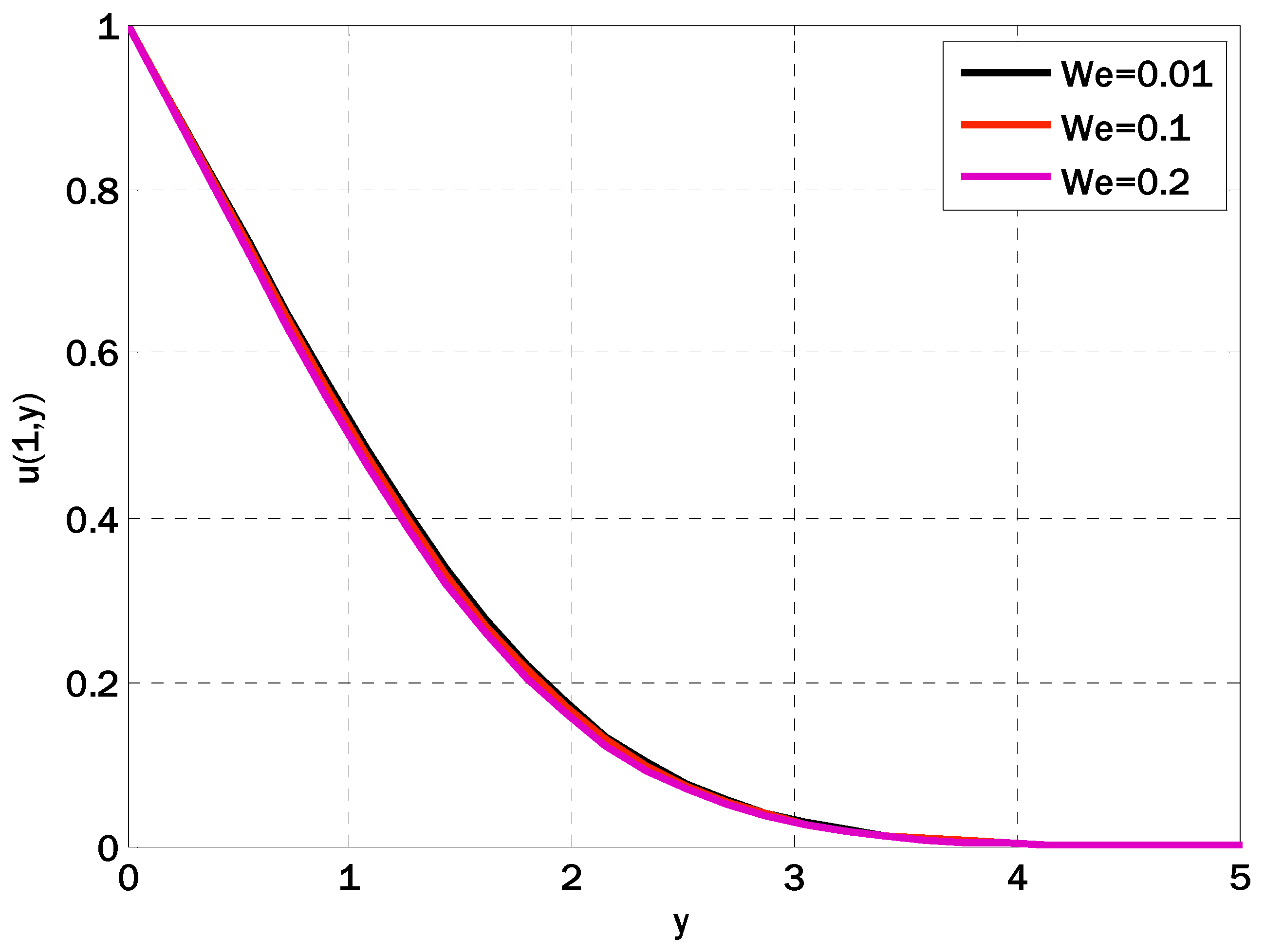
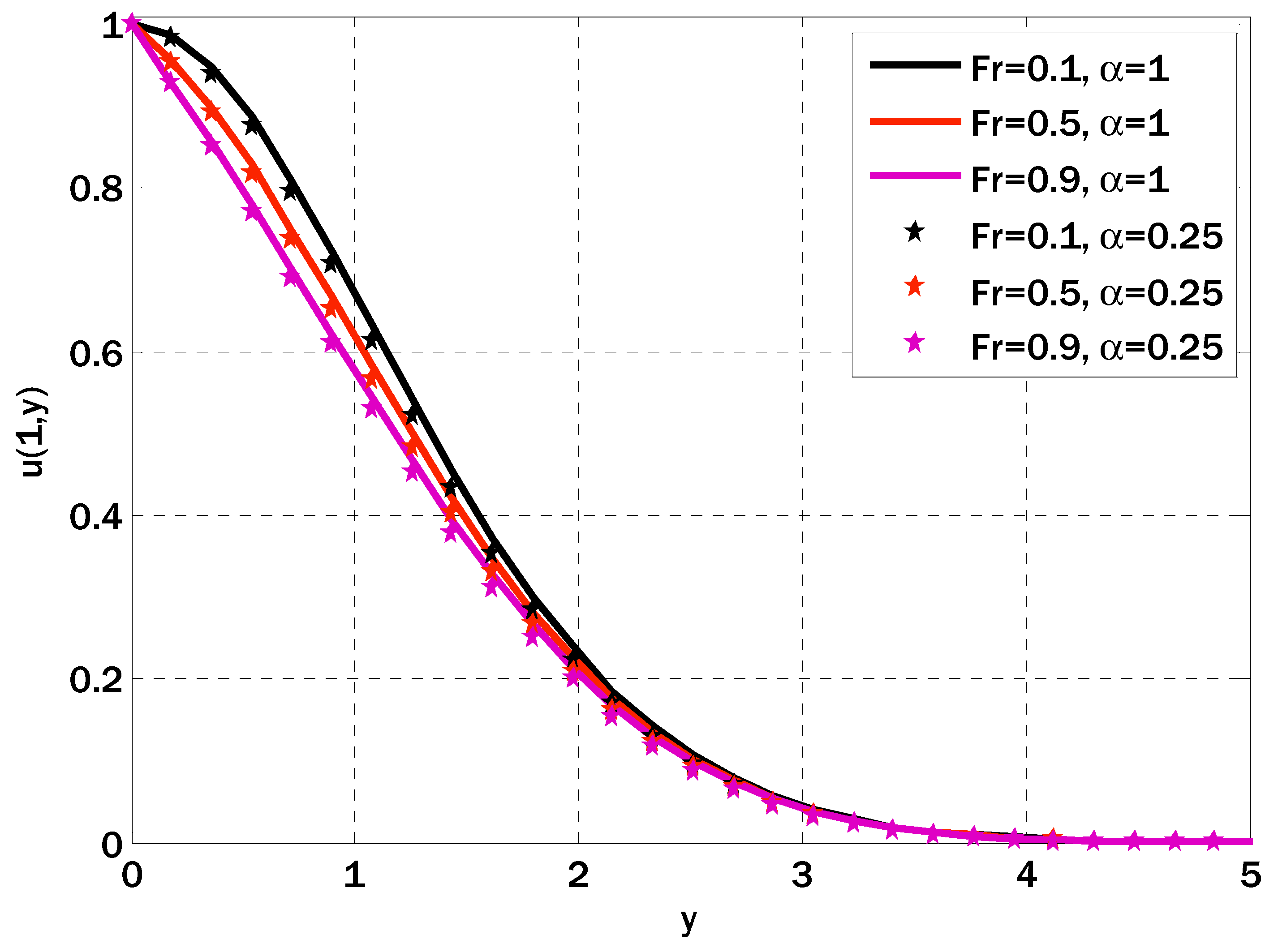
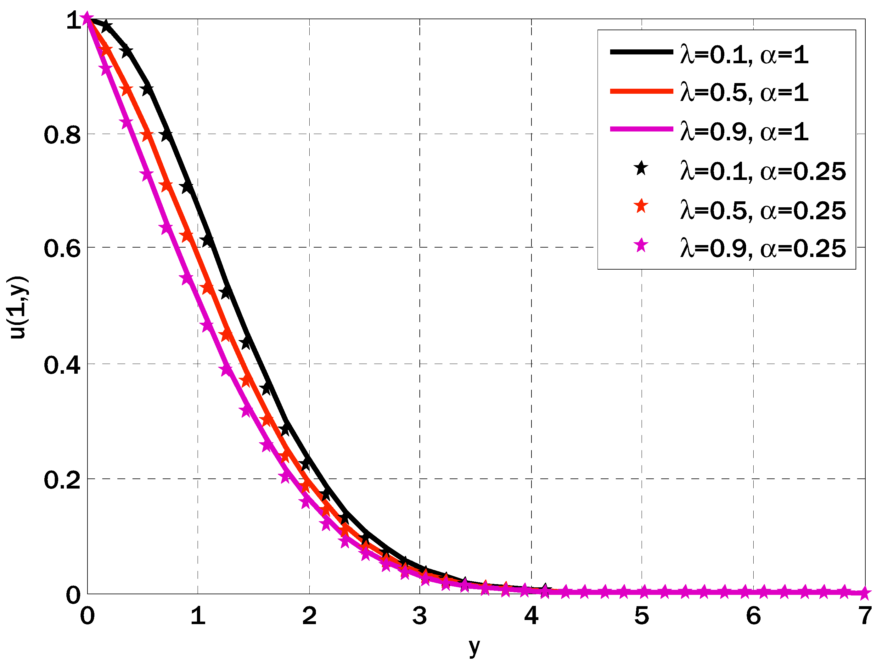
• Intensifying the magnetic field parameter, porosity parameter, inertia coefficient, and Weisenberg number decreased the velocity profile.
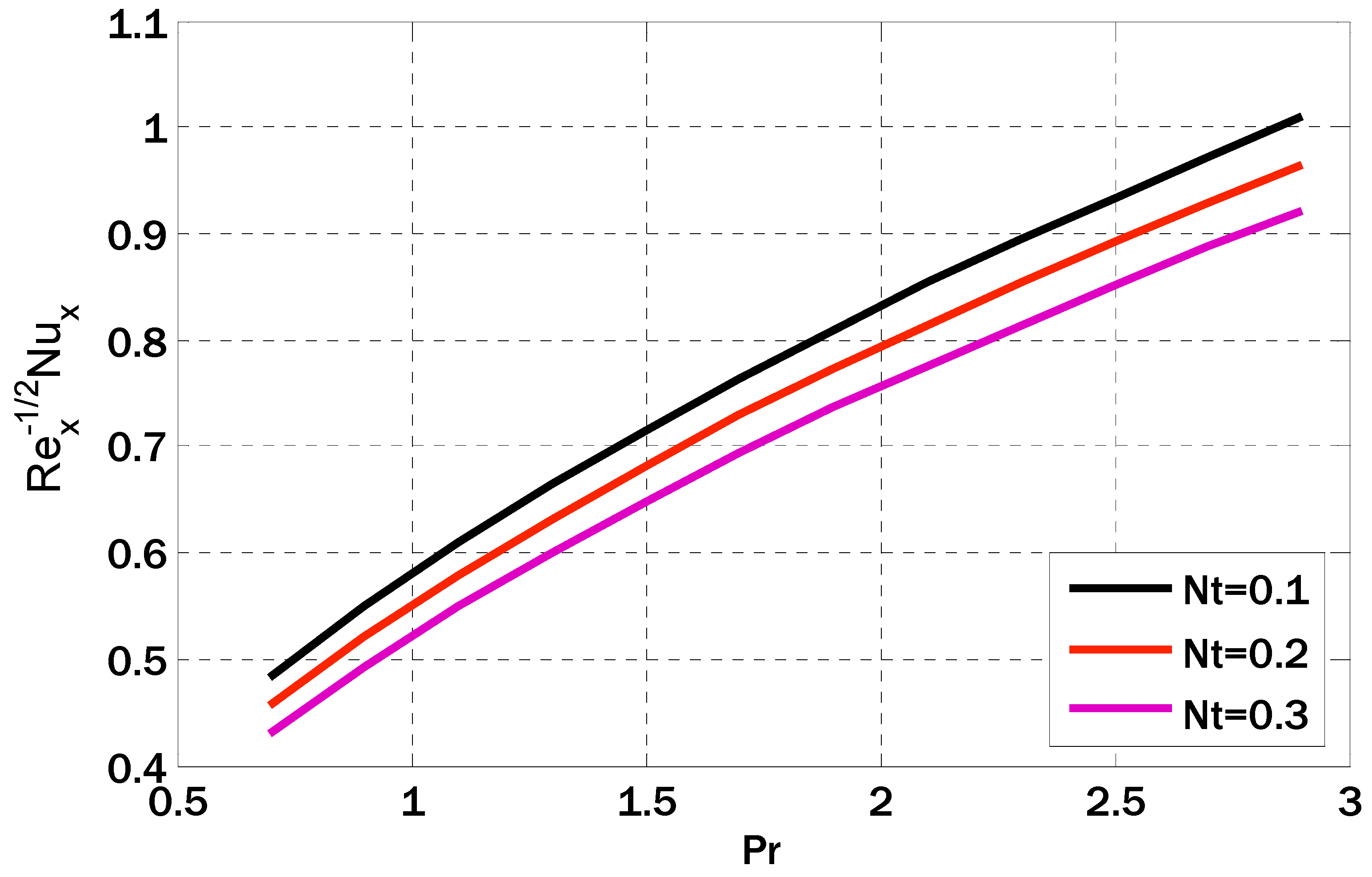
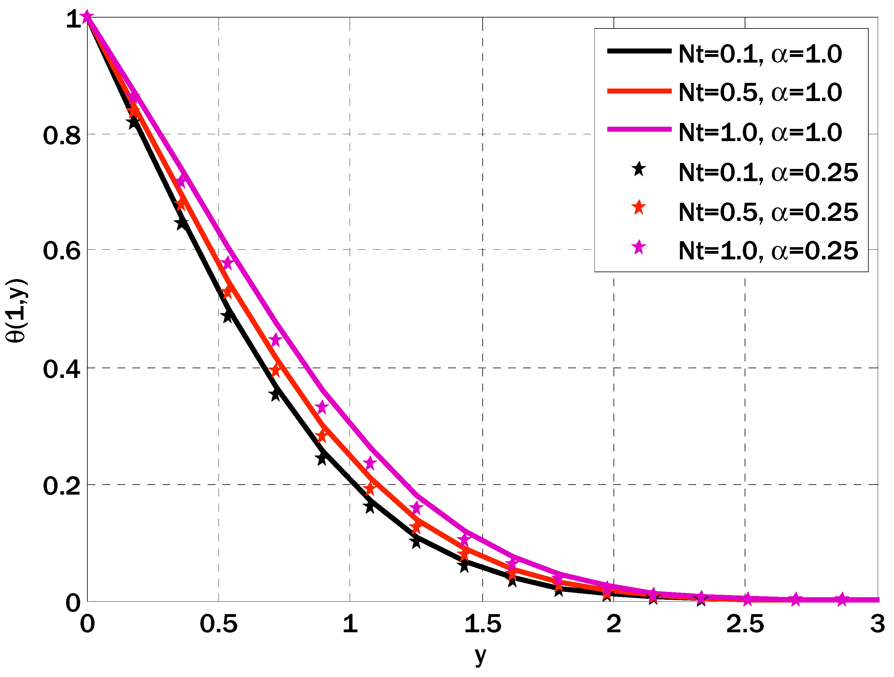
• The temperature profile increased when the Brownian motion parameter values and thermophoresis parameters were increased.
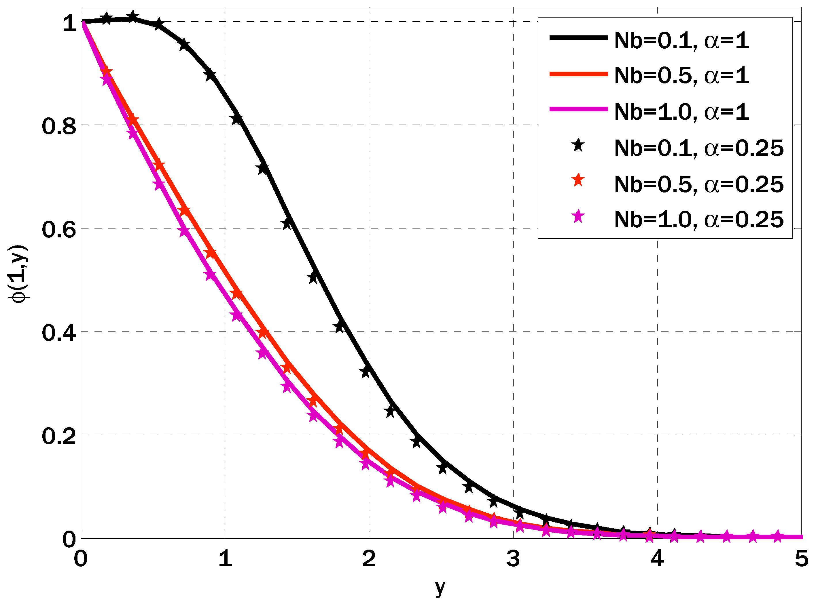
• As the value of the Brownian motion parameter increased, the concentration profile dipped.

Many problems involving the motion of non-Newtonian nanofluids through magnetic fields and porous media can be investigated with the help of the proposed numerical scheme. The research findings can enhance the development of nanofluid-based technologies for various uses. Besides shear-thinning and shear-thickening nanofluids, the suggested numerical scheme can be utilized to investigate the flow of various non-Newtonian nanofluids. These fluids’ flow behavior and potential uses could be better understood in this way. Nanofluid flow in more complicated geometries like curved channels and pipelines can be studied with the suggested numerical scheme. This would help us learn more about how nanofluids behave in practical settings.

References

1. Choi, S.U.S.; Eastman, J.A. Enhancing Thermal Conductivity of Fluids with Nanoparti-Cles; ASME International Mechanical Engineering Congress & Exposisition; American Society of Mechanical Engineers: San Francisco, FL, USA, 1995; Volume 66, pp. 99–105. [Google Scholar]
2. Rasool, G.; Zhang, T. Characteristics of chemical reaction and convective boundary conditions in Powell-Eyring nanofluid flow along a radiative Riga plate. Heliyon 2019, 5, e01479. [Google Scholar] [CrossRef] [PubMed]
3. Bai, Y.; Liu, X.; Zhang, Y.; Zhang, M. Stagnation-point heat and mass transfer of MHD Maxwell nanofluids over a stretching surface in the presence of thermophoresis. J. Mol. Liq. 2016, 224, 1172–1180. [Google Scholar] [CrossRef]
4. Jusoh, R.; Nazar, R.; Pop, I. Flow and heat transfer of magneto-hydrodynamic three-dimensional Maxwell nanofluid over a permeable stretching/shrinking surface with convective boundary conditions. Int. J. Mech. Sci. 2018, 124, 166–173. [Google Scholar]
5. Dogonchi, A.S.; Chamkha, A.J.; Ganji, D.D. A numerical investigation of magneto-hydrodynamic natural convection of Cu-water nanofluid in a wavy cavity using CVFEM. J. Therm. Anal. Calorim. 2019, 135, 2599–2611. [Google Scholar] [CrossRef]
6. Sakiadis, B.C. Boundary-layer behavior on continuous solid surfaces: Boundary-layer equations for two-dimensional and axisymmetric flow. AIChE J. 1961, 7, 26–28. [Google Scholar] [CrossRef]
7. Crane, L.J. Flow past a stretching plate. Angew. Math. Phys. 1970, 21, 645. [Google Scholar] [CrossRef]
8. Rasool, G.; Shafiq, A.; Khalique, C.M.; Zhang, T. Magneto-hydrodynamic Darcy Forchheimer nanofluid flow over nonlinear stretching sheet. Phys. Scr. 2019, 94, 105221. [Google Scholar] [CrossRef]
9. Rasool, G.; Zhang, T. Darcy-Forchheimer nanofluidic flow manifested with Cattaneo-Christov theory of heat and mass flux over nonlinearly stretching surface. PLoS ONE 2019, 14, e0221302. [Google Scholar] [CrossRef]
10. Sandeep, N.; Sulochana, C.; Kumar, B.R. UnsteadyMHDradiative flow and heat transfer of a dusty nanofluid over an exponentially stretching surface. Eng. Sci. Technol. 2016, 19, 227–240. [Google Scholar]
11. Hayat, T.; Qayyum, S.; Alsaedi, A.; Shafiq, A. Inclined magnetic field and heat source/sink aspects in flow of nanofluid with nonlinear thermal radiation. Int. J. Heat Mass Transf. 2016, 103, 99–107. [Google Scholar] [CrossRef]
12. Ziaei-Rad, M.; Saeedan, M.; Afshari, E. Simulation and prediction of MHD dissipative nanofluid flow on a permeable stretching surface using artificial neural network. Appl. Therm. Eng. 2016, 99, 373–382. [Google Scholar] [CrossRef]
13. Williamson, R.V. The flow of pseudoplastic materials. Ind. Eng. Chem. 1929, 21, 1108–1111. [Google Scholar] [CrossRef]
14. Blasius, H. The Boundary Layers in Fluids with Little Friction; NACA: Washington, DC, USA, 1950. [Google Scholar]
15. Ramesh, G.K.; Gireesha, B.J.; Gorla, R.S.R. Study on Sakiadis and Blasius flows of Williamson fluid with convective boundary condition. Nonlinear Eng. 2015, 4, 215–221. [Google Scholar] [CrossRef]
16. Khan, M.; Malik, M.Y.; Salahuddin, T.; Rehman, K.U.; Naseer, M.; Khan, I. MHD flow of Williamson nanofluid over a cone and plate with chemically reactive species. J. Mol. Liq. 2017, 231, 580–588. [Google Scholar] [CrossRef]
17. Hayat, T.; Bashir, G.; Waqas, M.; Alsaedi, A. MHD 2D flow ofWilliamson nanofluid over a nonlinear variable thicked surface with melting heat transfer. J. Mol. Liq. 2016, 223, 836–844. [Google Scholar] [CrossRef]
18. Nadeem, S.; Hussain, S.T.; Lee, C. Flow of aWilliamson fluid over a stretching sheet. Braz. J. Chem. Eng. 2013, 30, 619–625. [Google Scholar] [CrossRef]
19. Salahuddin, T.; Malik, M.Y.; Hussain, A.; Bilal, S.; Awais, M. MHD Flow of Cattanneo-Christov heat flux model for Williamson fluid over a stretching sheet with variable thickness: Using numerical approach. J. Magn. Magn. Mater. 2016, 401, 991–997. [Google Scholar] [CrossRef]
20. Hayat, T.; Saeed, Y.; Asad, S.; Alsaedi, A. Soret and Dufour effects in the flow ofWilliamson fluid over an unsteady stretching surface with thermal radiation. Z. Naturforschung A 2015, 70, 235–243. [Google Scholar] [CrossRef]
21. Buongiorno, J. Convective transport in nanofluids. J. Heat Transfer. 2006, 128, 240–250. [Google Scholar] [CrossRef]
22. Tiwari, R.K.; Das, M.K. Heat transfer augmentation in a two sided lid-driven differentially heated square cavity utilizing nanofluid. Int. J. Heat Mass Transf. 2007, 50, 2002–2018. [Google Scholar] [CrossRef]
23. Makinde, O.D.; Chinyoka, T. MHD transient flows and heat transfer of dusty fluid in a channel with variable physical properties and Navier slip condition. Comput. Math. Appl. 2010, 60, 660–669. [Google Scholar] [CrossRef]
24. Jalilpour, B.; Jafarmadar, S.; Rashidi, M.M.; Ganji, D.D.; Rahime, R.; Shotorban, A.B. MHD non-orthogonal stagnation point flow of a nanofluid towards a stretching surface in the presence of thermal radiation. Ain Shams Eng. J. 2017, 9, 1671–1681. [Google Scholar] [CrossRef]
25. Sandeep, N. Effect of aligned magnetic field on liquid thin film flow of magnetic-nanofluids embedded with graphene nanoparticles. Adv. Powder Technol. 2017, 28, 865–875. [Google Scholar] [CrossRef]
26. Sucharitha, G.; Lakshminarayana, P.; Sandeep, N. Joule heating and wall flexibility effects on the prristaltic flow of magneto-hydrodynamic nanofluid. Int. J. Mech. Sci. 2017, 131–132, 52–62. [Google Scholar] [CrossRef]
27. Nadeem, S.; Hussain, S.T. Flow and heat transfer analysis of Williamson nanofluid. Appl. Nanosci. 2014, 4, 1005–1012. [Google Scholar] [CrossRef]
28. Krishnamurthy, M.R.; Prasannakumara, B.C.; Gireesha, B.J.; Gorla, R.S.R. Effect of chemical reaction on MHD boundary layer flow and melting heat transfer of Williamson nanofluid in porous medium. Eng. Sci. Technol. Int. J. 2016, 19, 53–61. [Google Scholar] [CrossRef]
29. Forchheimer, P. Wasserbewegung durch boden. Z. Ver. Dtsch. Ing. 1901, 45, 1782–1788. [Google Scholar]
30. Muskat, M.; Meres, M.W. The flow of heterogeneous fluids through porous media. Physics 1936, 7, 346–363. [Google Scholar] [CrossRef]
31. Sadiq, M.A.; Hayat, T. Darcy-Forchheimer flow of magneto Maxwell liquid bounded by convectively heated sheet. Results Phys. 2016, 6, 884–890. [Google Scholar] [CrossRef]
32. Khan, A.; Shah, Z.; Islam, S.; Khan, S.; Khan, W.; Khan, A.Z. Darcy-Forchheimer flow of micropolar nanofluid between two plates in the rotating frame with non-uniform heat generation/absorption. Adv. Mech. Eng. 2018, 10, 1–16. [Google Scholar] [CrossRef]
33. Hayat, T.; Haider, F.; Muhammad, T.; Alsaedi, A. Darcy-Forchheimer flow due to a curved stretching surface with Cattaneo-Christov double diffusion: A numerical study. Results Phys. 2017, 7, 2663–2670. [Google Scholar] [CrossRef]
34. Muhammad, T.; Rafique, K.; Asma, M.; Alghamdi, M. Darcy-Forchheimer flow over an exponentially stretching curved surface with Cattaneo-Christov double diffusion. Phys. A 2019, 556, 123968. [Google Scholar] [CrossRef]
35. Hayat, T.; Saif, R.S.; Ellahi, R.; Muhammad, T.; Ahmad, B. Numerical stuy for Darcy-Forchheimer flow due to a curved stretching surface with Cattaneo-Christov heat flux and homogeneous-hetrogeneous reactions. Results Phys. 2017, 7, 2886–2892. [Google Scholar] [CrossRef]
36. Rasool, G.; Zhang, T.; Chamkha, A.J.; Shafiq, A.; Tlili, I.; Shahzadi, G. Entropy generation and consequences of binary chemical reaction on MHD Darcy–Forchheimer Williamson Nanofluid flow over nonlinearly stretching surface. Entropy 2020, 22, 18. [Google Scholar] [CrossRef] [PubMed]
37. Khan, Z.A.; Shah, K.; Abdalla, B.; Abdeljawad, T. A numerical Study of Complex Dynamics of a Chemostat Model Under Fractal-Fractional Derivative. Fractals 2023, 31, 2340181. [Google Scholar] [CrossRef]
38. Sana, G.; Mohammed, P.O.; Shin, D.Y.; Noor, M.A.; Oudat, M.S. On iterative methods for solving nonlinear equations in Quantum calculus. Fractal Fract. 2021, 5, 60. [Google Scholar] [CrossRef]
39. Nawaz, Y.; Arif, M.S.; Abodayeh, K. An explicit-implicit numerical scheme for time fractional boundary layer flows. Int. J. Numer. Methods Fluids 2022, 94, 920–940. [Google Scholar] [CrossRef]
40. Nawaz, M.; Adil Sadiq, M. Unsteady heat transfer enhancement in Williamson fluid in Darcy-Forchheimer porous medium under non-Fourier condition of heat flux. Case Stud. Therm. Eng. 2021, 28, 101647. [Google Scholar] [CrossRef]
41. Kho, Y.B.; Hussanan, A.; Mohamed, M.K.A.; Salleh, M.Z. Heat and mass transfer analysis on flow of Williamson nanofluid with thermal and velocity slips: Buongiorno model. Propuls. Power Res. 2019, 8, 243–252. [Google Scholar] [CrossRef]
42. Nawaz, Y.; Arif, M.S.; Abodayeh, K. A Compact Numerical Scheme for the Heat Transfer of Mixed Convection Flow in Quantum Calculus. Appl. Sci. 2022, 12, 4959. [Google Scholar] [CrossRef]
Figure 1. Comparison of the fractal proposed and the fractal Crank–Nicolson schemes for finding norm over consumed iterations using α = 0.25 ,   W e = 0.1 ,   λ = 0.1 ,   F r = 0.1005 ,   M = 0.1 ,   λ 1 = 0.5 ,   λ 2 = 0.7 ,   P r = 3 ,   N b = 0.3 ,   N t = 0.1 ,   S c = 1 ,   γ = 0.2 ,   q = 0.7 .
Fractalfract 08 00008 g001
Figure 2. Effect of variation in Weisenberg number on velocity profile using α = 1 , λ = 0.1 , F r = 0.1 , M = 0.9 , λ 1 = 0.5 , λ 2 = 0.7 , P r = 3 , N b = 0.1 , N t = 0.1 , S c = 1 , γ = 0.1 , q = 0.7 .
Fractalfract 08 00008 g002
Figure 3. Effect of variation in magnetic field parameter on velocity profile using λ = 0.1 , F r = 0.1 , W e = 0.1 , λ 1 = 0.5 , λ 2 = 0.7 , P r = 3 , N b = 0.1 , N t = 0.1 , S c = 1 , γ = 0.1 , q = 0.7 .
Fractalfract 08 00008 g003
Figure 4. Effect of variation in porosity parameter on velocity profile using M = 0.1 , F r = 0.1 , W e = 0.1 , λ 1 = 0.5 , λ 2 = 0.7 , P r = 3 , N b = 0.1 , N t = 0.1 , S c = 1 , γ = 0.1 , q = 0.7 .
Fractalfract 08 00008 g004
Figure 5. Effect of variation in inertia coefficient on velocity profile using  M = 0.1 , λ = 0.1 , W e = 0.1 , λ 1 = 0.5 , λ 2 = 0.7 , P r = 3 , N b = 0.1 , N t = 0.1 , S c = 1 , γ = 0.1 , q = 0.7 .
Fractalfract 08 00008 g005
Figure 6. Effect of variation in Brownian motion parameter on temperature profile using  M = 0.1 , λ = 0.1 , W e = 0.1 , λ 1 = 0.5 , λ 2 = 0.7 , P r = 3 , F r = 0.1 , N t = 0.1 , S c = 1 , γ = 0.1 , q = 0.7 .
Fractalfract 08 00008 g006
Figure 7. Effect of variation in thermophoresis parameter on temperature profile using  M = 0.1 , λ = 0.1 , W e = 0.1 , λ 1 = 0.5 , λ 2 = 0.7 , P r = 3 , F r = 0.1 , N b = 0.1 , S c = 1 , γ = 0.1 , q = 0.7 .
Fractalfract 08 00008 g007
Figure 8. Effect of variation in Brownian motion parameter on concentration profile using  M = 0.1 , λ = 0.1 , W e = 0.1 , λ 1 = 0.5 , λ 2 = 0.7 , P r = 3 , F r = 0.1 , N t = 0.1 , S c = 1 , γ = 0.1 , q = 0.7 .
Fractalfract 08 00008 g008
Figure 9. Effect of variation in Weisenberg number and inertia coefficient on skin friction coefficient using  α = 0.25 ,   M = 0.1 ,   λ = 0.1 ,   λ 1 = 0.5 ,   λ 2 = 0.7 ,   P r = 3 ,   N t = 0.1 ,   N b = 0.1 ,   S c = 1 ,   γ = 0.1 ,   q = 0.7 .
Fractalfract 08 00008 g009
Figure 10. Effect of variation in Prandtl number and thermophoresis parameter on local Nusselt number using  α = 0.25 , M = 0.1 , λ = 0.1 , λ 1 = 0.5 , λ 2 = 0.7 , W e = 0.1 , F r = 0.1005 , N b = 0.1 , S c = 1 , γ = 0.1 , q = 0.7 .
Fractalfract 08 00008 g010
Figure 11. Effect of variation in Schmidt number and reaction rate parameter on local Sherwood number using  α = 0.25 , M = 0.1 , λ = 0.1 , λ 1 = 0.5 , λ 2 = 0.7 , W e = 0.1 , F r = 0.1005 , N b = 0.1 , P r = 3 , N t = 0.1 , q = 0.7 .
Fractalfract 08 00008 g011
Figure 12. Contour plot for velocity profile using  α = 0.25 , M = 0.1 , λ = 0.1 , λ 1 = 0.5 , λ 2 = 0.7 , W e = 0.1 , F r = 0.1005 , N b = 0.3 , P r = 3 , N t = 0.1 , q = 0.7 , S c = 1 , γ = 0.2 , L ( l e n g t h   o f   d o n m a i n ) = 17 , u w = s i n t + c o s t .
Fractalfract 08 00008 g012
Figure 13. Contour plot for velocity profile using  α = 0.25 , M = 0.1 , λ = 0.1 , λ 1 = 0.5 , λ 2 = 0.7 , W e = 0.1 , F r = 0.1005 , N b = 0.3 , P r = 3 , N t = 0.1 , q = 0.7 , S c = 1 , γ = 0.2 , L ( l e n g t h   o f   d o n m a i n ) = 17 , u w = s i n t c o s t .
Fractalfract 08 00008 g013
Figure 14. Mesh plot for velocity profile using  α = 0.25 , M = 0.1 , λ = 0.1 , λ 1 = 0.5 , λ 2 = 0.7 , W e = 0.1 , F r = 0.1005 , N b = 0.3 , P r = 3 , N t = 0.1 , q = 0.7 , S c = 1 , γ = 0.2 , L ( l e n g t h   o f   d o n m a i n ) = 17 , u w = s i n t + c o s t .
Fractalfract 08 00008 g014
Figure 15. Mesh plot for velocity profile using  α = 0.25 , M = 0.1 , λ = 0.1 , λ 1 = 0.5 , λ 2 = 0.7 , W e = 0.1 , F r = 0.1005 , N b = 0.3 , P r = 3 , N t = 0.1 , q = 0.7 , S c = 1 , γ = 0.2 , L ( l e n g t h   o f   d o n m a i n ) = 17 , u w = s i n t c o s t .
Fractalfract 08 00008 g015
Figure 16. Comparison of the exact and numerical solutions and also the effect of  q  for velocity profile using  α = 1 ,   M = 0 ,   λ = 0 ,   λ 1 = 0 ,   λ 2 = 0 ,   W e = 0 ,   u w = 1 .
Fractalfract 08 00008 g016