Abstract
In this study, a nonlinear Archimedes wave swing (AWS) energy conversion system was employed to enable the use of irregular sea waves to provide useful electricity. Instead of the conventional PI controllers used in prior research, this study employed fractional-order PID (FOPID) controllers to control the back-to-back configuration of AWS. The aim was to maximize the energy yield from waves and maintain the grid voltage and the capacitor DC link voltage at predetermined values. In this study, six FOPID controllers were used to accomplish the control goals, leading to an array of thirty parameters required to be fine-tuned. In this regard, a hybrid jellyfish search optimizer and particle swarm optimization (HJSPSO) algorithm was adopted to select the optimal control gains. Verification of the performance of the proposed FOPID control system was achieved by comparing the system results to two conventional PID controllers and one FOPID controller. The conventional PID controllers were tuned using a recently presented metaheuristic algorithm called the Coot optimization algorithm (COOT) and the classical particle swarm optimization algorithm (PSO). Moreover, the FOPID was also tuned using the well-known genetic algorithm (GA). The system investigated in this study was subjected to various unsymmetrical and symmetrical fault disturbances. When compared with the standard COOT-PID, PSO-PID, and GA-FOPID controllers, the HJSPSO-FOPID results show a significant improvement in terms of performance and preserving control goals during system instability
1. Introduction
1.1. Background and Motivation
Wave energy is one of the most abundant renewable energy resources that can provide enough energy to satisfy the world’s needs. According to the World Energy Council, wave energy has an estimated energy of 17.5 PWh/year, which is more than enough to fill the estimated energy requirements of 16 PWh/year globally [1]. The benefits of using wave energy include avoiding the need for expensive real estate, and a short distance between wave energy converters and consumption because a large portion of the world lives on the ocean’s shores, resulting in lower energy losses; lower investment in transmission lines; and higher power density compared with other renewable resources, such as wind and solar energies. Therefore, a large interest has developed toward convert wave energy into electricity, which led to the invention of numerous wave energy converters, like the Oscillating Water Column, Archimedes Wave Swing (AWS), Wave Dragon, Pelamis Wave Power, Aquabouy, and the Oyster [2]. The AWS converter was chosen by the authors for use in this study because it is one of the most regularly used converters and is employed by a well-known company (AWS Ocean Energy) [3,4].
For the AWS, two models were adopted in the literature, namely, the linear and nonlinear models. The linear model is the AWS simplified version that was built by Polinder during an experiment involving AWS in Portugal [5]. Since this version of AWS modeling is based on an experiment with limitations on the generated power and many forces were neglected for simplicity, a higher-order nonlinear model was needed for more accurate results.
Numerous studies emphasized the importance of employing nonlinear models to achieve precision in computational outcomes. For instance, a study presented in [6] developed a high-order and efficient numerical technique that was specifically designed for solving the nonlocal neutron diffusion equation, which models neutron transport within a nuclear reactor. In a separate investigation detailed in [7], an -norm error analysis of a robust ADI method on graded meshes was conducted to address three-dimensional subdiffusion problems. Furthermore, another study [8] examined the preservation of positivity in a nonlinear finite volume method tailored for multi-term fractional subdiffusion equations, particularly on polygonal meshes. These nonlinear models are crucial for understanding reactor behavior and optimizing reactor performance in various applications.
For the AWS, the time domain model of AWS was first introduced in [9] without any practical values that can help build this model. Then, nonlinear model equations were provided by Gieske in [10], along with the parameters’ values of the system. Then, the same equations with a grid-connected system and a control system suitable for this nonlinear system were introduced by the authors of this work [11]. This model was used in this study.
1.2. Literature Overview
A review of the control systems for AWS in the literature is helpful for comprehending the contribution of this work fully. The first control strategy is the conventional PID controller; this controller is adopted in many research works with different optimization algorithms used. For example, in [12], Feng introduced how to obtain the maximum energy from waves using dq current control with PI controllers. In [13], the water cycle algorithm (WCA) [14] was employed to select the gains of six PI controllers to maximize the energy harvest and maintain the DC link capacitor voltage and the voltage at the point of connection with the grid (point of common coupling) () at the reference values. This system required six conventional PI controllers. The results of this work were compared with the genetic algorithm (GA), which showed a much better response. In [15], the Coot optimization algorithm (COOT) [16] was employed to tune the same controllers. In addition, an anti-windup technique that damps the overshooting of due to the integrator part of the PI controller was added. The results of this algorithm were compared with six other recent algorithms. The conclusion was that the addition of the anti-windup technique enhanced the system’s transient behavior.
Similarly, in [17], the salp swarm algorithm [18] was employed to find the optimal gains of the PI controllers, and the system behavior was observed in the presence of irregular waves. In [19], a supercapacitor with a bidirectional converter was connected in parallel to a DC link to provide constant power to the grid. In [20], the supercapacitor technique was also employed in a hybrid wave–solar power plant to provide constant power to a version three (V3) supercharging station that charges Tesla cars. The golden jackal algorithm [21] tuned the gains of the controllers. Alongside the supercharging station, which is related to the DC microgrid, several research works involved the DC grid. For instance, in [22], the gravitational search algorithm [23] was employed to set the optimal gains of three PI controllers that achieved a successful connection to the DC grid. The gravitational search results were compared with the GA during fault conditions. In [11], the six PI controllers were tuned using the hybrid augmented grey wolf optimizer and cuckoo search (AGWO-CS) algorithm [24]. The results were compared with PI controllers optimized using COOT and PSO during different grid faults. Moreover, OP4510, along with the RT-Lab program, was employed to conduct a real-time simulation of the AWS system to experimentally validate the accuracy of results. Other than the PID controllers, other techniques were implemented. For example, in [10,25], a model predictive control was employed for the generator-side converter to maximize energy harvesting. For the same objective, neural network models were established in [26], along with different control strategies.
1.3. Objectives and Contributions
Our main objective was to implement a control strategy that had not been employed before for the nonlinear AWS grid-connected system. In this regard, we investigated adopting a fractional-order PID (FOPID) in the back–back configuration controllers as a replacement for the conventional PID adopted in the literature for AWS. The FOPID controllers have several merits compared with the conventional PID controllers. For example, the presence of fractional orders in the integrator and differentiator provides more flexible tuning (extra degrees of freedom) that leads to more stability and robustness in highly nonlinear systems, like AWS. Furthermore, as will be proven in this work, the FOPID controllers lead to a better response of the system and reduced overshooting during transient states. Moreover, the FOPID controllers could lead to lower energy consumption as a result of their fine-tuning control action, as in [27]. Additionally, the FOPID controllers were employed in different renewable energy resources, like wind energy [28], solar energy [29], fuel cells [30], and hydroelectric [31]. In addition, the FOPID control strategy was utilized in the speed control of a PMSM [32]. Furthermore, the control of an automatic voltage regulator using FOPID was achieved in [33,34]. Also, improved frequency controllers based on the FOPID strategy regulated the frequency of inter-connected power grids [35]. Moreover, a modified version of FOPID was used to regulate a hybrid inter-connected system formed of various renewable resources [36]. To implement the FOPID control strategy, a comprehensive understanding of the AWS connected to the power grid is mandatory. The AWS device requires a back–back converter configuration for a successful grid connection. The rectifier’s controllers minimize generator losses and generate maximum power from waves by controlling the stator dq currents. Furthermore, the inverter’s controllers ensure 1 p.u and by controlling the output dq currents of the inverter. This back–back configuration requires six fractional-order PID controllers. Each one requires five gains to be tuned using a powerful algorithm. In this work, a hybrid algorithm formed from the jellyfish search optimizer and particle swarm optimization (HJSPSO) was employed [37]. The HJSPSO is a hybrid algorithm that takes advantage of the exploitation ability of the jellyfish optimizer (JO) [38] in addition to the exploration advantage of the particle swarm optimization algorithm (PSO) [39]. The results were compared with two conventional PID controllers that were optimized using the PSO [39] and COOT [16], in addition to controllers’ gains that were tuned using the GA.
The work’s main contributions are summarized as follows:
- A thorough mathematical modeling of the grid-connected AWS, including the back-to-back converter controllers, is presented, together with all of the system’s parameter values.
- The proposed FOPID controllers, the number of gains that must be tuned, and the HJSPSO method utilized for selecting the best gains are all detailed.
- The HJSPSO-FOPID controllers were compared with two conventional PID controllers that were tuned using PSO and COOT, in addition to FOPID controllers that were tuned using the GA.
- The controllers’ effectiveness and reliability were demonstrated by subjecting the grid-connected system to various unsymmetrical and symmetrical fault disturbances.
1.4. Organization
For a better understanding of this work, it was divided into multiple sections. In the Section 2, the modeling of the nonlinear AWS with detailed equations and parameters’ values is presented. In the Section 3, the grid-connected system with the inverter and rectifier in addition to the control system is elaborated. Furthermore, the FOPID controller strategy is explained. In the Section 4, the optimization algorithm of the HJSPSO, the final errors of the different algorithms, and the optimal gains are also presented. In the Section 5, the system’s results during steady and transient states and the performance of each controller are discussed in detail. Finally, the Section 6, namely, the conclusion section, contains a summary of this work and future work suggestions.
2. Modeling of the AWS Wave Energy Conversion System
The wave energy conversion device consists of a floater that moves upward and downward due to the pressure variation on the floater due to the wave crest and trough. The floater’s motion generates electricity by employing a linear synchronous generator that converts the vertical motion into three-phase output power. This work adopts the nonlinear version of the AWS explained in [8]. The general expression for the nonlinear model is formulated as follows:
In these equations, the velocity of the floater and the current floater position are denoted by and , respectively. The gravitational force () and the drag force of water () are mathematically represented as follows:
is the gravitational force pushing the device’s floater downward. This force relies on the mass of the floater () and the gravitational acceleration (), whereas represents the opposite force acting from the fluid (water) against the motion of the floater. This force is controlled by the outer area of the device floater (), , and the seawater density (), in addition to the upward drag coefficient () during the positive velocity and downward coefficient () during the negative velocity. Moreover, in the model’s main equation, we have the end force () exerting a large force when the floater hits an end position (), after which the floater will be damaged. The spring force () that returns the floater to the equilibrium position when no waves are available. The water brakes’ force () acts when a certain vertical violation is reached. These forces are represented as follows:
In the previous formulas, the end position, the added mass, and the applied force of the spring at the equilibrium position () at which all of the forces cancel each other, the spring length at equilibrium, the hydrostatic force at equilibrium, the angular tuning frequency, the heat capacity rate, the position at which the brakes will be activated, and the brakes’ coefficient are all denoted by , , , , , , , , and , respectively. The radiation force () represents a load on the floater when new radiated waves are created due to the floater’s motion, the hydrostatic force represents the force affecting the AWS floater due to the pressure of seawater, and the approximated radiation force adopted () are expressed as follows [5,10]:
where the fluid’s retardation function, the ambient pressure, the tide level, the inner crossectional area of the floater, the depth at mid-position, and the height of the floater are denoted by , , , , , and . is very difficult to calculate precisely, and thus, the expressions obtained by Gieske in (11) and (12) are adopted [10].
Furthermore, the approximated excitation forces of sea waves () and the generator force () can be expressed as follows:
In the previous equations, the elevation of the resultant sea waves, the wave number, the sea depth, the current depth, the wave decay factor, the elevation of each wave, the phase shift, the angular frequency, the frequency interval, the peak energy density period, the significant wave height of the irregular waves, the spectral density, the wave amplitude, the number of waves, the generator power, the flux linkage of the permanent magnets of the linear generator’s translator, the quadrature axis current, and the stator angular frequency are symbolized by , , , , , , , , , , , , respectively.
The generated elevation of sea waves and the corresponding excitation force based on the Bretschneider spectrum is shown in Figure 1 [40].
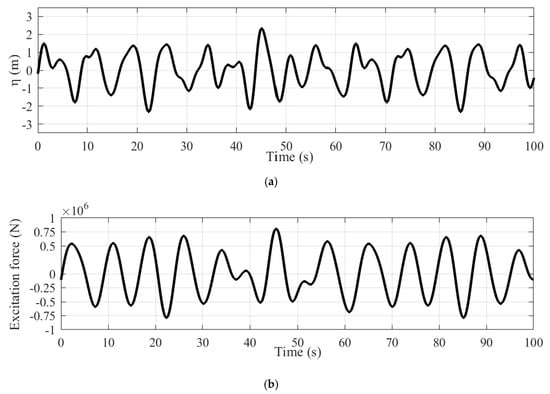
Figure 1.
(a) Resultant elevation () and (b) excitation force of waves ().
To understand the expression of , we need to obtain the generated three-phase terminal voltage () during the positive and negative velocities of the floater. is expressed as follows [15]:
where the three-phase flux linkage, the self-inductance, the mutual inductance, the inductance matrix, and the resistance of the three-phase system are symbolized by , , , and .
In addition, the generator dq axis model for controlling the AWS during both the positive and negative motion of the floater is mandatory. This expression can be obtained by applying Park’s transformation to the three-phase voltages during both motions. The Park’s transformation and the dq currents during both motions are expressed as follows [41]:
where the linear generator dq and voltages are symbolized by , , , and . Moreover, the synchronous reactance, the width of the generator pole, and the transformation angle from the abc frame to the dq frame are denoted by (), , and ( = 2πx/λ − π/2), respectively.
Finally, the frictional bearing force () due to the friction in the bearings of the floater as a result of the applied horizontal force of waves () on the AWS floater bearings is expressed as follows:
where , , μ, , , and represent the drag coefficient of water, the outer diameter of the floater, the friction coefficient, the inertia coefficient, the horizontal velocity of waves, and the horizontal acceleration of the waves. To sum up, the values of all the nonlinear model coefficients are shown in Table 1 [10,11].

Table 1.
The values of the model parameters.
3. The Grid-Connected System: Block Diagram
The AWS-generated real power is transferred to the power grid via a back–back converter configuration formed of a rectifier and an inverter. The output of the grid-side inverter is filtered using a series RL filter, after which the output will be provided to a power transformer that increases the output voltage to the grid level. Then, the transformer’s output is linked to the electrical grid via two parallel transmission lines. The overall system’s parameters are listed in Table 2 and the grid-connected system block diagram is depicted in Figure 2.
Table 2.
The grid-connected system values.
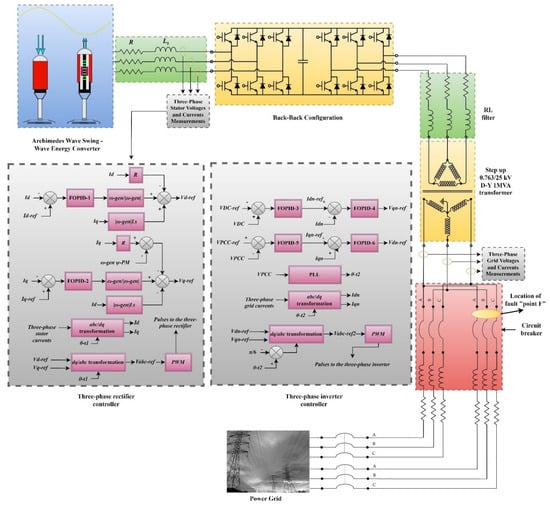
Figure 2.
The grid-connected system block diagram.
3.1. The Fractional PID (FOPID) Control Strategy
The FOPID controller is considered one of the applications of fractional calculus. This controller is considered an enhanced, extended, and generalized form of the well-known linear PID controller. The FOPID can be mathematically formulated as follows [42,43]:
The proportional, integral, and derivative gains are denoted by , , and , respectively. Furthermore, the integrator’s fractional order and the derivative’s fractional order are denoted by and , respectively. Those fractional order values are selected between 0 and 2 [44]. To obtain the conventional linear PID controller, and are set to 1.
3.2. The Back-to-Back Converter Configuration
The back-to-back converter configuration that is used to establish a successful connection with the grid is achieved by using a rectifier connected to a DC link and then connected to an inverter. The control loops for the rectifier and inverter are shown in Figure 2.
The rectifier’s controllers produce the utmost power from sea waves by maintaining the linear generator’s dq currents at the reference currents and [11]:
The required control signals are provided by two FOPID controllers that comprise the errors of these dq currents as the input. By using the Park transformation and comparing the reference with a 1 kHz triangular waveform, the required pulses are given to the six IGBTs of the rectifier. For the grid-side inverter, both and are required to be maintained at 1 p.u. By using a cascaded FOPID configuration, the errors of these voltages are provided to two FOPID controllers in the outer loop that will give the reference values of the dq currents. These values are given to the inner loop consisting of two FOPID controllers that will compare the reference and actual dq currents to generate the appropriate dq voltage signals.
Similar to the rectifier, by using the Park transformation and comparing the reference with the 1 kHz triangular waveform, the required pulses are given to the six IGBTs of the inverter. Unlike the rectifier, in this control loop, the required transformation angle is provided by the phase-locked loop (PLL) by measuring the three-phase voltages at the grid side.
To sum up, the control system consists of six FOPID controllers. Each of these controllers has five control parameters that need to be tuned. This leads to a total of thirty parameters that can be represented by an array r = [r[1], r[2], m[3], r[4], r[5], …, r[30]], where r[1], r[2], r[3], r[4], and r[5] represent the five control gains of FOPID-1, where , , , , and . Similarly, the FOPID-2 gains are represented by r[6], r[7], r[8], r[9], and r[10]. Furthermore, the rest of the FOPID controllers’ gains are obtained similarly.
4. Hybrid Jellyfish Search Optimizer and Particle Swarm Optimization (HJSPSO)
The HJSPSO is a hybrid algorithm that takes advantage of the exploitation ability of the jellyfish optimizer (JO) [38], in addition to the exploration merit of the particle swarm optimization algorithm (PSO) [39]. The tuning process alternates between the two algorithms using a time control technique to find the finest solution. Moreover, the hybrid algorithm includes several coefficients that achieve consistency between exploitation and exploration. The hybrid algorithm flowchart is illustrated in Figure 3.
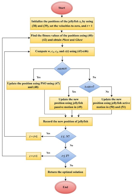
Figure 3.
The HJSPSO algorithm’s flowchart.
4.1. HJSPSO Algorithm Steps
The HJSPSO algorithm starts with the initialization of the positions of jellyfish when searching for food using the following equations:
where the ith jellyfish’s current position, the gains’ lower boundaries, the upper boundaries of the gains, the ith jellyfish’s logistic value, the initial logistic value of the jellyfish, the swarm number, and the current iteration are denoted by , , , , , and t, respectively. In addition, = 4 [37]. The fitness values of these positions are evaluated using the following equations [13]:
where the generator-side converter integral squared error of the direct axis current ) and quadrature axis current ) are denoted by . In addition, the inverter integral squared error of the , , direct axis current ), and quadrature axis current ) are combined in . Finally, these integral squared errors form the final objective function () that is adopted in MATLAB. Due to the same importance of the two controllers, the weighting factors and are set to 0.5.
To decide between the selection of PSO or JO for updating the position, the following equations are computed:
where is a random value generated by the code between zero and one and denotes the iteration number performed by the algorithm. If , then PSO is selected for updating the position as follows:
where ,, and are equal to 0.4, 0.9, 0.1, 0.5, and 2.5, respectively. Also, and are random values generated by the code in the range [0 1]. Moreover, the velocity of ith particle, the optimal personal position, and the global optimal position are denoted by , , and , respectively.
Otherwise, the JO is used to update the position. However, the JO is divided into different movements: either passive (around its current position) or active (update relative to a randomly selected jth jellyfish). The position update of the two mechanisms is expressed as follows:
where is the current swarm’s best position. The optimal values obtained using the HJSPSO for FOPID, GA for FOPID, the COOT for linear PID, and the PSO for linear PID are given in Table 3. The final errors for each algorithm after 50 iterations are shown in Figure 4.
Table 3.
The optimal controller gains.
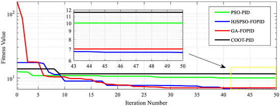
Figure 4.
The final errors for controllers.
4.2. HJSPSO Algorithm Computational Complexity
The computational complexity of an algorithm refers to the amount of resources required to execute the algorithm, such as time and memory. In the case of the HJSPSO algorithm, its computational complexity can be evaluated by measuring its execution time and comparing it with other optimization algorithms, such as PSO, COOT, and GA. The execution time of an algorithm is affected by various factors, including the size of the problem, the hardware used, and the implementation of the algorithm. The three algorithms, including COOT, PSO, and HJSPSO, had a population size of 20 and iterations of 50. The function evaluations of COOT, PSO, and HJSPSO were calculated as population size multiplied by the number of iterations, yielding a total of 1000 function evaluations. For GA, employing a population size of 15, a generation count of 50, a mutation rate set at 0.01, and a crossover rate of 0.4 were anticipated to yield evaluations closely aligned with those of other algorithms. This configuration is essential for ensuring a valid and equitable comparison between different algorithms.
When comparing the computational complexity of the HJSPSO algorithm with other optimization algorithms, such as PSO, COOT, and GA, it is essential to ensure that the comparison is valid by executing the algorithms on the same hardware specifications. The comparative analysis involved two distinct computing systems. The initial system, namely, the Legion Y520, was equipped with a seventh-generation Intel Core i7-7700HQ processor, a GTX 1060 graphics card with 6 GB GDDR5 VRAM, 16 GB of DDR4 RAM, and a 256 GB SSD. Conversely, the second system, namely, the Legion 5 Pro, featured an eight-core Ryzen 7 5800H processor, an RTX 3070 graphics card with 8 GB GDDR6 VRAM, 16 GB of DDR4 RAM operating at a frequency of 3200 MHz, and a 1 TB SSD. The execution times of different algorithms could provide insights into their relative efficiency and effectiveness in solving optimization problems. Figure 5 can be used to visually represent the comparison of execution times of different algorithms on the two computing systems, allowing readers to quickly understand the differences in their computational complexity.
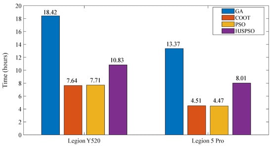
Figure 5.
Comparison between the execution times of the algorithms.
As illustrated in Figure 5, the COOT and PSO algorithms were executed almost simultaneously, completing one run and tuning 12 gains for the conventional PID controllers. In contrast, the GA and HJSPSO algorithms tuned 30 gains for the FOPID controllers, resulting in longer computational times. Specifically, the HJSPSO took 8.01 h on the Legion 5 Pro and 13.37 h on the Legion Y520, while GA took 18.42 h on the Legion Y520 and 13.37 h on the Legion 5 Pro. Despite this, the HJSPSO outperformed GA in terms of computational time and results, making it a promising choice for the investigated application.
Also, we conducted a comparison of the COOT, PSO, and HJSPSO algorithms on the Legion 5 Pro by optimizing only the 12 gains of a conventional PID controller to assess the complexity of the hybrid algorithm in comparison to PSO and COOT. The results are presented in Figure 6. The computational times of the three algorithms are very similar. However, due to the higher complexity of the HJSPSO algorithm, it required more computational time than the PSO and COOT algorithms.
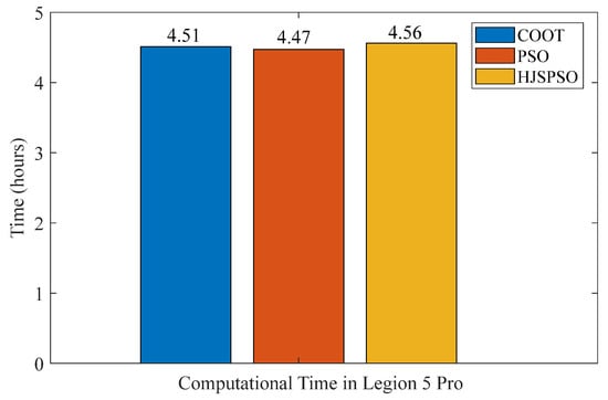
Figure 6.
Comparison between the execution times with 12 gains required to be tuned.
5. Nonlinear Grid-Connected AWS System Steady and Transient Responses
In this part, the results are presented for the AWS grid-connected system that was modeled using MATLAB Simulink with a sampling time of 10 microseconds. To verify the robustness of our proposed controller (HJSPSO-FOPID), the system is first presented during the steady state without any fault condition. Then, the system was subjected at point “F” depicted in Figure 2 to different faults, including unsymmetrical and symmetrical faults.
The Simulink results involve the current position and velocity of the wave energy conversion system with respect to time, the three-phase currents, the stator dq currents, the generated power, the DC link voltage, the grid voltage, the responses of real and reactive powers at the connection point with the grid (point of common coupling (PCC)), and the dq currents at the grid side. Starting with connecting the system and supplying electrical power to the power grid for 100 s, the simulation results during the steady state of normal operation are provided in Figure 7.
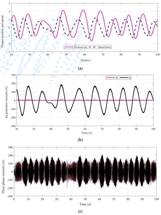
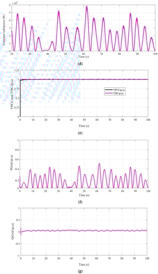
Figure 7.
(a) and of the wave energy conversion device, (b) the quadrature and direct axis currents of the stator, (c) the three-phase generated currents (“” (black), “” (red), and “” (blue)), (d) the real power produced by the linear generator, (e) and , (f) the injected real power (), and (g) the injected reactive power ().
The results show that the dq currents were maintained at the reference values expressed in (36) and (37). This led to the maximization of the generated power similar to [11,20] and the minimization of the stator losses. For the grid-side inverter controllers, both and were maintained at 1 p.u as intended. Also, the power injected was very close to the generated power; in addition, the reactive power fluctuated around zero. This confirms that the controllers achieved the desired goals.
However, as with any type of controller, the steady-state performance is insufficient to test these controllers’ actual performance and reliability. That is why the system was first subjected to a symmetrical 3LG fault after 6.1 s at point F in Figure 2. In this scenario, the breakers successfully cleared the faulty line after 0.1 s of fault occurrence and then successfully reclosed after 0.8 s. The test results are shown in Figure 8.
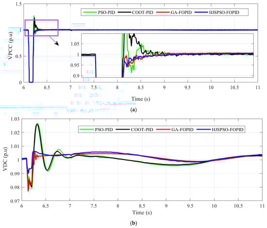
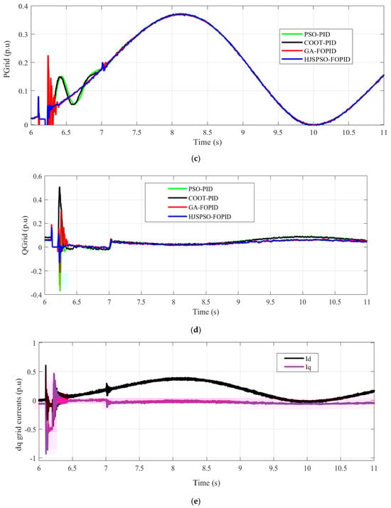
Figure 8.
(a) , (b) , (c) , (d) , and (e) dq grid currents.
A numerical comparison between the performance of these controllers with respect to , , , and is provided in Table 4.
Table 4.
Summary of the performance of the controllers.
The results show that the HJSPSO-FOPID and the GA-FOPID controllers showed ideal performance in preventing from overshooting above 1 p.u compared with the conventional PID controllers. Furthermore, had the lowest overshooting and dip in the case of HJSPSO. The response had the lowest fluctuations and a very quick return to the steady state value of the power in the case of HJSPSO-FOPID. The dq currents at the grid side were also maintained under 1 p.u during the fault conditions. Finally, had the best combination of a reasonable balance between overshooting and undershooting compared with the others. For more validation of the FOPID performance, the unsymmetrical fault responses are shown in Figure 9.
Figure 9.
(a) (1LG), (b) (2LG), and (c) (LL).
The performance of the four controllers during the unsymmetrical faults is summarized in Table 5.
Table 5.
Comparison between the performances of the controllers.
Similar to the symmetrical fault results, the HJSPSO-FOPID controllers outperformed the GA-FOPID, PSO-PID, and COOT-PID controllers and prevented from overshooting above 1 p.u. In summary, without any doubt, the HJSPSO-FOPID had a much better capability in achieving the control goals compared with the GA-FOPID, PSO-PID, and COOT-PID controllers. This made it a more favorable and reliable choice when controlling the grid-connected AWS.
6. Conclusions
This paper presents fractional-order PID controllers for successfully connecting the AWS to the electrical power grid and obtaining the maximum energy harvest from waves. These goals require a back–back converter configuration with six controllers.
In this work, six fractional-order PID controllers were proposed as a replacement for the conventional PID controllers. Each FOPID required five gains to be tuned, leading to a total of thirty gains that needed to be adjusted. That is why the HJSPSO optimization algorithm was employed to obtain the controllers’ gains that minimized the cost function. The performance of this control system was evaluated against the conventional PID controllers that were tuned using the PSO and COOT algorithms and FOPID controllers that were tuned using the GA. The system was subjected to 3LG, 2LG, LG, and LL grid faults during the success of the breakers’ reclosure. The fractional order PID using HJSPSO prevented the grid voltage from overshooting above 1 p.u. The overshooting of in the three-phase to ground fault was roughly ~0.0 p.u in the cases of HJSPSO- and GA-FOPID. However, the overshooting was ~0.28 p.u using the PSO-PID and ~0.23 p.u using the COOT-PID. Additionally, had the lowest overshooting (~0.006 p.u) and dip (0.01 p.u) in the case of HJSPSO compared with an overshooting of ~0.007 p.u in the GA-FOPID and ~0.03 p.u in both PSO- and COOT-PID. Furthermore, the had the lowest fluctuations with a rapid return to the actual generated power in the steady state. The grid dq currents were preserved under 1 p.u during the fault conditions. Finally, had the best combination of a reasonable balance between overshooting (~0.1 p.u) and undershooting (~0.13 p.u) compared with overshooting (~0.23 p.u) and undershooting (~0.37 p.u) in the PSO-PID case, overshooting (~0.5 p.u) and undershooting (~0.02 p.u) in the COOT-PID case, and overshooting (~0.3 p.u) and undershooting (~0.22 p.u) in the GA-FOPID case. The performance was also assessed in the case of unsymmetrical faults. Similarly, the grid voltage had an ideal overshooting of ~0.0 p.u in all unsymmetrical faults. For example, in the LG fault, PSO-PID, COOT-PID, and GA-FOPID had overshooting values of ~0.16 p.u, ~0.25 p.u, and ~0.02 p.u, respectively, compared with the ~0.0 p.u overshooting in the case of HJSPSO-FOPID.
Based on the results, the conclusion was that adopting FOPID controllers provided superior results relative to conventional PID controllers. Consequently, this led to an improvement in the system response during grid instabilities. Future research will focus on implementing more complex and nonlinear controllers suitable for the irregular behavior of waves.
Author Contributions
Conceptualization, A.M.A. and H.M.H.; methodology, S.H.E.A.A. and Z.M.A.; validation, Z.M.A. and A.M.A.; formal analysis, H.M.H.; investigation, S.H.E.A.A.; resources, A.M.A. and H.M.H.; data curation, S.H.E.A.A.; writing—original draft preparation, A.M.A.; writing—review and editing, S.H.E.A.A.; visualization, H.M.H. and S.H.E.A.A.; funding, Z.M.A. All authors read and agreed to the published version of the manuscript.
Funding
The authors extend their appreciation to Prince Sattam bin Abdulaziz University for funding this research work through project number PSAU/2023/01/25317.
Data Availability Statement
Data are contained within the article.
Conflicts of Interest
The authors declare no conflict of interest.
References
- Boyle, G. Renewable Energy: Power for a Sustainable Future, 2nd ed.; Oxford University Press: Oxford, UK, 2004; ISBN 0199261784. [Google Scholar]
- Mahdy, A.; Hasanien, H.M.; Aleem, S.H.E.A.; Al-Dhaifallah, M.; Zobaa, A.F.; Ali, Z.M. State-of-the-Art of the Most Commonly Adopted Wave Energy Conversion Systems. Ain Shams Eng. J. 2023, 15, 102322. [Google Scholar] [CrossRef]
- Archimedes Waveswing—AWS Ocean Energy. Available online: https://awsocean.com/archimedes-waveswing/ (accessed on 29 July 2023).
- Polinder, H.; Mecrow, B.C.; Jack, A.G.; Dickinson, P.; Mueller, M.A. Linear Generators for Direct-Drive Wave Energy Conversion. In Proceedings of the IEEE International Electric Machines and Drives Conference, IEMDC’03, Madison, WI, USA, 1–4 June 2003; Volume 2, pp. 798–804. [Google Scholar]
- De Sousa Prado, M.G.; Gardner, F.; Damen, M.; Polinder, H. Modelling and Test Results of the Archimedes Wave Swing. Proc. Inst. Mech. Eng. Part A J. Power Energy 2006, 220, 855–868. [Google Scholar] [CrossRef]
- Wang, W.; Zhang, H.; Jiang, X.; Yang, X. A High-Order and Efficient Numerical Technique for the Nonlocal Neutron Diffusion Equation Representing Neutron Transport in a Nuclear Reactor. Ann. Nucl. Energy 2024, 195, 110163. [Google Scholar] [CrossRef]
- Zhou, Z.; Zhang, H.; Yang, X. H1-Norm Error Analysis of a Robust ADI Method on Graded Mesh for Three-Dimensional Subdiffusion Problems. Numer. Algorithms 2023, 1–19. [Google Scholar] [CrossRef]
- Yang, X.; Zhang, Q.; Yuan, G.; Sheng, Z. On Positivity Preservation in Nonlinear Finite Volume Method for Multi-Term Fractional Subdiffusion Equation on Polygonal Meshes. Nonlinear Dyn. 2018, 92, 595–612. [Google Scholar] [CrossRef]
- Sá da Costa, J.; Sarmento, A.J.N.; Gardner, F.; Beirão, P.; Brito-Melo, A. Time Domain Model of the AWS Wave Energy Converter. In Proceedings of the 6th European Wave and Tidal Energy Conference, Glasgow, UK, 29 August–2 September 2005; pp. 91–98. [Google Scholar]
- Gieske, P. Model Predictive Control of a Wave Energy Converter: Archimedes Wave Swing. Master’s Thesis, TU Delft, Delft, The Netherlands, 2007; p. 101. [Google Scholar]
- Mahdy, A.; Hasanien, H.M.; Hameed, W.H.A.; Turky, R.A.; Aleem, S.H.E.A.; Ebrahim, E.A. Nonlinear Modeling and Real-Time Simulation of a Grid-Connected AWS Wave Energy Conversion System. IEEE Trans. Sustain. Energy 2022, 13, 1744–1755. [Google Scholar] [CrossRef]
- Wu, F.; Zhang, X.P.; Ju, P.; Sterling, M.J.H. Optimal Control for AWS-Based Wave Energy Conversion System. IEEE Trans. Power Syst. 2009, 24, 1747–1755. [Google Scholar] [CrossRef]
- Hasanien, H.M. Transient Stability Augmentation of a Wave Energy Conversion System Using a Water Cycle Algorithm-Based Multiobjective Optimal Control Strategy. IEEE Trans. Ind. Inform. 2019, 15, 3411–3419. [Google Scholar] [CrossRef]
- Eskandar, H.; Sadollah, A.; Bahreininejad, A.; Hamdi, M. Water Cycle Algorithm—A Novel Metaheuristic Optimization Method for Solving Constrained Engineering Optimization Problems. Comput. Struct. 2012, 110–111, 151–166. [Google Scholar] [CrossRef]
- Mahdy, A.; Hasanien, H.M.; Helmy, W.; Turky, R.A.; Abdel Aleem, S.H.E. Transient Stability Improvement of Wave Energy Conversion Systems Connected to Power Grid Using Anti-Windup-Coot Optimization Strategy. Energy 2022, 245, 123321. [Google Scholar] [CrossRef]
- Naruei, I.; Keynia, F. A New Optimization Method Based on COOT Bird Natural Life Model. Expert Syst. Appl. 2021, 183, 115352. [Google Scholar] [CrossRef]
- Turky, R.A.; Hasanien, H.M.; Alkuhayli, A. Dynamic Stability Improvement of AWS-Based Wave Energy Systems Using a Multiobjective Salp Swarm Algorithm-Based Optimal Control Scheme. IEEE Syst. J. 2022, 16, 79–87. [Google Scholar] [CrossRef]
- Mirjalili, S.; Gandomi, A.H.; Mirjalili, S.Z.; Saremi, S.; Faris, H.; Mirjalili, S.M. Salp Swarm Algorithm: A Bio-Inspired Optimizer for Engineering Design Problems. Adv. Eng. Softw. 2017, 114, 163–191. [Google Scholar] [CrossRef]
- Rasool, S.; Islam, M.R.; Muttaqi, K.M.; Sutanto, D. Coupled Modeling and Advanced Control for Smooth Operation of a Grid-Connected Linear Electric Generator Based Wave-To-Wire System. IEEE Trans. Ind. Appl. 2020, 56, 5575–5584. [Google Scholar] [CrossRef]
- Mahdy, A.; Hasanien, H.M.; Turky, R.A.; Abdel Aleem, S.H.E. Modeling and Optimal Operation of Hybrid Wave Energy and PV System Feeding Supercharging Stations Based on Golden Jackal Optimal Control Strategy. Energy 2023, 263, 125932. [Google Scholar] [CrossRef]
- Chopra, N.; Mohsin Ansari, M. Golden Jackal Optimization: A Novel Nature-Inspired Optimizer for Engineering Applications. Expert Syst. Appl. 2022, 198, 116924. [Google Scholar] [CrossRef]
- Hasanien, H.M. Gravitational Search Algorithm-based Optimal Control of Archimedes Wave Swing-based Wave Energy Conversion System Supplying a DC Microgrid under Uncertain Dynamics. IET Renew. Power Gener. 2017, 11, 763–770. [Google Scholar] [CrossRef]
- Rashedi, E.; Nezamabadi-pour, H.; Saryazdi, S. GSA: A Gravitational Search Algorithm. Inf. Sci. 2009, 179, 2232–2248. [Google Scholar] [CrossRef]
- Sharma, S.; Kapoor, R.; Dhiman, S. A Novel Hybrid Metaheuristic Based on Augmented Grey Wolf Optimizer and Cuckoo Search for Global Optimization. In Proceedings of the 2021 2nd International Conference on Secure Cyber Computing and Communications (ICSCCC), Jalandhar, India, 21–23 May 2021; pp. 376–381. [Google Scholar]
- Adaryani, M.R.; Taher, S.A.; Guerrero, J.M. Model Predictive Control of Direct-Drive Wave Power Generation System Connected to DC Microgrid through DC Cable. Int. Trans. Electr. Energy Syst. 2020, 30, etep12484. [Google Scholar] [CrossRef]
- Valério, D.; Mendes, M.J.G.C.; Beirão, P.; Sá da Costa, J. Identification and Control of the AWS Using Neural Network Models. Appl. Ocean Res. 2008, 30, 178–188. [Google Scholar] [CrossRef]
- Ataşlar-Ayyıldız, B. Robust Trajectory Tracking Control for Serial Robotic Manipulators Using Fractional Order-Based PTID Controller. Fractal Fract. 2023, 7, 250. [Google Scholar] [CrossRef]
- Frikh, M.L.; Soltani, F.; Bensiali, N.; Boutasseta, N.; Fergani, N. Fractional Order PID Controller Design for Wind Turbine Systems Using Analytical and Computational Tuning Approaches. Comput. Electr. Eng. 2021, 95, 107410. [Google Scholar] [CrossRef]
- Yang, B.; Yu, T.; Shu, H.; Zhu, D.; Zeng, F.; Sang, Y.; Jiang, L. Perturbation Observer Based Fractional-Order PID Control of Photovoltaics Inverters for Solar Energy Harvesting via Yin-Yang-Pair Optimization. Energy Convers. Manag. 2018, 171, 170–187. [Google Scholar] [CrossRef]
- Silaa, M.Y.; Barambones, O.; Derbeli, M.; Napole, C.; Bencherif, A. Fractional Order PID Design for a Proton Exchange Membrane Fuel Cell System Using an Extended Grey Wolf Optimizer. Processes 2022, 10, 450. [Google Scholar] [CrossRef]
- Rosas-Jaimes, O.A.; Munoz-Hernandez, G.A.; Mino-Aguilar, G.; Castaneda-Camacho, J.; Gracios-Marin, C.A. Evaluating Fractional PID Control in a Nonlinear MIMO Model of a Hydroelectric Power Station. Complexity 2019, 2019, 9367291. [Google Scholar] [CrossRef]
- Zheng, W.; Luo, Y.; Chen, Y.; Wang, X. A Simplified Fractional Order PID Controller’s Optimal Tuning: A Case Study on a PMSM Speed Servo. Entropy 2021, 23, 130. [Google Scholar] [CrossRef]
- Zamani, M.; Karimi-Ghartemani, M.; Sadati, N.; Parniani, M. Design of a Fractional Order PID Controller for an AVR Using Particle Swarm Optimization. Control Eng. Pract. 2009, 17, 1380–1387. [Google Scholar] [CrossRef]
- Noman, A.M.; Almutairi, S.Z.; Aly, M.; Alqahtani, M.H.; Aljumah, A.S.; Mohamed, E.A. A Marine-Predator-Algorithm-Based Optimum FOPID Controller for Enhancing the Stability and Transient Response of Automatic Voltage Regulators. Fractal Fract. 2023, 7, 690. [Google Scholar] [CrossRef]
- El-Sousy, F.F.M.; Alqahtani, M.H.; Aljumah, A.S.; Aly, M.; Almutairi, S.Z.; Mohamed, E.A. Design Optimization of Improved Fractional-Order Cascaded Frequency Controllers for Electric Vehicles and Electrical Power Grids Utilizing Renewable Energy Sources. Fractal Fract. 2023, 7, 603. [Google Scholar] [CrossRef]
- Daraz, A.; Malik, S.A.; Basit, A.; Aslam, S.; Zhang, G. Modified FOPID Controller for Frequency Regulation of a Hybrid Interconnected System of Conventional and Renewable Energy Sources. Fractal Fract. 2023, 7, 89. [Google Scholar] [CrossRef]
- Nayyef, H.M.; Ibrahim, A.A.; Mohd Zainuri, M.A.A.; Zulkifley, M.A.; Shareef, H. A Novel Hybrid Algorithm Based on Jellyfish Search and Particle Swarm Optimization. Mathematics 2023, 11, 3210. [Google Scholar] [CrossRef]
- Chou, J.-S.; Truong, D.-N. A Novel Metaheuristic Optimizer Inspired by Behavior of Jellyfish in Ocean. Appl. Math. Comput. 2021, 389, 125535. [Google Scholar] [CrossRef]
- Kennedy, J.; Eberhart, R. Particle Swarm Optimization. In Proceedings of the ICNN’95—International Conference on Neural Networks, Perth, Australia, 27 November–1 December 1995; Volume 4, pp. 1942–1948. [Google Scholar]
- Herber, D.R.; Allison, J.T. Wave Energy Extraction Maximization in Irregular Ocean Waves Using Pseudospectral Methods. In Proceedings of the Volume 3A: 39th Design Automation Conference; American Society of Mechanical Engineers, Portland, OR, USA, 4–7 August 2013. [Google Scholar]
- Wu, F.; Ju, P.; Zhang, X.-P.; Qin, C.; Peng, G.J.; Huang, H.; Fang, J. Modeling, Control Strategy, and Power Conditioning for Direct-Drive Wave Energy Conversion to Operate With Power Grid. Proc. IEEE 2013, 101, 925–941. [Google Scholar] [CrossRef]
- Shah, P.; Agashe, S. Review of Fractional PID Controller. Mechatronics 2016, 38, 29–41. [Google Scholar] [CrossRef]
- Podlubny, I. Fractional-Order Systems and PI/Sup/Spl Lambda//D/Sup/Spl Mu//-Controllers. IEEE Trans. Automat. Contr. 1999, 44, 208–214. [Google Scholar] [CrossRef]
- Warrier, P.; Shah, P. Optimal Fractional Pid Controller for Buck Converter Using Cohort Intelligent Algorithm. Appl. Syst. Innov. 2021, 4, 50. [Google Scholar] [CrossRef]
Disclaimer/Publisher’s Note: The statements, opinions and data contained in all publications are solely those of the individual author(s) and contributor(s) and not of MDPI and/or the editor(s). MDPI and/or the editor(s) disclaim responsibility for any injury to people or property resulting from any ideas, methods, instructions or products referred to in the content. |
© 2023 by the authors. Licensee MDPI, Basel, Switzerland. This article is an open access article distributed under the terms and conditions of the Creative Commons Attribution (CC BY) license (https://creativecommons.org/licenses/by/4.0/).