Abstract
In this paper, the Caputo-based fractional derivative optimal control model is looked at to learn more about how the human respiratory syncytial virus (RSV) spreads. Model solution properties such as boundedness and non-negativity are checked and found to be true. The fundamental reproduction number is calculated by using the next-generation matrix’s spectral radius. The fractional optimal control model includes the control functions of vaccination and treatment to illustrate the impact of these interventions on the dynamics of virus transmission. In addition, the order of the derivative in the fractional optimal control problem indicates that encouraging vaccination and treatment early on can slow the spread of RSV. The overall analysis and the simulated behavior of the fractional optimum control model are in good agreement, and this is due in large part to the use of the MATLAB platform.
1. Introduction
Children and the elderly are particularly vulnerable to respiratory illnesses caused by the human respiratory syncytial virus (RSV). Understanding the mechanisms of RSV transmission is crucial for the creation of preventative measures such as vaccinations and antiviral therapies [1,2]. Factors like transmission pathways, population vulnerability, seasonal fluctuations, and viral features all play a role in describing how RSV spreads.
Direct contact with an infected person’s respiratory secretions is the primary mode of transmission for RSV. Droplets can have a role in this. Droplets containing the virus are spread when an infected individual coughs or sneezes, infecting those who come into contact with the droplets [3]. The virus can stay dormant for a while on hard surfaces. Infection can occur after touching a contaminated surface and then touching the face. The airborne particle transmission of RSV is uncommon but possible when an infected person breathes in aerosols.
RSV is one of the most common causes of bronchiolitis and pneumonia in young children, especially infants. Severe RSV infections are more common in the elderly and in people with compromised immune systems. RSV has a clear seasonal pattern, and it is most prevalent in winter. Environmental factors, including temperature and humidity, as well as greater inside congestion due to colder weather, may be to blame for this seasonality; however, this is still only hypothesized. The fact that there are various strains of RSV can have an impact on its transmission kinetics. The virulence and ease of transmission of various strains are unknown. Important determinants of RSV transmission dynamics include the viral load and the length of time an infected person can transmit the virus. The probability of transmission may rise with higher viral loads [4,5]. Despite the fact that multiple candidates are in development, there is currently a lack of licensed vaccinations for RSV. The transmission dynamics of RSV could be drastically altered with the use of a vaccination. Treatment with antiviral drugs has the potential to lessen the severity of RSV infections and, by extension, their ability to spread. One sick person can transfer RSV to many others in what are called "superspreading events". In order to contain RSV outbreaks, it is important to understand the factors that favor their spread [6,7]. The spread of RSV can be slowed if the community as a whole acquires immunity through exposure to the virus or immunization.
Factors like contact rates and viral properties can be incorporated into mathematical models to better understand and predict RSV transmission patterns. The community’s RSV prevalence may be tracked through surveillance systems, allowing for the early detection of epidemics and better planning of public health responses. In order to develop methods to prevent the spread of RSV and lessen its impact on healthcare systems and communities, knowledge of the virus’s transmission dynamics is essential. More study is needed to fully understand the dynamics of RSV transmission and the factors that can be used to limit its spread [8].
Only by delving deeply into optimal control theory and bifurcation analysis can one comprehend the human syncytial respiratory virus (HSRV). Interactions between different parts of the host population and the pathogen, which may have nonlinear properties, add complexity to these processes. In this case, optimal control theory [9] is employed to figure out the most effective ways to lower transmission rates by looking at the state variables and controls that represent different intervention strategies.
Bifurcation analysis is an effective method for elucidating underlying dynamics [10,11,12,13]. When a parameter reaches a critical value, it frequently causes a dramatic change in the system’s behavior, which is studied using this method [14,15]. Possible manifestations of this phenomenon in the context of HSRV include seasonal fluctuations, shifts in social behavior, and the initiation of a vaccine program. In order to foresee important transition points when transmission rates may abruptly increase or decrease, researchers can use bifurcation analysis to detect thresholds in parameters that could lead to novel infection dynamics. Insight into these junctures allows for the development of timely interventions that can forestall an outbreak or improve conditions conducive to virus spread.
Moreover, the concept of bifurcation is also applied in the study of fractional complex valued BAM neural networks by including time delays [16]. Also, bifurcation along with delay is incorporated for control purposes in a chemical reaction model.
Adding optimal control to this framework further emphasizes the flexibility to adjust tactics in response to changing dynamics. The goal is to reduce the number of infections while taking into account the costs of various control measures in order to arrive at the most effective plans for managing the spread of the virus. Additionally, combining data-driven methodologies with mathematical models can make real-time adjustments to control strategies easier to make [17,18,19,20]. Therefore, the interplay between bifurcation analysis and optimal control theory is crucial to not only comprehend the dynamics of HSRV transmission but also develop effective strategies for intervention, which may one day lead to more effective epidemic management and containment [21]. A more methodical and analytical strategy could reduce HSRV’s impact on human societies, making the world a better and safer place for everyone.
Modeling epidemic scenarios with ordinary differential equations (ODEs) greatly benefits from the use of Caputo fractional derivatives as a key mathematical tool [22]. Their inclusion in epidemic models allows for a more nuanced and realistic analysis of the underlying dynamics of infectious diseases. These derivatives are an expansion of traditional derivatives to non-integer order, giving researchers more leeway to account for processes’ innate memory and heritability as they propagate disease. For instance, fractional calculus provides a more realistic representation of the phenomenon of "herd immunity", allowing models to more accurately depict the potential spread of infectious illnesses within a population over time. Furthermore, a fractional stochastic differential equation is used to analyze the propagation of the disease in some existing studies. The stochasticity impacts the outcomes of the model. Moreover, even a slight modification in the parameter value can result in chaotic dynamics, potentially leading to the occurrence of a disease outbreak [23].
The modeling and analysis of disease transmission dynamics are widely applied to observe the impacts induced. In addition, using Caputo fractional derivatives in ODE models of epidemics can be helpful for depicting the more nuanced dynamics of disease transmission and recovery [24,25]. The model can be fine-tuned to more accurately reflect observed data by switching the order of the derivative to represent slower or quicker rates of virus spread. Such adaptability enables a more accurate simulation of transmission-influencing elements such as environmental context, behavioral shifts, and policy interventions, as well as the heterogeneous mixing and connections within the population. Therefore, researchers and policymakers can create more well-informed strategies and make more precise predictions, both of which are essential for coming up with efficient response methods to stem the spread of infectious illnesses [26,27,28,29].
Caputo fractional derivatives can be used in epidemic models to help researchers better understand the complicated and nonlinear dynamics of disease transmission. Human actions, geographic context, and societal and economic conditions all play a role in the spread of infectious diseases. It is possible that common integer-order models can not adequately represent these subtleties. Because of their versatility, fractional derivatives can be used to create models that more accurately reflect real-world conditions, including the spread of infectious diseases and their potential consequences. Thus, by incorporating Caputo fractional derivatives into ODEs, we can create more accurate and nuanced epidemic models, which in turn can lead to better intervention tactics and a better grasp of the complexities of infectious disease dynamics.
The Caputo fractional derivative provides a more nuanced and flexible method of simulating the transmission kinetics of the RSV with ODEs. Fractional derivatives, which account for memory effects and anomalous diffusion, are better suited to modeling the complicated dynamics of RSV transmission, which are often characterized by seasonal outbreaks and a high incidence of reinfections [30]. The Caputo fractional derivative can improve the accuracy and predictive power of ODE models by allowing the incorporation of these memory properties and the capacity to represent various temporal behaviors within a single framework, thereby allowing for a more realistic representation of the disease progression dynamics and providing insights that can guide more targeted and effective intervention strategies in managing and controlling RSV outbreaks [31,32,33].
In the current study, we are motivated by the contributions of the aforementioned scholars; we studied RSV transmission dynamics through fractional optimal control problem and bifurcation analysis for the identification of possible earlier interventions.
The rest of the research study is structured as follows: In Section 2, the formulation of the Caputo model is discussed, while the reasons for using this particular type of fractional operator are explained in Section 3. A detailed qualitative analysis of the Caputo-based model, including the invariant region, non-negativity of the model’s solutions, equilibria, stability, basic reproductive number, and the bifurcationa analysis, is presented in Section 4. The use of optimal control theory for the Caputo model is discussed in Section 5. Several numerical simulations are performed in Section 6, for which the results are discussed in Section 7. The paper concludes and makes future remarks in Section 8.
2. Model Formulation
In this study, we modified the research conducted in [34]; the total population in the study is classified as follows. (i) Susceptible (S): This group consists of population free of virus, but with chance to become infected with possible exposure to the virus in the future. (ii) Exposed (E): This group consists of the virus-exposed population incapable of transmitting the infection. (iii) Infected (I): This group consists of individuals infected with the virus who are infectious. (iv) Recovered (R): This consists of virus-recovered individuals with temporary immunity.
Moreover, the following fundamental assumptions are taken into consideration in the modeling process:
- •
- The total population is assumed to be constant.
- •
- The infection is seasonal.

Table 1.
Description of model variables.

Table 2.
Descriptions of model parameters.
The transmission dynamics of infection is described by the schematic diagram in Figure 1.

Figure 1.
Flow diagram for RSV infection transmission dynamics.
The fractional optimal control model, taking dimensional (fraction of state variables) and conventional form using the same state variables, is
with the following state variable initial conditions: .
3. Why the Caputo Operator? Reasons and Motivation
Fractional calculus is a generalization of conventional integer-order calculus to non-integer orders. For an understanding of the significance and applications of fractional calculus in many branches of science and engineering, see the following recent works, for instance [35,36,37,38,39,40,41,42,43,44]. In mathematical modeling, the Caputo fractional operator is frequently employed as a fractional derivative. The adoption of the Caputo fractional operator in modeling is motivated by a number of factors, and preliminary findings indicate that it can more accurately reflect the behavior of a variety of systems than traditional integer-order models. The justification for employing the Caputo fractional operator in mathematical modeling is thoroughly examined in the following paragraphs.
As a generalization of ordinary differential equations (ODEs), fractional-order differential equations (FODEs) permit orders with non-integer values. One common definition of a fractional derivative is given by Caputo. There are various benefits to using ODE models with Caputo fractional operators to study infectious diseases:
Traits of Memory and Heredity: Memory is an inherent property of fractional derivatives. This suggests that the present status of the system is influenced by factors outside the recent and immediate past in the context of infectious diseases. This is especially important to keep in mind while thinking about diseases, as they might have lasting impacts and long-term dependencies that are not reflected by traditional ODEs. The order of the derivative can be changed from 0 to 1 (or even higher) to model a wide range of dynamics and complexities in disease transmission. The range of behavior between two integer-order models can be represented by a fractional-order model. A more precise fit for empirical data is possible thanks to the continuous transition between distinct models that is possible with FODEs. A derivative of order 1 might describe a straightforward model for the spread of a disease, whereas a derivative of order might capture more complex behaviors. Changing the sequence allows scientists to better fit the model to real-world data. In some cases, models constructed with fractional derivatives have been proven to suit actual data from infectious disease outbreaks better than typical integer-order models. Anomalous diffusion is characterized by non-local motions, long-tail distributions, or superdiffusion, and it can explain why disease transmission occasionally deviates from classical diffusion (e.g., Brownian motion). These processes are well suited to being described by fractional derivatives. Diseases often work on a variety of time scales, from the rapid replication of pathogens to the more gradual development of immune responses, and this complexity must be captured. These multiscale dynamics may be captured more accurately by fractional-order models than by traditional ODEs. Traditional SIR (susceptible–infectious–recovered) models may not be adequate if the age structure of populations evolves towards older ages. Using fractional derivatives to depict the aging process yields a more realistic picture of disease patterns in such populations. Taking into account variation, not everyone in a population will have the same reaction to an infectious agent. One technique to account for this diversity without expanding the model’s number of compartments or parameters is through the use of fractional derivatives. However, it is important to remember that the extra mathematical complexity and computing expense that FODEs incur in exchange for these benefits are equally significant. Furthermore, fractional orders might be difficult to interpret in physical or biological contexts.
In conclusion, the Caputo fractional operator can provide a more nuanced and adaptable framework than standard integer-order ODEs for simulating infectious diseases. But before using it, one should weigh the benefits and drawbacks thoroughly.
4. Analysis of RSV Model
4.1. Invariant Property
Theorem 1.
The solution of the fractional Caputo model (1) is bounded in the invariant region Ω if such that
Proof.
Adding the corresponding terms on the left and right sides of fractional model (1), we obtain
Applying the Laplace transform to the above equation, we obtain
Moreover, based on the literature [45], we obtain the formula
where . In our case, , and taking , we have
Now, Equation (5) becomes
Taking the inverse Laplace transform on both sides of (6), we obtain
where stands for the one-parameter Mittag–Leffler function. In Equation (7), if for any time t, we have the following result:
Therefore, the solution of the fractional model given in (1) is bounded for all time . □
4.2. Non-Negativity Property
Theorem 2.
The solution of fractional model (1) is non-negative in the invariant region.
Proof.
To show the non-negativity of the solution, consider the Caputo model (1) along the axis of each state variable while other state variables vanish on each state variable’s axis, as given below:
where the initial conditions are .
Now, solving each of the preceding fractional derivative, we obtain
The above computations show the non-negativity invariance of the axis.
The solution of model (1) is positive in the plane. Let such that , and . On the considered plane, we have
Using the Caputo fractional mean value theorem, we obtain , . Therefore, using the preceding equation, we obtain , which is a contradiction to our earlier assumptions for . Therefore, any solution is non-negative for all . Similarly, all solution variables are non-negative for all . Therefore, the solution of the constructed model is non-negative.
Hence, based on the Caputo generalized mean value theorem [46], the solution of the infection model (1) is non-negative. □
4.3. Existence and Uniqueness
Theorem 3.
The solution of fractional model (1) exists and is unique.
Proof.
The proof can be shown using fixed-point theory. For the sake of brevity, it is not included but can be found in some existing references such as [28]. □
4.4. Disease-Free Equilibrium
Theorem 4.
The disease-free equilibrium () of the fractional model (1) is given by
The disease-free equilibrium of the fractional model is computed by setting variables representing infected population equal to zero and solving for other variables. Hence, we set in model (1) where the rate of change of state variables vanishes. Thus,
Considering that the control functions are not applied yet, the preceding equations result in
Therefore, we have
Hence, in the extinction of the disease, the model solution tends towards becoming disease-free—the equilibrium point of .
4.5. Endemic Equilibrium State
Theorem 5.
Proof.
The endemic equilibrium of fractional model (1) is computed by solving the subsequent equations to obtain the state variables.
From the third equation, we obtain
Further, we have
At endemic equilibrium, we have
where .
Also, we have
Now, we have
□
4.6. Basic Reproduction Number
The basic reproduction number () is a crucial tool for describing the transmission dynamics of infections in the population. To compute the basic reproduction number, we apply the next-generation matrix method. Now, from fractional model (1), we can obtain the vectors for the new infection and transition terms, respectively, as
The Jacobian matrices F and V obtained from the above vectors, f and v, respectively, at disease-free equilibrium are given by
The next-generation matrix from the above-mentioned matrices F and V is given by
The simplification of the above calculation yields the following:
The eigenvalues of the preceding next-generation matrix are computed as follows:
Since the basic reproduction number is the spectral radius of next-generation matrix, we have the subsequent result:
4.7. Local Stability of the Disease-Free Equilibrium
Theorem 6.
Disease-free equilibrium of fractional model (1) is locally asymptotically stable if .
Proof.
First, we construct Jacobian matrix from fractional model (52)
The two eigenvalues of the preceding matrix are computed as
The signs of the remaining eigenvalues are determined from the determinant and trace of the subsequent matrix, obtained from the reduced matrix J.
Now, trace and let . Moreover, let if .
Therefore, the disease-free equilibrium is locally asymptotically stable if . □
4.8. Bifurcation Analysis
Theorem 7.
Fractional optimal control model (1) exhibits forward bifurcation at critical point .
Proof.
with initial conditions
Let , and be new variables corresponding to , and R such that model (1) transforms to the subsequent equations:
Next, we construct functions as follows:
Let be the bifurcation parameter, obtained from , and let be the RSV-free equilibrium point. Next, the Jacobian matrix J is computed at using new functions. Thus,
The preceding matrix results in two negative eigenvalues:
Next, the subsequent matrix is used to determine the sign of the two eigenvalues:
Similar to the earlier computations, all eigenvalues of J are negative, with one simple eigenvalue. Therefore, is a bifurcation point for fractional model (1). Next, we determine the kind of bifurcation that occurs at . Let the left and right eigenvectors be denoted by V and W, respectively, such that and , with conditions and . Now, from , we have
This implies
Also, gives
This implies
Also, implies
This implies
Next, we compute all second-order partial derivatives of with respect to the new state variables. Moreover, all second-order partial derivatives are zero at except for the following:
Moreover,
Next, we determine coefficients a and b as
Therefore, based on the signs of the bifurcation coefficients, the forward bifurcation occurs at . □
4.9. Stability of Endemic Equilibrium
Theorem 8.
An endemic equilibrium point of the fractional optimal control problem is locally asymptotically stable if and unstable if .
Proof.
In the next section, we have forward bifurcation at . Thus, the theorem is a corollary of the forward bifurcation condition. □
5. Fractional Optimal Control Problem
5.1. Objective Functional
The objective functional J is constructed to minimize the number of infectious and susceptible individuals along with the cost of treatment and vaccination to control the disease. The nature of the cost function is quadratic, and the minimization problem has an objective functional of the following form:
with initial conditions .
The region of admissible control functions is given by
5.2. Hamiltonian Function
The Pontryagin’s maximum principle (PMP) can be applied to solve the fractional optimal control problem [33]. The Hamiltonian function can be constructed from the fractional optimal control problem as
The variables and are adjoint variables corresponding to the state variables , and R, respectively.
5.3. Adjoint System
The system of adjoint variables can be constructed from the Hamiltonian function using the following relations:
Therefore, the adjoint system is
5.4. Optimal Control
Optimal control functions and are computed from the following equations:
Thus, we obtain:
5.5. Optimality System
The optimality system constructed from the adjoint system and fractional optimal control problem is
with conditions , .
6. Numerical Simulation
Numerical simulation depicts the qualitative behavior of the dynamical system. The solution of the fractional optimal control is solved using the MATLAB code described in [33]. Moreover, variables’ initial size and parameters values are given subsequently. , .
7. Results and Discussion
The state of the implemented control functions is shown in Figure 2. Furthermore, the simulations demonstrate that immunization is a more effective strategy to prevent RSV infection than treatment after infection.
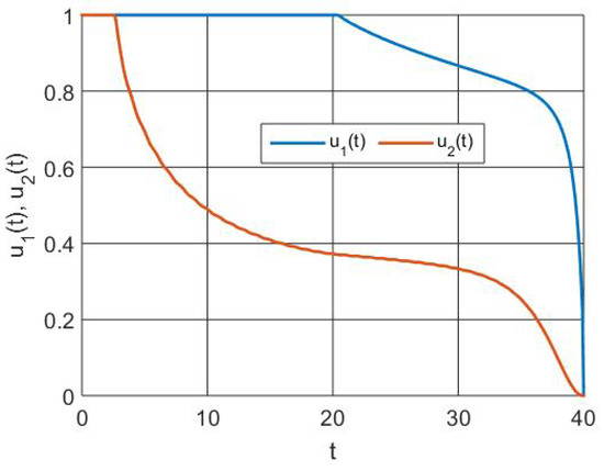
Figure 2.
Simulation of control functions.
The trends in the sensitive population size without and with control actions are shown in Figure 3. Additionally, the figure shows how the availability of an efficient vaccine aids susceptible populations in building immunity and moving on to another class. However, a recent increase in the number of susceptible people is due to lack of vaccination.
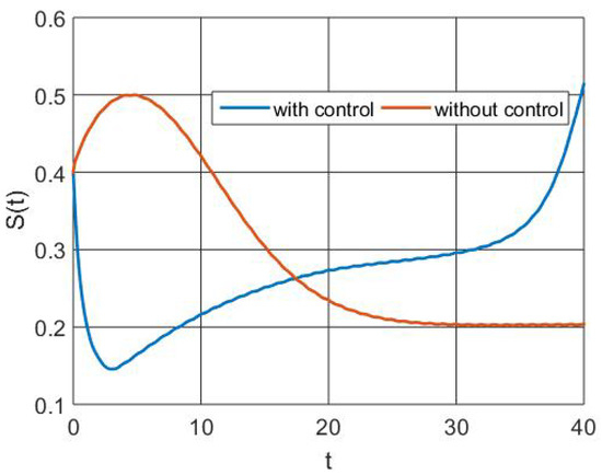
Figure 3.
Simulation of susceptible population dynamics.
The exposed population size is shown in Figure 4 with and without control measures. This demonstrates how intervention with ideal controls lowers the number of people exposed to RSV using the higher-order derivative as a result of immunization and therapy via memory activation.
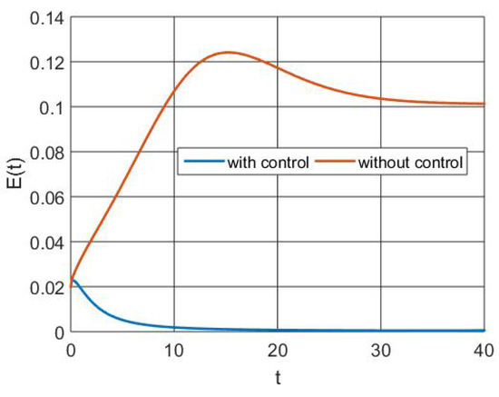
Figure 4.
Simulation of exposed population dynamics.
The infectious population size is shown in Figure 5 with and without control measures. It demonstrates that intervention with the best controls reduces the number of infected people.
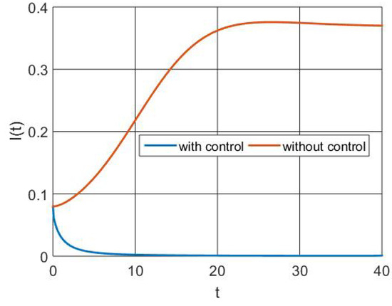
Figure 5.
Simulation of infectious population dynamics.
The regenerated population size is shown in Figure 6 with and without control treatments. It demonstrates that effective optimal controls during intervention enhance the frequency of people recovering from RSV with immunity. However, if a population loses its immunity, it becomes smaller.
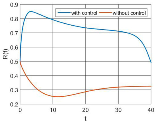
Figure 6.
Simulation of recovered population dynamics.
Figure 7 illustrates the reduction in the susceptible population size caused by intervention through memory effect activation for vaccination uptake.
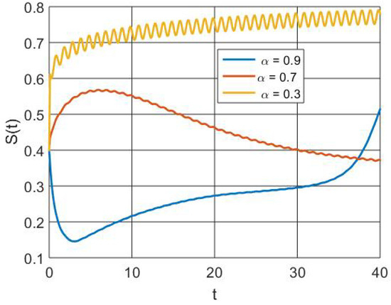
Figure 7.
Simulation of susceptible population dynamics with different orders of derivatives.
Figure 8 illustrates how the exposed population size decreases as a result of treatment and vaccine interventions that activate memory effects.
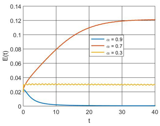
Figure 8.
Simulation of exposed population dynamics with different orders of derivatives.
The infectious population size decrease is depicted in Figure 9 with a higher order of derivative due to interaction with therapy via the activation of the memory effect.
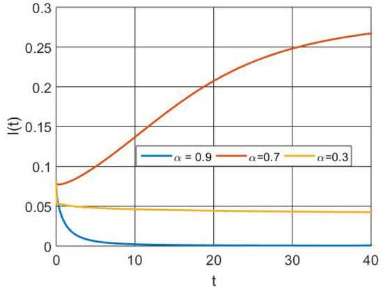
Figure 9.
Simulation of infectious population dynamics with different orders of derivatives.
Figure 10 depicts the increased population size regained as a result of vaccination and therapy that activates the memory effect. Figure 11 depicts the that, at the initial level, the number of susceptible individuals decreases due to infection and vaccination, whereas in the active involvement of control measures (vaccination and treatment), the numbers of RSV-infected individuals decrease. Figure 12 depicts that the basic reproduction number decreases as the recovery rate of individuals increases. Basically, the basic reproduction number and recover rate are inversely proportional. Figure 13 depicts that the basic reproduction number increases as the transmission rate of individuals increases. Basically, the basic reproduction number and recover rate are directly proportional.
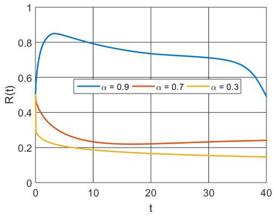
Figure 10.
Simulation of recovered population dynamics with different orders of derivatives.

Figure 11.
Simulation of population dynamics.
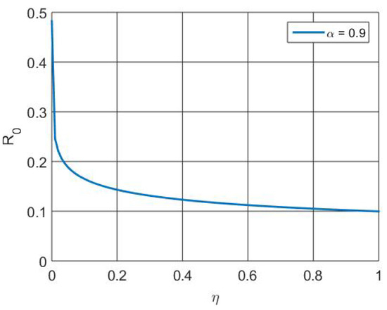
Figure 12.
Simulation of versus parameter .
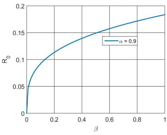
Figure 13.
Simulation of versus parameter .
8. Conclusions
This work examines the fractional optimal control model to explain how optimal control intervention affects the dynamics of RSV virus spread. Additionally, effective control measures such as immunization and treatment lead to the social abolition of RSV infection. This study only demonstrates how acquiring immunity against RSV infection through early vaccination provides effective health performance. The fractional optimal control model’s order of derivative provides information on early vaccination and treatment activation. The higher the derivative order, the more likely people are to receive information and participate in vaccination and treatment. On the other hand, the model shows forward bifurcation when the basic reproduction number reaches unity, and RSV infection extinguishes if the basic reproduction number is smaller than unity, but the illness persists in the population otherwise. Further, this research is expected to be extended to fractional optimal control where the total population is not constant. Also, due to the dual appearance of infections, we recommend that researchers consider the co-infection of RSV with other infections using a fractional optimal control problem.
Author Contributions
M.A.: funding, review and editing. J.A.: funding, review and editing. K.R.C.: conceptualization, formal analysis, writing—review and editing. S.Q.: formal analysis, investigation, software, visualization, writing—original draft. All authors have read and agreed to the published version of the manuscript.
Funding
This work was supported by the Deanship of Scientific Research, Vice Presidency for Graduate Studies and Scientific Research, King Faisal University, Saudi Arabia (grant no. 5469).
This study is supported via funding from Prince Sattam bin Abdulaziz University, project number
(PSAU/2024/R/1445).
Institutional Review Board Statement
Not applicable.
Data Availability Statement
Data sharing is not relevant to this paper, as no data sets were produced or evaluated during the present investigation.
Conflicts of Interest
The authors declare that they have no conflicts of interest.
References
- Lang, J.C. Use of mathematical modelling to assess respiratory syncytial virus epidemiology and interventions: A literature review. J. Math. Biol. 2022, 84, 26. [Google Scholar] [CrossRef]
- Beauchemin, C.A.; Kim, Y.I.; Yu, Q.; Ciaramella, G.; DeVincenzo, J.P. Uncovering critical properties of the human respiratory syncytial virus by combining in vitro assays and in silico analyses. PLoS ONE 2019, 14, e0214708. [Google Scholar] [CrossRef] [PubMed]
- Sungchasit, R.; Tang, I.M.; Pongsumpun, P. Mathematical Modeling: Global Stability Analysis of Super Spreading Transmission of Respiratory Syncytial Virus (RSV) Disease. Computation 2022, 10, 120. [Google Scholar] [CrossRef]
- Hodgson, D. Mathematical Modelling and Cost-Effectiveness of Future RSV Intervention Strategies. Ph.D. Thesis, UCL (University College London), London, UK, 2020. [Google Scholar]
- Mezei, A.; Cohen, J.; Renwick, M.J.; Atwell, J.; Portnoy, A. Mathematical modelling of respiratory syncytial virus (RSV) in low-and middle-income countries: A systematic review. Epidemics 2021, 35, 100444. [Google Scholar] [CrossRef] [PubMed]
- Kombe, I.K.; Agoti, C.N.; Munywoki, P.K.; Baguelin, M.; Nokes, D.J.; Medley, G.F. Integrating epidemiological and genetic data with different sampling intensities into a dynamic model of respiratory syncytial virus transmission. Sci. Rep. 2021, 11, 1463. [Google Scholar] [CrossRef] [PubMed]
- Kaslow, R.A.; Bell, D.M. Epidemiology and Control: From Principles to Pandemics. In Viral Infections of Humans: Epidemiology and Control; Springer: Berlin/Heidelberg, Germany, 2022; pp. 1–80. [Google Scholar]
- Pitzer, V.E.; Viboud, C.; Alonso, W.J.; Wilcox, T.; Metcalf, C.J.; Steiner, C.A.; Haynes, A.K.; Grenfell, B.T. Environmental drivers of the spatiotemporal dynamics of respiratory syncytial virus in the United States. PLoS Pathog. 2015, 11, e1004591. [Google Scholar] [CrossRef]
- Boukhouima, A.; Lotfi, E.M.; Mahrouf, M.; Rosa, S.; Torres, D.F.; Yousfi, N. Stability analysis and optimal control of a fractional HIV-AIDS epidemic model with memory and general incidence rate. Eur. Phys. J. Plus 2021, 136, 1–20. [Google Scholar] [CrossRef]
- Luo, D. Bifurcation Theory and Methods of Dynamical Systems; World Scientific: Singapore, 1997; Volume 15. [Google Scholar]
- Castillo-Chavez, C.; Song, B. Dynamical models of tuberculosis and their applications. Math. Biosci. Eng. 2004, 1, 361–404. [Google Scholar] [CrossRef]
- Huang, C.; Wang, J.; Chen, X.; Cao, J. Bifurcations in a fractional-order BAM neural network with four different delays. Neural Netw. 2021, 141, 344–354. [Google Scholar] [CrossRef]
- Hou, H.S.; Zhang, H. Stability and hopf bifurcation of fractional complex–valued BAM neural networks with multiple time delays. Appl. Math. Comput. 2023, 450, 127986. [Google Scholar] [CrossRef]
- Saha, S.; Samanta, G.; Nieto, J.J. Epidemic model of COVID-19 outbreak by inducing behavioural response in population. Nonlinear Dyn. 2020, 102, 455–487. [Google Scholar] [CrossRef] [PubMed]
- Saha, S.; Samanta, G.; Nieto, J.J. Impact of optimal vaccination and social distancing on COVID-19 pandemic. Math. Comput. Simul. 2022, 200, 285–314. [Google Scholar] [CrossRef] [PubMed]
- Mua, D.; Xub, C.; Liua, Z.; Panga, Y. Further Insight Into Bifurcation and Hybrid Control Tactics of a Chlorine Dioxide–Iodine–Malonic Acid Chemical Reaction Model Incorporating Delays. MATCH Commun. Math. Comput. Chem. 2023, 89, 529–566. [Google Scholar] [CrossRef]
- Giordano, G.; Blanchini, F.; Bruno, R.; Colaneri, P.; Di Filippo, A.; Di Matteo, A.; Colaneri, M. Modelling the COVID-19 epidemic and implementation of population-wide interventions in Italy. Nat. Med. 2020, 26, 855–860. [Google Scholar] [CrossRef] [PubMed]
- Boccaletti, S.; Mindlin, G.; Ditto, W.; Atangana, A. Closing editorial: Forecasting of epidemic spreading: Lessons learned from the current covid-19 pandemic. Chaos Solitons Fractals 2020, 139, 110278. [Google Scholar] [CrossRef]
- Ndaïrou, F.; Area, I.; Nieto, J.J.; Torres, D.F.M. Mathematical modeling of COVID-19 transmission dynamics with a case study of Wuhan. Chaos Solitons Fractals 2020, 135, 109846. [Google Scholar] [CrossRef]
- Lima, L.S. Dynamics based on analysis of public data for spreading of disease. Sci. Rep. 2021, 11, 12177. [Google Scholar] [CrossRef]
- Kar, T.; Nandi, S.K.; Jana, S.; Mandal, M. Stability and bifurcation analysis of an epidemic model with the effect of media. Chaos Solitons Fractals 2019, 120, 188–199. [Google Scholar] [CrossRef]
- Qureshi, S.; Yusuf, A. Fractional derivatives applied to MSEIR problems: Comparative study with real world data. Eur. Phys. J. Plus 2019, 134, 171. [Google Scholar] [CrossRef]
- Lima, L.d.S. Fractional stochastic differential equation approach for spreading of diseases. Entropy 2022, 24, 719. [Google Scholar] [CrossRef]
- Al-Hoceima, E. 1ére Journée sur l’Intelligence Artificielle & Mathématiques Appliquées 04 Mai 2023 ENSA Al-Hoceima. Available online: https://www.researchgate.net/profile/Younes-Abouelhanoune/publication/370659883_JIAMA'23_Book_Abstracts/links/6470cc8d6a3c4c6efbe1f2ce/JIAMA23-Book-Abstracts.pdf (accessed on 17 November 2023).
- Soulaimani, S.; Kaddar, A. Analysis and Optimal Control of a Fractional Order SEIR Epidemic Model with General Incidence and Vaccination. IEEE Access 2023, 11, 81995–82002. [Google Scholar] [CrossRef]
- Padder, A.; Almutairi, L.; Qureshi, S.; Soomro, A.; Afroz, A.; Hincal, E.; Tassaddiq, A. Dynamical Analysis of Generalized Tumor Model with Caputo Fractional-Order Derivative. Fractal Fract. 2023, 7, 258. [Google Scholar] [CrossRef]
- Nisar, K.S.; Farman, M.; Abdel-Aty, M.; Cao, J. A review on epidemic models in sight of fractional calculus. Alex. Eng. J. 2023, 75, 81–113. [Google Scholar] [CrossRef]
- Qureshi, S.; Jan, R. Modeling of measles epidemic with optimized fractional order under Caputo differential operator. Chaos Solitons Fractals 2021, 145, 110766. [Google Scholar] [CrossRef]
- Boukhouima, A.; Hattaf, K.; Lotfi, E.M.; Mahrouf, M.; Torres, D.F.; Yousfi, N. Lyapunov functions for fractional-order systems in biology: Methods and applications. Chaos Solitons Fractals 2020, 140, 110224. [Google Scholar] [CrossRef]
- Sidi Ammi, M.R.; Tahiri, M.; Tilioua, M.; Zeb, A.; Khan, I.; Andualem, M. Global analysis of a time fractional order spatio-temporal SIR model. Sci. Rep. 2022, 12, 5751. [Google Scholar] [CrossRef]
- Ahmad, B.; Nieto, J.J.; Alsaedi, A.; El-Shahed, M. A study of nonlinear Langevin equation involving two fractional orders in different intervals. Nonlinear Anal. Real World Appl. 2012, 13, 599–606. [Google Scholar] [CrossRef]
- Jajarmi, A.; Baleanu, D.; Sajjadi, S.S.; Nieto, J.J. Analysis and some applications of a regularized ψ–Hilfer fractional derivative. J. Comput. Appl. Math. 2022, 415, 114476. [Google Scholar] [CrossRef]
- Rosa, S.; Torres, D.F. Optimal control of a fractional order epidemic model with application to human respiratory syncytial virus infection. Chaos Solitons Fractals 2018, 117, 142–149. [Google Scholar] [CrossRef]
- Rosa, S.; Torres, D.F. Numerical Fractional Optimal Control of Respiratory Syncytial Virus Infection in Octave/MATLAB. Mathematics 2023, 11, 1511. [Google Scholar] [CrossRef]
- Ahmad, H.; Khan, M.; Ahmad, I.; Omri, M.; Alotaibi, M. A meshless method for numerical solutions of linear and nonlinear time-fractional Black–Scholes models. AIMS Math. 2023, 8, 19677–19698. [Google Scholar] [CrossRef]
- Alquran, M.; Sulaiman, T.; Yusuf, A.; Alshomrani, A.; Baleanu, D. Nonautonomous lump-periodic and analytical solutions to the (3+1)-dimensional generalized Kadomtsev–Petviashvili equation. Nonlinear Dyn. 2023, 111, 11429–11436. [Google Scholar] [CrossRef]
- Latif, S.; Sabir, Z.; Raja, M.; Altamirano, G.; Núñez, R.; Gago, D.; Sadat, R.; Ali, M. IoT technology enabled stochastic computing paradigm for numerical simulation of heterogeneous mosquito model. Multimed. Tools Appl. 2023, 82, 18851–18866. [Google Scholar] [CrossRef]
- Qayyum, M.; Ahmad, E.; Tauseef Saeed, S.; Ahmad, H.; Askar, S. Homotopy perturbation method-based soliton solutions of the time-fractional (2+1)-dimensional Wu–Zhang system describing long dispersive gravity water waves in the ocean. Front. Phys. 2023, 11, 1178154. [Google Scholar] [CrossRef]
- Sabir, Z.; Guirao, J. A soft computing scaled conjugate gradient procedure for the fractional order Majnun and Layla romantic story. Mathematics 2023, 11, 835. [Google Scholar] [CrossRef]
- Souayeh, B.; Sabir, Z. Designing Hyperbolic Tangent Sigmoid Function for Solving the Williamson Nanofluid Model. Fractal Fract. 2023, 7, 350. [Google Scholar] [CrossRef]
- Zarin, R.; Khan, M.; Khan, A.; Yusuf, A. Deterministic and fractional analysis of a newly developed dengue epidemic model. Waves Random Complex Media 2023. [Google Scholar] [CrossRef]
- Zil-E-Huma; Butt, A.; Raza, N.; Ahmad, H.; Ozsahin, D.; Tchier, F. Different solitary wave solutions and bilinear form for modified mixed-KDV equation. Optik 2023, 287, 171031. [Google Scholar] [CrossRef]
- Hashemi, M.; Mirzazadeh, M.; Ahmad, H. A reduction technique to solve the (2 + 1)-dimensional KdV equations with time local fractional derivatives. Opt. Quantum Electron. 2023, 55, 721. [Google Scholar] [CrossRef]
- Sulaiman, T.A.; Yusuf, A.; Alshomrani, A.S.; Baleanu, D. Wave solutions to the more general (2 + 1)-dimensional Boussinesq equation arising in ocean engineering. Int. J. Mod. Phys. B 2023, 2350214. [Google Scholar] [CrossRef]
- Podlubny, I. Fractional Differential Equations: An Introduction to Fractional Derivatives, Fractional Differential Equations, to Methods of Their Solution and Some of Their Applications; Academic Press: San Diego, CA, USA, 1998. [Google Scholar]
- Yaro, D.; Apeanti, W.O.; Akuamoah, S.W.; Lu, D. Analysis and optimal control of fractional-order transmission of a respiratory epidemic model. Int. J. Appl. Comput. Math. 2019, 5, 1–21. [Google Scholar] [CrossRef] [PubMed]
Disclaimer/Publisher’s Note: The statements, opinions and data contained in all publications are solely those of the individual author(s) and contributor(s) and not of MDPI and/or the editor(s). MDPI and/or the editor(s) disclaim responsibility for any injury to people or property resulting from any ideas, methods, instructions or products referred to in the content. |
© 2024 by the authors. Licensee MDPI, Basel, Switzerland. This article is an open access article distributed under the terms and conditions of the Creative Commons Attribution (CC BY) license (https://creativecommons.org/licenses/by/4.0/).