Some Fractional Stochastic Models for Neuronal Activity with Different Time-Scales and Correlated Inputs

Abstract

In order to describe neuronal dynamics on different time-scales, we propose a stochastic model based on two coupled fractional stochastic differential equations, with different fractional orders. For the specified choice of involved functions and parameters, we provide three specific models, with/without leakage, with fractional/non-fractional correlated inputs. We give explicit expressions of the process representing the voltage variation in the neuronal membrane. Expectation values and covariances are given and compared. Numerical evaluations of the average behaviors of involved processes are presented and discussed.

1. Introduction

The fractional calculus ([1,2]) used in the framework of stochastic modeling (see [3] and references therein) allows a twofold advantage: a mathematical generalization of existing stochastic processes and the construction of more refined models, including much more detailed phenomenological evidence. Specifically, in neuronal modeling, the introduction of fractional non local operators in stochastic equations allows the description of confluent dynamics on different time scales. This is the idea on which this contribution is written: to provide a fractional stochastic model that generalizes the previous ones, but it is also suitable to describe dynamics such as those involved in the neuronal activity subject to interactions and inputs of different nature.

In the scientific literature of recent decades, we can see a very large number of contributions devoted to refine existing stochastic neuronal models, among them the well-known Leaky Integrate-and-Fire (LIF) model, in order to enrich the description with further phenomenological aspects. The purpose of such refinements is, essentially, that to include adaptation behaviors, correlated inputs, correlation between inputs, evolution on different time-scales, etc. (see, for instance, [4,5,6,7]). The stochastic LIF model, essentially based on a stochastic Langevin equation ([8]), has become unsatisfactory: it only includes a delta-correlated white noise, whereas correlated inputs (see, for instance, [9]), in some cases modeled by colored noises ([10]), appear more satisfactory to explain the high variability in the neuronal response to inputs and adaptation phenomena ([9,11]). Furthermore, its intrinsic Markov property, or equivalently, memory-less property, makes it not suitable to model adaptation dynamics, or any other firing activity affected by memory effects. Moreover, only one time-scale can be considered, even if different time-scales seem to be mandatory when it is required to include the effects of the activity of ionic channels and/or synaptic inputs on the neuronal firing. In some previous contributions (see [12,13,14,15] and references therein), some specialized LIF models were provided in order to satisfy such kind of requirements.

Inspired by papers [10,16], we proposed in [15] a LIF model with a colored noise by using a time-non-homogeneous Gauss–Markov (GM) process. Approximations of the first passage time (FPT), whose probability density is not available in closed form, for such a process through a constant level (the firing threshold) was obtained and discussed with some others such as those in [10,17]. Successively, some further investigations about firing rates were provided, and specifically in [18], a modified LIF-type stochastic model was considered with a non-delta correlated input process in place of the white noise. Mathematical tools and simulation approaches were adopted in [18] to perform an analysis of that LIF-type model with specified correlated inputs. The theory of integrated GM processes ([12] ) was evoked in the study of such kinds of models. Indeed, the neuronal voltage was modeled by means of the integral over time of a correlated input, an Ornstein–Uhlenbeck (OU) process. In [12], advances in the study of fractional integrals applied to GM processes were made in order to devise more general models, also in the context of the neuronal modeling. Finally, with the aim to put together the strategy to include the correlated input ([15,18]) and the use of fractional integrals ([12]), in [14], we proposed a first neuronal model based on the fractional integral of a correlated OU process. The joint effect of these two approaches, separately considered in previous papers, was discussed in [14].

The motivation of the present paper is that to provide a neuronal model improved respect to that presented in [14] and oriented to gain a mathematical generalization. From this improved version new specialized neuronal models can be derived. Here, our specific purpose is to study a system of two coupled fractional stochastic equations by which it is possible to describe the dynamics of the neuronal membrane voltage by means of the solution process subject to an input modeled by another process, possibly evolving on a different time-scale.

Specifically, the neuronal activity is modeled by the process denoted by $V\left(t\right)$ as the $\alpha$-fractional time integral of the input process, denoted by $\eta \left(t\right),$ evolving on a different more or less finer time-scale tuned by a fractional order $\beta .$ The values of the fractional orders $\alpha$ and $\beta$ can be chosen on the basis of neuro-physiological conditions and evidence.

The novelty of the proposed model is in the use of fractional derivatives and integrals in place of the classical ones for modeling both the voltage of the neuronal membrane and a correlated input. Indeed, due to the non-locality property, the use of fractional operators is suggested by the need to model a sort of “memory”in the evolution of the neuronal membrane voltage and in the input itself. Models including memory effects are essentially based on fractional Langevin equations, or Langevin equations with colored noise or correlated inputs ([10,17,18]). Here, in particular, we consider fractional Langevin equations and a correlated input.

The present paper is organized as follows: in Section 2, we define the general model based on two fractional coupled stochastic equations. Modeling justifications and biological interpretation are discussed in Section 2.1. The theoretical assumptions for the existence of solutions are specified in Section 2.2, which is dedicated to the mathematical setting for the general fractional model ([2,19]). Then, in successive sections, we derive specific models for different choices of the involved functions and the fractional orders $\alpha$ and $\beta$. Specifically, we consider three cases: Model 1 (without leakage) in Section 3, Model 2 (with leakage) in Section 4, and finally Model 3, which is the general FNM model, in Section 5. For each case, we give the explicit form of the stochastic process $V\left(t\right)$ solving the proposed equations and the corresponding mean and covariance functions. In Section 6, we provide numerical evaluations of the mean of the process $V\left(t\right)$ for the three considered models. In particular, we show and compare the average behavior of the solution processes subject to different inputs and for different values of fractional orders. Finally, in Section 7, we write some conclusions and indicate possible strategies for future simulations of sample paths of such processes and their FPT, useful to estimate neuronal firing times.

2. The General Fractional Model

Here, we denote by FNM the fractional neuronal model, the new model based on the following coupled stochastic differential Equations (SDEs):

FNM model:

$$\begin{array}{ccc}\hfill {\mathcal{D}}^{\alpha }V\left(t\right)& =& f(t,V\left(t\right),V_L)+\sigma \eta \left(t\right),V\left(0\right)=V_0,\hfill \end{array}$$

(1)

$$\begin{array}{ccc}\hfill {\mathcal{D}}^{\beta }\eta \left(t\right)& =& g(t,\eta \left(t\right),I)+\gamma dW\left(t\right),\eta \left(0\right)={\eta }_0,\hfill \end{array}$$

(2)

for $t>0$, $\alpha ,\beta \in (0,1]$ and $\sigma ,\gamma$ (positive) intensity parameters of the stochastic terms $\eta$ and $dW$, respectively. (In Section 2.1, we provide the meaning of all involved functions and parameters). Here, ${\mathcal{D}}^{\alpha }$ and ${\mathcal{D}}^{\beta }$ denote the fractional Caputo derivative ([1,3]), that, for all $f\in C^1$, is defined as follows:

$${\mathcal{D}}^{\nu }\left(f\right)\left(t\right)=\frac{1}{\Gamma (1-\nu )}{\int }_0^t{(t-s)}^{-\nu }{f}^{\prime }\left(s\right)ds,$$

(3)

with $\nu =\alpha ,\beta \in (0,1]$, respectively.

Some mathematical notes:

The fractional differential Equation (1) can also be considered by assuming the existence of the process $V\left(t\right)$ such that:

$$\begin{array}{ccc}\hfill V\left(t\right)& =& V_0+{\mathcal{I}}^{\alpha }\left(f(t,V\left(t\right),V_L)\right)+\sigma {\mathcal{I}}^{\alpha }\left(\eta \left(t\right)\right),\hfill \end{array}$$

(4)

where, for a f continuous function, ${\mathcal{I}}^{\alpha }\left(f\right)$ is the fractional Riemann–Liouville (RL) integral ([20]) of order $\alpha$ defined as follows

$${\mathcal{I}}^{\alpha }\left(f\right)\left(t\right)=\frac{1}{\Gamma \left(\alpha \right)}{\int }_0^t{(t-s)}^{\alpha -1}f\left(s\right)ds,\forall t\in {\mathbb{R}}^{+},$$

(5)

with the Gamma Euler function ($\Gamma$), i.e., $\Gamma \left(z\right)={\int }_0^{+\infty }{t}^{z-1}{e}^{-t}dt,z>0.$ (Recall that we use with the same meaning the double notation ${\mathcal{I}}^{\alpha }\left(f\right)\left(t\right)={\mathcal{I}}^{\alpha }\left(f\left(t\right)\right),$ even if the first one denotes mainly the integral operator ${\mathcal{I}}^{\alpha }\left(f\right)$).

The above fractional integrals evaluated on stochastic processes have to be intended in $pathwise$ interpretation. And, note that the SDE (1) is well defined due to the fact that the Caputo fractional derivative ${\mathcal{D}}^{\alpha }$ is the right inverse of the $RL$ integral of $\alpha$ order (see [20]), i.e., for $f\left(0\right)=0$,

$${{\mathcal{I}}^{\alpha }\mathcal{D}}^{\alpha }\left(f\right)=f,\forall f\in {\mathcal{C}}^1,$$

justified by considering that ${\mathcal{D}}^{\alpha }\left(f\right)={\mathcal{I}}^{1-\alpha }\left(f^{\prime }\right)$ and by taking into account that (see [3] for details)

$${\mathcal{I}}^{\alpha }{\mathcal{D}}^{\alpha }\left(f\right)={\mathcal{I}}^{\alpha }{\mathcal{I}}^{1-\alpha }\left(f^{\prime }\right)={\mathcal{I}}^1{f}^{\prime }=f.$$

Similarly, we assume the existence of an input process $\eta \left(t\right)$ such that:

$$\begin{array}{ccc}\hfill \eta \left(t\right)& =& {\eta }_0+{\mathcal{I}}^{\beta }\left(g(t,\eta (t),I)\right)+\gamma {\mathcal{I}}^{\beta }\left(dW\left(t\right)\right),\eta \left(0\right)={\eta }_0,\hfill \end{array}$$

(6)

Here, the stochastic process ${\mathcal{I}}^{\beta }\left(dW\left(t\right)\right)$ is defined as the Lévy fractional Brownian motion, i.e., we assume that

$${\mathcal{I}}^{\beta }\left(dW\left(t\right)\right)=\frac{1}{\Gamma \left(\nu \right)}{\int }_0^t{(t-\tau )}^{\beta -1}dW\left(\tau \right)$$

(7)

where W is a standard Brownian motion and the integral has to be interpreted in the Itô sense. We remark that only if $\beta \in \left(\frac{1}{2},1\right)$, for fixed $t>0$, the function ${(t-\tau )}^{\beta -1}$ is in $L^2(0,t)$. Thus, the above process is well-defined and it is a Gaussian process starting from 0 at time 0 with probability 1.

Furthermore, the integral forms (4) and (6) allow to apply Theorem 4 of [21], by which we obtain Gaussian solutions.

Finally, we note that a more general model could have been considered if in place of (1) we put the following SDE

$$\begin{array}{ccc}\hfill {\mathcal{D}}^{\alpha }V\left(t\right)& =& f(t,V\left(t\right),V_L)+\sigma \eta \left(t\right)+\zeta d\mathcal{W}\left(t\right),V\left(0\right)=V_0,\hfill \end{array}$$

(8)

with noise terms involving $\mathcal{W}$ and W independent Brownian motions but, in this paper, we consider the special case of FNM model (1) and (2), i.e., we exclude the noise in the first equation in such a way the dynamics of $V\left(t\right)$ is the fractional integral (not perturbed by any noise) of the correlated input $\eta \left(t\right)$. We postpone the study of the FNM model (8) to a future work.

2.1. Some Biological and Modeling Justifications

The adoption of the two above coupled fractional equations allows to use a $\alpha$-fractional stochastic process $V\left(t\right)$ for modeling the neuronal evolution of the membrane voltage and a $\beta$-fractional stochastic correlated input $\eta \left(t\right)$ integrating a current term $I.$ In this sense, we intend that the model can describe neuronal activities on different time-scales modulated by parameters $\alpha$ and $\beta .$

In order to clarify the notation, and to show how this model born as a generalization of the previous ones, we firstly recall the essentials on the neuronal models under consideration. In particular, we recall that the SDE on which the classical stochastic LIF model is based, which is the following stochastic version of the Langevin equation:

$$dV\left(t\right)=-\frac{g_L}{C_m}[V\left(t\right)-V_L]dt+\frac{\sigma }{C_m}dW,V\left(0\right)=V_0,\forall t>0.$$

(9)

The solution process $V\left(t\right)$ stands for the voltage of the neuronal membrane, whereas

$C_m$ is for the membrane capacitance,

$g_L$ is for the leak conductance,

$V_L$ is a specified “resting” value of potential,

$dW\left(t\right)$ is the white noise (with $W\left(t\right)$ a standard Brownian motion (BM)),

$\sigma$ is the intensity (or amplitude) of the noise.

Such terminology, proper of electrical circuits, is justified by the representation of the neuronal membrane similar a capacitor with capacitance $C_m$ in parallel with a resistor (see, for instance, [6,8]). It is possible to have the so-called leakage, because the charge inside the neuronal cell, in absence of the electrical input current, slowly leak through the neuronal membrane towards to the resting potential value $V_L,$ or value after leakage. The leak conductance $g_L$ is such that $1/g_L$ stands for the leak resistance; moreover, the ratio $\frac{C_m}{g_L}$ denotes the membrane time constant.

The occurrence of a neuronal spike, or equivalently a large depolarization of the voltage when this attains a critical value $V_{th},$ is modeled by the FPT of the process $V\left(t\right)$ through the threshold value $V_{th}$. The firing activity corresponds to the emission of sequences of spikes with different rates, and it is the basis of the information transmission between neurons. This mechanism is triggered by electro-chemical variations due to entrance and/or exit of potassium and sodium ions through ionic channels (gates) of the neuronal membrane, but also due to the injections of external currents or synaptic inputs originated by surrounding neurons. It appears clear that these dynamics occur on different time scales. Finally, the membrane voltage, which acts as an integrator of different inputs, can be modeled by means of the solution of a linear differential equation.

More specifically, Equation (2) is a fractional version of the stochastic LIF model (9). Here, we adopted (2), and its solution process $\eta$, for modeling a correlated input that is fractionally integrated by the process $V\left(t\right),$ solving Equation (1).

We again remark that the use of fractional operators is made to include $memory$ in the resultant model. Moreover, the choice of different fractional orders, for the voltage $V\left(t\right)$ and the input $\eta \left(t\right)$, is made for distinguishing the different time-scales of the above-explained dynamics.

Furthermore, in the present model, the $\eta$ process can be view as a synaptic input coming from other neurons and it depends on an additional current term denoted by $I.$ Indeed, I models a synaptic or an injected current embodied in the correlated input $\eta \left(t\right)$. It is possible to perform different mathematical choices for I: beyond the cases of excitatory or inhibitory currents corresponding to positive or negative I terms, we can choose a constant, a periodical function, and a stochastic process [7,18,22], each one with a proper biological justification. Indeed, the form of I can reflect different physiological circumstances; anyway, here, even if we consider a constant $I,$ the suggested above dynamics corresponds to the activity (modeled by $V\left(t\right)$) of a neuron affected by multiple interactions originated from the activity of neighborhood neurons, of correlated inputs, and from codified currents on different time-scales, all summarized in $\eta \left(t\right)$.

A first step in such modeling direction is made in [14], where the proposed model is essentially constructed on the two SDEs:

$$\begin{array}{ccc}\hfill {\mathcal{D}}^{\alpha }V\left(t\right)& =& F(t,V,V_L,\eta ),V\left(0\right)=V_0,\alpha \in (0,1],\hfill \end{array}$$

(10)

$$\begin{array}{ccc}\hfill d\eta \left(t\right)& =& G(t,\eta ,I)dt+\gamma dW\left(t\right),\eta \left(0\right)={\eta }_0.\hfill \end{array}$$

(11)

There, the stochastic correlated input is modeled by the Gaussian process $\eta \left(t\right)$, and a deterministic input current I is involved in its drift. In [14], the functions F and G was suitably specified. In the case, $F(t,V_L,\eta )$ is independent on $V\left(t\right)$, the solution process $V\left(t\right)$ is essentially the fractional integral of an OU-type process and its FPT was estimated by simulations in order to provide approximations of firing times in [14].

Hence, it is now clear that the FNM model (1) and (2) constitutes the generalization of (10) and (11). Indeed, if in (2) we assume $\beta =1,$ the fractional derivative ${\mathcal{D}}^{\beta }$ reduces to the classical derivative and the input process $\eta \left(t\right)$ belongs to the class of Ornstein–Uhlenbeck-type processes that are properly Gauss–Markov correlated processes. In such a case, $\eta \left(t\right)$ is the same considered in (11).

In this way, the membrane potential $V\left(t\right)$ is the $\alpha$–fractional Caputo integral of the correlated input $\eta \left(t\right)$.

Here, the purpose is to study the fractional models derived as particular cases of the proposed fractional FNM model based on the stochastic pair $\left(V\right(t),\eta (t\left)\right)$, solutions of (4) and (6), respectively. Note that the correlated input process $\eta \left(t\right)$ drives the dynamics of membrane voltage $V\left(t\right)$ in different ways, depending on the choice of involved functions $f,g$. In addition, we also justify the adoption of Equations (1) and (2), or equivalently, the coupled processes (4)–(6), remarking that the fractional order $\alpha$ of the derivative in (1) can allow us to describe dynamics of $V\left(t\right)$ on a time-scale different from that of the input $\eta \left(t\right),$ regulated by $\beta$. We expect that the possibility to estimate from the data the values of $\alpha$ and $\beta$ makes actually applicable the model and adherent to the real phenomenon.

2.2. The Mathematical Setting for Fractional SDEs and Solutions

Mathematical results about the resolution of fractional SDEs are scarce and fragmentary. Some papers, including [23,24], are mainly dedicated to the existence and uniqueness of the solutions.

We found (1) and (2) really appropriate for solving SDEs with the method of variation in the constant formula for Caputo fractional differential equations, as described in [25]. Indeed, the assumption of the standard Lipschitz condition on the coefficient of considered SDEs is satisfied.

Referring essentially to the results of [25], we recall definitions and theorems here adapted to the considered fractional SDEs.

Definition 1

(FDe). Let $T>0$ be a real number and $y\left(t\right)$ be a function of $C^1\left([0,T]\right)$. A no-homogeneous linear fractional differential equation (FDe) on the bounded interval $[0,T]$ is the following

$${\mathcal{D}}^{\alpha }y\left(t\right)=Ay\left(t\right)+B\left(t\right),y\left(0\right)=y_0$$

(12)

with ${\mathcal{D}}^{\alpha }$ Caputo derivative as in (3), $\alpha \in (0,1)$, and $A,B\left(t\right)$ measurable and bounded real-valued functions on $[0,T]$.

Remark 1.

We remark that if $B\left(t\right)$ is a stochastic process with sample paths almost surely (a.s.) Hölder continuous (as those we will consider), a stochastic version of FDe can be defined similarly to Equation (12) in path-wise sense.

Note that (1) of proposed model FNM is a stochastic version of the fractional differential equation as (12) with $f(t,V\left(t\right),V_L)\equiv A$ and $\sigma \eta \left(t\right)=B\left(t\right).$

In the next theorem, we provide the explicit form of the solution of FDe (12).

Theorem 1.

The solution of (12) in $[0,T]$ is:

$$y\left(t\right)=E_{\alpha }\left(t^{\alpha }A\right)y_0+{\int }_0^t{(t-s)}^{\alpha -1}{E}_{\alpha ,\alpha }\left({(t-s)}^{\alpha }A\right)B\left(s\right)ds,$$

(13)

with $E_{\alpha ,\alpha }\left(z\right)={\sum }_{k=0}^{\infty }\frac{z^k}{\Gamma (\alpha k+\alpha )}$ and $E_{\alpha }\left(z\right)=E_{\alpha ,1}\left(z\right)$ Mittag–Leffler functions ([26]).

The proof can be found in [27].

Note that in case of a stochastic version of FDe (12) with $B\left(t\right)$, the stochastic process of a complete filtered probability space $(\Omega ,\mathcal{F},{\left\{{\mathcal{F}}_t\right\}}_{t\in [0,\infty )},\mathbb{P})$ with a.s. Hölder continuous paths, the explicit solution given in (18) is the corresponding stochastic process solution.

The definition of a Caputo-fractional SDE follows.

Definition 2

(fractional SDE). Let $T>0$ a real number and the bounded interval $[0,T].$ A fractional stochastic differential equation (fractional SDE) is the following equation:

$${\mathcal{D}}^{\alpha }Y\left(t\right)=AY\left(t\right)+B(t,Y\left(t\right))+\sigma (t,Y\left(t\right))dW\left(t\right)Y\left(0\right)=y_0$$

(14)

with ${\left\{W_t\right\}}_{t\in [0,\infty )}$ a real standard Brownian motion in $(\Omega ,\mathcal{F},{\left\{{\mathcal{F}}_t\right\}}_{t\in [0,\infty )},\mathbb{P})$ a complete filtered probability space, $\alpha \in (1/2,1)$, $A,B,\sigma$ real-valued measurable functions on $[0,T]$ satisfying the following assumptions:

(i)

There exists $L>0$ such that $\forall x,z\in \mathbb{R},\forall t\in [0,T]$

$$\parallel B(t,x)-B(t,z)\parallel +\parallel \sigma (t,x)-\sigma (t,z)\parallel \le L\parallel x-z\parallel$$

(ii)

${\int }_0^T{\parallel B(s,0)\parallel }^{2}ds<\infty ,$ ess${sup}_{s\in [0,T]}\parallel \sigma (s,0)\parallel <\infty .$

Denote by ${\mathbb{L}}^2(\Omega ,{\mathcal{F}}_t,\mathbb{P})$, for any $t\in [0,\infty ),$ the space of mean square integrable functions $f:\Omega \to \mathbb{R}$ with the mean square norm ${\parallel f\parallel }_{ms}=\sqrt{\mathbb{E}(\parallel f{\parallel }^2)}.$ We say that a process $X:[0,\infty )\to {\mathbb{L}}^2(\Omega ,\mathcal{F},\mathbb{P})$ is $\mathbb{F}$-adapted if $X\left(t\right)\in {\mathbb{L}}^2(\Omega ,{\mathcal{F}}_t,\mathbb{P}),\forall t\ge 0.$ Similarly to [23,24], we give the definition of a classical solution of a Caputo fractional SDE as (14).

Definition 3.

A $\mathbb{F}$-adapted process X is solution of (14) with initial condition $X\left(0\right)=X_0\in L^2(\Omega ,{\mathcal{F}}_0,\mathbb{P})$ if it is such that for $t\in [0,T]$:

$$X\left(t\right)=X_0+\frac{1}{\Gamma \left(\alpha \right)}{\int }_0^t{(t-s)}^{\alpha -1}\left(AX\left(s\right)+B(s,X(s\left)\right)\right)ds+\frac{1}{\Gamma \left(\alpha \right)}{\int }_0^t{(t-s)}^{\alpha -1}\sigma (s,X\left(s\right))d{W}_s$$

(15)

or, equivalently,

$$X\left(t\right)=X_0+{\mathcal{I}}^{\alpha }\left(AX\left(t\right)+B(t,X(t\left)\right)\right)+{\mathfrak{I}}^{\alpha }\left(\sigma (t,X\left(t\right))d{W}_t\right).$$

(16)

where ${\mathcal{I}}^{\alpha }$ is the Riemann–Liouville fractional integral as defined in (42) and ${\mathfrak{I}}^{\alpha }\left(\sigma (s,X\left(s\right))d{W}_s\right)$, as in (7), is a stochastic fractional integral defined as

$${\mathfrak{I}}^{\alpha }\left(\sigma (t,X\left(t\right))d{W}_t\right)=\frac{1}{\Gamma \left(\alpha \right)}{\int }_0^t{(t-s)}^{\alpha -1}\sigma (s,X\left(s\right))d{W}_s$$

(17)

that is a generalization of (7).

In [24], it was proved that for any given $X_0$, there exists a unique solution, whose explicit form was found with a variation constant formula. We recall such solution in the next theorem.

Theorem 2.

The solution process of the fractional SDE (14) with initial condition $X\left(0\right)=X_0\in L^2(\Omega ,{\mathcal{F}}_0,\mathbb{P})$, $\forall t\in [0,T],$ is:

$$\begin{array}{ccc}\hfill X\left(t\right)=E_{\alpha }\left(t^{\alpha }A\right)X_0& +& {\int }_0^t{(t-s)}^{\alpha -1}{E}_{\alpha ,\alpha }\left({(t-s)}^{\alpha }A\right)B(s,X_0)ds\hfill \\ & +& {\int }_0^t{(t-s)}^{\alpha -1}{E}_{\alpha ,\alpha }\left({(t-s)}^{\alpha }A\right)\sigma (s,X_0)d{W}_s.\hfill \end{array}$$

(18)

The proof can be found in [25].

Really useful for our application purposes is also the following corollary.

Corollary 1.

Consider the fraction SDE:

$${\mathcal{D}}^{\alpha }X\left(t\right)=AX\left(t\right)+B\left(t\right)+\sigma \left(t\right)dW\left(t\right)X\left(0\right)=X_0$$

(19)

with $B\in {\mathbb{L}}^2([0,T],\mathbb{R})$, $\sigma \in {\mathbb{L}}^{\infty }([0,T],\mathbb{R})$. The explicit expression of the solution of (19) is:

$$\begin{array}{ccc}\hfill X\left(t\right)=E_{\alpha }\left(t^{\alpha }A\right)X_0& +& {\int }_0^t{(t-s)}^{\alpha -1}{E}_{\alpha ,\alpha }\left({(t-s)}^{\alpha }A\right)B\left(s\right)ds\hfill \\ & +& {\int }_0^t{(t-s)}^{\alpha -1}{E}_{\alpha ,\alpha }\left({(t-s)}^{\alpha }A\right)\sigma \left(s\right)d{W}_s.\hfill \end{array}$$

(20)

Note that the case $\alpha =1$ can also be covered by previous theoretical results, taking into account that in such a case the fractional derivative and integral reduce to the corresponding classical ones. Consequently, it is easy to prove that the above results become exactly equal to those well-known in the ordinary and stochastic differential calculus.

Remark 2.

Under all above assumptions we choose the coefficients of fractional SDE here considered, in such a way solutions exist, are unique, and their explicit expressions are also available. The validity of above mathematical results in a compact set $[0,T]$ is perfectly adequate for such kind of models, because the dynamics have to be described until the finite time instant T corresponding to the firing time of the neuron, object of future investigations.

Moreover, about the equations on which the FNM model relies, we remark that (1) is a stochastic version of a FDe as (12) with stochastic term $B\left(t\right)\equiv \eta \left(t\right),$ whereas (2) is a typical fractional SDE as defined in (14).

In next sections, by specifying the involved functions, we identify the coefficients of equations and we provide the explicit expressions of the corresponding solutions.

3. Model 1: The FNM Model without Leakage with a Correlated Input: $\mathit{\alpha }\in (\mathbf{0},\mathbf{1}),\mathit{\beta }=\mathbf{1}$

Beyond the choice of fractional orders, we have to choose the functions f and g involved in the FNM model (1) and (2). The case of

$$f(t,V,V_L)=\frac{g_L}{C_m}{V}_L,g(t,\eta ,I)=-\frac{\eta \left(t\right)-I}{\tau }$$

was extensively studied in [14] as an integrate and fire (IF) neuronal model without leakage.

Here, specifically, we consider that model as a particular case of FNM model (1) and (2) with $\alpha \in (0,1),\beta =1$, essentially based on the two following equations:

$$\begin{array}{ccc}\hfill {\mathcal{D}}^{\alpha }{V}_1\left(t\right)& =& \frac{g_L}{C_m}{V}_L+\sigma \eta \left(t\right),V_1\left(0\right)=V_{1,0},\sigma =1/C_m\hfill \end{array}$$

(21)

$$\begin{array}{ccc}\hfill d\eta \left(t\right)& =& -\frac{\eta \left(t\right)-I}{\tau }dt+\gamma dW\left(t\right),\eta \left(0\right)={\eta }_0,\gamma =\varsigma /\tau .\hfill \end{array}$$

(22)

There, the meaning of the involved parameters $g_L,C_m,V_L$ is the same previously specified in Section 2.1, whereas the addition parameter $\tau$ is related to a characteristic time involved in the correlation time of the input process $\eta \left(t\right),$ (see [15] for details).

In this first instance, we note that Equation (21) includes the input process $\eta \left(t\right)$ in place of a typically noise term.

In particular, for the specified involved functions, we note that Equation (21) is a stochastic version of a FDe as (12) with $A=0,B\left(t\right)=\frac{g_L{V}_L}{C_m}+\sigma \eta \left(t\right),$ whereas (22) is a typical a typical SDE, that can be viewed as the fraction one defined in (19) for $\alpha =1$ and with $A\equiv -\frac{1}{\tau },B\left(t\right)\equiv \frac{I}{\tau },\sigma \left(t\right)\equiv \gamma .$

The input process $\eta \left(t\right)$

We firstly specify that $\eta \left(t\right),$ form the well-known SDE (22), is a non-stationary Gauss–Markov (GM) Ornstein–Uhlenbeck (OU) process. Its mean function is:

$$m\left(t\right)=I+e^{-t/\tau }({\eta }_0-I)$$

(23)

and covariance

$$c(s,t)=\frac{{\varsigma }^2}{2\tau }\left(e^{-(t-s)/\tau }-e^{-(s+t)/\tau }\right),0\le s\le t.$$

(24)

Furthermore, it can be written in terms of a standard BM process $W\left(t\right)$ with the transformed time $r\left(t\right)$, as follows:

$$\eta \left(t\right)=m\left(t\right)+h\left(t\right)W\left(r\right(t\left)\right)$$

(25)

where $r\left(t\right)=\frac{k\left(t\right)}{h\left(t\right)}$ is the increasing function, and functions $k\left(s\right),h\left(t\right)$ are such that the covariance (24) can be factorized as $c(s,t)=k\left(s\right)h\left(t\right)$. Hence, from (24), we have

$$k\left(t\right)=\frac{\varsigma }{2}\left(e^{t/\tau }-e^{-t/\tau }\right),h\left(t\right)=\frac{\varsigma }{\tau }{e}^{-t/\tau }.$$

(26)

Finally, an explicit form of $\eta \left(t\right)$ ([12,14]) is:

$$\eta \left(t\right)=I+e^{-t/\tau }({\eta }_0-I)+\frac{\varsigma }{\tau }{e}^{-t/\tau }W\left(\frac{1}{\tau }(e^{2t/\tau }-1)\right)$$

(27)

from which it is possible to understand how the stochastic input process $\eta \left(t\right)$ depends, in particular, on its initial value ${\eta }_{1,0}$ and on the constant input current term $I$.

The voltage process $V_1\left(t\right)$

From (21) and the last form of process $\eta \left(t\right)$ we can also specify the form of the process $V_1\left(t\right).$ Indeed, first we re-write (21) by using (27), with $V_{1,0}=0,$

$${\mathcal{D}}^{\alpha }{V}_1\left(t\right)=\frac{g_L}{C_m}{V}_L+\sigma \left[I+e^{-t/\tau }({\eta }_0-I)+\frac{\varsigma }{\tau }{e}^{-t/\tau }W\left(\frac{1}{\tau }(e^{2t/\tau }-1)\right)\right]$$

(28)

or, equivalently,

$$V_1\left(t\right)={\mathcal{I}}^{\alpha }\left\{\frac{g_L}{C_m}{V}_L+\sigma \left[I+e^{-t/\tau }({\eta }_0-I)+\frac{\varsigma }{\tau }{e}^{-t/\tau }W\left(\frac{1}{\tau }(e^{2t/\tau }-1)\right)\right]\right\},$$

(29)

and finally, by applying Theorem 1 to Equation (21), we can explicitly write:

$$\begin{array}{cc}{V}_1\left(t\right)\hfill & =\frac{t^{\alpha }}{\Gamma (\alpha +1)}\left(\frac{g_L{V}_L}{C_m}+\sigma I\right)\hfill \\ \hfill & +\sigma ({\eta }_0-I)t^{\alpha }{E}_{1,1+\alpha }(-t/\tau )+\frac{\sigma \varsigma }{\tau }{\mathcal{I}}^{\alpha }\left(e^{-t/\tau }W\left(\frac{1}{\tau }(e^{2t/\tau }-1)\right)\right).\hfill \end{array}$$

(30)

Furthermore, in this, case the process $V_1\left(t\right)$ is Gaussian (see, for instance, [21]) with mean

$$\mathbb{E}\left[V_1\left(t\right)\right]=\frac{t^{\alpha }}{\Gamma (\alpha +1)}\left(\frac{g_L{V}_L}{C_m}+\sigma I\right)+\sigma ({\eta }_0-I)t^{\alpha }{E}_{1,1+\alpha }(-t/\tau )$$

(31)

where $E_{\alpha ,\beta }\left(z\right)={\sum }_{k=0}^{\infty }\frac{z^k}{\Gamma (\alpha k+\beta )}$ is the Mittag–Leffler function ([26]). Its covariance can be derived by considering that the last term in RHS of (30) is the fractional integral of an OU process and from [12], we can specify its covariance as follows:

$$Cov[V_1\left(u\right),V_1\left(t\right)]=\frac{{\sigma }^2{\varsigma }^2}{{\tau }^2}\mathbb{E}\left[{\mathcal{I}}^{\alpha }\left(e^{-u/\tau }W\left(\frac{1}{\tau }(e^{2u/\tau }-1)\right)\right)·{\mathcal{I}}^{\alpha }\left(e^{-t/\tau }W\left(\frac{1}{\tau }(e^{2t/\tau }-1)\right)\right)\right].$$

(32)

In [12] it was proven that

$$\mathbb{E}\left[{\mathcal{I}}^{\alpha }\left(e^{-u/\tau }W\left(\frac{1}{\tau }(e^{2u/\tau }-1)\right)\right)·{\mathcal{I}}^{\alpha }\left(e^{-t/\tau }W\left(\frac{1}{\tau }(e^{2t/\tau }-1)\right)\right)\right]=\frac{1}{{\Gamma }^2\left(\alpha \right)}\left[{\tilde{I}}_1+{\tilde{I}}_2+{\tilde{I}}_3\right]$$

with

$$\begin{array}{ccc}\hfill {\tilde{I}}_1& =& \frac{{\sigma }^2}{\tau }{\int }_0^{u}ds{(u-s)}^{\alpha -1}{e}^{-s/\tau }{\int }_0^{s}dv{(t-v)}^{\alpha -1}sinh(v/\tau ),\hfill \\ \hfill {\tilde{I}}_2& =& \frac{{\sigma }^2}{\tau }{\int }_0^{u}ds{(u-s)}^{\alpha -1}sinh(s/\tau ){\int }_s^{u}dv{(t-v)}^{\alpha -1}{e}^{-v/\tau },\hfill \\ \hfill {\tilde{I}}_3& =& \frac{{\sigma }^2}{\tau }\left({\int }_0^{u}ds{(u-s)}^{\alpha -1}sinh(s/\tau )\right)\left({\int }_u^{t}dv{(t-v)}^{\alpha -1}{e}^{-v/\tau }\right).\hfill \end{array}$$

(33)

Remark 3.

We note that the process $V_1$ preserves also in its covariance the effect of the input $\eta \left(t\right)$ under the fractional integration. This appears evident by writing (32) equivalently as

$$Cov[V_1\left(u\right),V_1\left(t\right)]=\frac{{\sigma }^2{\varsigma }^2}{{\tau }^2}\mathbb{E}\left[{\mathcal{I}}^{\alpha }\left(\eta \left(u\right)\right)·{\mathcal{I}}^{\alpha }\left(\eta \left(t\right)\right)\right].$$

(34)

The analysis carried out constitutes the proof of the following proposition.

Proposition 1.

The voltage process $V_1\left(t\right)$ solution of (21) with the correlated input process $\eta \left(t\right)$ solution of (22) is a Gaussian process with mean (31) and covariance (32).

In [12], a simulation strategy, also applied in [14], for such a process and its FPT can be found.

4. Model 2: The FNM Model with Leakage and a Correlated Input: $\mathit{\alpha }\in (\mathbf{0},\mathbf{1}),\mathit{\beta }=\mathbf{1}$

As suggested in [14], if in the model (10) and (11), that corresponds to FNM model (1) and (2) for $\alpha \in (0,1)$ and $\beta =1$, we set $f(t,V,V_L)=-\frac{g_L}{C_m}[V\left(t\right)-V_L]$ (by inserting the so-called leakage, as in a LIF model), and we have to address the following systems of equations:

$$\begin{array}{ccc}\hfill {\mathcal{D}}^{\alpha }{V}_2\left(t\right)& =& -\frac{g_L}{C_m}[V_2\left(t\right)-V_L]+\frac{\eta \left(t\right)}{C_m},V_2\left(0\right)=V_{2,0}\hfill \end{array}$$

(35)

$$\begin{array}{ccc}\hfill d\eta \left(t\right)& =& -\frac{\eta \left(t\right)-I}{\tau }dt+\frac{\sigma }{\tau }dW\left(t\right),\eta \left(0\right)={\eta }_0.\hfill \end{array}$$

(36)

In particular, for the specified involved functions, we note that Equation (35) is a stochastic version of a FDe as (12) with $A=-\frac{g_L}{C_m},B\left(t\right)=\frac{g_L{V}_L}{C_m}+\frac{\eta \left(t\right)}{C_m},$ whereas (36) is a typical SDE, that can be viewed as the fraction one defined in (19) for $\alpha =1$ and with $A\equiv -\frac{1}{\tau },B\left(t\right)\equiv \frac{I}{\tau },\sigma \left(t\right)\equiv \sigma /\tau .$

Furthermore, note that in order to gain the integral representations of (35) and (36) as in (4) and (6), we also have to set $V_{2,0}=0$.

Remark 4.

More generally, the agreement between a biological circumstance and the choice of initial values $V\left(0\right),\eta \left(0\right)$ can be found when it is required to model the firing activity of neurons with or without reset of the neuronal voltage and of the input after each firing time. This phenomenon is typically called the case of endogenous/exogenous setting: specifically, the endogenous setting is related to the reset of voltage and of the input after a spike (a firing time), otherwise the exogenous case is considered.

Hence, the integral form of equations in (35) and (36) is:

$$V_2\left(t\right)={\mathcal{I}}^{\alpha }\left(-\frac{g_L}{C_m}[V_2\left(t\right)-V_L]\right)\left(t\right)+\frac{1}{C_m}{\mathcal{I}}^{\alpha }(\eta \left)\right(t),V_2\left(0\right)=V_{2,0}=0$$

(37)

and

$$\begin{array}{ccc}\hfill \eta \left(t\right)& =& \mathcal{I}\left(\frac{\eta \left(t\right)-I}{\tau }\right)\left(t\right)+\frac{\sigma }{\tau }\mathcal{I}\left(dW\right)\left(t\right),\eta \left(0\right)={\eta }_0,\hfill \end{array}$$

(38)

where $\mathcal{I}$ is the Lebesgue measure integral and $\mathcal{I}\left(dW\right)\left(t\right)\equiv W\left(t\right),$ in such a way we recognize $\eta \left(t\right)$, the solution of the SDE (38), to be an OU process, essentially the same of the previous section, i.e., a Gauss–Markov OU-type process with mean (23) and covariance (24).

The voltage process $V_2\left(t\right)$

Referring to [1,14,26,28], and by applying Theorem 1 to Equation (35), the process $V_2\left(t\right)$ has the following expression:

$$\begin{array}{cc}{V}_2\left(t\right)\hfill & =V_{2,0}{t}^{\alpha -1}{E}_{\alpha ,\alpha }\left(-\frac{g_L{t}^{\alpha }}{C_m}\right)\hfill \\ \hfill & +{\int }_0^t\left[\frac{g_L{V}_L}{C_m}+\frac{\eta \left(s\right)}{C_m}\right]{(t-s)}^{\alpha -1}{E}_{\alpha ,\alpha }\left(-\frac{g_L{(t-s)}^{\alpha }}{C_m}\right)ds.\hfill \end{array}$$

(39)

Equivalently, by recognizing from (42) that

$${\int }_0^t{(t-s)}^{\alpha -1}{E}_{\alpha ,\alpha }\left(-\frac{g_L{(t-s)}^{\alpha }}{C_m}\right)ds=\Gamma \left(\alpha \right){\mathcal{I}}^{\alpha }\left(E_{\alpha ,\alpha }\left(-\frac{g_L{(t-·)}^{\alpha }}{C_m}\right)\right)\left(t\right)$$

and

$${\int }_0^t\eta \left(s\right){(t-s)}^{\alpha -1}{E}_{\alpha ,\alpha }\left(-\frac{g_L{(t-s)}^{\alpha }}{C_m}\right)ds=\Gamma \left(\alpha \right){\mathcal{I}}^{\alpha }\left(\eta (·)E_{\alpha ,\alpha }\left(-\frac{g_L{(t-·)}^{\alpha }}{C_m}\right)\right)\left(t\right),$$

we can also write:

$$\begin{array}{cc}{V}_2\left(t\right)=V_{2,0}{t}^{\alpha -1}{E}_{\alpha ,\alpha }\left(-\frac{g_L{t}^{\alpha }}{C_m}\right)\hfill & +\frac{g_L{V}_L\Gamma \left(\alpha \right)}{C_m}{\mathcal{I}}^{\alpha }\left(E_{\alpha ,\alpha }\left(-\frac{g_L{(t-·)}^{\alpha }}{C_m}\right)\right)\left(t\right)\hfill \\ \hfill & +\frac{\Gamma \left(\alpha \right)}{C_m}{\mathcal{I}}^{\alpha }\left(\eta (·)E_{\alpha ,\alpha }\left(-\frac{g_L{(t-·)}^{\alpha }}{C_m}\right)\right)\left(t\right).\hfill \end{array}$$

(40)

Hence, $V_2\left(t\right)$ is Gaussian process (see, Theorem 4 in [21]) that, for $V_{2,0}=0$, has the following mean

$$\begin{array}{ccc}\hfill \mathbb{E}\left[V_2\left(t\right)\right]& =& \frac{g_L{V}_L}{C_m}{\int }_0^t{(t-s)}^{\alpha -1}{E}_{\alpha ,\alpha }\left(-\frac{g_L{(t-s)}^{\alpha }}{C_m}\right)ds\hfill \\ & +& \frac{1}{C_m}{\int }_0^{t}m\left(s\right){(t-s)}^{\alpha -1}{E}_{\alpha ,\alpha }\left(-\frac{g_L{(t-s)}^{\alpha }}{C_m}\right)ds\hfill \end{array}$$

(41)

where $m\left(t\right)$ is the mean of $\eta \left(t\right)$ as specified in (23).

Equation (40) shows that the $V_2\left(t\right)$ process involves fractional integrals of a Mittag–Leffler function and of the process $\eta \left(t\right)$. In particular, recalling the explicit expression of $\eta \left(t\right)$ in (27), and setting $V_{2,0}=0$ in (40), we have that the stochastic term of $V_2\left(t\right)$ can be specifically written as

$${\mathcal{I}}^{\alpha }\left(\eta (·)E_{\alpha ,\alpha }\left(-\frac{g_L{(t-·)}^{\alpha }}{C_m}\right)\right)\left(t\right)$$

(42)

$$={\int }_0^t{(t-s)}^{\alpha -1}{E}_{\alpha ,\alpha }\left(-\frac{g_L{(t-s)}^{\alpha }}{C_m}\right)\left[I+e^{-s/\tau }({\eta }_0-I)+\frac{\varsigma }{\tau }{e}^{-s/\tau }W\left(\frac{1}{\tau }(e^{2s/\tau }-1)\right)\right]ds.$$

(43)

From (43), we distinguish the stochastic terms that contributes to the calculus of the covariance. Indeed, recalling $r\left(t\right)=\frac{1}{\tau }(e^{2t/\tau }-1)$ and setting $W_r\left(t\right)=W\left(\frac{1}{\tau }(e^{2t/\tau }-1)\right)$ and

$${\mathcal{J}}^{\left(E_{\alpha }\right)}\left(W_r\right)\left(t\right)={\int }_0^t{(t-s)}^{\alpha -1}{E}_{\alpha ,\alpha }\left(-\frac{g_L{(t-s)}^{\alpha }}{C_m}\right)e^{-s/\tau }{W}_r\left(s\right)ds,$$

(44)

the covariance of $V_2\left(t\right)$ can be finally written (in terms of the Brownian motion) as

$$Cov[V_2\left(u\right),V_2\left(t\right)]=\frac{{\sigma }^2}{{\tau }^2{C}_m^2}cov\left[{\mathcal{J}}^{\left(E_{\alpha }\right)}\left(W_r\right)\left(u\right){\mathcal{J}}^{\left(E_{\alpha }\right)}\left(W_r\right)\left(t\right)\right].$$

(45)

Remark 5.

It is fundamental to compare the covariances of the processes $V_1$ and $V_2$ in order to understand the insertion of leakage what effect has determined on the voltage process.

First, of all, we note that:

$${\mathcal{J}}^{\left(E_{\alpha }\right)}\left(W_r\right)\left(t\right)=\Gamma \left(\alpha \right){\mathcal{I}}^{\alpha }\left(E_{\alpha ,\alpha }\left(-\frac{g_L{(t-·)}^{\alpha }}{C_m}\right)exp\{-(·/\tau )\}{W}_r(·)\right)\left(t\right)$$

and comparing (32) with (45), we understand that the additional function $E_{\alpha ,\alpha }\left(-\frac{g_L{(t-·)}^{\alpha }}{C_m}\right)$ is included in the fractional integral involved in the covariance of $V_2$ respect to that of $V_1.$ Then, we can write the covariance (in terms of $\eta \left(t\right)$ process)

$$Cov[V_2\left(u\right),V_2\left(t\right)]$$

$$=\frac{{\varsigma }^2\Gamma {\left(\alpha \right)}^2}{{\tau }^2{C}_m^2}cov\left[{\mathcal{I}}^{\alpha }\left(E_{\alpha ,\alpha }\left(-\frac{g_L{(t-·)}^{\alpha }}{C_m}\right)\eta (·)\right)\left(u\right){\mathcal{I}}^{\alpha }\left(E_{\alpha ,\alpha }\left(-\frac{g_L{(t-·)}^{\alpha }}{C_m}\right)\eta (·)\right)\left(t\right)\right]$$

(46)

that put in evidence how the covariance of the voltage process $V_2$ is affected by the input process $\eta \left(t\right).$ Differently for $V_1$, the covariance of the process $V_2$ does not involve simply the fractional integral of $\eta \left(t\right)$ but it preserves the effect of the input $\eta \left(t\right)$ temperated by the inserted function $E_{\alpha ,\alpha }$ in the fractional integrals involved in its covariance.

The analysis carried out in this section constitutes the proof of the following proposition.

Proposition 2.

The voltage process $V_2\left(t\right)$ solution of (35) with correlated input process $\eta \left(t\right)$, solution of (36), is a Gaussian process with mean (41) and covariance given in (45), or equivalently, in (46).

5. Model 3: The General FNM Model with Leakage and a Fractional Correlated Input: $\mathit{\alpha },\mathit{\beta }\in (\mathbf{0},\mathbf{1})$

Finally, we consider fractional SDEs of the model FNM to describe both dynamics with leakage for $V\left(t\right)$ and $\eta \left(t\right)$. Indeed, in (1), we set $f(t,V\left(t\right),V_L)=-\frac{g_L}{C_m}[V\left(t\right)-V_L]$, and in (2), we set $g(t,\eta \left(t\right),I)=-\frac{\eta \left(t\right)-I}{\tau }.$

For this case, we refer to processes $V_3$ and $\mathfrak{y}$ in place of the general ones V and $\eta$; hence, we have to address the following systems of equations:

$$\begin{array}{ccc}\hfill {\mathcal{D}}^{\alpha }{V}_3\left(t\right)& =& -\frac{g_L}{C_m}[V_3\left(t\right)-V_L]+\frac{\mathfrak{y}\left(t\right)}{C_m},V_3\left(0\right)=V_{3,0}\hfill \end{array}$$

(47)

$$\begin{array}{ccc}\hfill {\mathcal{D}}^{\beta }\mathfrak{y}\left(t\right)& =& -\frac{\mathfrak{y}\left(t\right)-I}{\tau }+\frac{\sigma }{\tau }dW\left(t\right),\mathfrak{y}\left(0\right)={\mathfrak{y}}_0.\hfill \end{array}$$

(48)

In order to apply the mathematical results of Section 2.2, we note that Equation (47) is a stochastic version of a FDe (12) with $A=-\frac{g_L}{C_m},B\left(t\right)=\frac{g_L{V}_L}{C_m}+\frac{\mathfrak{y}\left(t\right)}{C_m},$ whereas (48) is a typical $\beta$-fractional SDE as (19) and with $A\equiv -\frac{1}{\tau },B\left(t\right)\equiv \frac{I}{\tau },\sigma \left(t\right)\equiv \sigma /\tau .$

Furthermore, note that in order to also exploit the integral representations of (47) and (48) as in (4) and (6), we have also to set $V_{3,0}=0$ and ${\mathfrak{y}}_0=0$. Recall conditions of $\alpha ,\beta$ in order to apply theoretical results of Section 2.2.

The fractional input process $\mathfrak{y}\left(t\right)$

As in [25], and by applying Theorem 2 and, more specifically, Corollary 1 to Equation (48), the solution process $\mathfrak{y}\left(t\right)$ has the following explicit form:

$$\begin{array}{cc}\mathfrak{y}\left(t\right)=E_{\beta }(-t^{\beta }/\tau ){\mathfrak{y}}_0\hfill & +\frac{I}{\tau }{\int }_0^t{(t-s)}^{\beta -1}{E}_{\beta ,\beta }\left(-{(t-s)}^{\beta }/\tau \right)ds\hfill \\ \hfill & +\frac{\sigma }{\tau }{\int }_0^t{(t-s)}^{\beta -1}{E}_{\beta ,\beta }\left(-{(t-s)}^{\beta }/\tau \right)d{W}_s.\hfill \end{array}$$

(49)

It is a Gaussian process ([21], Theorem 4) with the following mean:

$$\begin{array}{ccc}\hfill \mathbb{E}\left[\mathfrak{y}\left(t\right)\right]=E_{\beta }(-t^{\beta }/\tau ){\mathfrak{y}}_0& +& \frac{I}{\tau }{\int }_0^t{(t-s)}^{\beta -1}{E}_{\beta ,\beta }\left(-{(t-s)}^{\beta }/\tau \right)ds.\hfill \end{array}$$

(50)

The calculus of its covariance leads to:

$$\begin{array}{ccc}\hfill & & Cov\left(\mathfrak{y}\right(u),\mathfrak{y}(t\left)\right)=\mathbb{E}\left[\mathfrak{y}\right(u)·\mathfrak{y}(t\left)\right]\hfill \\ & =& \frac{{\sigma }^2}{{\tau }^2}\mathbb{E}\left[{\int }_0^u{(u-s)}^{\beta -1}{E}_{\beta ,\beta }\left(-{(u-s)}^{\beta }/\tau \right)d{W}_s{\int }_0^t{(t-s)}^{\beta -1}{E}_{\beta ,\beta }\left(-{(t-s)}^{\beta }/\tau \right)d{W}_s\right]\hfill \\ & =& \frac{{\sigma }^2}{{\tau }^2}\mathbb{E}\left[{\mathfrak{I}}^{\beta }\left(E_{\beta ,\beta }\left(-{(u-s)}^{\beta }/\tau \right)d{W}_u\right){\mathfrak{I}}^{\beta }\left(E_{\beta ,\beta }\left(-{(t-s)}^{\beta }/\tau \right)d{W}_t\right)\right]\hfill \end{array}$$

(51)

where the stochastic fractional integral ${\mathfrak{I}}^{\beta }$ is that defined in (17).

The voltage process $V_3\left(t\right)$

To Equation (47), we can apply Theorem 1 and we obtain the following expression for the process $V_3\left(t\right)$:

$$\begin{array}{cc}{V}_3\left(t\right)\hfill & =V_{3,0}{t}^{\alpha -1}{E}_{\alpha ,\alpha }\left(-\frac{g_L{t}^{\alpha }}{C_m}\right)\hfill \\ \hfill & +{\int }_0^t\left[\frac{g_L{V}_L}{C_m}+\frac{\mathfrak{y}\left(s\right)}{C_m}\right]{(t-s)}^{\alpha -1}{E}_{\alpha ,\alpha }\left(-\frac{g_L{(t-s)}^{\alpha }}{C_m}\right)ds.\hfill \end{array}$$

(52)

In particular, for $V_{3,0}=0$ and, by substituting (49) with ${\mathfrak{y}}_0=0$, in place of $\mathfrak{y}\left(s\right)$ in (52), we can specify:

$$\begin{array}{cc}{V}_3\left(t\right)\hfill & =\frac{g_L{V}_L}{C_m}{\int }_0^t{(t-s)}^{\alpha -1}{E}_{\alpha ,\alpha }\left(-\frac{g_L{(t-s)}^{\alpha }}{C_m}\right)ds\hfill \\ \hfill & +\frac{I}{\tau C_m}{\int }_0^t\left[{\int }_0^s{(s-z)}^{\beta -1}{E}_{\beta ,\beta }\left(-{(s-z)}^{\beta }/\tau \right)dz\right]{(t-s)}^{\alpha -1}{E}_{\alpha ,\alpha }\left(-\frac{g_L{(t-s)}^{\alpha }}{C_m}\right)ds\hfill \\ \hfill & +\frac{\sigma }{\tau C_m}{\int }_0^t\left[{\int }_0^s{(s-z)}^{\beta -1}{E}_{\beta ,\beta }\left(-{(s-z)}^{\beta }/\tau \right)d{W}_z\right]{(t-s)}^{\alpha -1}{E}_{\alpha ,\alpha }\left(-\frac{g_L{(t-s)}^{\alpha }}{C_m}\right)ds.\hfill \end{array}$$

(53)

The mean is:

$$\begin{array}{cc}\mathbb{E}\left[V_3\left(t\right)\right]\hfill & =\frac{g_L{V}_L}{C_m}{\int }_0^t{(t-s)}^{\alpha -1}{E}_{\alpha ,\alpha }\left(-\frac{g_L{(t-s)}^{\alpha }}{C_m}\right)ds\hfill \\ \hfill & +\frac{I}{\tau C_m}{\int }_0^t\left[{\int }_0^s{(s-z)}^{\beta -1}{E}_{\beta ,\beta }\left(-{(s-z)}^{\beta }/\tau \right)dz\right]{(t-s)}^{\alpha -1}{E}_{\alpha ,\alpha }\left(-\frac{g_L{(t-s)}^{\alpha }}{C_m}\right)ds.\hfill \end{array}$$

(54)

Finally, the covariance is

$$\begin{array}{cc}\hfill & cov\left[V_3\left(u\right)V_3\left(t\right)\right]=\hfill \\ \hfill & \frac{{\sigma }^2}{{\tau }^2{C}_m^2}\mathbb{E}\left[{\mathcal{I}}^{\alpha }\left(E_{\alpha ,\alpha }\left(-\frac{g_L{(u-s)}^{\alpha }}{C_m}\right){\mathfrak{I}}^{\beta }\left(E_{\beta ,\beta }\left(-{(s-z)}^{\beta }/\tau \right)d{W}_s\right)\right)\right.\hfill \\ \hfill & \left.{\mathcal{I}}^{\alpha }\left(E_{\alpha ,\alpha }\left(-\frac{g_L{(t-v)}^{\alpha }}{C_m}\right){\mathfrak{I}}^{\beta }\left(E_{\beta ,\beta }\left(-{(v-y)}^{\beta }/\tau \right)d{W}_v\right)\right)\right]\hfill \end{array}$$

(55)

where the stochastic fractional integral ${\mathfrak{I}}^{\beta }$ is that defined in (17). The covariance of $V_3\left(t\right)$ is given in the above form (55) in order to make it comparable with the covariance (51) of $\mathfrak{y}\left(t\right)$.

The analysis carried out in this section constitutes the proof of the following proposition.

Proposition 3.

The voltage process $V_3\left(t\right)$ solution of (47) with fractional correlated input process $\mathfrak{y}\left(t\right)$, solution of (48), with specified initial conditions, has mean (54) and covariance given in (55).

6. Numerical Results and Comparisons

In this section, we show the plots of mean functions of the input process $\eta \left(t\right)$ and of the processes $V_1\left(t\right),V_2\left(t\right)$ and $V_3\left(t\right)$ for specified values of parameters. In particular, we compare the different average behaviors of the membrane processes in correspondence of positive and negative input current terms I and for different resting voltages $V_L.$ The comparisons are also provided in order to understand how different fractional orders of $\alpha$ and $\beta$ affect the evolution of the modeling processes.

We remark that, by preserving the choice of $V_{i,0}=0,$ for $i=1,2,3,$ and ${\eta }_0=0$ in an endogenous setting of neuronal voltage and input (see, for instance, [18,29]), we assign the values of all involved parameters as specified in Table 1. Note that such values are suitably re-scaled respect to the physiological ones (see [18]).

Table 1. Assigned values of the parameters for numerical evaluations.

Membrane capacitance	$C_m$ = 1 $\mathsf{\mu }$F
Resting membrane potential	$V_L=0.1,-0.1$mV
Initial membrane potential	$V_0=0$mV
Leak conductance	$g_L=0.1$mS
Characteristic time of the membrane	$C_m/g_L=10$ms
Initial input value	${\eta }_0=0$nA
Input characteristic time	$\tau =5$ms
Constant current	$I=-0.01,0.01$nA
Intensity parameter	${\sigma }^2$ = 1 nA${}^2$ms
Fractional order for the input	$\beta =0.8$

Comparing Figure 1 with Figure 2, Figure 3 and Figure 4

Figure 1. On the (Left): mean of $\eta \left(t\right)$ as in (23) with ${\eta }_0=0$, $\tau =5$, for two values of current term $I.$ On the (Right): mean of $\eta \left(t\right)$ as in (50) with ${\eta }_0=0$, $\tau =5$. The values of $\beta$ are indicated in the figure. On top of both sides: the current term $I=0.01$. On bottom of both sides: the current term $I=-0.01$.

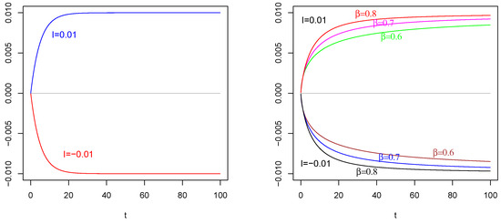
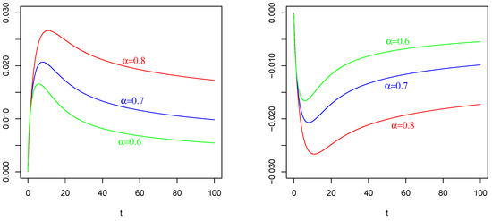
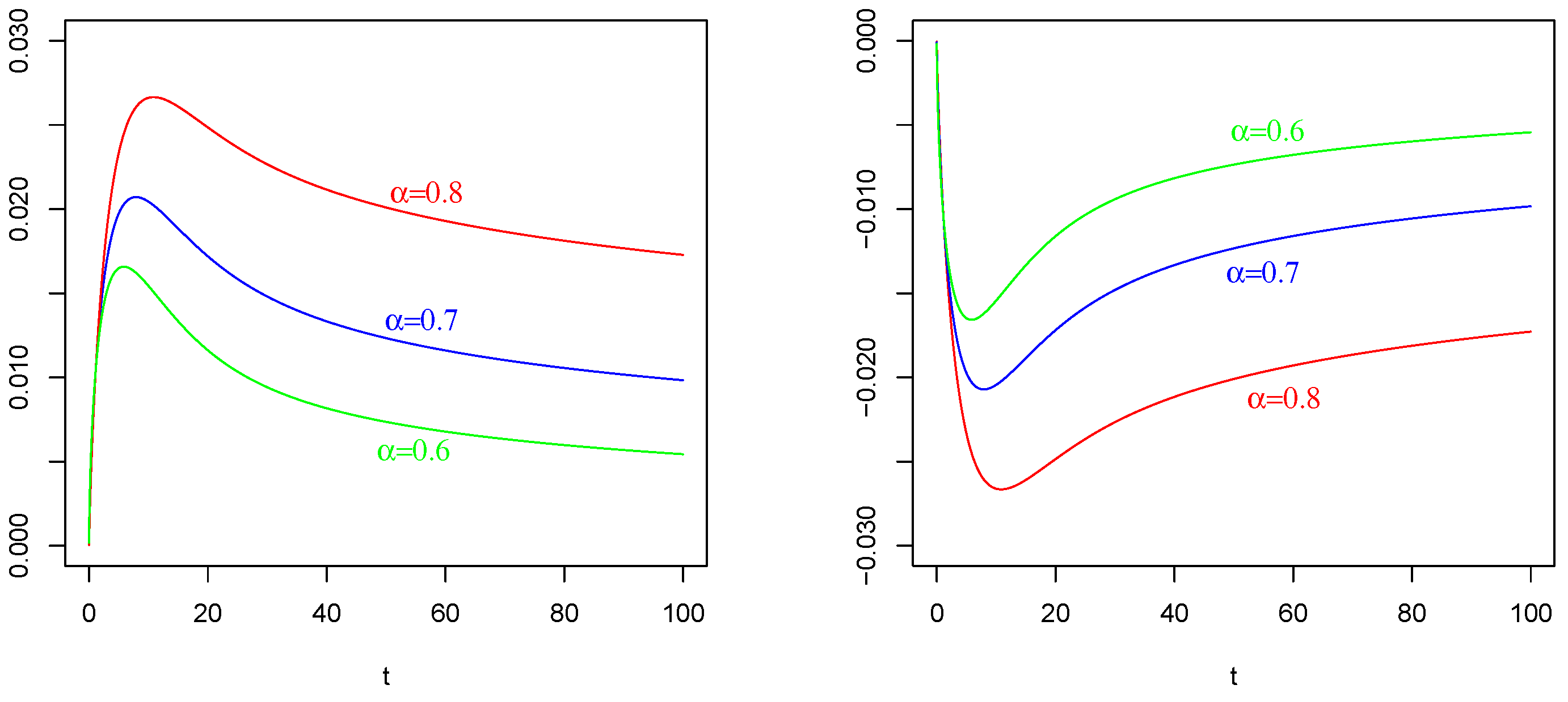
Figure 2. Mean of $V_1\left(t\right)$ as in (31) with $V_0=0,{\eta }_0=0$, $\varsigma =1,C_m=1,g_L=0.1$, $\tau =5$. On the (Left): $V_L=0.1$, $I=-0.01$, on the (Right) $V_L=-0.1$, $I=0.01$. The values of $\alpha$ are indicated in the figures.

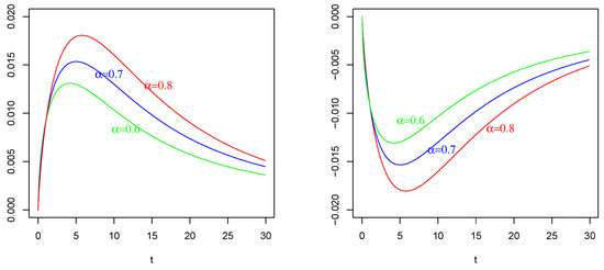
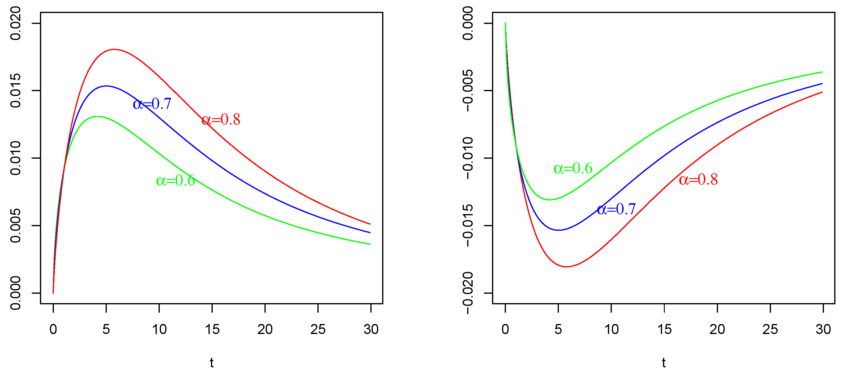
Figure 3. Mean of $V_2\left(t\right)$ as in (41) with $V_0=0,{\eta }_0=0$, $\sigma =1,C_m=1,g_L=0.1$, $\tau =5$. On the (Left): $V_L=0.1$, $I=-0.01$, on the (Right); $V_L=-0.1$, $I=0.01$. The values of $\alpha$ are indicated in the figures.

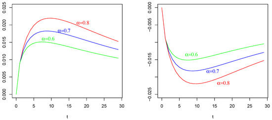
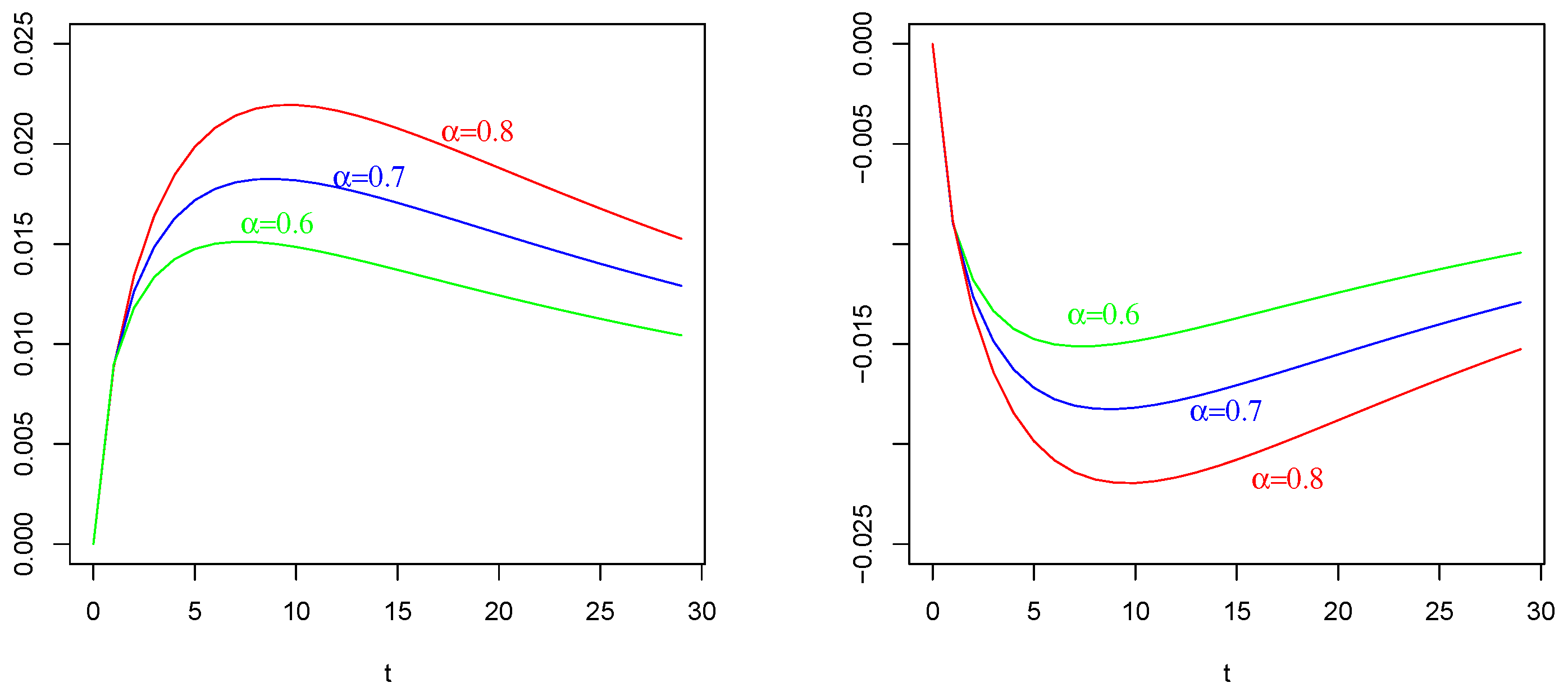
Figure 4. Mean of $V_3\left(t\right)$ as in (54) with $V_0=0,{\eta }_0=0$, $\sigma =1,C_m=1,g_L=0.1$, $\tau =5$ and $\beta =0.8$. On the (Left): $V_L=0.1$, $I=-0.01$, on the (Right): $V_L=-0.1$, $I=0.01$. The values of $\alpha$ are indicated in the figures.

In left side of Figure 1, we plot the mean of the input process as in (23) with ${\eta }_0=0$, $\tau =5$, for two values of current term $I.$ The red curve corresponds to an inhibitory current term $I=-0.01$, and the blue curve corresponds to an excitatory current term $I=0.01.$ Take into account the increasing (decreasing) behavior on time of the input correlated process $\eta \left(t\right)$ on the consequent change in the behavior of $V_1\left(t\right)$ (in Figure 2) and $V_2\left(t\right)$ (in Figure 3).

The effect of $\eta \left(t\right)$ (of Figure 1 Left) on $V_1\left(t\right)$ and $V_2\left(t\right)$: In contrast to the intuition, the negative current term $I=-0.01$ in the mean of $\eta \left(t\right)$ (the red curve) causes a positive depolarization (a peak) in the profiles of $V_1\left(t\right)$ and $V_2\left(t\right)$, as shown in Figure 2 Left and Figure 3 Left, respectively, for any considered values of fractional order $\alpha .$ A symmetrical behavior can be observed in the profiles of of $V_1\left(t\right)$ and $V_2\left(t\right)$, as shown in Figure 2 Right and Figure 3 Right, respectively, with a well (an hyper-polarization) in place of the peak, in correspondence of the positive current term $I=0.01$ in the mean of $\eta \left(t\right)$ (the blue curve in Figure 1 Left).

These results are also a consequence of the chosen value of the resting potential $V_L$, with opposite sign respect to the sign of the current term I; see the captions of Figure 2 and Figure 3, in which are specified the values of involved parameters, for details.

In the right side of Figure 1, we plot the mean of $\eta \left(t\right)$ as in (50) with ${\eta }_0=0$, $\tau =5$. The values of $\beta$ are indicated in the figure. For the positive current term $I=0.01$ in the mean (50) of $\eta \left(t\right)$, we plot the curves on top of Figure 1 Right. For the negative current term $I=-0.01$ in the mean (50) of $\eta \left(t\right)$, we plot the curves on bottom of Figure 1 Right.

The effect of $\eta \left(t\right)$ (of Figure 1 Right) with $\beta =0.8$ on $V_3\left(t\right)$: Again, in contrast with intuition, the negative current term $I=-0.01$ in the mean of $\eta \left(t\right)$ (the bottom curves) causes a positive depolarization (a peak, even if less sharp respect those in $V_1\left(t\right)$ and $V_2\left(t\right)$) in the profile of $V_3\left(t\right)$, as shown in Figure 4 Left, for any considered values of fractional order $\alpha .$ Symmetrically, the positive current term $I=0.01$ in the mean of $\eta \left(t\right)$ (the top curves) causes a hyper-polarization (a negative well) in the profile of $V_3\left(t\right)$, as shown in Figure 4 Right, for any considered values of fractional order $\alpha .$ Also, in this case, the chosen value of the resting potential $V_L$ played a determinant role in the behavior of the membrane process $V_3\left(t\right).$

Finally, we deduce that the effect of $\eta \left(t\right),$ corresponding to different stimuli modeled by I, on membrane processes $V_i\left(t\right),$ for $i=1,2,3,$ is more-or-less evident, and it can induce depolarization or hyper-polarization answers, when combined with some parameters of membrane processes, and in particular with the values of the resting potential.

Note that the choice of characteristic time $\tau =5$ for the $\eta \left(t\right)$ process is suggested by the comparison with the characteristic time $C_m/g_L=10$ of the membrane process $V_i\left(t\right).$ Indeed, we suppose that a less value for $\tau$ could have made less evident the effects on the membrane processes. Keeping this idea in mind, compare the time axis of Figure 1 with those of remaining figures: in such a way, it is possible to determine and compare the variation periods of these functions. This comment is given in order to underline that it is also possible to detect the persistence of the effect of input $\eta \left(t\right)$ on the membrane process.

Comparing Figure 2, Figure 3 and Figure 4

The mean functions of processes $V_1\left(t\right)$, $V_2\left(t\right)$ and $V_3\left(t\right)$ are plotted in Figure 2, Figure 3 and Figure 4, respectively, with all values of parameters as in Table 1. Specifically, we implemented R-scripts to obtain the plots of formulae (31), (41) and (54) for $V_1\left(t\right)$, $V_2\left(t\right)$ and $V_3\left(t\right)$, respectively. For the numerical evaluation of Mittag–Leffler functions, we uploaded the $MittagLeffleR$ R-package and used $integrate\left(\right)$ R-function for integral evaluations and vectorized $integrate\left(\right)$ for evaluating double integrals.

Plots in different colors are given for different values of the fractional order $\alpha .$ The left figures correspond to the case of a positive current I and a negative value of the resting potential $V_L.$ Vice versa, the right figures correspond to the case of a negative current I and a positive value of the resting potential $V_L.$

It is evident the different average behavior of the three processes $V_i\left(t\right)$ ($i=1,2,3$). We already commented on the effect of the input $\eta \left(t\right)$ of them, even if by comparing Figure 2, Figure 3 and Figure 4, the behaviors are different.

The effect of different fractional orders α: The main comment on these last Figures is related to the effect on the profiles of such means by varying the value of the fractional order $\alpha .$ We note that in all cases, i.e., in Figure 2, Figure 3 and Figure 4, the same ordering is observable. We refer to the ordering between the means of the same voltage process as $\alpha$ varies. The fact that in each case (and in each corresponding figure) the value $0.8$ of $\alpha$ determines the higher mean (or the lower one, in case of a negative sign) is justifiable by the use of the fractional integral of order $0.8$ able to preserve much more “łmemory” of the input effect and for much more time respect to cases corresponding to less fractional orders.

On the basis of this fact, we also adopted the value $0.8$ for the fractional order $\beta$ for the $\eta \left(t\right)$ process considered in Figure 4.

7. Concluding Remarks

In this contribution, a fractional model is proposed for neuronal dynamics essentially based on two coupled stochastic fractional differential Equations (1) and (2). In order to explain how the model can describe the biological phenomenon, some justifications are given in Section 2.

Note that we sometimes disregarded to specify the physical dimension of all involved functions and processes, but we remark that such specification, essential to apply the model, can be found in Table 1 for the re-scaled values, or in [18] for the original values.

We study the model on the basis of the mathematical setting given in Section 2.2; the explicit expressions of the processes, the means and covariances in the three different considered cases are given in Section 3, Section 4 and Section 5. These results show the rule played of the current term I, the correlated input $\eta \left(t\right)$, perturbed by a white noise, on the voltage process $V\left(t\right)$. We also provide figures with plots of means for $\eta \left(t\right)$ and $V\left(t\right)$ processes. The numerical results are studied and commented in detail. Hence, we try to clarify how some memory effects can be preserved and detected when such kind of models is applied.

Furthermore, this contribution is also particularly useful to design simulation algorithms with the purpose to obtain estimations for firing times by means of first passage time of these processes through the level $V_{th}$, the firing threshold. Our aim will be specialize simulation algorithms, in some cases already available, based on the generation of sample paths of Gaussian processes (see, for instance, [12,30]), but also to adopt and specialize other algorithms based on Euler–Maruyama schemes for stochastic fractional differential equation (see, for instance, [31]). Successive investigations about numerical and simulation approximations of FPTs for this model is mandatory and will be object of a future work.

References

- Podlubny, I. Fractional Differential Equations; Academic Press: New York, NY, USA, 1999. [Google Scholar]
- Samko, S.G.; Kilbas, A.A.; Marichev, O.I. Fractional Integrals and Derivatives: Theory and Applications; Gordon and Breach Science Publishers: Philadelphia, PA, USA, 1993. [Google Scholar]
- Ascione, G.; Mishura, Y.; Pirozzi, E. Fractional Deterministic and Stochastic Calculus; De Gruyter: Berlin, Germany, 2024. [Google Scholar]
- Benedetto, E.; Polito, F.; Sacerdote, L. On firing rate estimation for dependent interspike intervals. Neural Comput. 2015, 27, 699–724. [Google Scholar] [CrossRef]
- Kobayashi, R.; Kitano, K. Impact of slow K+ currents on spike generation can be described by an adaptive threshold model. J. Comput. Neurosci. 2016, 40, 347–362. [Google Scholar] [CrossRef] [PubMed]
- Stevens, C.F.; Zador, A.M. Novel integrate-and-fire-like model of repetitive firing in cortical neurons. In Proceedings of the 5th Joint Symposium on Neural Computation, San Diego, CA, USA, 16 May 1998; University of California: La Jolla, CA, USA, 1998; Volume 8, pp. 172–177. [Google Scholar]
- Tuckwell, H.C. Spatial neuron model with two-parameter Ornstein-Uhlenbeck input current. Phys. A Stat. Mech. Appl. 2006, 368, 495–510. [Google Scholar] [CrossRef]
- Burkitt, A.N. A review of the integrate-and-fire neuron model: I. Homogeneous synaptic input. Biol. Cybern. 2006, 95, 1–19. [Google Scholar] [CrossRef]
- Shinomoto, S.; Sakai, Y.; Funahashi, S. The Ornstein-Uhlenbeck process does not reproduce spiking statistics of cortical neurons. Neural Comput. 1997, 11, 935–951. [Google Scholar] [CrossRef] [PubMed]
- Bazzani, A.; Bassi, G.; Turchetti, G. Diffusion and memory effects for stochastic processes and fractional Langevin equations. Phys. A Stat. Mech. Appl. 2003, 324, 530–550. [Google Scholar] [CrossRef]
- Kim, H.; Shinomoto, S. Estimating nonstationary inputs from a single spike train based on a neuron model with adaptation. Math. Bios. Eng. 2014, 11, 49–62. [Google Scholar] [CrossRef] [PubMed]
- Abundo, M.; Pirozzi, E. Fractionally integrated Gauss-Markov processes and applications. In Communications in Nonlinear Science and Numerical Simulation; Elsevier: Amsterdam, The Netherlands, 2021; Volume 101, p. 105862. ISSN 1007-5704. [Google Scholar]
- Ascione, G.; Toaldo, B. A Semi-Markov Leaky Integrate-and-Fire model. Mathematics 2019, 7, 1022. [Google Scholar] [CrossRef]
- Pirozzi, E. On the Integration of Fractional Neuronal Dynamics Driven by Correlated Processes. In Computer Aided Systems Theory–EUROCAST 2019: Proceedings of the 17th International Conference, Las Palmas de Gran Canaria, Spain, 17–22 February 2019, Revised Selected Papers, Part I 17; Springer: Berlin/Heidelberg, Germany, 2020; pp. 211–219. [Google Scholar]
- Pirozzi, E. Colored noise and a stochastic fractional model for correlated inputs and adaptation in neuronal firing. Biol. Cybern. 2018, 112, 25–39. [Google Scholar] [CrossRef]
- Sakai, Y.; Funahashi, S.; Shinomoto, S. Temporally correlated inputs to leaky integrate-and-fire models can reproduce spiking statistics of cortical neurons. Neural Netw. 1999, 12, 1181–1190. [Google Scholar] [CrossRef]
- Teka, W.; Marinov, T.M.; Santamaria, F. Neuronal Spike Timing Adaptation Described with a Fractional Leaky Integrate-and-Fire Model. PLoS Comput. Biol. 2014, 10, e1003526. [Google Scholar] [CrossRef] [PubMed]
- Ascione, G.; Pirozzi, E. On a stochastic neuronal model integrating correlated inputs. Math. Biosci. Eng. 2019, 16, 5206–5225. [Google Scholar] [CrossRef] [PubMed]
- Baldi, P. Stochastic Calculus. In Universitext; Springer: Berlin/Heidelberg, Germany, 2017. [Google Scholar]
- Diethelm, K. The Analysis of Fractional Differential Equations. In Lecture Notes in Mathematics 2004; Springer: Berlin/Heidelberg, Germany, 2010. [Google Scholar]
- Ascione, G.; Pirozzi, E. Generalized Fractional Calculus for Gompertz-Type Models. Mathematics 2021, 9, 2140. [Google Scholar] [CrossRef]
- Burkitt A., N. A review of the integrate-and-fire neuron model: II. Inhomogeneous synaptic input and network properties. Biol. Cybern. 2006, 95, 97–112. [Google Scholar] [CrossRef] [PubMed]
- Wang, Y.; Xu, J.; Kloeden, P.E. Asymptotic behavior of stochastic lattice systems with a Caputo fractional time derivative. Nonlinear Anal. 2016, 135, 205–222. [Google Scholar] [CrossRef]
- Doan, T.S.; Kloeden, P.; Huong, P.; Tuan, H.T. Asymptotic separation between solutions of Caputo fractional stochastic differential equations. Stoch. Anal. Appl. 2018, 36, 654–664. [Google Scholar]
- Anh, P.T.; Doan, T.S.; Huong, P.T. A variation of constant formula for Caputo fractional stochastic differential equations. Stat. Probab. Lett. 2019, 145, 351–358. [Google Scholar] [CrossRef]
- Garrappa, R.; Kaslik, E.; Popolizio, M. Evaluation of Fractional Integrals and Derivatives of Elementary Functions: Overview and Tutorial. Mathematics 2019, 7, 407. [Google Scholar] [CrossRef]
- Li, K.; Peng, J. Laplace transform and fractional differential equations. Appl. Math. Lett. 2011, 24, 2019–2023. [Google Scholar]
- Kazem, S. Exact Solution of Some Linear Fractional Differential Equation by Laplace Transform. Int. J. Nonlinear Sci. 2013, 16, 3–11. [Google Scholar]
- Lansky, P. Sources of periodical force in noisy integrate-and-remodels of neuronal dynamics. Phys. Rev. E 1997, 55, 2040–2043. [Google Scholar] [CrossRef]
- Haugh, M. Generating Random Variables and Stochastic Processes; Monte Carlo Simulation; Columbia University: New York, NY, USA, 2017. [Google Scholar]
- Doan, T.S.; Huong, P.T.; Kloeden, P.E.; Vu, A.M. Euler–Maruyama scheme for Caputo stochastic fractional differential equations. J. Comput. Appl. Math. 2020, 380, 112989. [Google Scholar] [CrossRef]
Disclaimer/Publisher’s Note: The statements, opinions and data contained in all publications are solely those of the individual author(s) and contributor(s) and not of MDPI and/or the editor(s). MDPI and/or the editor(s) disclaim responsibility for any injury to people or property resulting from any ideas, methods, instructions or products referred to in the content. |
© 2024 by the author. Licensee MDPI, Basel, Switzerland. This article is an open access article distributed under the terms and conditions of the Creative Commons Attribution (CC BY) license (https://creativecommons.org/licenses/by/4.0/).