Multivariate Multiscale Higuchi Fractal Dimension and Its Application to Mechanical Signals

Abstract

Fractal dimension, as a common nonlinear dynamics metric, is extensively applied in biomedicine, fault diagnosis, underwater acoustics, etc. However, traditional fractal dimension can only analyze the complexity of the time series given a single channel at a particular scale. To characterize the complexity of multichannel time series, multichannel information processing was introduced, and multivariate Higuchi fractal dimension (MvHFD) was proposed. To further analyze the complexity at multiple scales, multivariate multiscale Higuchi fractal dimension (MvmHFD) was proposed by introducing multiscale processing algorithms as a technology that not only improved the use of fractal dimension in the analysis of multichannel information, but also characterized the complexity of the time series at multiple scales in the studied time series data. The effectiveness and feasibility of MvHFD and MvmHFD were verified by simulated signal experiments and real signal experiments, in which the simulation experiments tested the stability, computational efficiency, and signal separation performance of MvHFD and MvmHFD, and the real signal experiments tested the effect of MvmHFD on the recognition of multi-channel mechanical signals. The experimental results show that compared to other indicators, A achieves a recognition rate of 100% for signals in three features, which is at least 17.2% higher than for other metrics.

1. Introduction

Fractal theory is one of the three major nonlinear theories that originated in the early 19-th century. Fractal dimension (FD) is a branch of fractal theory that can be used to describe complex subjects such as non-smooth, non-regular, and scattered objects [1,2,3,4,5]. However, traditional FD metrics only take into account the complexity information of a single time scale when analyzing a time series, which cannot fully describe the complexity of the time series [6,7,8,9,10]. To overcome this shortcoming, in recent years, many scholars have used multiscale processing technology to improve the ability of FD to characterize the complexity of time series [11].

In 2018, Chen et al. combined multiscale processing techniques with the information dimension and proposed the multiscale information dimension, which comprehensively reflects the non-linear and non-smooth properties of the original time series [12]. Similar to the idea of multiscale information dimension, Yilmaz et al. proposed the multiscale Higuchi FD (HFD), inspired by multiscale sample entropy, which accurately identifies specific classes of random and chaotic time series [13]. Nevertheless, the above two multiscale FD only reflect the complexity of time series information in a single frequency band. To solve this problem, Li et al. proposed hierarchical refinement composite multiscale fractal dimension by introducing hierarchical analysis techniques to multiscale processing box dimensions, and the multiband characterization of complexity information was realized [14]. Yet, the above FD only considers data from a single channel of the time series, which cannot characterize the complexity information of a multichannel time series.

Similar to FD, sample entropy is a common non-linear dynamics metric that suffers from the inability to characterize multichannel time series information [15,16,17,18,19,20,21]. To overcome this problem, Ahmed and Mandic proposed multivariate multiscale sample entropy (MvmSE) for performing multiscale entropy analysis on multiple data channels simultaneously [22]. However, MvmSE is inaccurate in identifying multichannel short time series. To mitigate this shortcoming, multivariate multiscale fuzzy entropy (MvmFE) was proposed, which successfully characterizes the complexity information of short time series through fuzzy affiliation function properties [23]. Nevertheless, the first two entropy calculations take a long time and cannot obtain information on the magnitude of multichannel time series. To solve this problem, multivariate multiscale dispersion entropy (MvmDE) was proposed, which not only successfully reflects the complexity information of short time series but also calculates faster and considers the transformation of the magnitude of multichannel time series [24]. The results of the above studies show that multichannel information processing can help the above entropy-based metrics to successfully characterize the information of multichannel time series [25,26,27,28,29]. However, this multichannel information processing has not yet been applied to FD, and traditional FD still has the problem that it cannot characterize multivariate signals [30,31].

To solve this problem, multivariate HFD (MvHFD) is first proposed in this paper. Subsequently, to overcome the inability of MvHFD to reflect signal information at multiple time scales, multivariate multiscale HFD (MvmHFD) is then proposed. The main contributions of this paper are as follows: (i) MvHFD is proposed to solve the problem that traditional FD cannot reflect multichannel time series information via the utilization of multichannel information processing; (ii) to address the limitation that MvHFD cannot reflect time series information at different scales, MvmHFD is proposed to achieve a multichannel and multiscale representation of complexity; (iii) the validity of the proposed metrics is verified through simulation experiments, MvmHFD is successfully applied to multichannel mechanical signals, and the results show that MvmHFD is more effective than the other five entropy metrics in distinguishing different mechanical signals.

The rest of this paper is organized as follows: Section 2 introduces the theory of HFD, MvHFD, and MvmHFD; in Section 3, the validity of MvHFD and MvmHFD are verified via simulation experiments; Section 4 carries out multigroup comparison experiments on mechanical signals to demonstrate the advantages of MvmHFD; Section 5 draws conclusions.

2. Theory

2.1. Higuchi Fractal Dimension

HFD can measure the complexity of time series; if the time series is more complex, then the value of HFD is larger. Its specific calculation steps are shown below:

Step 1: Set a time series $X=\left\{x_i,i=1,2,\dots ,N\right\}$ of length $N$, and use the delay method to reconstruct the time series to obtain a matrix $X_k^m$, which is of the form:

$$X_k^m: X(m), X(m+k), X(m+2k), \dots , X(m+int\left(\frac{N-m}{k}\right)k)\hspace{1em}m=1,2,\dots ,k$$

(1)

where $k$ is the delay time and $m$ is the index of the starting point of each subsequence.

Step 2: Calculate the curve length $L_m(k)$ for each $X_k^m$, which can be obtained by Equation (2):

$$L_m\left(k\right)=\frac{1}{k}\left[\left(\sum _{i=1}^{int}|X(m+ik)-X(m+(i-1)k\left)\right|\right)\times \frac{N-1}{int\left(\frac{N-m}{k}\right)k}\right]$$

(2)

Step 3: Generate the mean value $L\left(k\right)$ of the curve length $L_m\left(k\right)$ of all sequences (matrices) $X_k^m$:

$$L\left(k\right)=\frac{1}{k}\sum _{m=1}^k{L}_m\left(k\right)$$

(3)

Step 4: Obtain a set of data on $k$ versus $L\left(k\right)$ for different values of $k$; plot the curve $lb(L(k))~lb(\frac{1}{k})$.

Step 5: Obtain the HFD values of the time series by fitting a straight line $lb\left(L\left(k\right)\right)=HFD\times lb\left(\frac{1}{k}\right)+C$; the value of HFD is the slope of the curve.

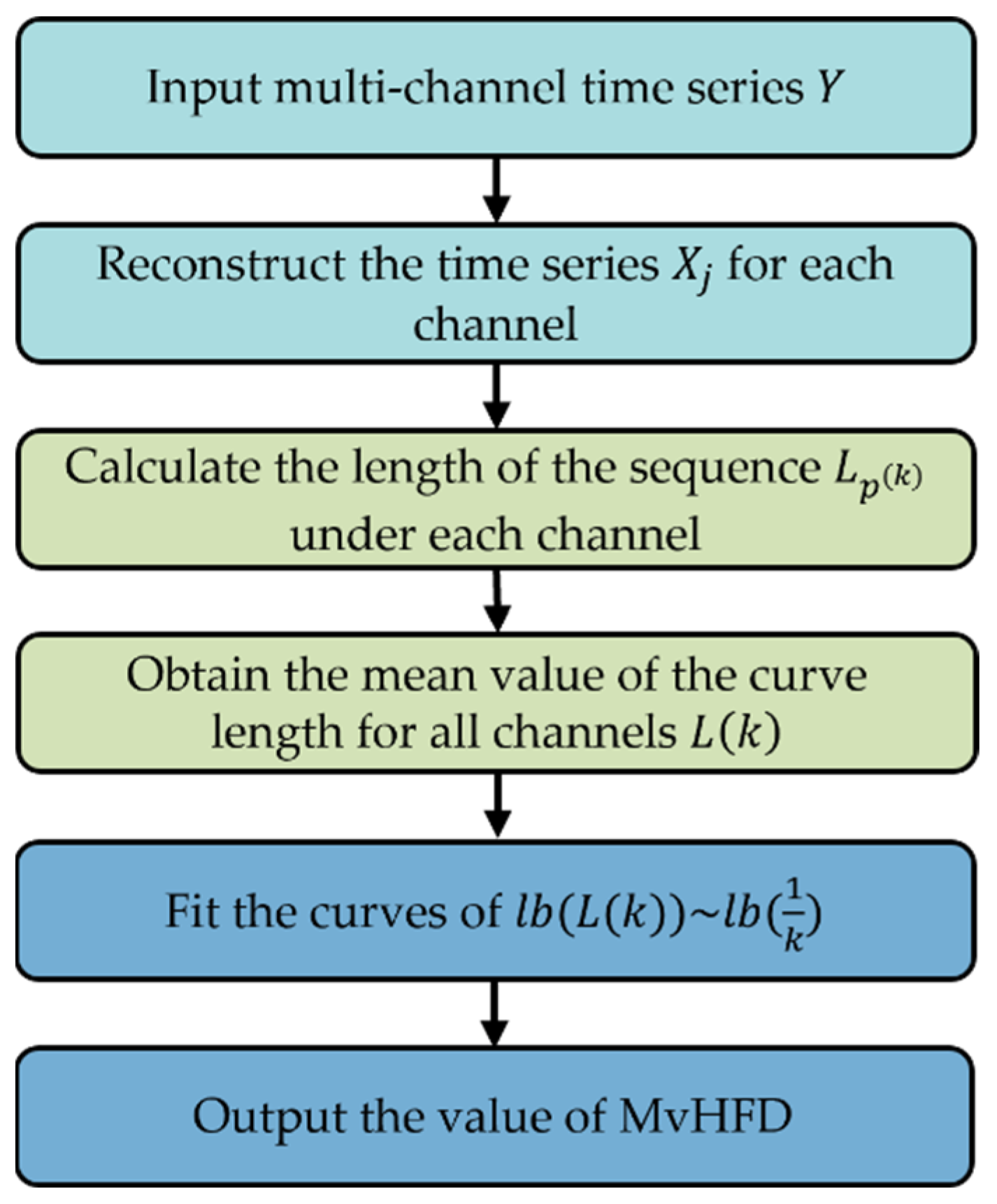
2.2. Multivariate Higuchi Fractal Dimension

Step 1: Transmit data from the $p$ -channels of the time series $Y=\left\{X_j,j=1,2,\dots ,p\right\}$. The data is transferred and the data from each channel are entered into Steps 1 through 3 of Section 2.1:

$$L_{p^{\left(k\right)}}=\frac{1}{k}\sum _{m=1}^k{L}_m^p(k)$$

(4)

where $k$ is the delay time, $L_{p^{\left(k\right)}}$ represents the length of the sequence curve for the channel of $p$ -th, and $L_m^p(k)$ is the length of ${X_j}_k^m$ under the $p$ -th channel.

$$L\left(k\right)=\frac{1}{p}\sum _{ii=1}^p{L}_{ii}\left(k\right) ii=1,2,\dots ,p$$

(5)

where $L\left(k\right)$ represents the average length of all channels.

Step 2: Enter $L\left(k\right)$ into Steps 4 through 6 of Section 2.1 to get the value of MvHFD.

$$lb\left(L\left(k\right)\right)=MvHFD\times lb\left(\frac{1}{k}\right)+C$$

(6)

where the value of HFD is the slope of the curve. Figure 1 shows the flowchart of MvHFD.

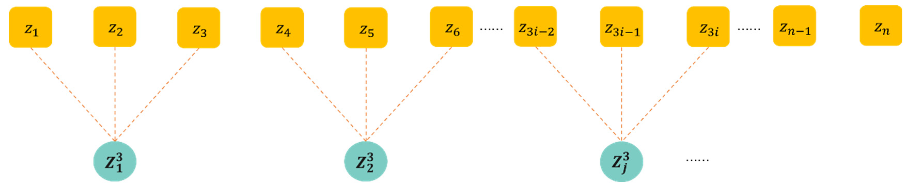
2.3. Multivariate Multiscale Higuchi Fractal Dimension

Step 1: The time series $Z=\left\{z_1,z_2,\dots ,z_N\right\}$ is divided into new subsequences by setting different scales:

$$z_j^{\left(s\right)}=\frac{1}{s}\sum _{\left(j-1\right)s+1}^{js}{z}_i, 1\le j\le \frac{N}{s}$$

(7)

where $s$ is the scale factor; significantly, the subsequence is the same as the original sequence when $s=1$.

Step 2: Each subsequence is fed into Section 2.2 to compute the value of MvmHFD:

$$MvmHFD\left(Z,s\right)=\frac{1}{s}\sum _{d=1}^{s}MvHFD\left(Z^{(s)}\right)$$

(8)

where $Z^{(s)}=\left\{z_1^{\left(s\right)},z_2^{\left(s\right)},\dots ,z_{\frac{N}{s}}^{\left(s\right)}\right\}$ is the sequence obtained after Equation (7) is performed at $Z^{(s)}$. To better illustrate the multiscale processing technology, we take $s=3$ as an example to display in Figure 2.

3. Analysis of Simulated Signals

The advantages of the proposed metrics are demonstrated by 3 perspectives, namely, stability, computational efficiency, and classification. The parameters of all metrics including MvHFD, multivariate dispersion entropy (MvDE), multivariate fuzzy entropy (MvFE), multivariate sample entropy (MvSE), multivariate permutation Lempel–Ziv complexity (MvPLZC) and multivariate dispersion entropy Lempel–Ziv complexity (MvDELZC) are shown in

Table 1. The parameter settings of the six metrics.

Parameter	Embedding Dimension	Delay Time	Threshold	Number of Categories
MvHFD	-	20	-	- -
MvDE	3	1	-	- 6
MvFE	2	1	0.15	- -
MvSE	2	1	0.15	- -
MvPLZC	3	1	-	- -
MvDELZC	3	1	-	6

. MvHFD differs from other metrics in that all other metrics have a fixed range of recommended parameters, while the delay time range of MvHFD is not fixed. In this paper, the delay time of MvHFD was set to 20.

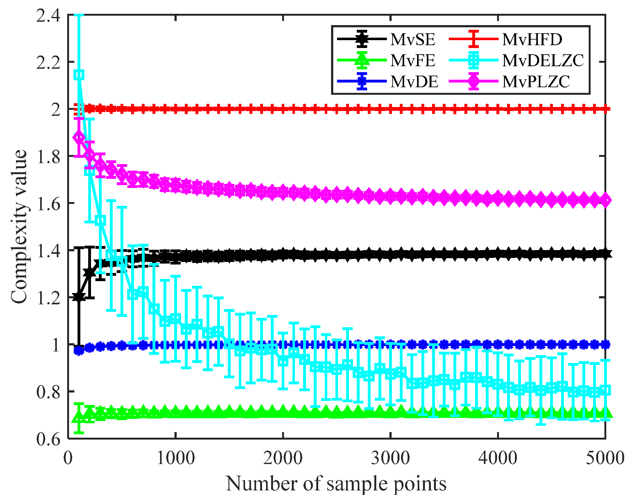
3.1. Stability Testing Experiment

We used 3-channel white noise to test the stability of MvHFD, where the length of the first sample of each channel for white noise was 100 sample points, the length of the second sample was 200 sample points, and so on. The remaining samples were increased sequentially to 5000 by increasing the length by 100 sample points each time for a total of 50 samples, and the length of the 50th sample was 5000. Figure 3 demonstrates the mean and standard deviation of six metrics at different data lengths.

From Figure 3, as the length of the number of samples increased, the trend in the complexity of all the metrics could be seen, with MvDE and MvFE increasing first and then remaining unchanged, MvDELZC and MvPLZC continuing to decrease, and MvHFD always remaining the same. The complexity values of all the metrics were stable for sample lengths greater than 3000 sample points; at sample lengths greater than 1000, the complexity of MvPLZC and MvDELZC decreased with increasing sample length, and the complexity values of the remaining metrics held essentially constant as the sample length increased. It can be concluded that compared to the remaining metrics, MvFE and MvHFD had the most stable complexity values with increasing sample length.

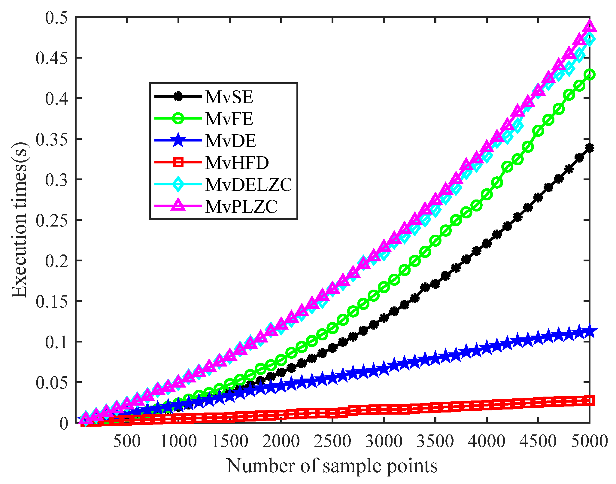
3.2. Computational Efficiency Testing Experiment

We utilized three-channel white noise to test the computational efficiency of the proposed metrics with the same sample length data taken as in Section 3.1. The simulations were carried out using a PC with Gen Intel(R) Core (TM), i9-13900HX, 2.2 GHz and 16 GB RAM by MATLAB R2022b, and the execution time was the mean of 1000 computation times for each sample length. Figure 4 demonstrates the execution times of the various metrics at different data lengths.

From Figure 4, it can be observed that the execution times of all the metrics increased with the increase of sample length; among them, the computation time of MvHFD was always the smallest. Additionally, MvDELZC and MvPLZC had the highest computing cost. For the metrics of MvSE, MvFE and MvDE, the computation time of the three methods was basically the same when the number of samples was less than 1500; when the number of samples was more than 1500, MvFE was the slowest and MvDE was the fastest. Therefore, it can be concluded that compared with other metrics, MvHFD had the shortest calculation time and the highest efficiency under the same sample point length.

3.3. Classification Ability Testing Experiment

Pink noise, white noise, and red noise are used in this section to test the capability of the proposed metrics for discriminating signals. There were three channels for each signal, where 204,800 sample points were obtained for every channel and 100 samples were used with an overlap rate of 0; each sample had 2048 sample points. Figure 5 shows the mean and standard deviation of the complexity of the six metrics, including the MvmHFD, MvmDE, MvmSE, MvmSE, MvmFE, multivariate permutation Lempel–Ziv complexity (MvmPLZC), and multivariate multiscale dispersion entropy Lempel–Ziv complexity (MvmDELZC) for three noise signals at ten scales.

As can be seen from Figure 5, for each scale, MvmHFD was able to distinguish three noise signals and MvmPLZC and MvmDELZC were able to differentiate red noise, while MvmDE, MvmSE, and MvmFE were unable to discriminate three noise signals; MvmDE, MvmSE, and MvmFE were able to differentiate three noise signals at a scale of 1, and were able to distinguish white noise from a scale 6 to 10. MvmHFD and MvmDE had the smallest standard deviation, while MvmPLZC and MvmDELZC had the largest standard deviation. Therefore, it can be concluded that MvmHFD shows stronger signal discrimination than other metrics.

4. Analysis of Real Signals

We used the eight-channel mechanical signals of [32] to test the differentiation ability of MvmHFD for signals, and the parameters of each metric were set to be the same as in Section 3 at a scale of 10. Section 4.1 and Section 4.2 concern the bearing and gear signals, respectively.

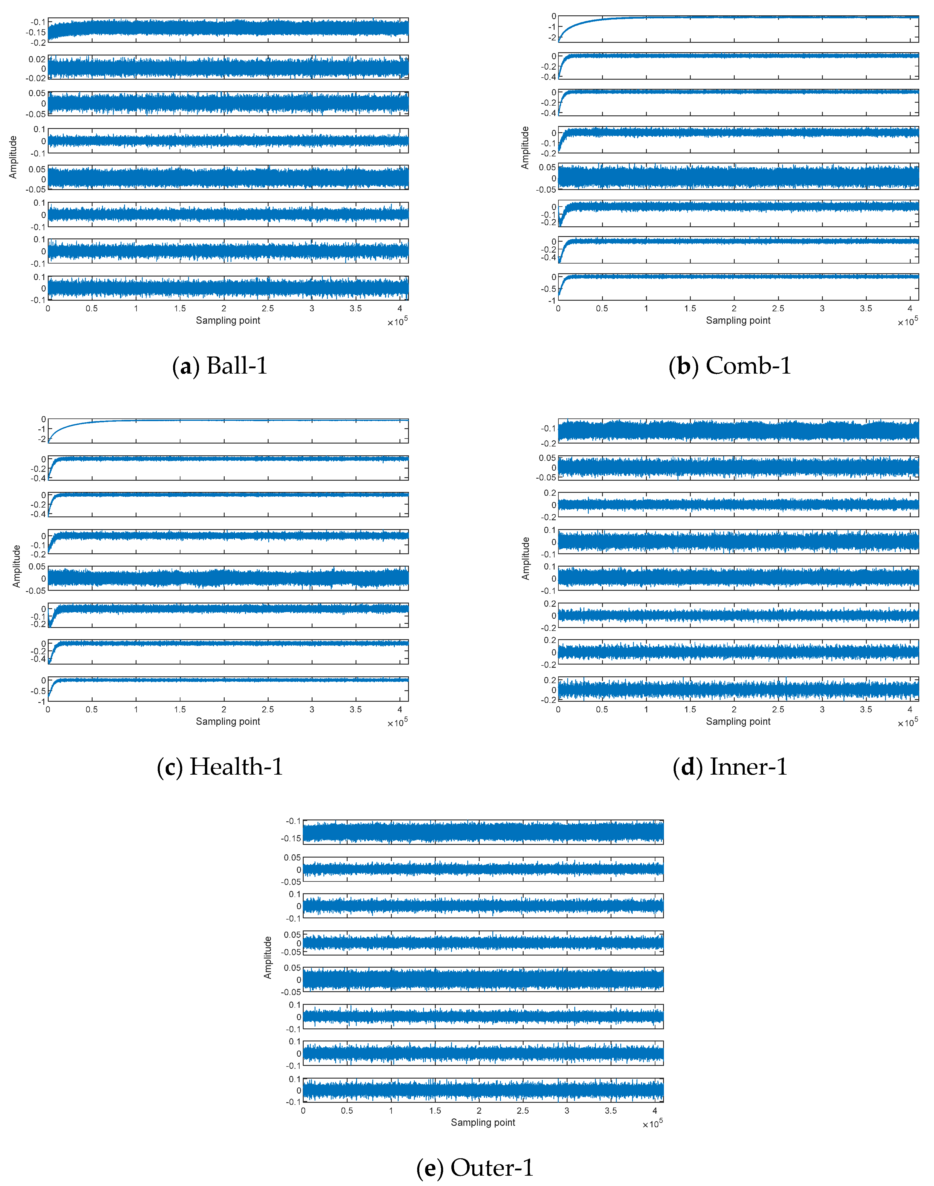
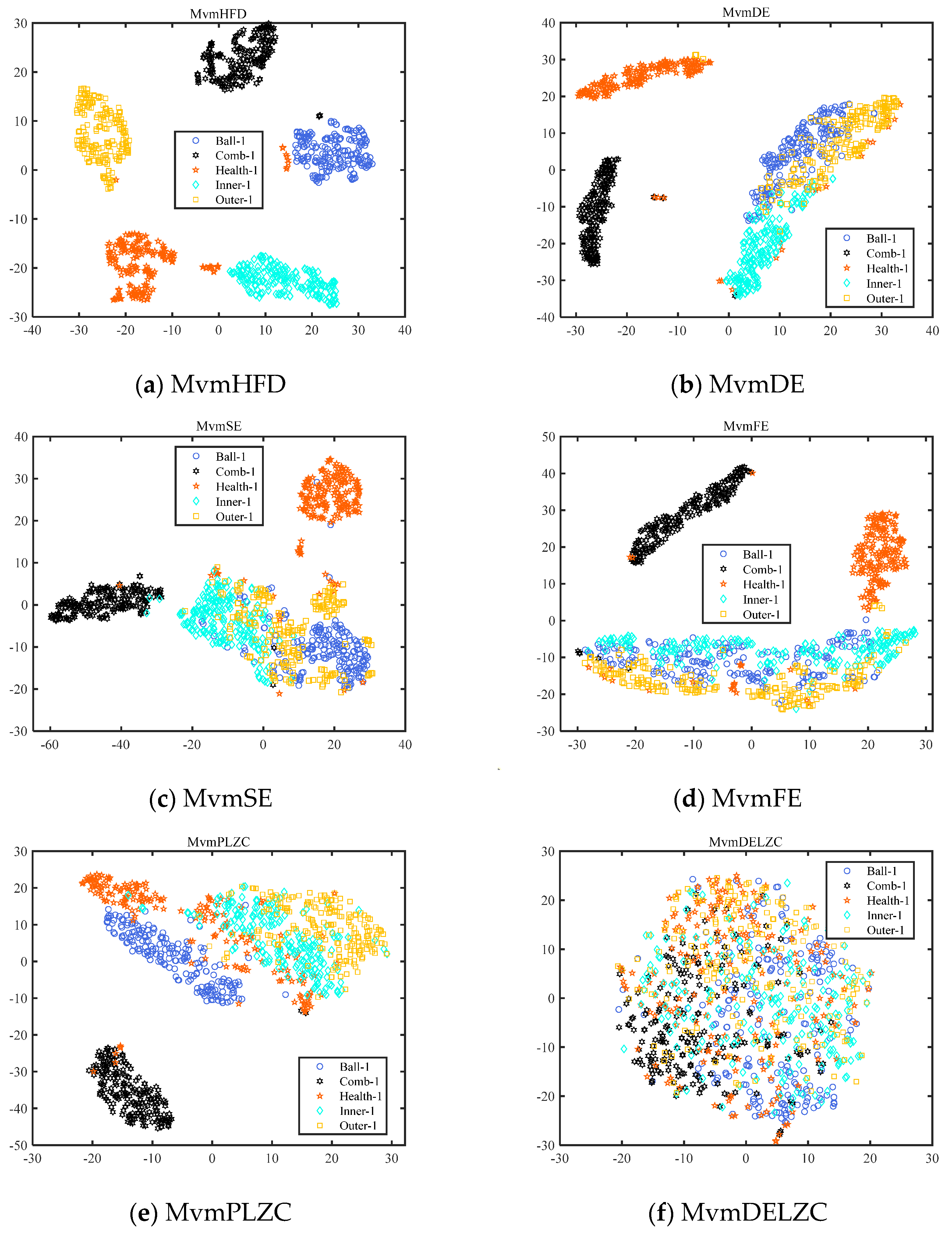
4.1. Real Bearing Signal Differentiation Experiment

The bearing signal data used in this section included the ball fault, combination fault, health state, inner ring fault and outer ring fault, all of which are eight-channel bearing signals. We named these signals Ball-1, Comb-1, Health-1, Inner-1, and Outer-1. Each channel was selected for the first 409,600 sampling points, which were evenly divided into 200 samples without overlapping parts, with each sample containing 2048 sampling points. Figure 6 shows the eight-channel time-domain waveforms for the five bearing signals, and each sub-figure shows channels one to eight from top to bottom.

To visualize the ability of this metric to distinguish bearing signals, t-Distributed Stochastic Neighbor Embedding (T-SNE) [33] was utilized to demonstrate the feature distribution, which is able to map 10-dimensional data onto a 2-dimensional plane. The 10-dimensional data of T-SNE represents the complexity features of bearing signals at ten different scales. Figure 7 illustrates the T-SNE map of the six metrics for the five bearing fault signals.

As seen from Figure 7, none of the metrics were able to distinguish the five bearing signals perfectly; MvmDELZC mixed all the samples from all the signals into a cluster, MvmDE had all the samples from three type of signals mixed together; MvmDE, MvmSE, and MvmFE only had one type of signal separated from the other signals; and MvmHFD could not distinguish the five bearing signals. The clustering of samples for each signal was most excellent. Therefore, it can be concluded that MvmHFD is more capable of distinguishing the five bearing signals than the other metrics.

To further compare the discriminative ability of MvmHFD for the five types of bearing signals, we demonstrate the recognition effect of MvmHFD on signals from two aspects: different scales and different quantities of feature extraction.

Table 2. The ARR of the six metrics for the five bearing fault signals at different scales (%).

Metric	Different Scales										ARR
	1	2	3	4	5	6	7	8	9	10
MvmHFD	83.0	70.2	56.4	63.0	70.4	72.8	55.4	56.2	77.4	69.8	67.36
MvmDE	41.0	42.8	63.0	59.8	59.6	57.0	54.4	53.8	49.6	53.0	53.40
MvmFE	48.0	51.2	5.08	59.8	55.6	49.0	50.6	49.0	50.4	51.0	46.97
MvmSE	35.4	38.4	48.0	48.8	49.8	51.0	53.4	48.0	48.8	49.8	47.14
MvmPLZC	40.8	26.8	24.4	35.4	42.4	43.4	40.2	41.8	42.6	44.4	38.22
MvmDELZC	28.4	21.6	23.0	19.8	20.2	19.4	20.8	20.6	24.6	20.0	21.84

states the average recognition rate (ARR) of the six metrics for the five bearing fault signals at different scales, in which ARR is the mean of the recognition rates at ten scales.

Table 3. The ARR of the six metrics for the five bearing signals with different numbers of extracted features (%).

Metric	Number of Extracted Features
	2	3	4	5	6	7	8	9	10
MvmHFD	97.8	100	100	100	100.0	100.0	100	100	100
MvmDE	73.0	82.8	82.2	82.6	82.4	82.2	83.0	82.2	80.8
MvmFE	67.6	72.4	74.6	74.6	75.2	76.2	75.2	74.2	73.8
MvmSE	76.0	82.0	83.8	82.8	82.8	82.0	81.8	81.2	80.6
MvmPLZC	68.2	75.6	78.0	80.0	81.4	82.8	83.6	83.4	82.2
MvmDELZC	32.4	35.6	38.2	40.8	41.6	41.6	39.4	38.4	39.6

shows the ARR of the six metrics for the five bearing signals with different numbers of extracted features.

According to Table 2, the ARR of the bearing signals under the ten scales was highest for MvmHFD and lowest for MvmDELZC; MvmHFD had the highest recognition rate under nine scales and MvmDE had the highest recognition rate under the third scale; the recognition rate of MvmHFD exceeded 70% at five scales, and its recognition rate under the first scale reached 83%, which is at least 30% higher than the highest recognition rate of the other scales. It can be concluded that MvmHFD has a good differentiation effect on the five bearing signals under a single feature, and that the ARR is much higher than the other metrics.

From Table 3, it can be seen that in the transition of all the metrics from the single-feature method to the double-feature method, the greatest improvement was shown in the recognition rate; MvmHFD had the highest recognition rate for the five bearing signals regardless of the number of features, and the recognition rate even reached 100% when the number of features was greater than or equal to three. With the exception of MvmHFD, the recognition rate of the remaining metrics for the five bearing signals increased first and then decreased with increases in the number of features. In conclusion, the multiple feature approach for all metrics was better than the single feature approach for distinguishing the five kinds of bearing signals, and MvmHFD had the highest recognition effect for the five kinds of bearing signals, regardless of the number of features.

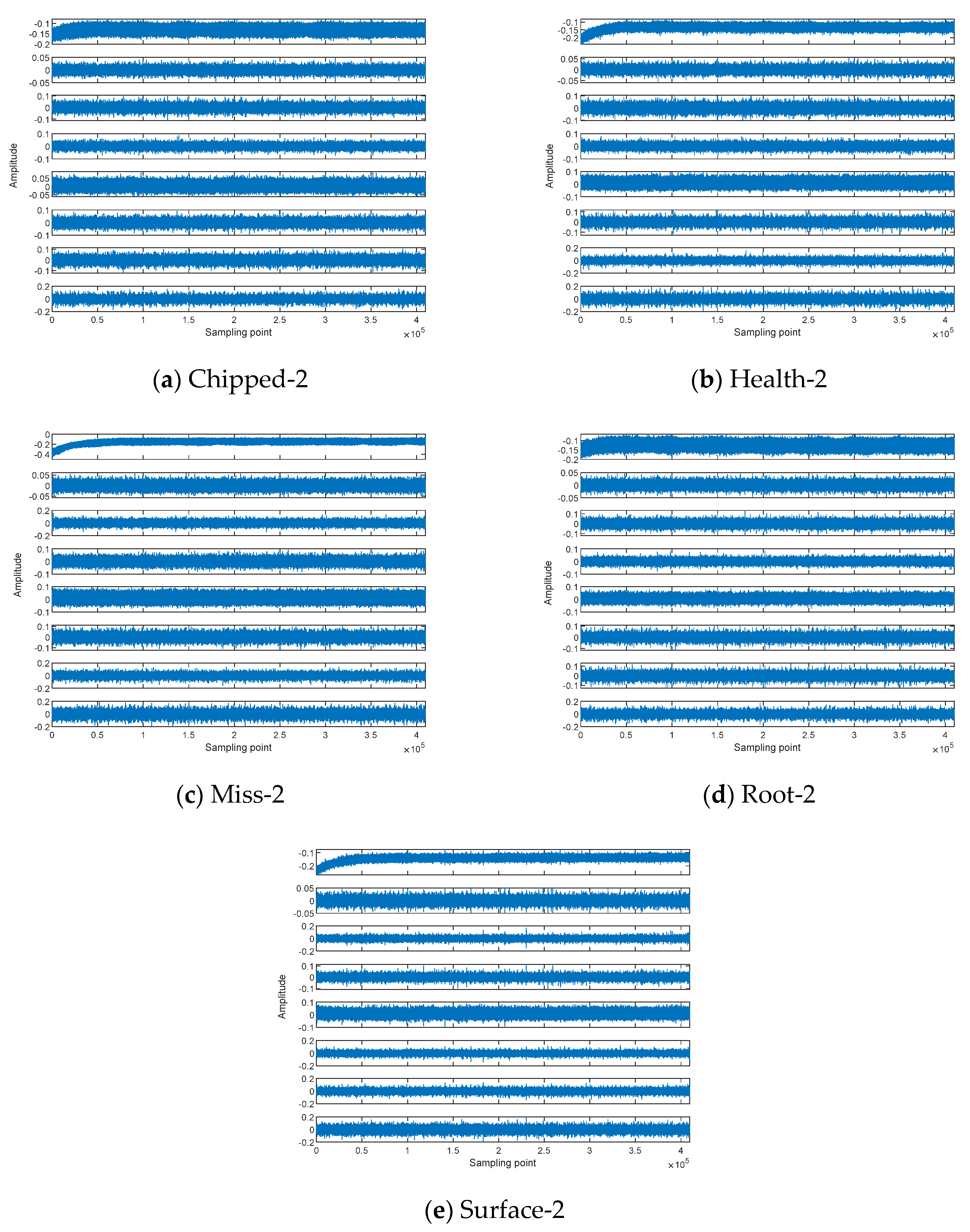
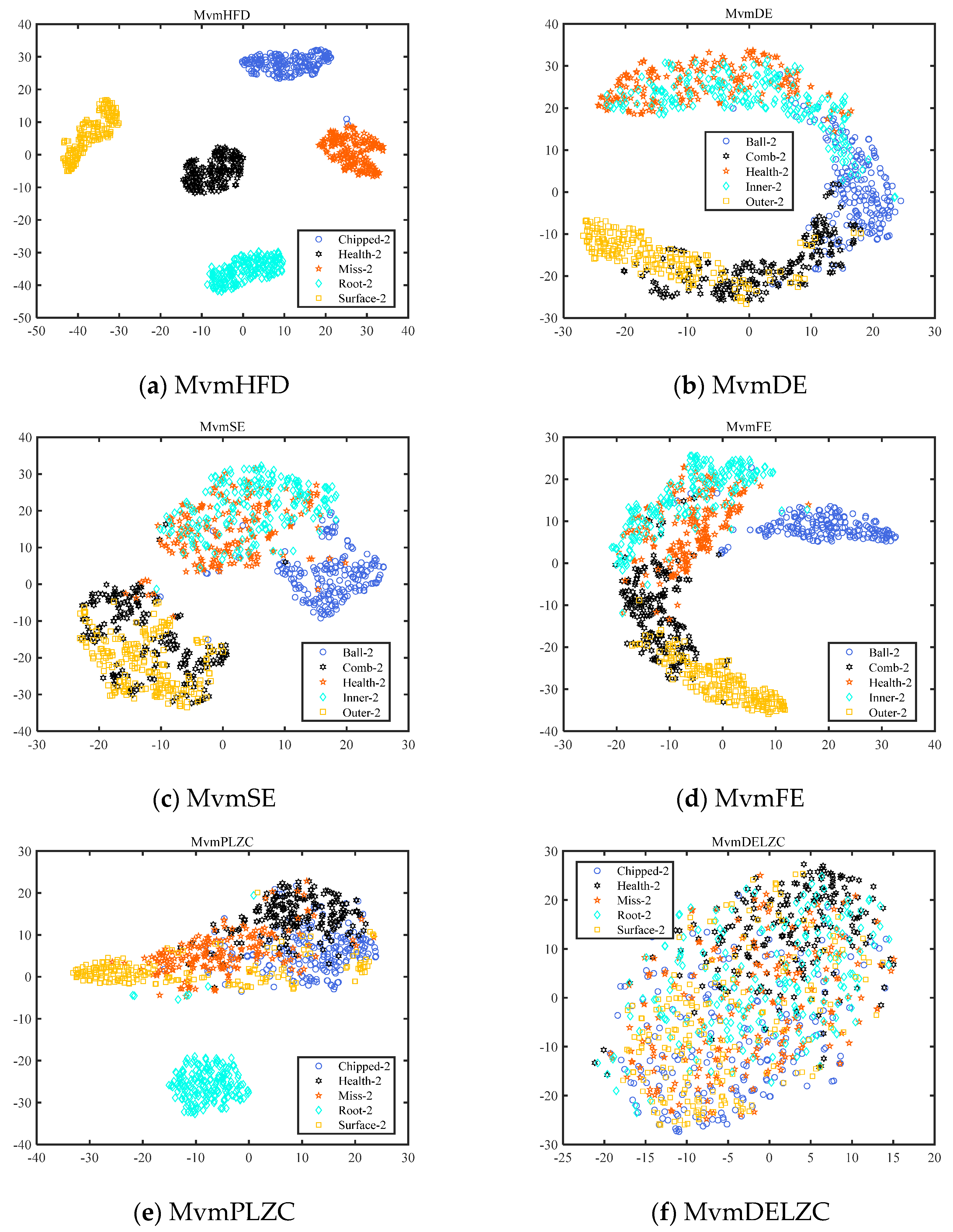
4.2. Real Gear Signal Differentiation Experiment

The gear signals used in this section included the chipped fault, health state, miss fault, root fault and surface fault, covering all eight channels of data. These signals were named Chipped-2, Health-2, Miss-2, Root-2, and Surface-2. The data selection for each channel was the same as in Section 4.1, and Figure 8 shows the eight-channel time-domain waveforms for the five gear signals.

As in Section 4.1, we used T-SNE to map 10-dimensional data onto a 2-dimensional plane; the 10-dimensional data represents the complexity features of gear signals at ten different scales. Figure 9 illustrates the T-SNE map of the six metrics for the five gear signals.

From Figure 9, it can be seen that there were no metrics that could completely distinguish the five gear signals; for MvmDE and MvmDELZC, the samples of all the signals overlapped together and had the worst aggregation. The distribution of MvmSE, MvmFE, and MvmPLZC was divided into two parts; each of the signals of the MvmHFD was separated into separate clumps and only two Chipped-2 samples were mixed with Miss-2. It can be concluded that MvmHFD had the best clustering and differentiation effect on the five gear signals compared to the other metrics.

Similar to Section 4.1,

Table 4. The ARR of the six metrics for the five gear signals at different scales (%).

Metric	Different Scales										ARR
	1	2	3	4	5	6	7	8	9	10
MvmHFD	89.8	63.4	71.2	50.2	62.0	61.4	65.4	73.2	63.8	58.4	65.88
MvmDE	28.2	40.2	40.2	48.0	48.0	57.0	57.8	56.8	51.0	56.4	48.36
MvmFE	23.8	41.6	43.2	49.0	50.6	56.4	55.8	59.2	55.2	55.8	49.06
MvmSE	24.2	39.0	45.4	45.6	44.8	42.0	44.8	40.8	33.4	42.8	40.28
MvmPLZC	22.2	31.2	25.8	29.2	35.0	31.0	29.0	27.8	26.4	24.8	28.24
MvmDELZC	25.6	23.6	25.4	22.6	23.8	22.0	24.0	24.6	21.2	23.6	23.64

illustrates the ARR of the six metrics for the five gear signals at different scales. The ARR of the six metrics for the five gear signals with different numbers of extracted features is shown in

Table 5. The ARR of the six metrics for the five gear signals with different numbers of extracted features (%).

Metric	Number of Extracted Features
	2	3	4	5	6	7	8	9	10
MvmHFD	99.4	100	100	100	100	100	100	100	100
MvmDE	67.8	70.2	72.4	74.2	74.2	73.6	72.2	71.2	69.2
MvmFE	71.6	77.6	80.4	80.8	81.6	82.0	82.6	82.2	83.0
MvmSE	66.8	70.2	74.2	75.0	74.6	75.6	75.4	73.6	73.4
MvmPLZC	53.0	66.8	71.0	73.0	74.8	76.0	76.4	75.6	74.0
MvmDELZC	30.6	34.2	33.4	33.2	35.0	34.0	33.4	34.2	31.4

.

From Table 4, except for MvmHFD, the recognition rate of the remaining metrics for the five gear signals did not exceed 60% at each scale; the ARR of MvmHFD for the five gear signals reached a maximum of 65.88%, and the recognition rate reached a maximum of 89.8% in the first scale; the ARR of MvmDELZC for the five gear signals reached a minimum of only 23.64%, and the lowest recognition rate of 21.2% at the ninth scale. It can be concluded that MvmHFD has the highest recognition rate for multichannel gear signals compared to other metrics.

From Table 5, it can be seen that the use of multiple feature improved the recognition rate significantly more than the single feature method; the recognition rate of MvmHFD with increasing numbers of features first increased and then remained unchanged once it reached 100%; the recognition rate of MvmFE increased consistently with increases in the number of features; with the exception of MvmHFD and MvmFE, the remaining metrics first increased and then decreased in recognition rate as the number of features increased. In conclusion, compared with other metrics, the MvmHFD-based multiple feature extraction method had the highest recognition rate for the five gear signals and had the best ability to distinguish signals.

5. Conclusions

Two improved FD metrics, MvHFD and MvMHFD, were proposed from both the multiscale and multichannel perspectives. The effectiveness of the proposed metrics was verified through simulations and real mechanical signal experiments. The main conclusions can be summarized as follows:

(1)

The use of MvHFD was proposed by introducing multichannel information processing, which realizes multichannel representation for the complexity of time series. MvmHFD, as an improvement of MvHFD, was proposed via the use of multiscale processing technology that achieves dual complexity characterization for multichannel and multiscale information.

(2)

The superiority of the proposed metric was verified by three sets of simulation experiments. The experimental results showed that MvHFD had the best stability and high computational efficiency, and MvmHFD had the strongest signal discrimination capability.

(3)

Two groups of real signals were used to test the effectiveness of MvmHFD, and the experimental results showed that MvmHFD had a stronger ability to discriminate mechanical signals than other metrics with each number of features, and the recognition rate reached 100% under multiple features, which is at least 16.4% higher than other metrics.

References

1. Mandelbrot, B. How long is the coast of Britain? Statistical self-similarity and fractal dimension. Science 1967, 156, 636–638. [Google Scholar] [CrossRef] [PubMed]
2. Mandelbrot, B. Les Objects Fractals: Forme Hasard et Dimension; Flammarion: Paris, France, 1975. [Google Scholar]
3. Mandelbrot, B. Fractal Object: Form, Chance and Dimension; Freeman: San Francisco, CA, USA, 1977. [Google Scholar]
4. Li, Y.; Zhou, Y.; Jiao, S. Variable-Step Multiscale Katz Fractal Dimension: A New Nonlinear Dynamic Metric for Ship-Radiated Noise Analysis. Fractal Fract. 2024, 8, 9. [Google Scholar] [CrossRef]
5. Li, Y.; Tang, B.; Jiao, S.; Su, Q. Snake Optimization-Based Variable-Step Multiscale Single Threshold Slope Entropy for Complexity Analysis of Signals. IEEE Trans. Instrum. Meas. 2023, 72, 6505313. [Google Scholar] [CrossRef]
6. Higuchi, T. Approach to an irregular time series on the basis of the fractal theory. Phys. D Nonlinear Phenom. 1988, 31, 277–283. [Google Scholar] [CrossRef]
7. Mayor, D.; Steffert, T.; Datseris, G.; Firth, A.; Panday, D.; Kandel, H.; Banks, D. Complexity and Entropy in Physiological Signals (CEPS): Resonance Breathing Rate Assessed Using Measures of Fractal Dimension, Heart Rate Asymmetry and Permutation Entropy. Entropy 2023, 25, 301. [Google Scholar] [CrossRef] [PubMed]
8. Matteo, B.; Corrado, C.; Ausilia, V.; Caterina, P.; Beatrice, V.; Cristian, Z.; Luca, C.; Emiliano, S.; Marco, B.; Giuseppe, D. Motor unit synchronization and firing rate correlate with the fractal dimension of the surface EMG: A validation study. Chaos Solitons Fractals 2023, 167, 113021. [Google Scholar]
9. Li, Y.; Jiao, S.; Deng, S.; Geng, B.; Li, Y. Refined composite variable-step multiscale multimapping dispersion entropy: A nonlinear dynamical index. Nonlinear Dyn. 2023. [Google Scholar] [CrossRef]
10. Gagnepain, J.; RoQues-Carmes, C. Fractal approach to two dimensional and three dimensional surface roughness. Wear 1986, 109, 119–126. [Google Scholar] [CrossRef]
11. Li, Y.; Zhang, S.; Liang, L. Variable-step multi-scale fractal dimension and its application to ship radiated noise. Ocean Eng. 2023, 286, 115573. [Google Scholar] [CrossRef]
12. Chen, X.; Peng, L.; Cheng, G.; Luo, C. Research on Degradation State Recognition of Planetary Gear Based on Multiscale Information Dimension of SSD and CNN. Complexity 2019, 2019, 8716979. [Google Scholar] [CrossRef]
13. Yilmaz, A.; Unal, G. Multiscale Higuchi’s fractal dimension method. Nonlinear Dyn. 2020, 101, 1441–1455. [Google Scholar] [CrossRef]
14. Li, Y.; Liang, L.; Zhang, S. Hierarchical Refined Composite Multi-Scale Fractal Dimension and Its Application in Feature Extraction of Ship-Radiated Noise. Remote Sens. 2023, 15, 3406. [Google Scholar] [CrossRef]
15. Richman, J.S.; Moorman, J.R. Physiological time series analysis using approximate entropy and sample entropy. Am. J. Physiol. Heart Circ. Physiol. 2000, 278, 2039–2049. [Google Scholar] [CrossRef] [PubMed]
16. Chou, L.; Gong, S.; Yang, H.; Liu, J.; Chou, Y. A fast sample entropy for pulse rate variability analysis. Med. Biol. Eng. Comput. 2023, 61, 1603–1617. [Google Scholar] [CrossRef] [PubMed]
17. Zheng, J.; Li, Y.; Zhai, Y.; Zhang, N.; Yu, H.; Tang, C.; Yan, Z.; Luo, E.; Xie, K. Effects of sampling rate on multiscale entropy of electroencephalogram time series. Biocybern. Biomed. Eng. 2023, 43, 233–245. [Google Scholar] [CrossRef]
18. Guilherme, B.; Marcelo, Z.; Guilherme, F.; Paulo, R.; Adriano, B.; Thaína, A.; Leandro, A. Classification of non-Hodgkin lymphomas based on sample entropy signatures. Expert Syst. Appl. 2022, 202, 117238. [Google Scholar]
19. Song, Y.; Crowcroft, J.; Zhang, J. Automatic epileptic seizure detection in EEGs based on optimized sample entropy and extreme learning machine. J. Neurosci. Methods 2012, 210, 132–146. [Google Scholar] [CrossRef]
20. Alcaraz, R.; Rieta, J.J. Sample entropy of the main atrial wave predicts spontaneous termination of paroxysmal atrial fibrillation. Med. Eng. Phys. 2009, 31, 917–922. [Google Scholar] [CrossRef]
21. Delgado-Bonal, A.; Marshak, A. Approximate Entropy and Sample Entropy: A Comprehensive Tutorial. Entropy 2019, 21, 541. [Google Scholar] [CrossRef]
22. Ahmed, M.U.; Mandic, D.P. Multivariate multiscale entropy: A tool for complexity analysis of multichannel data. Phys. Rev. E 2011, 84, 061918. [Google Scholar] [CrossRef]
23. Ahmed, M.U.; Chanwimalueang, T.; Thayyil, S.; Mandic, D. A Multivariate Multiscale Fuzzy Entropy Algorithm with Application to Uterine EMG Complexity Analysis. Entropy 2017, 19, 2. [Google Scholar] [CrossRef]
24. Azami, H.; Fernández, A.; Escudero, J. Multivariate Multiscale Dispersion Entropy of Biomedical Times Series. Entropy 2019, 21, 913. [Google Scholar] [CrossRef]
25. Yang, Y.; Zheng, H.; Yin, J.; Xu, M.; Chen, Y. Refined composite multivariate multiscale symbolic dynamic entropy and its application to fault diagnosis of rotating machine. Measurement 2020, 151, 107233. [Google Scholar] [CrossRef]
26. Zhang, N.; Lin, A.; Ma, H.; Shang, P.; Yang, P. Weighted multivariate composite multiscale sample entropy analysis for the complexity of nonlinear times series. Phys. A Stat. Mech. Its Appl. 2018, 508, 595–607. [Google Scholar] [CrossRef]
27. Yin, Y.; Shang, P. Multivariate multiscale sample entropy of traffic time series. Nonlinear Dyn. 2016, 86, 479–488. [Google Scholar] [CrossRef]
28. Zhang, Y.; Shang, P. Multivariate multiscale distribution entropy of financial time series. Phys. A Stat. Mech. Its Appl. 2019, 515, 72–80. [Google Scholar] [CrossRef]
29. Yin, Y.; Shang, P. Multivariate weighted multiscale permutation entropy for complex time series. Nonlinear Dyn. 2017, 8, 1707–1722. [Google Scholar] [CrossRef]
30. Coelho, A.; Lima, C. Assessing fractal dimension methods as feature extractors for EMG signal classification. Eng. Appl. Artif. Intell. 2014, 36, 81–98. [Google Scholar] [CrossRef]
31. Hu, J.; Tung, W.; Gao, J. Detection of low observable targets within sea clutter by structrure function based multifractal analysis. IEEE Trans Antennas Propag. 2006, 54, 136–143. [Google Scholar] [CrossRef]
32. Shao, S.; Mcaleer, S.; Yan, R. Highly Accurate Machine Fault Diagnosis Using Deep Transfer Learning. IEEE Trans. Ind. Inform. 2019, 15, 2446–2455. [Google Scholar] [CrossRef]
33. Maaten, L.; Hinton, G. Visualizing data using t-SNE. J. Mach. Learn. Res. 2008, 9, 2579–2605. [Google Scholar]
Figure 1. The flowchart of MvHFD.
Fractalfract 08 00056 g001
Figure 2. The schematic diagram of multiscale processing techniques ( s = 3 ).
Fractalfract 08 00056 g002
Figure 3. Mean and standard deviation of six metrics at different data lengths.
Fractalfract 08 00056 g003
Figure 4. Execution times of various metrics at different data lengths.
Fractalfract 08 00056 g004
Figure 5. Mean and standard deviation of the six metrics at different scales.
Fractalfract 08 00056 g005aFractalfract 08 00056 g005b
Figure 6. The 8-channel time-domain waveforms for the five bearing signals.
Fractalfract 08 00056 g006
Figure 7. The T-SNE map of the six metrics for the five bearing signals.
Fractalfract 08 00056 g007
Figure 8. The 8-channel time-domain waveforms for the five gear signals.
Fractalfract 08 00056 g008
Figure 9. The T-SNE map of the six metrics for the five gear signals.
Fractalfract 08 00056 g009