Fractional-Order Total Variation Geiger-Mode Avalanche Photodiode Lidar Range-Image Denoising Algorithm Based on Spatial Kernel Function and Range Kernel Function

Abstract

A Geiger-mode avalanche photodiode (GM-APD) laser radar range image has much noise when the signal-to-background ratios (SBRs) are low, making it difficult to recover the real target scene. In this paper, based on the GM-APD lidar denoising model of fractional-order total variation (FOTV), the spatial relationship and similarity relationship between pixels are obtained by using a spatial kernel function and range kernel function to optimize the fractional differential operator, and a new FOTV GM-APD lidar range-image denoising algorithm is designed. The lost information and range anomalous noise are suppressed while the target details and contour information are preserved. The Monte Carlo simulation and experimental results show that, under the same SBRs and statistical frame number, the proposed algorithm improves the target restoration degree by at least 5.11% and the peak signal-to-noise ratio (PSNR) by at least 24.6%. The proposed approach can accomplish the denoising of GM-APD lidar range images when SBRs are low.

1. Introduction

Lidar has been widely used in terrain mapping, forestry exploration, autonomous driving, military defense, and other fields due to its high resolution, strong anti-interference ability, and fast response speed [1,2,3,4]. Geiger-mode avalanche photodiode (GM-APD) laser radar can detect single-photon echo signals and remote weak signals [5,6,7,8,9]. However, due to the single-photon detection system of GM-APD, the detection cycle has detection dead time, and the acquired range image loses information. Moreover, under the condition of low SBRs (the ratios of the photon of the target signal received to the photon of the background noise in the gate), the target signal acquired is effortlessly submerged in noise, resulting in a giant variety of range anomalous noise. Therefore, in order to improve these range images to be high quality, it is urgent that an effective range-image denoising algorithm be developed.

The existing GM-APD range-image denoising techniques are mainly divided into local filter denoising and global filter denoising. Local filter denoising is widely used in the denoising of GM-APD lidar range images due to its advantages of having a simple principle, low computation requirements, and low resource consumption. References [10,11] used the extended median filter to filter the noise in a range image. This simple method can effortlessly achieve an appropriate suppression impact on the non-linear noise in a range image; however, it will damage the part of the target and will not maintain the details of the target. Reference [12] proposed an Improved Donut Filter algorithm (IDF), but the algorithm sacrifices a part of its target detail protection ability to improve its noise suppression ability. Reference [13] proposed a 2D dual-threshold denoising algorithm with the advantages of neighborhood smoothing and threshold segmentation. Compared with the global filtering algorithm, this algorithm has a poor smoothing effect on the whole target. The local filtering method only carries out denoising based on the relationship between sub-pixels and adjacent pixels and does not consider the similarity of image texture and details; thus, it often produces a local smoothing effect, resulting in the obvious deviation of the recovered target range information. Global filtering usually uses the spatial relationship between pixels within the whole image and the similarity of pixel values to realize range-image denoising. Compared with local filtering, global filtering can obtain a smoother target range image. Reference [14] proposed a non-local probabilistic statistical filtering algorithm (NLPS) that can maintain the true value of the range for the lidar range image, and a denoising study was carried out. However, the edge-preserving effect of this algorithm needs to be improved when there is a low SBR. Reference [15] proposed an image reconstruction algorithm based on total variation and Discrete Cosine Transform (DCT), and the effective Alternating Direction Method of Multipliers (ADMM) was used to resolve the issue. This method achieves range-image reconstruction from the perspective of global smoothing. Reference [16] proposed a range-image restoration algorithm based on non-local correlation. By constructing an energy equation with a regular term of non-local spatial correlation between pixels, this algorithm uses the ADMM to find a solution iteratively that achieves range-image restoration under sparse photons. This algorithm can suppress noise while preserving the integrity of image edges, but it is easy to over-smooth the noise and destroy target details. Reference [17] proposed an intensity guidance method to estimate range images by using the temporal and spatial correlation of reflected signals. This method utilized the sharp edges and detailed information of intensity images to achieve background noise suppression with higher complexity, but unfortunately, it also has a higher calculation cost.

In recent years, GM-APD lidar range-image denoising algorithms have mostly been used to construct energy variance with a regular term, the denoising problem has been transformed into an optimization problem, and the numerical solution method has been used for finding an iterative solution. The global filtering method has been used to achieve range-image denoising, but with this method, it is difficult to balance range-image noise removal while preserving the target details and edges. The fractional differential operator takes extra neighborhood information into account and can linearly enhance the intermediate frequency signal in the image, non-linearly retain the low-frequency signal, and at the same time, can better retain detailed information while suppressing the noise in the range image. Currently, fractional-order image denoising models can be primarily classified into two categories: fractional-order denoising models based on partial differential equations and fractional-order denoising models based on masks. Most researchers predominantly apply fractional-order denoising models to grayscale image denoising, aiming to enhance the details and edge information of the images [18]. However, there is limited research on the application of these models to range images.

Fractional-order denoising models based on masks are predominantly constructed by deriving eight directionally overlaid mask templates from the G-L definition and combining them with other theories to create improved fractional-order models. Huang et al. [19] explored the feasibility of applying a 3 × 3 fractional-order mask template to denoise range images. The experimental results show that the fractional-order integral denoising operator can successfully manage noise in range images while maintaining features and edge information, demonstrating good denoising performance for range images. However, due to the fact that the photon signals reflected by GM-APD laser radar targets originate from emitted short-pulse lasers and are constrained by technological barriers in the preparation of GM-APD array detectors, the imaging resolution of GM-APD is relatively low. As a result, the obtained signals exhibit strong consistency in both temporal and spatial distributions. When using the fractional-order denoising model based on masks for denoising range images, the lack of additional image neighborhood information leads to limited prior information during range-image denoising, resulting in insufficient availability of high-quality range images. The fractional-order denoising algorithm based on partial differential equations follows a similar process to a physical phenomenon known as heat diffusion. The 3 × 3 mask proposed by Wang et al. [20], which incorporates eight directions, exhibits limited capability in utilizing neighborhood pixel information. To address this limitation, we introduce a 5 × 5 mask extended to include sixteen directions, enabling comprehensive utilization of effective pixel information within the neighborhood. This extension aims to mitigate noise interference and enhance the quality of depth images when statistical frames are scarce. Finally, simulation and imaging experiments are conducted to validate the effectiveness of our algorithm. Xie et al. [21], based on the idea of fractional-order partial differential equation image denoising, first utilized the fractional-order whole version regularization denoising algorithm to denoise range images. However, immediately making use of the fractional-order whole variation regularization denoising mannequin to range images with a massive quantity of noise would excessively set up connections between pixels, thereby increasing the impact of noise on the current pixel. To address this problem, a preprocessing step was designed to identify the noise points by considering adjacent pixels, and only the noise points in the range image are denoised in fractional order. Although this algorithm achieved excellent denoising results for range images, the introduced preprocessing step increased the overall complexity and computation time of the algorithm, making it not an end-to-end range-image denoising algorithm. Therefore, a denoising method suitable for GM-APD lidar range images is proposed in this paper based totally on the fractional-order whole variant denoising method.

In order to achieve the denoising of GM-APD lidar range images with a low SBR, a FOTV-based denoising model of GM-APD lidar was constructed by introducing fractional differential operators. Secondly, the spatial relationship and similarity relationship between pixels were obtained by using a spatial kernel function and a range kernel function. The fractional differential operator was optimized, the FOTV model was improved, and the split Bregman algorithm was used for range-image denoising, which suppressed the noise of lost information and abnormal range values while preserving the target details and contour information. Finally, Monte Carlo simulation experiments were carried out on the algorithms proposed, including a bilateral filtering algorithm (BF), total variation denoising algorithm (TV), and fractional-order total variation denoising algorithm (FOTV), to verify their effectiveness under different SBRs and different statistical frames. Additionally, a GM-APD lidar system was built for outdoor experiments. The experimental outcomes exhibit that the denoising overall performance of the algorithm proposed is better in contrast with that of the different algorithms.

2. Algorithm Principle

A fractional differential operator is a global operator. Using an FOTV model to denoise range images can balance each frequency component in a range image, improve the accuracy of range-image reconstruction, and retain the edge details of the image. However, for the range anomalous noise and lost information generated by GM-APD lidar, it is impossible to calibrate the noise because of the small diffusion coefficient of the fractional-order total variation differential equation at the range mutation point. In this paper, the spatial proximity and pixel value similarity between pixels are introduced to optimize the fractional-order differential operator, reduce the impact of noise on the target echo data, and realize the accurate denoising of a range image with a low SBR. The flow diagram of the algorithm in this paper is shown in Figure 1.

2.1. Range-Image Extraction

In order to extract a GM-APD range image, the maximum likelihood estimation approach is utilized in this research to estimate the range parameters pixel by pixel. The method is divided into three steps. The first step is to build the impulse response function of the GM-APD, the second step is to build the logarithmic likelihood function related to the arrival time of the signal photons, and the third step is to search and solve for the likelihood function within the whole range gate to obtain the target range information.

According to [22], the output model of a pulsed laser is as follows:

$$f\left(t\right)=\frac{t}{{\tau }^2}\mathrm{e}\mathrm{x}\mathrm{p}\left(-\left(t/\tau \right)\right),$$

(1)

where $f\left(t\right)$ represents the laser pulse waveform, and $\tau$ represents the laser pulse width.

Without considering the noise photons caused by background light and the detector dark count rate, the expression of the impulse response function (IRF) of GM-APD is as follows:

$$f\left(t_0|t\right)=\frac{t-t_0}{{\tau }^2}\mathrm{e}\mathrm{x}\mathrm{p}\left(-\left(\left(t-t_0\right)/\tau \right)\right),$$

(2)

where $f\left(t_0|t\right)$ is the impulse response function of GM-APD, and $t_0$ is the flight time of the target photon to be estimated. The relationship between the flight time of the target photon and the target range is:

$$z=\frac{c{t}_0}{2},$$

(3)

where $z$ is the target range, and $c$ is the speed of light.

In a single pixel, the logarithmic likelihood function of a depth $z_{i,j}$ related to the photon time of flight $t_{i,j}$ is:

$$L_Z\left(z_{i,j};{\left\{t_{i,j}\right\}}_{t_{i,j}\in U_{i,j}}\right)={\sum }_{t_{i,j}\in U_{i,j}}\log \left[f\left(t_{i,j}-\frac{2z_{i,j}}{c}\right)\right],$$

(4)

where $U_{i,j}$ is the set of flight times within a single pixel gate.

In the range parameter $z$, which ranges from the time interval at the beginning of the gating to $bins-1$ time interval ($bins=\frac{T}{∆}$, where $T$ is the gating length, and $∆$ is the minimum time resolution of the count), the last time interval is discarded because the number of untriggered times accumulates at the last time interval. At this time, the corresponding likelihood function under different parameters can be obtained, and the estimated echo position $z_{pos}$ can be obtained by determining the parameter value corresponding to the maximum value of the likelihood function.

$$z_{pos}={\mathrm{a}\mathrm{r}\mathrm{g}\mathrm{m}\mathrm{a}\mathrm{x}}_z\left(L_Z\right).$$

(5)

The above process is repeated, and maximum likelihood estimation is carried out pixel by pixel to extract the 3D range image $g$.

2.2. Definition of Fractional Differential Operator and Its Effect on Image Signals

Let the function $f\left(x\right)$ be defined by the interval $[a,b]$, and $n-1\le v<n$, where $n$ is a positive integer, then [23]

$${}_v{}^{GL}D_x^{v}f\left(x\right)=\underset{h\to 0}{\lim }{\displaystyle {\sum }_{k=0}^{\left[\frac{x-v}{h}\right]}}{\left(-1\right)}^k\left(\begin{array}{c}v\\ k\end{array}\right)f\left(x-kh\right),v>0,$$

(6)

where $\left(\begin{array}{c}v\\ k\end{array}\right)=\frac{\mathsf{\Gamma }\left(v+1\right)}{\mathsf{\Gamma }\left(k+1\right)\mathsf{\Gamma }\left(v-k+1\right)}$, $[·]$ represents the integer operation, and $h$ represents the differential step size.

In order to define the discrete derivative, according to the G-L definition, on the interval $\left[a,t\right]$, use the same partition $h=1$, so $m=\left[\frac{t-a}{h}\right]=\left[t-a\right]$, and the discrete form is expressed as:

$$D_t^v\left(t\right)=f\left(t\right)+{\left(-1\right)}^{-1}·\left(v\right)·f\left(t-1\right)+{\left(-1\right)}^2·\left(\frac{v\left(v-1\right)}{2}\right)·f\left(t-2\right)+\cdots +{\left(-1\right)}^j·\frac{\mathsf{\Gamma }\left(v+1\right)}{\mathsf{\Gamma }\left(j+1\right)\mathsf{\Gamma }\left(v-j+1\right)}·f\left(t-j\right).$$

(7)

Extend the above concepts to the functions of the two variables

$$D_x^v\left(x,y\right)=\underset{N\to \infty }{\lim }\left[{\displaystyle {\sum }_{j=0}^{N-1}}{(-1)}^i·\frac{\mathsf{\Gamma }\left(v+1\right)}{\mathsf{\Gamma }\left(i+1\right)\mathsf{\Gamma }\left(v-i+1\right)}·f(x-i,y)\right],$$

(8)

$$D_y^v\left(x,y\right)=\underset{N\to \infty }{\lim }\left[{\displaystyle {\sum }_{j=0}^{N-1}}{(-1)}^j·\frac{\mathsf{\Gamma }\left(v+1\right)}{\mathsf{\Gamma }\left(j+1\right)\mathsf{\Gamma }\left(v-j+1\right)}·f(x,y-j)\right],$$

(9)

$N$ is the number of terms of the polynomial. From Equations (3) and (4), the fractional differential coefficient $w_m^v$ of order $v$ can be written:

$$w_m^v={(-1)}^m·\frac{\mathsf{\Gamma }\left(v+1\right)}{\mathsf{\Gamma }\left(m+1\right)\mathsf{\Gamma }\left(v-m+1\right)}.$$

(10)

The edge information and detailed information of the range image are generally sub-high-frequency or high-frequency information, and the smooth region is generally low-frequency information. Next, the influence of the frequency response of the fractional differential operator on the range image is analyzed.

Given that the general real number $v\in R^{+}$ is a derivative of $f\left(t\right)\in L^2\left(R\right)$, it can be expressed as:

$$D^{v}f\left(t\right)=\frac{d^{v}f\left(t\right)}{d{t}^v}.$$

(11)

According to the Fourier formula, the form of $D^{v}f\left(t\right)$ in the Fourier transform domain can be obtained via:

$$D^{v}f\left(t\right)={\int }_R{\left(i2\pi w_r\right)}^{v}F\left(w_r\right){\mathrm{e}\mathrm{x}\mathrm{p}}^{i2\pi w_{r}t}d{w}_r.$$

(12)

On the basis of signal processing, the form of the derivative of the signal in the frequency domain is obtained. The Fourier transformation process is defined as follows:

$$D^{v}F\left(w_r\right)={\left(i{w}_r\right)}^{v}F\left(w_r\right),$$

(13)

$$D^{v}f\left(t\right)\stackrel{FT}{\iff }{\widehat{D}}^{v}f\left(w_r\right)={\left(i{w}_r\right)}^v\widehat{f}\left(w_r\right)={\left|w_r\right|}^v\mathrm{e}\mathrm{x}\mathrm{p}\left[i{\theta }^v\left(w_r\right)\right]\widehat{f}\left(w_r\right)={\left|w_r\right|}^v\mathrm{e}\mathrm{x}\mathrm{p}\left[\frac{v\pi i}{2}\mathrm{s}\mathrm{g}\mathrm{n}\left(w_r\right)\right]\widehat{f}\left(w_r\right),$$

(14)

where $D^v$ represents the differential operator of order $v$, $w_r$ represents the angular frequency, ${\left(i{w}_r\right)}^v={\left|w_r\right|}^v\mathrm{e}\mathrm{x}\mathrm{p}\left[\frac{v\pi i}{2}\mathrm{s}\mathrm{g}\mathrm{n}\left(w_r\right)\right]$ is a filter, and $\mathrm{s}\mathrm{g}\mathrm{n}(·)$ is a sign function.

Amplitude–frequency characteristic curves of different orders are drawn [24], as shown in Figure 2.

Generally, the region of $w>1$ is the edge and detailed part of the image. Figure 2 illustrates how the fractional differential operator contributes to the enhancement of the signal in the high-frequency region, and with the increase in the fractional order, the non-linear enhancement ability of the fractional differential operator is stronger; so, the fractional differential can enhance the edge information of the image. In addition, the region of $0<w<1$ is generally the smooth region of the image. The fractional order has a weaker weakening effect on the image than the integer order, so the amplitude of the smooth region can be kept unchanged, which indicates that fractional-order differentiation can protect the information of the smooth region from the influence of the filter while denoising.

In the GM-APD lidar range image, the edge and noise manifest as locally discontinuous points, with adjacent pixels corresponding to noise and edge exhibiting significant variations in depth values, representing high-frequency components of the image. The edges possess order and directionality, displaying a strong correlation with neighboring pixels, whereas the noise signal is characterized by randomness and lacks correlation with nearby pixels. Generally, low-frequency regions in the image correspond to smooth areas of the target object. In signal and image processing, leveraging the correlation among adjacent pixels can help mitigate the impact of noise. By constructing a differential operator based on this concept, it becomes possible to effectively handle image noise while preserving edge details. Optimal results can be achieved by adjusting the order of fractional differentiation, thereby enhancing the performance and quality of GM-APD lidar range images.

2.3. FOTV Denoising Model

The FOTV denoising model is [25] represented as:

$$\underset{u\in \mathit{BV}}{\min }{‖D^{v}u‖}_1+\frac{\lambda }{2}{‖u-g‖}_2^2,$$

(15)

where $u$ is the range image to be denoised, and $g$ is the input range image containing noise

$$\left\{\begin{array}{c}{‖D^{v}u‖}_1=\sum _{i,j}\left|{\left(D^{v}u\right)}_{i,j}\right|,\\ \left|{\left(D^{v}u\right)}_{i,j}\right|=\sqrt{{\left({\left(D_1^{v}u\right)}_{i,j}\right)}^2+{\left({\left(D_2^{v}u\right)}_{i,j}\right)}^2},\end{array}\right.$$

(16)

where ${‖D^{v}u‖}_1$ is the fractional-order variational regular term (FOTV) and ${\left(D^{v}u\right)}_{i,j}$ is the fractional-order differential operator.

According to the G-L definition, the discrete fractional differential operator is defined as follows:

$${\left(D^{v}u\right)}_{i,j}=\left({\left(D_1^{v}u\right)}_{i,j},{\left(D_2^{v}u\right)}_{i,j}\right),i=\mathrm{1,2},\dots ,N,j=\mathrm{1,2},\dots ,N,$$

(17)

Here,

$$D_1^v\left(x,y\right)={\displaystyle {\sum }_{j=0}^{N-1}}{(-1)}^i·\frac{\mathsf{\Gamma }\left(v+1\right)}{\mathsf{\Gamma }\left(i+1\right)\mathsf{\Gamma }\left(v-i+1\right)}·f(x-i,y),$$

(18)

$$D_2^v\left(x,y\right)={\displaystyle {\sum }_{j=0}^{N-1}}{(-1)}^j·\frac{\mathsf{\Gamma }\left(v+1\right)}{\mathsf{\Gamma }\left(j+1\right)\mathsf{\Gamma }\left(v-j+1\right)}·f\left(x,y-j\right),$$

(19)

where $N\ge 3$ is an integer and $\mathsf{\Gamma }$ represents the Gamma function. Operator $D$ can be realized in the following form:

$$\left(D_1^{v}u\right)\left(;,j\right)=B\times u\left(;,j\right),1\le j\le N,$$

(20)

Here, the matrix is

$$B=\left[\begin{array}{cccc}{w}_0^v& 0& \cdots & 0\\ w_1^v& w_0^v& \cdots & 0\\ ⋮& ⋮& \ddots & ⋮\\ w_m^v& w_{m-1}^v& \cdots & w_0^v\end{array}\right],$$

(21)

where $w_k^v={(-1)}^k\frac{\mathsf{\Gamma }\left(v+1\right)}{\mathsf{\Gamma }\left(k+1\right)\mathsf{\Gamma }\left(v-k+1\right)}$, and $D_2^v$ is the same.

When the order $v$ is not an integer, B is a lower triangular matrix. As can be seen from the above equation, the fractional derivative of the k point is calculated by using all of the points preceding k. Obviously, the fractional derivative is regarded as a worldwide operator.

2.4. Solution to the FOTV Denoising Model

The solution to the FOTV denoising model usually optimizes the objective function by using the iterative algorithm, among which the split Bregman algorithm is an effective way to solve for the TV regularization model containing an L1 norm. The convex optimization model with L1 norm regularization makes it difficult to obtain the optimal solution using traditional algorithms. In the calculation process of the split Bregman algorithm, the regularization parameter is fixed as a constant so as to reduce the amount of memory, thus improving the calculation accuracy and convergence speed [26,27,28].

By introducing the auxiliary variable $z$, the original denoising problem is transformed into:

$$\underset{u,z}{\min }\left({‖z‖}_1+\frac{\lambda }{2}{‖u-g‖}_2^2\right),s.t.D^{v}u=z,$$

(22)

$z$ and $\frac{\lambda }{2}{‖u-g‖}_2^2$ are convex functions and differentiable. As a result, the constraint problem can be recast as an unconstrained optimization problem.

$$\underset{u,z}{\min }\left({‖z‖}_1+\frac{\lambda }{2}{‖u-g‖}_2^2+\frac{\gamma }{2}{‖z-D^{v}u‖}_2^2\right),$$

(23)

where $\gamma$ is the penalty function. Since there are two variables, an auxiliary variable b is introduced to fix the problem.

$$\left\{\begin{array}{c}\left(u^{k+1},z^{k+1}\right)=\underset{u,z}{\mathrm{argmin}}\left({‖z‖}_1+\frac{\lambda }{2}{‖u-g‖}_2^2+\frac{\gamma }{2}{‖z-D^{v}u-b^k‖}_2^2\right),\\ b^{k+1}=b^k+\gamma \lambda \left({D^{v}u}^{k+1}-z^{k+1}\right).\end{array}\right.$$

(24)

Since the sub-problem needs to solve for both $u$ and $z$ at the same time, the calculation is complicated, which can be decomposed into:

$$\left\{\begin{array}{c}{u}^{k+1}=\underset{u}{\mathrm{argmin}}\left(\frac{\lambda }{2}{‖u-g‖}_2^2+\frac{\gamma }{2}{‖z^k-D^{v}u-b^k‖}_2^2\right),\\ z^{k+1}=\underset{z}{\mathrm{argmin}}\left({‖z‖}_1+\frac{\gamma }{2}{‖z-{D^{v}u}^{k+1}-b^k‖}_2^2\right),\\ b^{k+1}=b^k+\gamma \lambda \left({D^{v}u}^{k+1}-z^{k+1}\right).\end{array}\right.$$

(25)

If $\frac{‖u_{k+1}-u_k‖}{‖u_k‖}\ge ϵ$, the iteration ends, and the range image after denoising is output as $u=u_{k+1}$; otherwise, the iteration continues until convergence.

The pseudo-code of the range-image denoising algorithm based on FOTV is shown in Algorithm 1.

Algorithm 1 Range-Image Denoising Algorithm Based on G-L Fractional-Order Total Variation

1. Initialize the system: $k=0$, $u_0=g$, $z_0=0$, $b_0=0$

2. The value of the given parameter: $\gamma ,\lambda$ 3. Calculation $D^v$

4. For $k=\mathrm{0,1},2,\dots :$    $u^{k+1}⬅\underset{u}{\mathrm{argmin}}\left(\frac{\lambda }{2}{‖u-g‖}_2^2+\frac{\gamma }{2}{‖z^k-D^{v}u-b^k‖}_2^2\right)$     $z^{k+1}⬅\underset{z}{\mathrm{argmin}}\left({‖z‖}_1+\frac{\gamma }{2}{‖z-{D^{v}u}^{k+1}-b^k‖}_2^2\right)$    $b^{k+1}=b^k+\gamma \lambda \left({D^{v}u}^{k+1}-z^{k+1}\right)$    If $\frac{‖u_{k+1}-u_k‖}{‖u_k‖}\ge ϵ$     $u=u_{k+1}$     Else      $k=k+1$      To step 4     End   End

2.5. Fractional-Order Total Variational Range-Image Denoising Algorithm Based on Spatial Kernel Function and Range Kernel Function

In this paper, a novel fractional-order range-image denoising algorithm is proposed. This algorithm introduces range kernel functions and spatial kernel functions to capture the relationships between pixel values and the spatial distribution of pixels, optimizing the fractional-order operator and enabling end-to-end range-image denoising.

Due to the fact that the target usually converges at multiple pixels on the detector focal plane, the accuracy of denoising can be improved by leading a fractional-order operator to establish a relationship between the pixels. However, when the target range image contains a large amount of noise, establishing the connection with any other pixel will also quickly boost the current pixel’s susceptibility to noise. By using the variational method, the partial differential Equation (15) is derived as follows:

$$-D^v·\left(\frac{D^{v}u}{\left|D^{v}u\right|}\right)+\lambda \left(u-g\right)=0,$$

(26)

where $D^v$ is the fractional difference operator, and $\frac{1}{\left|D^{v}u\right|}$ is the diffusion coefficient. As can be seen from the above equation, for noise points with lost information and abnormal range values, the diffusion coefficient is small due to the large value of $\left|D^{v}u\right|$, and the FOTV denoising algorithm cannot remove the noise at this time. Therefore, in order to suppress the anomalous noise in the range image, this paper introduces a spatial kernel function to obtain the spatial relationship between pixels, introduces a range kernel function to obtain the pixel value similarity relationship between pixels, and reconstructs the fractional differential operator [29].

The inclusion of fractional differential operators expands the penalty term to infinite dimensions. Therefore, it is necessary for the spatial kernel function and range kernel function introduced in this paper to correspond with the dimension of fractional differential operators $D_1^v$ and $D_2^v$.

The spatial kernel function describes the spatial range between the neighborhood pixel and the current pixel, which is usually an attenuation function for the spatial range. In this paper, a Gaussian function is selected as its attenuation function. The weights of the spatial kernel function at (x, y) are extended to an infinite number of dimensions in both the x and y directions, respectively.

The weight of the spatial kernel function $w_{s1}\left(x,y\right)$ at $\left(x,y\right)$ in the x direction is defined as follows:

$$w_{s1}\left(x,y\right)=\exp \left(-\frac{{|i-x|}^2}{2{\sigma }_s^2}\right),i=\mathrm{1,2},\cdots ,N,$$

(27)

The weight of the spatial kernel function $w_{s2}\left(x,y\right)$ at $\left(x,y\right)$ in the y direction is defined as follows:

$$w_{s2}\left(x,y\right)=\exp \left(-\frac{{|j-y|}^2}{2{\sigma }_s^2}\right),j=\mathrm{1,2},\cdots ,N,$$

(28)

where ${\sigma }_s$ is the variance in the spatial kernel function. N is the total number of pixels in the x or y direction of the range image.

The range kernel function describes the degree of correlation between pixel values of other pixels in the image and the current pixel. In this paper, a Gaussian function is selected to represent the similarity relationship between pixel values. The weights of the range kernel function at (x, y) are extended to an infinite number of dimensions in both the x and y directions, respectively.

The weight of the range kernel function $w_{r1}\left(x,y\right)$ at $\left(x,y\right)$ in the x direction is defined as follows.

$$w_{r1}\left(x,y\right)=\exp \left(-\frac{{\left(g\left(i,y\right)-g\left(x,y\right)\right)}^2}{2{\sigma }_r^2}\right),i=\mathrm{1,2},\cdots ,N,$$

(29)

The weight of range kernel function $w_{r2}\left(x,y\right)$ at $\left(x,y\right)$ in the y direction is defined as follows.

$$w_{r2}\left(x,y\right)=\exp \left(-\frac{{\left(g\left(x,j\right)-g\left(x,y\right)\right)}^2}{2{\sigma }_r^2}\right),j=\mathrm{1,2},\cdots ,N,$$

(30)

where ${\sigma }_r$ is the variance in the spatial kernel function. N is the total number of pixels in the x or y direction of the range image.

Due to the limited detection field of GM-APD LiDAR systems compared to target size, resulting images exhibit high spatial sampling of targets and contain rich spatial distribution information, enabling the depiction of edge and detail features. This paper introduces a value kernel function to accurately capture correlations between all image pixels for improved target spatial distribution analysis. In addition, as the global total variation filtering method may excessively smooth the range image and overlook its details, a spatial kernel function is introduced to utilize the spatial relationship between pixels and preserve these details. Moreover, for signal points triggered by noise in the range image, the spatial kernel function can restrict the use of surrounding pixels that affect such points to prevent excessive noise signals from affecting them.

The inclusion of fractional differential operators expands the penalty term to infinite dimensions. By combining Equations (18) and (19), the values of Equations (27)–(30) range from 0 to 1, exhibiting a consistent order of magnitude and allowing for multiplication; the new fractional differential operator is:

$$\begin{array}{c}{D}_{1^{\prime }}^{v}u\left(x,y\right)=\frac{\sum _{i=0}^{N-1}{\left(-1\right)}^i{C}_i^v{u}_{x-i,y}{w}_{s1}\left(x-i,y\right)w_{r1}\left(x-i,y\right)}{{\sum }_{x=1}^{x=M}\sum _{i=0}^{N-1}{\left(-1\right)}^i{C}_i^v{u}_{x-i,y}{w}_{s1}\left(x-i,y\right)w_{r1}\left(x-i,y\right)},\\ D_{2^{\prime }}^{v}u\left(x,y\right)=\frac{\sum _{i=0}^{N-1}{\left(-1\right)}^i{C}_i^v{u}_{x,y-i}{w}_{s2}\left(x,y-i\right)w_{r2}\left(x,y-i\right)}{{\sum }_{y=1}^{y=M}\sum _{i=0}^{N-1}{\left(-1\right)}^i{C}_i^v{u}_{x,y-i}{w}_{s2}\left(x,y-i\right)w_{r2}\left(x,y-i\right)},\end{array}$$

(31)

where $M$ is the number of rows (columns) of the GM-APD focal plane array.

If ${w^{\prime }}_i^v={(-1)}^i{C}_i^v{w}_s\left(x-1,y\right)w_r\left(x-k,y\right)$, Equation (31) can be written as follows:

$${\left({∆}_1^{v}u\right)}^{\prime }\approx u·B^{\prime },{∆}_2^{v}u\approx {B^{\prime }}^T·u,$$

(32)

The form of matrix $B^{\prime }$ is as follows:

$$B^{\prime }=\left[\begin{array}{cccc}{w^{\prime }}_0^v& 0& \cdots & 0\\ {w^{\prime }}_1^v& {w^{\prime }}_0^v& \cdots & 0\\ ⋮& ⋮& \ddots & ⋮\\ {w^{\prime }}_m^v& {w^{\prime }}_{m-1}^v& \cdots & {w^{\prime }}_0^v\end{array}\right].$$

(33)

Multiplying the spatial kernel function with the range kernel function is a compromise that combines the spatial proximity and pixel value similarity of an image. It simultaneously considers spatial information and pixel value similarity, achieving the goal of edge-preserving denoising. The optimization method proposed in this paper takes into account the spatial distribution relationship, which allows for better noise filtering in the image.

In the first step, the median filtering algorithm is used for preprocessing; in the second step, the fractional difference operator combined with the spatial kernel function and range kernel function is constructed; in the third step, the fractional-order total variation model is based on the spatial kernel function and range kernel function; and in the fourth step, the split Bregman algorithm is used to solve the problem. The pseudo-code of the range-image denoising algorithm is shown in Algorithm 2.

Algorithm 2 FOTV Based on Spatial Kernel Function and Range Kernel Function

1. Median filtering: $g^{\prime }=medfilt(g,[\mathrm{3,3}\left]\right)$

2. Initialization: $k=0,u_0=g$, $z_0=0$, $b_0=0$

3. The value of the given parameter: $\gamma ,\mu ,{\sigma }_s,{\sigma }_r$ 4. Calculation $w_s,w_r,B\prime$

5. For $k=\mathrm{0,1},2,\dots :$     $u^{k+1}⬅\underset{u}{\mathrm{argmin}}\left(\frac{\lambda }{2}{‖u-g‖}_2^2+\frac{\gamma }{2}{‖z^k-\nabla B\prime u-b^k‖}_2^2\right)$     $z^{k+1}⬅\underset{z}{\mathrm{argmin}}\left({‖z‖}_1+\frac{\gamma }{2}{‖z-{\nabla B\prime u}^{k+1}-b^k‖}_2^2\right)$    $b^{k+1}=b^k+\gamma \lambda \left({\nabla B\prime u}^{k+1}-z^{k+1}\right)$     If $\frac{‖u_{k+1}-u_k‖}{‖u_k‖}\ge ϵ$      $u=u_{k+1}$     Else      $k=k+1$      To step 5     End   End

3. Evaluation Index and Simulation Verification

3.1. Evaluation Index

K, the target recovering degree, was adopted in this study [30] as an objective evaluation indicator. The PSNR was used to evaluate the denoising performance of the algorithm cited in this paper and the range image of the algorithm proposed. K is shown as follows:

$$f\left(x\right)=\left\{\begin{array}{c}1,\left|d-d_s\right|<d_b,\\ 0,\left|d-d_s\right|\ge d_b,\end{array}\right.$$

(34)

$$K=\frac{m}{n},$$

(35)

where $d$ is the target reconstruction range value, $d_s$ is the target standard range value, $d_b$ is the target allowable error range value, $n$ is the total pixel number of the target, and $m$ is the pixel number of the target acceptable error range value. The $K$ value represents the degree of target restoration.

The peak signal-to-noise ratio is as follows:

$$PSNR=10{\log }_{10}\left(\frac{{255}^2\times M\times N}{\sum _{i,j}{\left({\left(u\right)}_{i,j}-{\left(f\right)}_{i,j}\right)}^2}\right),$$

(36)

where $f$ is the observation range image, $u$ is the range image after noise removal, and $M$ and $N$ are the number of rows and columns in the image, respectively.

3.2. Simulation Analysis

The Monte Carlo method was adopted to simulate and verify the GM-APD lidar range-image denoising performance of the algorithm proposed. The range image of the simulated target is shown in Figure 3. The laser single-pulse energy was set as $1.25\times {10}^{-9}$ J, the laser wavelength as 1064 nm, the laser pulse width as 5 ns, the detector array as $64\times 64$, the detector time resolution as 1 ns, the round-trip atmospheric attenuation coefficient as $0.8\times 0.8$, the target diffuse reflection coefficient as 0.3, the receiving transmittance as 90%, and the transmitting transmittance as 80%. The range gate was set as 200 m, and the target was 60 m inside the range gate. The TV, FOTV, and BF algorithms, as well as the method proposed in this research, were utilized to process the simulation range image utilizing various SBRs and various frames. The simulation experiment was performed 1000 times in each example, and the mean value was computed to assess the outcomes using the target reduction degree and peak signal-to-noise ratio [31].

3.2.1. Fractional-Order Selection

To investigate how the fractional order affects the denoising effectiveness of low SBR simulation data, the fractional orders were set to 0.1, 0.3, 0.5, 0.7, 1, 1.2, 1.5, 1.8, and 2, and 20 statistical frames were needed to obtain an SBR equal to 0.3. The Monte Carlo repeated experiments were conducted 1000 times. The range-image quality was assessed using the average values of the target reduction degrees and PSNRs. The valuation indices K and PSNR of different orders are shown in

Table 1. Evaluation indices K and PSNR of different orders.

Order	0.1	0.3	0.5	0.7	0.9	1	1.2	1.5	1.8	2
K	0.6379	0.6592	0.6607	0.6738	0.6666	0.6700	0.6549	0.6527	0.6431	0.6388
PSNR	11.7418	11.9555	11.9501	12.063	11.9396	11.9394	11.4947	11.5250	11.5547	11.5779

.

The data in Table 1 indicates that when the fractional order is 0.7 with a low SBR, the values of K and PSNR are the largest, and the denoising effect is the best.

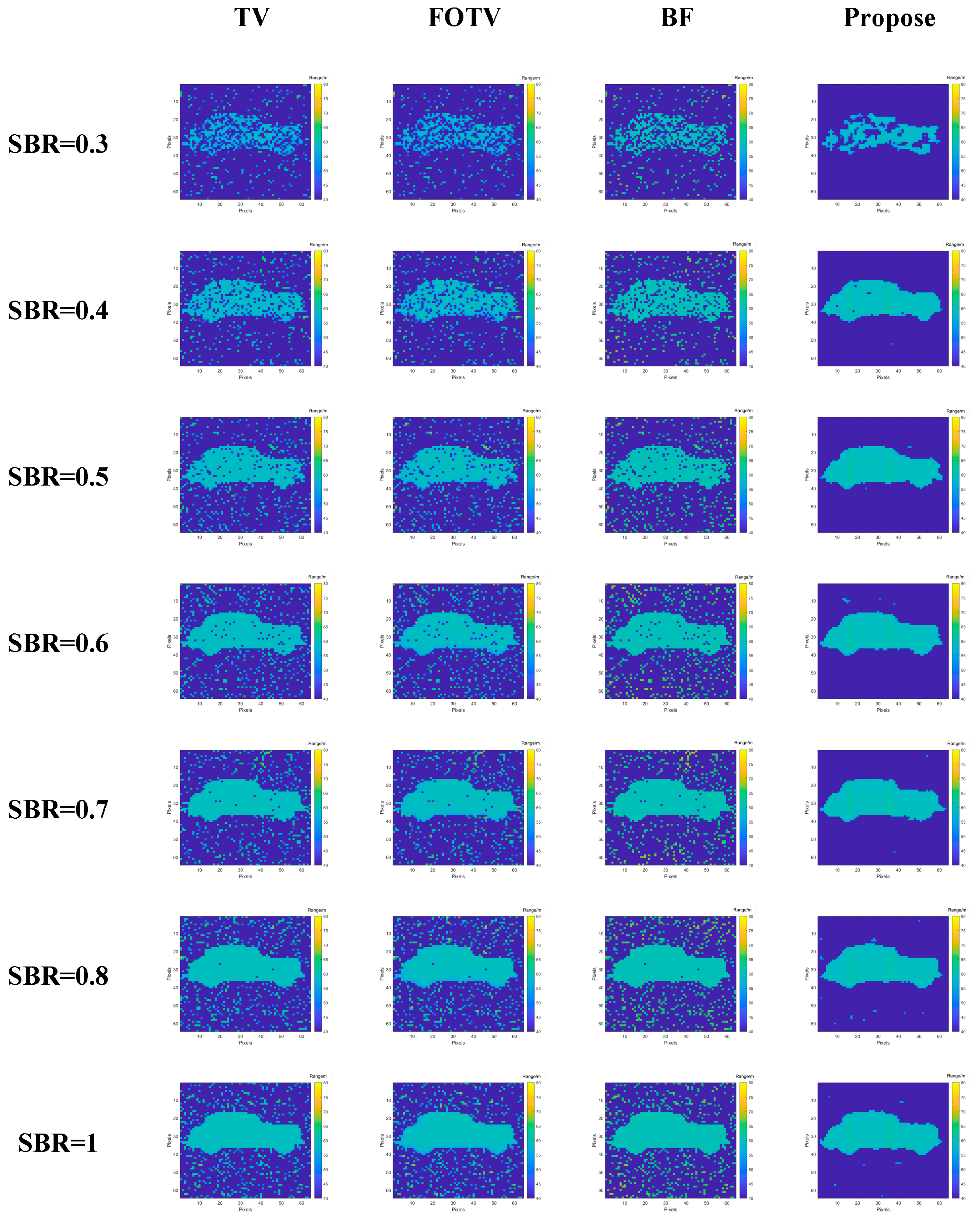
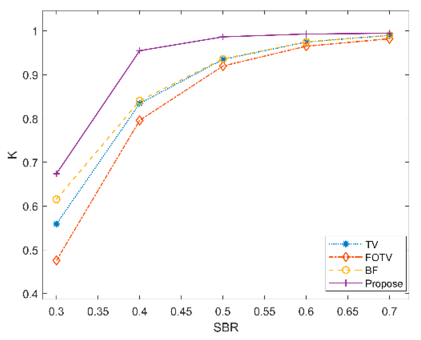
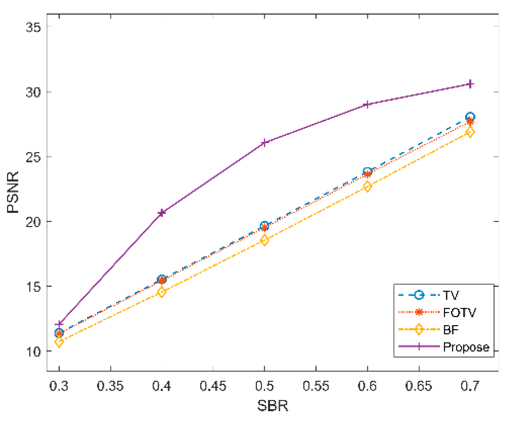
3.2.2. Simulation Analysis of Range Images with Different SBRs under 20 Frames

In order to verify the denoising performance of the algorithm proposed in this paper with the same frame number as that used in Section 3.2.1 but with different SBRs, the SBRs were set to 0.3, 0.4, 0.5, 0.6, and 0.7. The K and PSNR were used to assess the denoising performance. The single Monte Carlo simulation results of 20 frames with different SBRs are shown in Figure 4.

As can be seen in Figure 4, when the SBR is equal to 0.3, there is a large amount of noise at the target position in the range image when processed by the TV, FOTV, and BF algorithms, and the integrity and contour information of the target is poor. The algorithm proposed in this paper filters out most of the noise at the target position and can roughly identify the contour information of the target, but the interior of the target is incomplete. When the SBR is equal to 0.4, the range image processed by the TV, FOTV, and BF algorithms has a complete target that is roughly recovered, but there is still noise, and the smoothness of the range image is poor. This algorithm not only recovers the complete target precisely compared with the others but also shows few differences with the standard image and has a good denoising effect. When the SBR = 0.8, the range image target processed by the TV, FOTV, and BF algorithms is complete and smooth, but there is still a small amount of noise. This algorithm still ensures a good denoising effect.

In order to verify the stability of the denoising performance of the algorithm proposed with the same frame number and different SBRs, Monte Carlo experiments were conducted 1000 times on the TV, FOTV, and BF algorithms alongside the algorithm proposed in this paper. The K, PSNR, and SSIM were used to evaluate the range image processed by each algorithm. The average values of each index are shown in

Table 2. Denoising results of different signal-to-background ratios at frame 20.

SBRS	TV		FOTV		BF		Proposed
SBR = 0.3	K	0.5589	K	0.4757	K	0.6154	K	0.6738
	PSNR	11.3933	PSNR	11.3409	PSNR	10.7250	PSNR	12.0630
SBR = 0.4	K	0.8342	K	0.7958	K	0.8405	K	0.9549
	PSNR	15.5224	PSNR	15.4328	PSNR	14.5584	PSNR	20.6488
SBR = 0.5	K	0.9350	K	0.9199	K	0.9361	K	0.9865
	PSNR	19.6460	PSNR	19.5210	PSNR	18.5497	PSNR	26.0541
SBR = 0.6	K	0.9747	K	0.9651	K	0.9750	K	0.9929
	PSNR	23.8157	PSNR	23.6289	PSNR	22.6735	PSNR	29.0068
SBR = 0.7	K	0.9900	K	0.9822	K	0.9902	K	0.9947
	PSNR	28.0463	PSNR	27.6851	PSNR	26.8942	PSNR	30.5839

.

According to the above data, K and PSNR curves under different signal-to-background ratios under 20 frames are drawn, as shown in Figure 5.

As is discernible from Figure 5 and Figure 6, the increase in the SBR, K, and PSNR of each algorithm is improved to varying degrees, and the K and PSNR of the algorithm proposed are superior to those of the comparison algorithms in regard to the SBRs. When the SBR is 0.4, the K value of the TV, FOTV, and BF algorithms is less than 85%, and the PSNR is less than 16, while the target K value of the algorithm in this paper reaches 95.49%, and the PSNR value reaches 20.6488. It is proved that the algorithm proposed has good denoising performance. When the SBR is 0.5, the K value of the algorithm proposed reaches 0.9865, which is at least 5.11% higher than that of the other algorithms, and the PSNR value reaches 26.0541, which is at least 24.6% higher than that of the other algorithms.

The fractional-order derivative is a global operator with long memory, which distinguishes it from integer-order derivatives. When the depth image of a target contains a large amount of noise, establishing connections between pixels can increase the influence of noise on the current pixel. TV’s results are better than FOTV’s results.

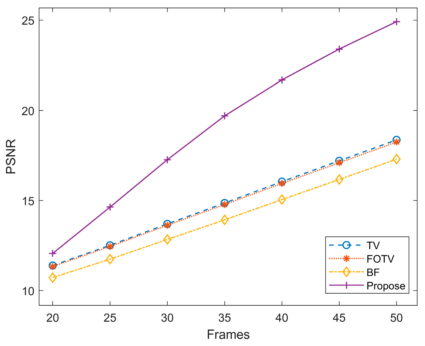
3.2.3. Simulation Analysis of Range Image with Different Frame Numbers When SBR Is 0.5

In order to verify the influence of different statistical frames on the denoising performance of the algorithm proposed, the simulation data from when the SBR = 0.5 were selected to discuss the processing results of the TV, FOTV, and BF algorithms and the algorithm proposed in this paper when the frame numbers were 20, 25, 30, 35, 40, 45, and 50. The single Monte Carlo simulation results when the SBR is equal to 0.5 with different frame numbers are shown in

Table 3. Denoising results of different frames when SBR = 0.5.

Frames	TV		FOTV		BF		Proposed
20	K	0.5589	K	0.4757	K	0.6154	K	0.6738
	PSNR	11.3933	PSNR	11.3409	PSNR	10.7250	PSNR	12.0630
25	K	0.6648	K	0.5867	K	0.6958	K	0.8198
	PSNR	12.5166	PSNR	12.4527	PSNR	11.7458	PSNR	14.6361
30	K	0.7469	K	0.6841	K	0.7634	K	0.9018
	PSNR	13.7025	PSNR	13.6282	PSNR	12.8409	PSNR	17.2648
35	K	0.8067	K	0.7586	K	0.8157	K	0.9439
	PSNR	14.8628	PSNR	14.7775	PSNR	13.9279	PSNR	19.6990
40	K	0.8525	K	0.8179	K	0.8576	K	0.9645
	PSNR	16.0490	PSNR	15.9514	PSNR	15.0531	PSNR	21.6841
45	K	0.8864	K	0.8600	K	0.8897	K	0.9760
	PSNR	17.2072	PSNR	17.1003	PSNR	16.1692	PSNR	23.3974
50	K	0.9126	K	0.8921	K	0.9148	K	0.9827
	PSNR	18.3680	PSNR	18.2520	PSNR	17.2977	PSNR	24.9162

.

From Figure 7 and Figure 8, it can be seen that the K and PSNRs of each algorithm are improved to varying degrees with the increase in the statistical frame number. When the statistical frame number was 25, the K of the TV, FOTV, and BF algorithms did not exceed 70%. In contrast, the K of the algorithm proposed reached 0.8198, which indicates a better denoising of the range image. When the quantity of image frames is 35, compared with the other comparison algorithms, the K and PSNR of the algorithm proposed are improved by at least 13.58% and 24.55%.

4. Experimental Verification

4.1. Experimental System Construction

A 64 × 64 array GM-APD was selected as the detector of the system when building the laser radar system with a separate transmitter and receiver, as shown in Figure 9. The transmit–receive field of view was $0.9°\times 0.9°$, and a 1064 nm fiber laser was selected as the laser source, of which the pulse laser output energy was set to 110 uJ with a 10 ns pulse width and 15 kHz repetition frequency.

4.2. Experimental Data Processing and Analysis

Imaging experiments were conducted on residential buildings with a range of 446.1 m to 463.2 m under strong sunlight to verify the denoising performance of the algorithm proposed. The scenario of the target area is shown in Figure 10. In order to obtain the ideal range image, the same target region was detected and imaged by the peak-picking method at night. A total of 5000 frames were used for the multi-frame statistics. The image obtained was taken as the ideal range image of the target, as shown in Figure 11.

In the daytime imaging experiment, the SBR was equal to 0.8. In the case of 100 frames, the TV denoising, FOTV denoising, and BF denoising algorithms, as well as the algorithm proposed in this paper, were used to denoise the range image obtained by the maximum likelihood estimation method. Figure 12, Figure 13, Figure 14 and Figure 15 show the result after denoising.

The denoising algorithm designed in this paper can denoise the target range image better than the contrast method and produce a smoother target region. Various indicators were used to evaluate the reconstructed range image quality, the data results are shown in

Table 4. Range image reconstruction results.

Evaluation Metric	TV Denoising	FOTV Denoising	BF Denoising	Proposed
K	0.8270	0.7828	0.8885	0.9283
PSNR	4.6869	4.6866	4.6871	4.6969

.

The denoising method proposed in this paper improves the target restoration degree by at least 4.29%, and the PSNR is 4.6969, both of which are better than those of the comparison algorithms. For GM-APD range images, the method provided in this paper’s denoising performance has been successfully verified as good.

In order to verify the advancement of our algorithm, our algorithm is compared with [21] in the case of 100 frames, and the SBR is 0.8. Figure 16 shows the denoised results. The comparative data between [21] and the algorithm proposed are presented in

Table 5. Range image reconstruction results.

Evaluation Metric	[21]	Proposed
K	0.8965	0.9283
PSNR	4.4421	4.6969

.

Both K and PSNR of the proposed algorithm are superior to the comparison algorithm, which can verify the advancement of the proposed algorithm.

5. Discussion

In order to achieve the denoising of GM-APD lidar range images with a low SBR, a fractional-order total variational GM-APD lidar range-image denoising method based on a spatial kernel function and range kernel function was proposed. The simulation results show that when the SBR is equal to 0.4, and the statistical frame number is 20, compared with BF denoising, FOTV denoising, and TV denoising, the K and PSNR of the algorithm proposed here are improved by at least 11.98% and 24.83%, respectively. The experimental results show that when the SBR is 0.8 and the statistical frame number is 100, the K of the algorithm proposed increases by at least 0.2% compared with that obtained via BF denoising, FOTV denoising, and TV denoising. It can be seen that the denoising method proposed in this paper has a good image denoising effect under the condition of a low SBR.

References

1. Shi, X.; Lu, W.; Sun, J.; Ge, W.; Zhang, H.; Li, S. Suppressing the influence of GM-APD coherent lidar saturation by signal modulation. Optik 2023, 275, 170619. [Google Scholar] [CrossRef]
2. Liu, D.; Sun, J.; Lu, W.; Li, S.; Zhou, X. 3D reconstruction of the dynamic scene with high-speed targets for GM-APD LiDAR. Opt. Laser Technol. 2023, 161, 109114. [Google Scholar] [CrossRef]
3. Wang, M.; Sun, J.; Li, S.; Lu, W.; Zhou, X.; Zhang, H. Research on infrared image guided GM-APD range image recovery algorithm under limited detections. Opt. Lasers Eng. 2023, 166, 107579. [Google Scholar] [CrossRef]
4. Huang, M.; Zhang, Z.; Cen, L.; Li, J.; Xie, J.; Zhao, Y. Prediction of the Number of Cumulative Pulses Based on the Photon Statistical Entropy Evaluation in Photon-Counting LiDAR. Entropy 2023, 25, 522. [Google Scholar] [CrossRef]
5. Zhang, Y.; Li, S.; Sun, J.; Zhang, X.; Zhou, X.; He, R.; Zhang, H. Three-dimensional imaging of ships in the foggy environment using a single-photon detector array. Optik 2023, 272, 170310. [Google Scholar] [CrossRef]
6. Ding, Y.; Qu, Y.; Sun, J.; Du, D.; Jiang, Y.; Zhang, H. Long-distance multi-vehicle detection at night based on Gm-APD lidar. Remote Sens. 2022, 14, 3553. [Google Scholar] [CrossRef]
7. Zhang, Y.; Li, S.; Sun, J.; Liu, D.; Zhang, X.; Yang, X.; Zhou, X. Dual-parameter estimation algorithm for Gm-APD lidar depth imaging through smoke. Measurement 2022, 196, 111269. [Google Scholar] [CrossRef]
8. Liu, D.; Sun, J.; Gao, S.; Ma, L.; Jiang, P.; Guo, S.; Zhou, X. Single-parameter estimation construction algorithm for Gm-APD lidar imaging through fog. Opt. Commun. 2021, 482, 126558. [Google Scholar] [CrossRef]
9. Jiang, Y. Adaptive Suppression Method of LiDAR Background Noise Based on Threshold Detection. Appl. Sci. 2023, 13, 3772. [Google Scholar] [CrossRef]
10. Green, T.J., Jr.; Shapiro, J.H. Detecting objects in three-dimensional laser radar range images. Opt. Eng. 1994, 33, 865–874. [Google Scholar] [CrossRef]
11. Saban, I.; Faibish, S. Image processing techniques for laser images. In Proceedings of the 1996 Canadian Conference on Electrical and Computer Engineering, Calgary, AB, Canada, 26–29 May 1996; Volume 1, pp. 462–465. [Google Scholar] [CrossRef]
12. Yu, J.; Yang, S.; Zhu, B. Noise suppression and the method evaluation for ladar range images. J. Optoelectron. Laser 2015, 26, 1215–1221. [Google Scholar] [CrossRef]
13. Wang, M.; Sun, J.; Li, S.; Lu, W.; Zhou, X.; Zhang, H. A photon-number-based systematic algorithm for range image recovery of GM-APD lidar under few-frames detection. Infrared Phys. Technol. 2022, 125, 104267. [Google Scholar] [CrossRef]
14. Xia, Z.W.; Li, Q.; Xiong, Z.P.; Wang, Q. Ladar range image denoising by a nonlocal probability statistics algorithm. Opt. Eng. 2013, 52, 017003. [Google Scholar] [CrossRef]
15. Halimi, A.; Altmann, Y.; McCarthy, A.; Ren, X.; Tobin, R.; Buller, G.S.; McLaughlin, S. Restoration of intensity and depth images constructed using sparse single-photon data. In Proceedings of the 24th European Signal Processing Conference (EUSIPCO), Budapest, Hungary, 29 August–2 September 2016; pp. 86–90. [Google Scholar] [CrossRef]
16. Chen, S.; Halimi, A.; Ren, X.; McCarthy, A.; Su, X.; McLaughlin, S.; Buller, G.S. Learning Non-Local Spatial Correlations To Restore Sparse 3D Single-Photon Data. IEEE Trans. Image Process. 2020, 29, 3119–3131. [Google Scholar] [CrossRef] [PubMed]
17. Wu, M.; Lu, Y.; Li, H.; Mao, T.; Guan, Y.; Zhang, L.; He, W.; Wu, P.; Chen, Q. Intensity-guided depth image estimation in long-range lidar. Opt. Lasers Eng. 2022, 155, 107054. [Google Scholar] [CrossRef]
18. Li, C.; He, C. Fractional-order diffusion coupled with integer-order diffusion for multiplicative noise removal. Comput. Math. Appl. 2023, 136, 34–43. [Google Scholar] [CrossRef]
19. Huang, T.; Wang, C.; Liu, X. Depth Image Denoising Algorithm Based on Fractional Calculus. Electronics 2022, 11, 1910. [Google Scholar] [CrossRef]
20. Wang, X.; Wang, C.; Xie, D.; Wei, X.; Huang, T.; Liu, X. A spatially correlated fractional integral-based method for denoising geiger-mode avalanche photodiode light detection and ranging depth images. Optik 2023, 288, 171244. [Google Scholar] [CrossRef]
21. Xie, D.; Wang, X.; Wang, C.; Yuan, K.; Wei, X.; Liu, X.; Huang, T. A Fractional-Order Total Variation Regularization-Based Method for Recovering Geiger-Mode Avalanche Photodiode Light Detection and Ranging Depth Images. Fractal Fract. 2023, 7, 445. [Google Scholar] [CrossRef]
22. Wang, F.; Zhao, Y.; Zhang, Y.; Sun, X. Range accuracy limitation of pulse ranging systems based on Geiger mode single-photon detectors. Appl. Opt. 2010, 49, 5561–5566. [Google Scholar] [CrossRef]
23. Chen, D.; Chen, Y.; Xue, D. Fractional-order total variation image denoising based on proximity algorithm. Appl. Math. Comput. 2015, 257, 537–545. [Google Scholar] [CrossRef]
24. Zhou, Y.; Li, Y.; Guo, Z.; Wu, B.; Zhang, D. Multiplicative Noise Removal and Contrast Enhancement for SAR Images Based on a Total Fractional-Order Variation Model. Fractal Fract. 2023, 7, 329. [Google Scholar] [CrossRef]
25. Parvaz, R. Image restoration with impulse noise based on fractional-order total variation and framelet transform. SIViP 2023, 17, 2455–2463. [Google Scholar] [CrossRef]
26. Tom, G.; Stanley, O. The split Bregman method for L1-regularized problems. SIAM J. Imaging Sci. 2009, 2, 323–343. [Google Scholar] [CrossRef]
27. Micchelli, C.; Shen, L.; Xu, Y. Proximity algorithms for image models: Denoising. Inverse Probl. 2011, 27, 045009. [Google Scholar] [CrossRef]
28. Zhao, M.; Wang, Q.; Ning, J. A region fusion based split Bregman method for TV denoising algorithm. Multimed. Tools Appl. 2021, 80, 15875–15900. [Google Scholar] [CrossRef]
29. Cheng, S.W.; Lin, Y.T.; Peng, Y.T. A Fast Two-Stage Bilateral Filter Using Constant Time O(1) Histogram Generation. Sensors 2022, 22, 926. [Google Scholar] [CrossRef]
30. Ma, L.; Sun, J.; Jiang, P.; Liu, D.; Zhou, X.; Wang, Q. Signal extraction algorithm of Gm-APD lidar with low SNR return. Optik 2020, 206, 164340. [Google Scholar] [CrossRef]
31. Berginc, G.; Jouffroy, M. Simulation of 3D laser imaging. PIERS Online 2010, 6, 415–419. [Google Scholar] [CrossRef]
Figure 1. Algorithm principle diagram.
Fractalfract 07 00674 g001
Figure 2. Fractional differential magnitude–frequency response.
Fractalfract 07 00674 g002
Figure 3. Simulated vehicle range image.
Fractalfract 07 00674 g003
Figure 4. Denoising results of different signal-to-background ratio range images in 20 frames.
Fractalfract 07 00674 g004
Figure 5. K of different SBRs when the number of frames is 20.
Fractalfract 07 00674 g005
Figure 6. PSNR of different SBRs when the number of frames is 20.
Fractalfract 07 00674 g006
Figure 7. K of different frames when SBR = 0.5.
Fractalfract 07 00674 g007
Figure 8. PSNR of different frames when SBR = 0.5.
Fractalfract 07 00674 g008
Figure 9. System diagram.
Fractalfract 07 00674 g009
Figure 10. Target scene.
Fractalfract 07 00674 g010
Figure 11. Ideal target range image.
Fractalfract 07 00674 g011
Figure 12. TV.
Fractalfract 07 00674 g012
Figure 13. FOTV.
Fractalfract 07 00674 g013
Figure 14. BF.
Fractalfract 07 00674 g014
Figure 15. Proposed algorithm.
Fractalfract 07 00674 g015
Figure 16. Algorithm [21].
Fractalfract 07 00674 g016