Article

A New Hybrid Optimal Auxiliary Function Method for Approximate Solutions of Non-Linear Fractional Partial Differential Equations

1
Department of Mathematics, Abdul Wali Khan University Mardan, Mardan 23200, Pakistan
2
Department of Mathematics, University of South Australia, Adelaide, SA 5000, Australia
3
Department of Mathematics, College of Education for Pure Sciences, University of Anbar, Ramadi 31001, Iraq
4
Department of Mathematics, College of Education for Pure Sciences, University of Basrah, Basrah 61001, Iraq
5
Institute of Mathematics, University of Debrecen, Pf. 400, H-4002 Debrecen, Hungary
6
College of Engineering Technology, National University of Science and Technology, Nasiriyah 64001, Iraq
7
Department of Mathematics, College of Sciences, University of Sharjah, Sharjah 27272, United Arab Emirates
8
Department of Mathematics and Computer Science, University of Oradea, 1 Universitatii Street, 410087 Oradea, Romania
*
Author to whom correspondence should be addressed.
Fractal Fract. 2023, 7(9), 673; https://doi.org/10.3390/fractalfract7090673
Submission received: 28 July 2023 / Revised: 28 August 2023 / Accepted: 31 August 2023 / Published: 7 September 2023
(This article belongs to the Section General Mathematics, Analysis)

Abstract

:
This study uses the optimal auxiliary function method to approximate solutions for fractional-order non-linear partial differential equations, utilizing Riemann–Liouville’s fractional integral and the Caputo derivative. This approach eliminates the need for assumptions about parameter magnitudes, offering a significant advantage. We validate our approach using the time-fractional Cahn–Hilliard, fractional Burgers–Poisson, and Benjamin–Bona–Mahony–Burger equations. Comparative testing shows that our method outperforms new iterative, homotopy perturbation, homotopy analysis, and residual power series methods. These examples highlight our method’s effectiveness in obtaining precise solutions for non-linear fractional differential equations, showcasing its superiority in accuracy and consistency. We underscore its potential for revealing elusive exact solutions by demonstrating success across various examples. Our methodology advances fractional differential equation research and equips practitioners with a tool for solving non-linear equations. A key feature is its ability to avoid parameter assumptions, enhancing its applicability to a broader range of problems and expanding the scope of problems addressable using fractional calculus techniques.

1. Introduction

Many challenges that emerge in natural phenomena, including fluid mechanics, biology, and thermodynamics, can be effectively represented through mathematical models. These models can be translated into a mathematical framework using differential equations. Classifying these differential equations as either linear or non-linear is contingent upon the specific characteristics of the issues that manifest across various scientific domains. In contemporary times, a significant research thrust has been directed towards fractional-order differential equations. Fractional calculus stands as a refined adaptation of classical calculus. Addressing the challenge of solving non-linear fractional-order partial differential equations (FPDE) entails the utilization of a diverse array of both numerical and analytical methods.
Some non-linear fractional partial differential equations exist among these PDEs, such as time-fractional Cahn–Hilliard (TFCH) equations, fractional Burgers–Poisson equations, and BBM Burger equations. The Cahn–Hillard equation was named after Cahn and Hilliard in 1958 [1]. This equation is critical in order to comprehend a variety of interesting physical phenomena, such as spinodal decomposition, phase ordering dynamics, and phase separation processes. It also explains a critical qualitative distinguishing feature of two-phase systems (see [1,2,3,4] for a detailed discussion); furthermore, long memory processes and fractional integration in econometrics [5] and kinetics of phase decomposition processes [6] have also been discussed. Researchers have investigated mathematical and numerical solutions of TFCH equations [7,8,9,10,11] since the appearances of their real-life applications in the abovementioned fields. The fractional Burgers–Poisson (FBP) equation was proposed for the first time in 2004 to describe the propagation of long waves in dispersive media in a single direction [12]. The FBP equation models a unidirectional water wave with weaker dispersive effects than the KdV equation in shallow water. The BBM–Burger equation defines the mathematical model of the propagation of small-amplitude long waves in non-linear dispersive media.
The BBM equation is a refinement of the KdV equation, as is well known. The wave-breaking models are affected by the BBM–Burger equation and the KdV equation [13]. Water waves inspired the KdV equation, which was later used as a basis for long waves in a variety of other physical systems. However, the KdV equation was not valid in certain long-wave physical systems. As a result, the BBM–Burger model was proposed, representing unidirectional long-wave propagation in a non-linear dispersive system [13,14,15]. Solving fractional differential equations and fractional partial differential equations has been a significant focus for researchers. Since most fractional differential equations do not have exact analytic solutions, approximate and numerical methods are commonly used [16,17,18], Baleanu et al. discussed the planar system-masses in an equilateral triangle [19], Ghanim et al. discussed certain implementations in fractional calculus operators, some new extensions on fractional differential and integral properties, and some analytical merits of the Kummer-type function [20,21,22], Almalahi et al. discussed qualitative analysis of the Langevin integro-fractional differential equation [23], Jajarmi et al. and Sajjadi et al. discussed a new iterative method for the numerical solution of high-order non-linear fractional boundary value problems and fractional optimal control problems with a general derivative operator [24,25,26], and Mohammadi et al. discussed a hybrid functions numerical scheme for fractional optimal control problems [27]. On the well-posedness of the sub-diffusion equation with the conformable derivative model, mathematical modeling for the adsorption process of the dye removal Laplace–Carson integral transformation for exact solutions [28,29,30,31] has been discussed in the literature in order to find the numerical and approximate solutions. Many analytical methods have been attempted in order to solve non-linear problems, including the new iterative method (NIM), homotopy perturbation method (HPM), homotopy analysis method (q-HAM), residual power series method (RPSM), and FHATM.
Similarly, using Riemann–Liouville’s (R-L) fractional integral and the Caputo derivative, we present another approach known as the optimal auxiliary function method (OAFM) for higher dimensional equations, which was first introduced by Vasile Marinca and colleagues for thin film flow problem [32]. Laiq Zada et al. later expanded the approach to partial differential and generalized seventh-order KDV equations [33]. Several other approaches and models have been developed recently to deal with different types of fractional-order equations and PDEs in general; see [34,35,36,37]. Auxiliary convergence control parameters and auxiliary functions are included in this approach to control and accelerate the method’s convergence. The OAFM operates without the need for presuming any parameter to be small or large. This proposed technique possesses the benefit of adeptly handling both linear and non-linear challenges while preserving a broad scope of applicability and effectiveness. The rest of this work is structured as follows. We begin with an initial section that provides essential definitions aimed at aiding the readers’ comprehension. Following this, the subsequent section outlines the fundamental concepts underlying the OAFM. Moving forward, in the third section, we apply the OAFM to tackle fractional-order problems, leading to the derivation of valuable solutions that are accurately presented through tables and graphs. Exploring deeper, the fourth and fifth sections provide a comprehensive analysis and discussion of the presented tables and graphs, respectively. Finally, we conclude our study in the sixth section, summarizing the key findings and suggestions drawn from our work.

2. Preliminaries

We need some basic definitions to investigate our problems with the help of OAFM.
Definition 1 
([38]). Riemann–Liouville fractional integral left-sided:
I R L a + α f r = 1 Γ α a η η r α 1 f r d r η a ,
Definition 2 
([38]). Riemann–Liouville right-sided integral:
I R L b α f η = 1 Γ α η b r η α 1 f r d r η b ,
Definition 3 
([38]). Modified Riemann–Liouville fractional derivative:
D f r = 1 Γ 1 α d d η 0 η η r α [ f r f 0 ] d r .
Definition 4 
([38]). Liouville derivative:
D α f ( η ) = 1 Γ 1 α d d η η η r α f r d r , η
Definition 5 
([38]). Liouville left-sided derivative:
D 0 + α f ( η ) = 1 Γ η α d n d η n 0 η η r α + n + 1 f r d r , η 0 .
Definition 6 
([38]). Liouville right-sided derivative:
D α f ( η ) = 1 n Γ η α d n d η n η η r α + n 1 f r d r , η .
Definition 7 
([38]). Right Riemann–Liouville integral of variable fractional order:
I η b α f r = η b η r α r , η 1 f r d r Γ α r , η .

3. The Basic Idea of the Optimal Auxiliary Function Method

In this paper, we successfully applied the OAFM to solve the analytical approximate non-linear fractional solution of partial differential equations. We consider the most general form of a non-linear differential equation.
The following are the general PDEs:
α θ ( η , r ) r α = ( η , r ) + N θ ( η , r ) = 0 ,
They are subject to boundary conditions:
α k r θ ( η , r ) = h k ( η ) . ( k = 0 , 1 , , n 1 ) α n r θ ( η , 0 ) = 0 , n = [ α ] . k r θ ( η , 0 ) = g k ( η ) . ( k = 0 , 1 , , n 1 ) n r θ ( η , 0 ) = 0 , n = [ α ] .
In Equation (8), α r α shows the Caputo or R-L operator θ ( η , r ) unknown function while ( η , r ) is a known analytic function.
Step 1: To find the approximate solution of Equation (9), we have to consider the approximate solution in the form of two components shown in Equation (10).
θ ^ ( η , r ) = θ 0 ( η , r ) + θ 1 ( η , r , c ι ) , ι = 1 , 2 , 3 , 4 , 5 δ .
Step 2: We arrange an equation to find the zero- and first-order solution (10) into Equation (8). Its results are
α θ 0 ( η , r ) r α + α θ 1 ( η , r ) r α + ( η , r ) + Ν α θ 0 ( η , r ) r α + α θ 1 ( η , r ) , C i r α = 0 .
Step 3: The initial approximation θ 0 ( η , r ) can be obtained from the linear equation as
α θ 0 ( η , r ) r α + ( η , r ) = 0 ,
Applying the inverse operator, we obtain θ 0 ( η , r ) as follows:
θ 0 ( η , r ) = η , r
Step 4: Expand the non-linear term from Equation (11) in the form of
Ν α θ 0 ( η , r ) r α + α θ 1 ( η , r , C i ) r α = Ν θ 0 ( η , r ) + k = 1 θ 1 k k ! Ν ( k ) θ 0 ( η , r ) .
Step 5: To solve Equation (14) easily and accelerate the convergence of the first-order approximation, we introduce another expression that can be written as follows:
α θ 1 ( η , r , C i ) r α = E 1 θ 0 ( η , r ) Ν θ 0 ( η , r ) E 2 θ 0 ( η , r ) , C j ,
Remark 1. 
Where  E 1  and  E 2  are two auxiliary functions depending upon  θ 0 ( η , r )  and the convergence control parameter  C ι  and  C J , ι = 1 , 2 , 3 , 4 , J = s + 1 , s + 2 , δ .
Remark 2. 
E 1  and  E 2  are of the form  θ 0 ( η , r ) , N θ 0 ( η , r ) , or the combination of both  θ 0 ( η , r ) ,  and  N θ 0 ( η , r ) , but they are not unique.
Remark 3. 
If  θ 0 ( η , r ) ,  or  N θ 0 ( η , r )  are the functions of a polynomial, then  E 1 θ 0 ( η , r ) , C ι  and  E 2 θ 0 ( η , r ) , C j  are taken as the summation. If  θ 0 ( η , r ) ,  or  N θ 0 ( η , r )  are the exponential functions, then  E 1 θ 0 ( η , r ) , C ι  and  E 2 θ 0 ( η , r ) , C j  are taken as the functions of addition of an exponential function. If  θ 0 ( η , r ) ,  or  N θ 0 ( η , r )  are in the form of a trigonometric function, then  E 1 θ 0 ( η , r ) , C ι  and  E 2 θ 0 ( η , r ) , C j  are taken as the addition of a trigonometric function. A special case for If  N θ 0 ( η , r ) = 0  then  θ 0 ( η , r ) ,  is the exact solution of Equation (10).
Step 6: To find the square of the residual error to obtain the values of C ι and C j we use either the collocation method, the Galerkin method, the Ritz method, or the least square method.
H C ι , C j = 0 r Ω R 2 η , r ; C ι , C j d η d r ,
where R is the residual,
R η , r , C i , C j = α θ ^ ( η , r ) , C i , C J r + ( η , r ) + Ν θ ^ η , r , C i , C j , i = 1 , 2 , 3 s , j = s + 1 , s + 2 , s + 3 ρ , J C 1 = J C 2 = J C q = 0 .
In solving the above equations simultaneously, we obtain the values of the constants C ι .
Remark 4. 
This powerful tool does not depend on small or large parameters. Our procedure consists of auxiliary functions  E 1  and  E 2  which control the convergence of the approximate solution after only one iteration.

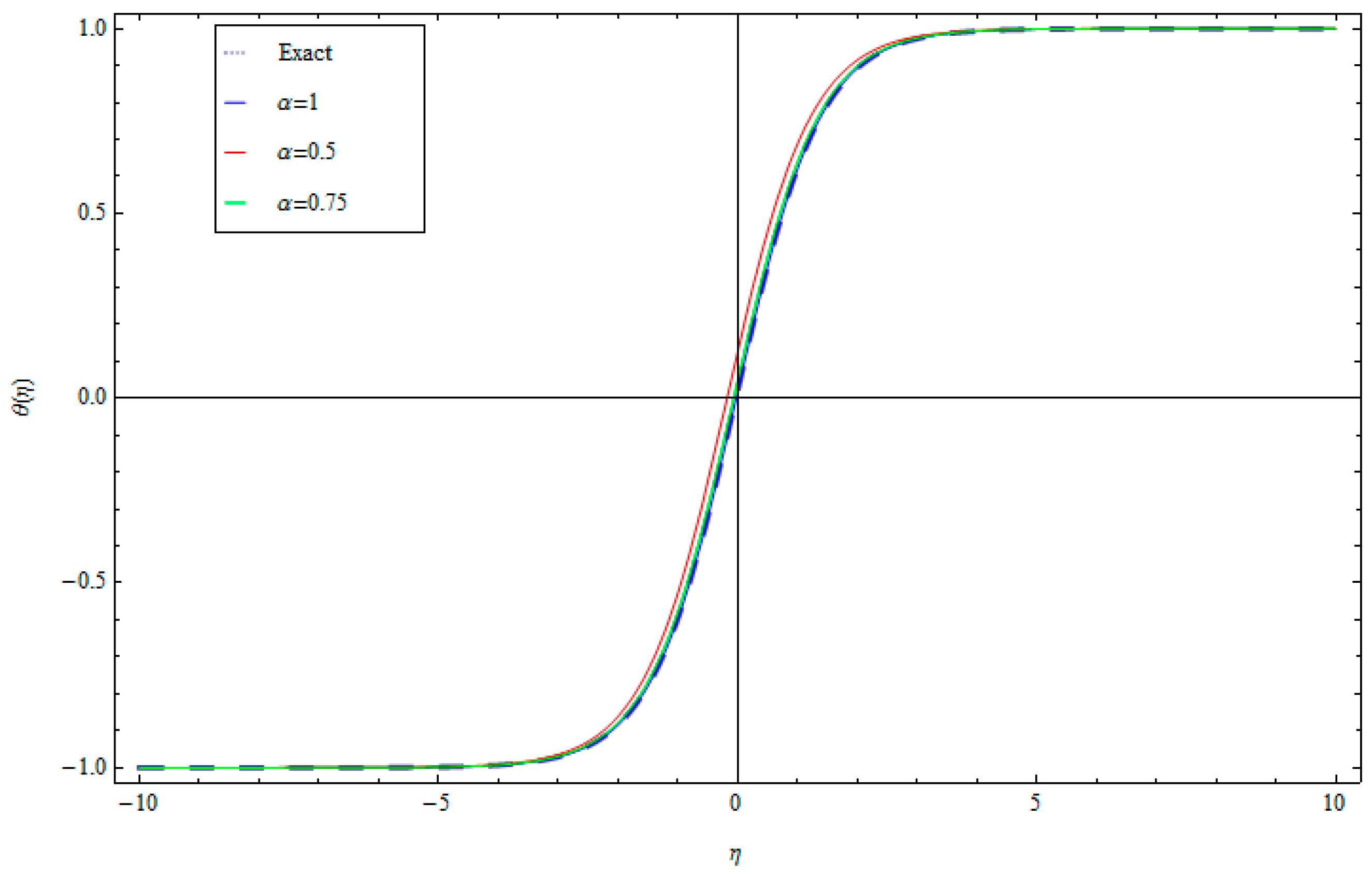
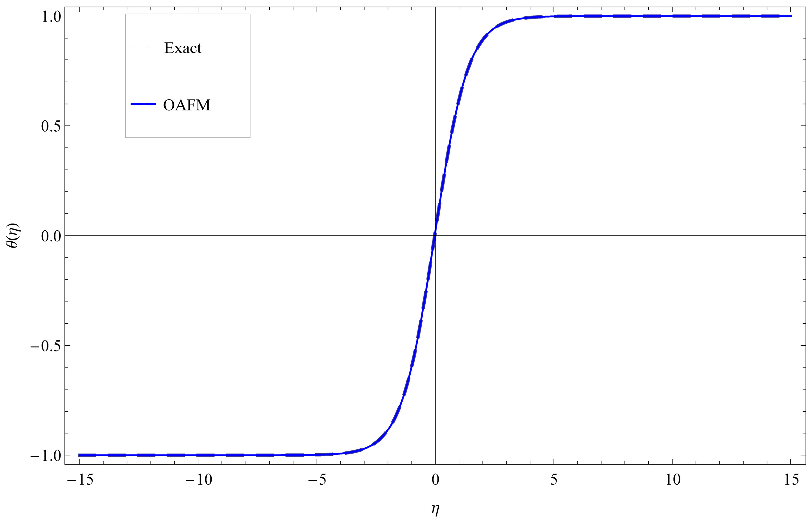
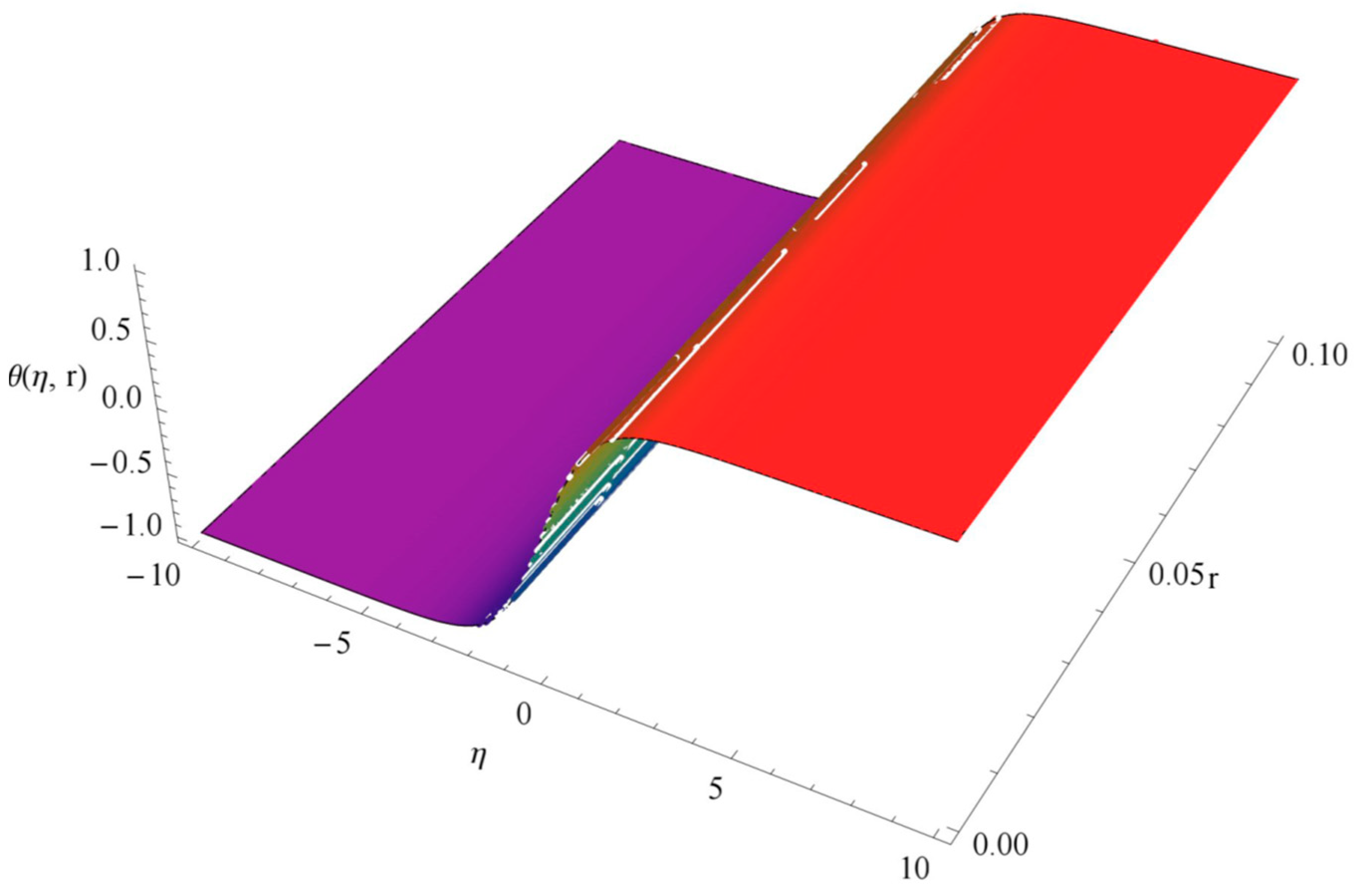
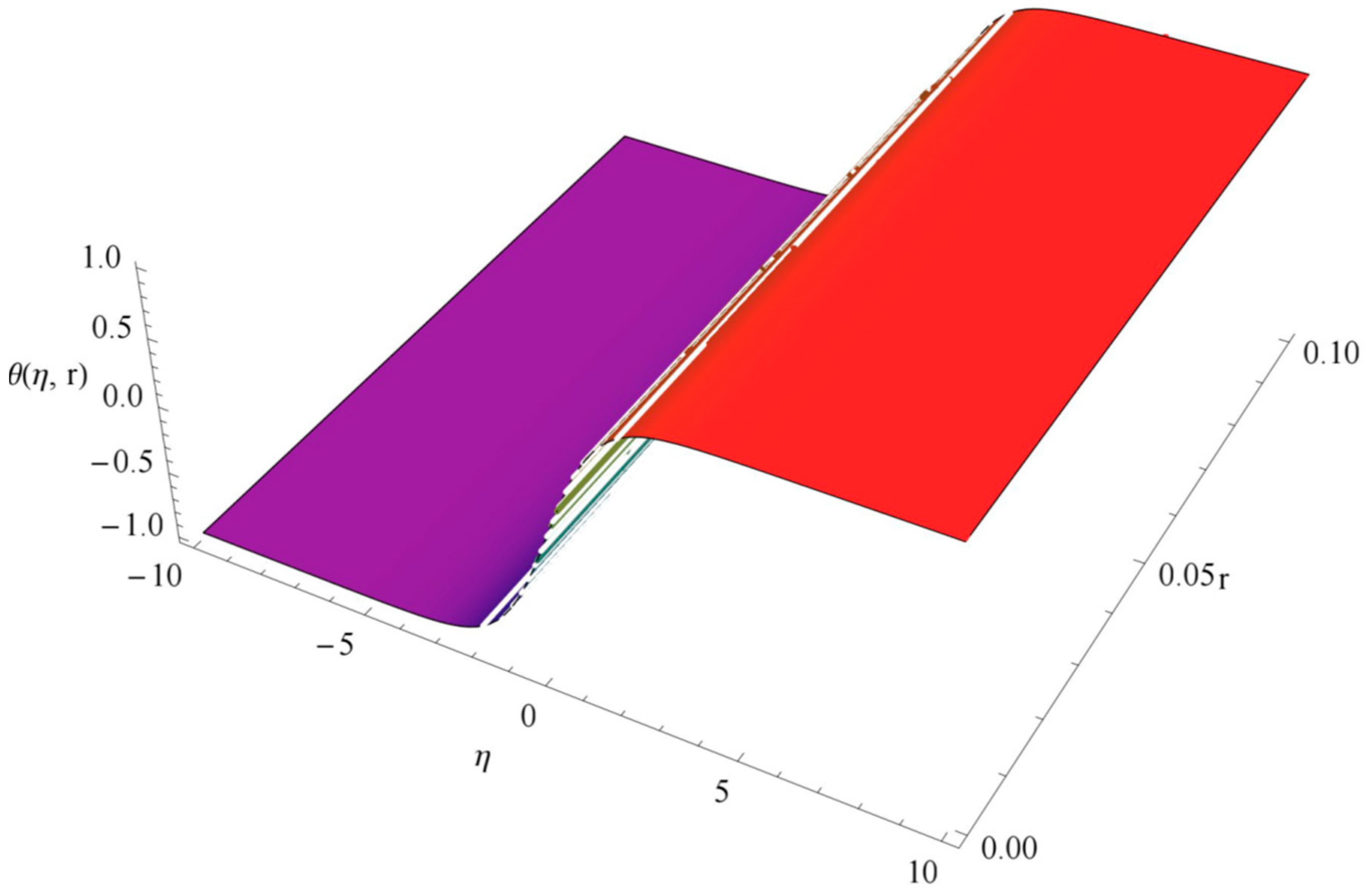
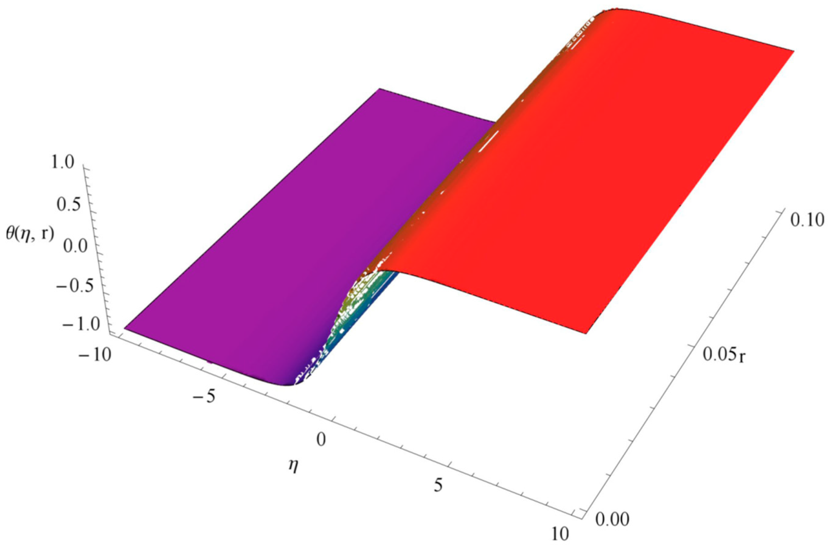
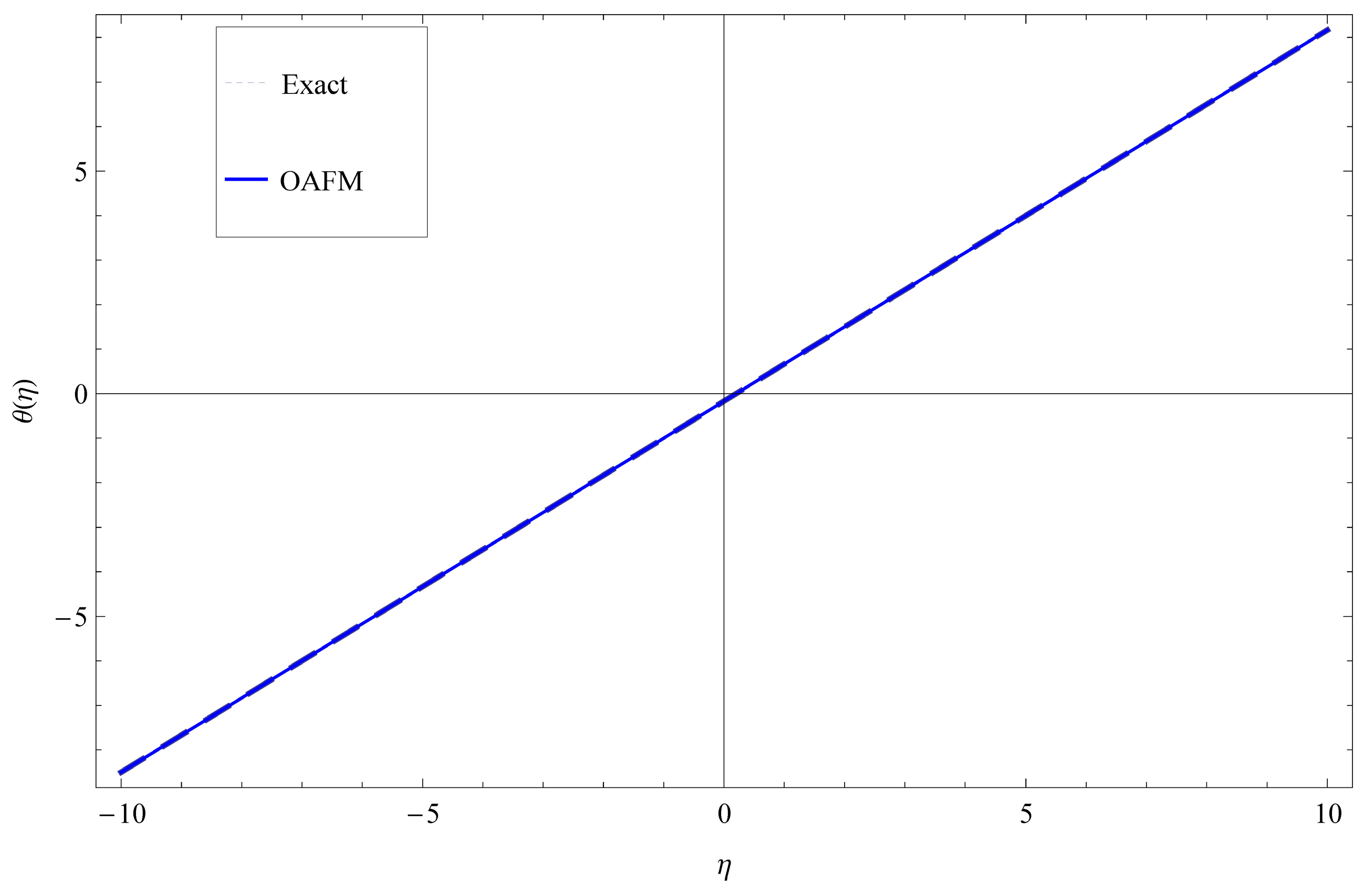
4. Numerical Experiments and Results

In this section, we present three problems and demonstrate how their numerical results compare with other methods from the literature.
Problem 1. 
Consider the time-fractional equation of Cahn–Hilliard [39]:
α θ ( η , r ) r α = μ θ ( η , r ) η + 6 θ ( η , r ) θ 2 ( η , r ) η + 3 θ 2 ( η , r ) 2 θ ( η , r ) η 2 2 θ ( η , r ) η 2 4 θ ( η , r ) η 4 , 0 < α 1 ,
Then, it is subject to the initial condition:
θ 0 η , 0 = tanh η 2
The exact solution of Equation (18) when α, µ = 1 is
θ ( η , r ) = tanh η + r 2
So, Equation (18) can be written as
α θ ( η , r ) r α μ θ ( η , r ) η 6 θ ( η , r ) θ 2 ( η , r ) η 3 θ 2 ( η , r ) 2 θ ( η , r ) η 2 + 2 θ ( η , r ) η 2 + 4 θ ( η , r ) η 4 = 0 .
In Equation (21), we take the linear and non-linear parts as
L θ ( η , r ) = α θ ( η , r ) r α N θ ( η , r ) = μ θ ( η , r ) η 6 θ ( η , r ) θ 2 ( η , r ) η 3 θ 2 ( η , r ) 2 θ ( η , r ) η 2 + 2 θ ( η , r ) η 2 + 4 θ ( η , r ) η 4 .
The initial approximation θ 0 ( η , r ) is obtained from Equation (12):
α θ ( η , r ) r α = 0 ,
In applying the inverse operator as mentioned in Equation (13), we obtain the following solution,
θ 0 η , r = tanh η 2
By using Equation (24) in Equation (22), the non-linear operator becomes
N θ 0 ( η , r ) = μ θ 0 ( η , r ) η 6 θ 0 ( η , r ) θ 0 2 ( η , r ) η 3 θ 0 2 ( η , r ) 2 θ 0 ( η , r ) η 2 + 2 θ 0 ( η , r ) η 2 + 4 θ 0 ( η , r ) η 4 .
The first approximation is given by (15):
α θ 1 ( η , r , C i ) r α = E 1 θ 0 ( η , r ) Ν θ 0 ( η , r ) E 2 θ 0 ( η , r ) , C j ,
Here, we select E 1 and E 2 according to the non-linear operator,
E 1 = { C 1 1 2 tanh 2 η 2 2 + C 1 1 2 tanh η 2 + tanh 3 η 2 r + C 1 1 12 2 + 4 2 tanh 2 η 2 3 2 tanh 4 η 2 r 2 + C 1 1 12 2 tanh η 2 5 tanh 3 η 2 + 3 tanh 5 η 2 r 3 + C 1 1 120 2 2 17 2 tanh 2 η 2 + 30 2 tanh 4 η 2 15 2 tanh 6 η 2 r 4 } E 2 = 0
Using Equations (24) and (25) in Equation (26), and apply the inverse operator, we obtain the first approximation as
θ 1 η , r = 1 120 α Γ α C 1 r α S e c h 2 η 2 2 2 30 5 r 2 + r 4 + 20 r 3 + r 2 tanh η 2 15 2 r 2 2 + r 2 tanh 2 η 2 30 r 3 tanh 3 η 2 + 15 2 r 4 tanh 4 η 2
in adding Equations (24) and (28), we obtain first-order approximate solutions as
θ ^ ( η , r ) = θ 0 ( η , r ) + θ 0 ( η , r , C 1 ) . θ ^ ( η , r ) = tanh η 2 + 1 120 α Γ α C 1 r α S e c h 2 η 2 2 2 30 5 r 2 + r 4 + 20 r 3 + r 2 tanh η 2 15 2 r 2 2 + r 2 tanh 2 η 2 30 r 3 tanh 3 η 2 + 15 2 r 4 tanh 4 η 2
Below, the results of Problem 1 are presented in Table 1 and Table 2 and visualized in Figure 1, Figure 2, Figure 3, Figure 4, Figure 5 and Figure 6.
Problem 2. 
Consider the fractional Burgers–Poisson Equation [40]:
α θ ( η , r ) r α α r α 2 θ ( η , r ) η 2 + θ ( η , r ) η + θ ( η , r ) θ ( η , r ) η 3 θ ( η , r ) η 2 θ ( η , r ) η 2 + θ ( η , r ) 3 θ ( η , r ) η 3 = 0 , r > 0 , 0 < α 1 .
Then, it is subject to the initial condition:
θ 0 η , 0 = η
The exact solution of Equation (30) at α = 1 is
θ η , r = 1 + η 1 + r 1
According to the non-linear operator, we choose E 1 and E 2 for problem 2.
E 1 = C 1 + 3 C 2 r + 2 C 3 r 2 + 2 C 4 r 3 + 2 C 5 r 4 E 2 = 0
Using the same procedure of the OAFM method, we obtain the zero-order and first-order solution as
θ 0 η , r = η ,
θ 1 η , r = r α C 1 + r 3 C 2 + 2 r C 3 + r C 4 + C 5 r 1 + η α Γ α ,
In combining Equations (34) and (35), we obtain the OAFM solution given by the following expression:
θ ^ ( η , r ) = θ 0 η , r + θ 1 ( η , r , C 1 , C 2 , C 3 , C 4 , C 5 , C 6 ) . θ ^ ( η , r ) = η + r α C 1 + r 3 C 2 + 2 r C 3 + r C 4 + C 5 r 1 + η α Γ α .
Below, the results of Problem 2 are presented in Table 3 and Table 4 and visualized in Figure 7, Figure 8, Figure 9 and Figure 10.
Problem 3. 
The BBM–Burger equation can be written as [41]
α θ ( η , r ) r α 3 θ ( η , r ) η 2 r + θ ( η , r ) η + θ 2 ( η , r ) 2 η = 0 , r > 0 , η I R , α 0 , 1 ,
with the initial conditions of
θ 0 η , 0 = S e c h 2 η 4 .
The exact solution of Equation (37) at α = 1 is:
θ ( η , r ) = sec h 2 η 4 r 4 .
According to the non-linear operator, we choose E 1 and E 2 for problem number 3:
E 1 = C 1 1 2 S e c h 2 η 4 tanh η 4 E 2 = 0 ,
Using the same procedure of the OAFM method, we obtain the zero-order and first-order solution as
θ 0 ( η , r ) = S e c h 2 η 4 .
θ 1 η , r , C 1 = C 1 r α S e c h 2 η 4 tanh η 4 2 α Γ α
We obtain the first-order approximate solution by combining Equations (41) and (42).
θ ^ ( η , r ) = θ 0 ( η , r ) + θ 1 ( η , r , C 1 ) , θ ^ ( η , r ) = S e c h 2 η 4 + C 1 r α S e c h 2 η 4 tanh η 4 2 α Γ α .
Below, the results of Problem 3 are presented in Table 5 and Table 6 and visualized in Figure 11, Figure 12, Figure 13, Figure 14, Figure 15, Figure 16, Figure 17 and Figure 18.

5. Discussion

This section discusses the results of the optimal auxiliary function method (OAFM) for solving fractional-order equations. In this study, Mathematica 9 was employed for all of our computational work. The accuracy and the validity of the method were evaluated by comparing the results obtained with other analytical methods available in the literature. Table 1 show the numerical values of convergence control parameters obtained using the collocation technique. Table 2 represents the absolute error of the OAFM, comparing it with NIM and q-HAM using the exact solution α = μ = 1 . Table 3 shows the numerical values of convergence control parameters obtained using the Galerkin method (for the fractional Burgers-Poisson equation, we used the Galerkin method because, for this problem, the collocation method did not provide us with a rapid result).
Similarly, Table 4 compares OAFM results with exact and HPM solutions; the absolute error shows that our method is more accurate than the HPM. These tables demonstrate the accuracy of the OAFM by evaluating the absolute errors for different problems with their exact solutions. Table 5 and Table 6 present a comparative analysis of OAFM solutions with RPSM solutions and exact solutions for various α values, along with a comparison of absolute errors in RPSM at α = 1 , respectively. These comparisons further validate the effectiveness of the OAFM in delivering precise solutions.
Visual representations are provided through 2D and 3D graphs to complement the numerical results. Figure 1 and Figure 2 display 2D graphs for problem 1 with varying values of α , while Figure 3, Figure 4, Figure 5 and Figure 6 show 3D graphs for problem 1. Additionally, Figure 7 and Figure 8 show 2D graphs for different values of α at r = 0.2 for problem 2, and Figure 9 and Figure 10 display 3D plots comparing the exact and OAFM solutions for problem 2. Furthermore, Figure 11, Figure 12, Figure 13, Figure 14, Figure 15 and Figure 16 show 3D graphs for problem 3 with different values of α , while Figure 17 and Figure 18 show 2D plots for varying α at r = 0.01 for problem 3.
Overall, the results presented in Table 2, Table 4, Table 5 and Table 6 indicate that, as the value of α approaches 1, the OAFM solution rapidly converges to the exact solution. Based on the presented results, we can confidently say that the OAFM approach delivers remarkably precise solutions.

6. Conclusions

The optimal auxiliary function method (OAFM) is a strong and reliable analytical tool, providing solutions that closely match the exact solutions for various fractional-order equations. The time-fractional Cahn–Hilliard equation, fractional Burgers–Poisson equation, and Benjamin–Bona–Mahony–Burger equations have all been successfully used for finding the approximate solutions by using the OAFM. We can conclude from the numerical results and the presented figures that the proposed method for fractional-order non-linear partial differential equations is very reliable and easy to use. In comparison to NIM, FHATM, q-HAM, RPSM, and HPM, the OAFM approach solutions converge quickly to the exact solution. Based on the mathematical findings, we determined that the proposed method is simple, quick, and effective.

Author Contributions

Conceptualization, R.A., R.N., O.A. and N.F.-Y.; methodology, A.H.A. and F.G.; software, A.H.A.; validation, A.A.L. and F.G.; formal analysis, R.A., R.N., O.A. and N.F.-Y.; investigation, R.A., R.N., O.A. and N.F.-Y.; resources, A.H.A.; data curation, A.H.A. and F.G.; writing—original draft preparation A.H.A.; writing—review and editing, A.A.L. and F.G.; visualization, A.H.A., A.A.L. and F.G.; supervision, F.G.; project administration, A.H.A.; funding acquisition, A.A.L. All authors have read and agreed to the published version of the manuscript.

Funding

The publication of this research was supported by the University of Oradea.

Data Availability Statement

Not applicable.

Conflicts of Interest

The authors declare no conflict of interest.

References

  1. Cahn, J.W.; Hilliard, J.E. Free Energy of a Non-Uniform System I: Interfacial Free Energy. J. Chem. Phys. 1958, 28, 258–267. [Google Scholar] [CrossRef]
  2. Cahn, J.W. On Spinodal Decomposition. Acta Metall. 1961, 9, 795–801. [Google Scholar] [CrossRef]
  3. Elliott, C.M. The Cahn-Hilliard Model for the Kinetics of Phase Separation, in Mathematical Models for Phase Change Problems; Rodrigues, J.F., Ed.; International Series of Numerical Mathematics; Birkhauser: Basel, Switzerland, 1989; Volume 88. [Google Scholar]
  4. Novick-Cohen, A. The Cahn-Hilliard Equation. In Handbook of Differential Equations, Evolutionary Partial Differential Equations; Dafermos, C.M., Pokorny, M., Eds.; Elsevier: Amsterdam, The Netherlands, 2008; Volume 4, pp. 201–228. [Google Scholar]
  5. Baillie, R.T. Long Memory Processes and Fractional Integration in Econometrics. J. Econom. 1996, 72, 217–242. [Google Scholar] [CrossRef]
  6. Copetti, M.I.M.; Elliott, C.M. Kinetics of Phase Decomposition Processes: Numerical Solutions to the Cahn-Hilliard Equation. Mater. Sci. Technol. 1990, 6, 273–283. [Google Scholar] [CrossRef]
  7. Dhmani, Z.; Benbachir, M. Solutions of the Cahn-Hilliard Equation with Time- and Space-Fractional Derivatives. Int. J. Non-Linear Sci. 2009, 8, 19–26. [Google Scholar]
  8. De Mello, E.V.L.; Otto, T.; Da Silveira, F. Numerical Study of the Cahn-Hilliard Equation in One, Two and Three Dimensions. Physica A 2005, 347, 429–443. [Google Scholar] [CrossRef]
  9. Junseok, K. A Numerical Method for the Cahn-Hilliard Equation with a Variable Mobility. Commun. Non-Linear Sci. Numer. Simul. 2007, 12, 1560–1572. [Google Scholar]
  10. Rybka, P.; Hoffmann, K.H. Convergence of Solutions to Cahn-Hilliard Equation. Commun. Partial. Differ. Equ. 1999, 24, 1055–1077. [Google Scholar] [CrossRef]
  11. Ugurlu, Y.; Kaya, D. Solutions of the Cahn-Hilliard Equation. Comput. Math. Appl. 2008, 56, 3038–3045. [Google Scholar] [CrossRef]
  12. Fellnerand, K.; Schmeiser, C. Burgers-Poisson: A Nonlinear Dispersive Model Equation. SIAM J. Appl. Math. 2004, 64, 1509–1525. [Google Scholar]
  13. Kondo, C.I.; Webler, C.M. The Generalized BBM-Burgers Equations: Convergence Results for Conservation Law with Discontinuous Flux Function. Appl. Anal. 2016, 95, 503–523. [Google Scholar] [CrossRef]
  14. Tawfiq, L.N.M.; Yahya, Z.R. Using Cubic Trigonometric B-spline Method to Solve BBM-Burger Equation. In Proceedings of the MDSG Conference 2016 Conferences, Sintok, Kedah, 6–7 March 2016. [Google Scholar]
  15. Shakeel, M.; Ul-Hassan, Q.M.; Ahmad, J.; Naqvi, T. Exact Solutions of the Time Fractional BBM-Burger Equation by Novel (G’/G)-Expansion Method. Adv. Math. Phys. 2014, 2014, 181594. [Google Scholar] [CrossRef]
  16. Al-Refai, M. Maximum Principles for Non-linear Fractional Differential Equations in Reliable Space. Prog. Fract. Differ. Appl. 2020, 6, 95–99. [Google Scholar]
  17. Gao, W.; Baskonus, H.M.; Shi, L. New Investigation of Bat Hosts-Reservoir-People Coronavirus Model and Application to 2019-nCoV System. Adv. Differ. Equ. 2020, 2020, 391. [Google Scholar] [CrossRef] [PubMed]
  18. Atangana, A. Fractal-Fractional Differentiation and Integration: Connecting Fractal Calculus and Fractional Calculus to Predict Complex Systems. Chaos Solitons Fractals 2017, 102, 396–406. [Google Scholar] [CrossRef]
  19. Baleanu, D.; Ghanbari, B.; Asad, J.H.; Jajarmi, A.; Pirouz, H.M. Planar System-Masses in an Equilateral Triangle: Numerical Study within Fractional Calculus. CMES—Comput. Model. Eng. Sci. 2020, 124, 953–968. [Google Scholar] [CrossRef]
  20. Ghanim, F.; Bendak, S.; Al Hawarneh, A. Certain Implementations in Fractional Calculus Operators Involving Mittag-Leffler-Confluent Hypergeometric Functions. Proc. R. Soc. A 2022, 478, 20210839. [Google Scholar] [CrossRef]
  21. Ghanim, F.; Al-Janaby, H.F. Some Analytical Merits of Kummer-Type Function Associated with Mittag-Leffler Parameters. Arab. J. Basic Appl. Sci. 2021, 28, 255–263. [Google Scholar] [CrossRef]
  22. Ghanim, F.; Al-Janaby, H.F.; Bazighifan, O. Some New Extensions on Fractional Differential and Integral Properties for Mittag-Leffler Confluent Hypergeometric Function. Fractal Fract. 2021, 5, 143. [Google Scholar] [CrossRef]
  23. Almalahi, M.A.; Ghanim, F.; Botmart, T.; Bazighifan, O.; Askar, S. Qualitative Analysis of Langevin Integro-Fractional Differential Equation under Mittag–Leffler Functions Power Law. Fractal Fract. 2021, 5, 266. [Google Scholar] [CrossRef]
  24. Jajarmi, A.; Baleanu, D. A New Iterative Method for the Numerical Solution of High-Order Non-Linear Fractional Boundary Value Problems. Front. Phys. 2020, 8, 220. [Google Scholar] [CrossRef]
  25. Sajjadi, S.S.; Baleanu, D.; Jajarmi, A.; Pirouz, H.M. A New Adaptive Synchronization and Hyperchaos Control of a Biological Snap Oscillator. Chaos Solitons Fractals 2020, 138, 10991. [Google Scholar] [CrossRef]
  26. Jajarmi, A.; Baleanu, D. On the Fractional Optimal Control Problems with a General Derivative Operator. Asian J. Control 2019, 23, 1062–1071. [Google Scholar] [CrossRef]
  27. Mohammadi, F.; Moradi, L.; Baleanu, D.; Jajarmi, A. A Hybrid Functions Numerical Scheme for Fractional Optimal Control Problems: Application to Nonanalytic Dynamic Systems. J. Vib. Control 2018, 24, 5030–5043. [Google Scholar] [CrossRef]
  28. Tuan, N.H.; Ngoc, T.B.; Baleanu, D.; O’Regan, D. On Well-Posedness of the Sub-Diffusion Equation with Conformable Derivative Model. Commun. Non-Linear Sci. Numer. Simul. 2020, 89, 105332. [Google Scholar] [CrossRef]
  29. Qureshi, S.; Yusuf, A.; Ali Shaikh, A.; Inc, M.; Baleanu, D. Mathematical Modeling for Adsorption Process of Dye Removal Non-linear Equation Using Power Law and Exponentially Decaying Kernels. Chaos Interdiscip. J. Non-Linear Sci. 2020, 30, 043106. [Google Scholar] [CrossRef]
  30. Kumar, P.; Qureshi, S. Laplace-Carson Integral Transform for Exact Solutions of Non-Integer Order Initial Value Problems with Caputo Operator. J. Appl. Math. Comput. Mech. 2020, 19, 57–66. [Google Scholar] [CrossRef]
  31. Hadi, S.H.; Ali, A.H. Integrable Functions of Fuzzy Cone and ξ—Fuzzy Cone and Their Application in the Fixed Point Theorem. J. Interdiscip. Math. 2021, 25, 247–258. [Google Scholar] [CrossRef]
  32. Marinca, B.; Marinca, V. Approximate Analytical Solutions for Thin Film Flow of a Fourth-Grade Fluid down a Vertical Cylinder. Proc. Rom. Acad. Ser. A Math. Phys. Tech. Sci. Inf. Sci. 2018, 19, 69–71. [Google Scholar]
  33. Zada, L.; Nawaz, R.; Ayaz, M.; Ahmad, H.; Alrabaiah, H.; Chu, Y.M. New Algorithm for the Approximate Solution of Generalized Seventh Order Korteweg-Devries Equation Arising in Shallow Water Waves. Results Phys. 2020, 20, 103744. [Google Scholar] [CrossRef]
  34. Arshad, U.; Sultana, M.; Ali, A.H.; Bazighifan, O.; Al-moneef, A.A.; Nonlaopon, K. Numerical Solutions of Fractional-Order Electrical RLC Circuit Equations via Three Numerical Techniques. Mathematics 2022, 10, 3071. [Google Scholar] [CrossRef]
  35. Sultana, M.; Arshad, U.; Ali, A.H.; Bazighifan, O.; Al-Moneef, A.A.; Nonlaopon, K. New Efficient Computations with Symmetrical and Dynamic Analysis for Solving Higher-Order Fractional Partial Differential Equations. Symmetry 2022, 14, 1653. [Google Scholar] [CrossRef]
  36. Khan, F.S.; Khalid, M.; Al-moneef, A.A.; Ali, A.H.; Bazighifan, O. Freelance Model with Atangana–Baleanu Caputo Fractional Derivative. Symmetry 2022, 14, 2424. [Google Scholar] [CrossRef]
  37. Raza, A.; Abed, A.M.; Almusawa, M.Y.; Seddek, L.F.; Ali, A.H. Prabhakar Fractional Simulation for Inspection of CMC-Based Nanofluid Flowing through a Poured Vertical Channel. Case Stud. Therm. Eng. 2023, 45, 102911. [Google Scholar] [CrossRef]
  38. de Oliveira, E.C.; Machado, J.A.T. A Review of Definitions for Fractional Derivatives and Integral. Math. Probl. Eng. 2014, 2014, 238459. [Google Scholar] [CrossRef]
  39. Akinyemi, L.; Iyiola, O.S.; Akpan, U. Iterative Methods for Solving Fourth and Sixth Order Time-Fractional Cahn-Hillard Equation. arXiv 2019, arXiv:1903.10337v2 [math.AP]. [Google Scholar] [CrossRef]
  40. Zeng, C.; Yang, Q.; Zhang, B. Homotopy Perturbation Method for Fractional-Order Burgers-Poisson Equation. arXiv 2010, arXiv:1003.1828v1 [nlin.PS]. [Google Scholar]
  41. Zhang, J.; Wei, Z.; Yong, L.; Xiao, Y. Analytical Solution for the Time Fractional BBM-Burger Equation by Using Modified Residual Power Series Method. J. Hindawi 2018, 18, 11. [Google Scholar] [CrossRef]
  42. Jagdev, S.; Ram, S.; Devendra, K. A Computational Approach for Fractional Convection-Diffusion Equation via Integral Transforms. Ain Shams Eng. J. 2016, 9, 1019–1028. [Google Scholar]
Figure 1. Two-dimensional plot for Equation (18) with the exact solution at r = 0.025 and different values of α when μ = 1 .
Fractalfract 07 00673 g001
Figure 2. Two-dimensional plot of the OAFM solution with the exact solution of Equation (18) at r = 0.025 for α = 1 and μ = 1 .
Fractalfract 07 00673 g002
Figure 3. Three-dimensional plot of the exact solution at α = μ = 1 .
Fractalfract 07 00673 g003
Figure 4. Three-dimensional plot of the OAFM solution at α = μ = 1 .
Fractalfract 07 00673 g004
Figure 5. Three-dimensional plot of the OAFM solution at α = μ = 0.5 .
Fractalfract 07 00673 g005
Figure 6. Three-dimensional plot of the OAFM solution at α = μ = 0.25 .
Fractalfract 07 00673 g006
Figure 7. Two-dimensional plot for numerical solutions of the fractional Burgers–Poisson (FBP) equation with exact solutions at r = 0.2 and for different values of α .
Fractalfract 07 00673 g007
Figure 8. Two-dimensional plot of exact and OAFM solutions at r = 0.2 and α = 1 .
Fractalfract 07 00673 g008
Figure 9. OAFM approximate solution at α = 1 for problem 2.
Fractalfract 07 00673 g009
Figure 10. Exact solution at α = 1 for problem 2.
Fractalfract 07 00673 g010
Figure 11. Three-dimensional plot of the approximate solution for the BBM–Burger equation at α = 1 .
Fractalfract 07 00673 g011
Figure 12. Three-dimensional plot of the exact solution for the BBM–Burger equation at α = 1 .
Fractalfract 07 00673 g012
Figure 13. Three-dimensional plot of the approximate solution for the BBM–Burger equation at α = 0.25 .
Fractalfract 07 00673 g013
Figure 14. Three-dimensional plot of the approximate solution for the BBM–Burger equation at α = 0.5 .
Fractalfract 07 00673 g014
Figure 15. Three-dimensional plot of the approximate solution for the BBM–Burger equation at α = 0.8 .
Fractalfract 07 00673 g015
Figure 16. Three-dimensional plot of the approximate solution for the BBM–Burger equation at α = 0.9 .
Fractalfract 07 00673 g016
Figure 17. Two-dimensional plot of the first-order OAFM solution for different values of α at r = 0.01 .
Fractalfract 07 00673 g017
Figure 18. Two-dimensional plot of exact and OAFM solutions for α = 1 at r = 0.001 .
Fractalfract 07 00673 g018
Table 1. The numerical values of the control parameters, with varying values of α for Equation (18).
α = 1α = 0.8α = 0.7α = 0.6
C 1 0.99999999999999981.06895933211559481.16496662323527961.3213063996776493
Table 2. Error analysis of the OAFM, with NIM and q-HAM using the exact solution (α = µ = 1) for Equation (18).
r η OAFM SolutionExact SolutionNIM Error [39]q-HAM Error [39]OAFM Error
α = 0.6α = 0.7α = 0.8α = 1
0.010.00.0659750.03610.0203850.0070700.0070701.151971 × 10−72.35697 × 10−124.77049 × 10⁻¹⁷
1.00.6501990.631470.6216320.6132910.6132911.810671 × 10−72.82376 × 10−109.99201 × 10⁻¹⁶
2.00.9022040.895940.8926550.8898670.8898676.167394 × 10−85.74951 × 10−119.99201 × 10⁻¹⁶
3.00.9753280.973670.9727990.9720600.9720601.165205 × 10−93.75726 × 10−111.11022 × 10⁻¹⁶
0.050.00.1732160.111300.0738430.0353400.0353401.306675 × 10−57.361971 × 10−93.72481 × 10−12
1.00.7155660.677420.654350.6306320.6306322.224480 × 10−51.736922 × 10−71.39521 × 10−11
2.00.9237830.911130.9034760.8956080.8956087.794449 × 10−63.622408 × 10−81.85728 × 10−11
3.00.9810230.977680.9756560.9735770.9735771.257660 × 10−72.328496 × 10−81.11566 × 10−12
0.080.00.2294970.154560.107480.0565080.0565084.940148 × 10−57.713501 × 10−89.99082 × 10−11
1.00.7484760.702890.6742460.6432370.6432378.990891 × 10−51.124520 × 10−62.17279 × 10−10
2.00.9344450.919400.9099560.8997270.8997273.218897 × 10−52.387229 × 10−73.08464 × 10−10
3.00.9838210.979850.9773590.9746620.9746624.548965 × 10−71.516340 × 10−71.89203 × 10−11
0.10.00.2622190.180580.1284090.0705930.0705939.109940 × 10−52.352262 × 10−74.76052 × 10−10
1.00.7670710.717880.6863360.6514520.6514521.740220 × 10−42.722916 × 10−67.86751 × 10−10
2.00.9403920.924200.9138530.9023860.9023866.321236 × 10−55.848640 × 10−71.16877 × 10−9
3.00.9853760.981110.9783810.9753580.9753588.108096 × 10−73.686350 × 10−77.26751 × 10−11
Table 3. Numerical values of convergence control parameters obtained by the Galerkin method for different values of α for Equation (30).
α = 1 α = 0.7 α = 0.6
C 1 −0.9999870166919811−1.1189030434611396−1.208213789561331
C 2 0.333136152758412460.95441399533906761.341269491284959
C 3 −0.4945108518067398−6.4337069205146395−10.808604146484456
C 4 0.450362795884921520.77259609126202437.507958650955004
C 5 −0.2727180163051805−29.1932425180932−54.58723568118725
Table 4. Comparison of the OAFM, with exact and HPM solutions, and comparison with abs. errors at α = 1 .
η r HPM Sol. [40]OAFM SolutionExact SolutionAbs. HPM [40]Abs. OAFM
α = 1 α = 0.7 α = 0.6
0.90.20.58040.5833330.3428660.2177580.5833332.933 × 10−39.39489 × 10⁻⁸
1.20.20.83040.8333330.5548980.4100350.8333332.933 × 10−31.08783 × 10⁻⁷
1.50.21.081.083330.7669290.6023131.083333.33 × 10−31.23617 × 10⁻⁷
1.80.21.32961.333330.9789610.794591.333333.73 × 10−31.38451 × 10⁻⁷
20.21.4961.51.120320.9227751.54.0 × 10−31.4834 × 10⁻⁷
10.30.5260.5384350.2711010.1244760.5384622.462 × 10−32.64625 × 10⁻⁵
10.350.459250.4813590.168277−0.037240.4814812.223 × 10−21.2237 × 10⁻⁴
10.40.3920.428173−0.00623−0.357960.4285713.657 × 10−23.98493 × 10⁻⁴
10.450.322750.378264−0.31461−0.962980.379315.656 × 10−21.04634 × 10⁻³
10.50.250.330963−0.84290−2.022970.3333338.333 × 10−22.3706 × 10⁻³
Table 5. Comparison of OAFM solutions with RPSM solutions and the exact solution for different values of α and comparison with the abs. error of RPSM at α = 1 for the BBM–Burger equation.
η r RPSM [41] Sol. at α = 1 OAFM Solution atExact SolutionAbs. RPSM [41]Abs. OAFM
α = 1 α = 0.7 α = 0.6
−150.0010.00220878640.002208790.00219870.002187630.002208792.44 × 10−99.17574 × 10⁻¹⁰
0.010.00219885840.002198850.00215400.002121260.002198882.41 × 10−83.39094 × 10⁻⁸
0.10.00210199940.002099460.00192990.001857020.002102232.29 × 10−72.77232 × 10⁻⁶
−100.0010.02657876330.02657910.02645980.02632760.02657911349 × 10−71.08249 × 10⁻⁸
0.010.02645791030.0264610.02592850.02553880.026461403.45 × 10−63.94981 × 10⁻⁷
0.10.02528019590.02527960.02326550.02239830.025311833.16 × 10−53.21803 × 10⁻⁵
−50.0010.28026263060.2802960.27921400.27801600.280295083.33 × 10−58.95206 × 10⁻⁸
0.010.27889712450.2792250.27439710.27086400.279227533.30 × 10−42.72217 × 10⁻⁶
0.10.26568716980.2685140.25025310.24239900.268723553.30 × 10−32.09181 × 10⁻⁴
00.0010.999999750011111.88 × 10−76.25000 × 10⁻⁸
0.010.99997500001110.999994751.88 × 10−66.24997 × 10⁻⁶
0.10.99749973961110.999375261.88 × 10−36.24740 × 10⁻⁴
50.0010.28056720460.2805340.28161600.2828140.280538223.34 × 10−54.89041 × 10⁻⁸
0.010.28194288910.2816050.28643330.2899660.281606253.37 × 10−41.33948 × 10⁻⁶
0.10.29616860880.2923150.31057660.3184390.292512263.66 × 10−31.96911 × 10⁻⁴
100.0010.02660569720.02660540.02672470.02685680.026605343.49 × 10−74.44199 × 10⁻⁹
0.010.02672725110.02672350.02725600.02764570.026723723.52 × 10−62.43308 × 10⁻⁷
0.10.02797485600.02790480.02991890.03078620.027936503.84 × 10−53.16596 × 10⁻⁵
150.0010.00221099870.0022110.00222100.00223210.002211092.44 × 10−93.66932 × 10⁻¹⁰
0.010.00222098170.002220940.00226570.00229850.002220962.46 × 10−82.11548 × 10⁻⁸
0.10.00232332320.002320330.00248980.00256280.002323062.59 × 10−72.73523 × 10⁻⁶
Table 6. Comparison between the abs. error of the OAFM with RPSM and error of FHATM [42] at α = 1 for the BBM–Burger equation.
η r Exact SolutionOAFM SolutionError RPSM [42]Error [42] FHATMError OAFM
100.012.672 × 10−22.672 × 10−23523 × 10−64529 × 10−52.4331 × 10⁻⁷
0.0012.661 × 10−22.661 × 10−23492 × 10−74501 × 10−64.4419 × 10⁻⁹
150.012.221 × 10−32.221 × 10−32464 × 10−83717 ×10−62.1155 × 10⁻⁸
0.0012.211 × 10−32.211 × 10−32441 × 10−93697 × 10−73.6690 × 10⁻¹⁰
200.011.825 × 10−41.825 × 10−41663 × 10−103034 × 10−71.7446 × 10⁻⁹
0.0011.817 × 10−81.817 × 10−41640 × 10−113018 × 10−83.0135 × 10⁻¹¹
Disclaimer/Publisher’s Note: The statements, opinions and data contained in all publications are solely those of the individual author(s) and contributor(s) and not of MDPI and/or the editor(s). MDPI and/or the editor(s) disclaim responsibility for any injury to people or property resulting from any ideas, methods, instructions or products referred to in the content.

