Eighth-Kind Chebyshev Polynomials Collocation Algorithm for the Nonlinear Time-Fractional Generalized Kawahara Equation

Abstract

In this study, we present an innovative approach involving a spectral collocation algorithm to effectively obtain numerical solutions of the nonlinear time-fractional generalized Kawahara equation (NTFGKE). We introduce a new set of orthogonal polynomials (OPs) referred to as “Eighth-kind Chebyshev polynomials (CPs)”. These polynomials are special kinds of generalized Gegenbauer polynomials. To achieve the proposed numerical approximations, we first derive some new theoretical results for eighth-kind CPs, and after that, we employ the spectral collocation technique and incorporate the shifted eighth-kind CPs as fundamental functions. This method facilitates the transformation of the equation and its inherent conditions into a set of nonlinear algebraic equations. By harnessing Newton’s method, we obtain the necessary semi-analytical solutions. Rigorous analysis is dedicated to evaluating convergence and errors. The effectiveness and reliability of our approach are validated through a series of numerical experiments accompanied by comparative assessments. By undertaking these steps, we seek to communicate our findings comprehensively while ensuring the method’s applicability and precision are demonstrated.

1. Introduction

The presence of CPs is widely recognized in the realm of numerical analysis, a fact well-documented by notable mathematicians and numerical analysts across various references such as [1,2,3]. This observation, sometimes attributed to Philip Davis but collectively acknowledged, underscores the significance of CPs in this field. Their influence is pervasive, consistently emerging in modern advancements encompassing function approximation, integral estimation, and the application of spectral methods to diverse differential equations (DEs).

Various kinds of CPs are explored within the research landscape. Noteworthy attention is directed toward both the first and second kinds, as evidenced in studies such as [4,5]. Similarly, investigations delve into the third and fourth kinds, as exemplified in research such as [6,7,8]. In the context of numerical solutions for specific fractional differential equations (FDEs), Abd-Elhameed and Youssri have ventured into utilizing the fifth and sixth types of CPs [9,10]. A continuation of this exploration can be observed through their subsequent works, including [11,12,13], where fifth-kind CPs are harnessed for addressing more intricate partial DEs. Additionally, their application extends to the realm of sixth-kind CPs, effectively addressing advanced partial DE [14,15].

Further substantiating the versatility of CPs, other researchers have utilized fifth-kind CPs for diverse DE types [16,17,18,19], while a distinct focus is placed on the sixth-kind CPs by researchers, as highlighted in [20,21,22]. These endeavors collectively underscore the diverse utility and applicability of CPs within the landscape of differential equations research.

A wide array of applications arises for OPs characterized by their trigonometric representation. These find utility in diverse domains, including signal analysis through Fourier series expansions, approximating and interpolating periodic functions, as well as tackling DEs with periodic boundary conditions. Their pertinence is particularly marked in numerical algorithms such as the spectral method, which effectively leverages these polynomials to achieve precise function approximations. This multifaceted significance elucidates the overarching importance of CPs in various contexts, thereby prompting further exploration and analysis of distinct CPs kinds.

In a compelling Ph.D. dissertation by Masjed-Jamei [23], an extended Sturm–Liouville problem is ingeniously applied to symmetric functions, ushering in a symmetrical class defined by four parameters. This work elucidates the fundamental attributes of these polynomials, including their compliance with a three-term recurrence relation, their orthogonality, and several other notable formulae. The principal advantage of introducing this specific class of OPs lies in its capacity to generalize several noteworthy, established classes of OPs. Furthermore, some lesser-known OPs are revealed as specific instances of this introduced class. Notably, the widely recognized four categories of CPs emerge as special cases within this broader generalized class. Additionally, the exploration yields two new OPs classes that can be derived from this encompassing generalized category. This insightful investigation thus contributes to both the enhancement of existing OPs knowledge and the introduction of novel variants.

A commonly employed technique for solving DEs or approximating functions is the conventional collocation method. This method belongs to the spectral method family, which is renowned for its exceptional accuracy and swift convergence rates. Within the spectral collocation framework, the domain undergoes discretization into a set of collocation points, often termed grid points. These specific points are selected meticulously, guided by criteria such as the extrema of certain functions or the roots of OPs. To enhance precision around regions of interest and accurately capture boundary conditions, these points are usually distributed non-uniformly. After identifying the collocation points, polynomial interpolation is conducted based on this configuration to approximate the unknown function or solve the differential equation.

OPs, including CPs, Legendre polynomials, or Jacobi polynomials, are commonly chosen for this interpolation, depending on the specific scenario. The primary advantage of the collocation approach is its versatility, making it applicable to a wide array of differential equation types. Notable instances of its application include ordinary DEs, as demonstrated in contributions such as [24], partial DEs showcased in [25,26], and FDEs illustrated through references such as [27,28].

For further insights into spectral methods, consider exploring contributions such as [29,30,31], which further enrich the understanding of this approach’s applications and potential.

The use of FDEs in place of classical ones has become increasingly popular in recent years [32,33,34]. This is because these equations can describe many phenomena in different disciplines of science. More specifically, these equations aid in analyzing signals characterized by non-integer power-law traits, such as fractal time series and self-similar signals. In addition, they can model processes such as chemical reactions, heat transfer, and fluid flow. For some theoretical aspects of FDEs, one can refer to [35,36], while some practical applications of FDEs can be found in [37,38]. In the past years, many studies have been published on numerical methods for time and space FDEs; for example, see [39,40,41]. For some numerical algorithms that are employed to handle various types of FDEs, one can consult [42,43,44,45,46].

The evolution of wave packets in dispersive media is described by the Kawahara equation, a nonlinear partial differential equation. As a generalization of the widely used Korteweg-de Vries equation, which is used to simulate shallow water waves, Toshio Kawahara first proposed it in 1972. The Kawahara equation is given by:

$$u_t+\alpha u{u}_x+\beta u_{xxx}+\gamma u_{xxxxx}=0,$$

where $u=u(x,t)$ represents the dependent variable (usually the amplitude of a wave packet), t is the time variable, and x is the spatial variable. The subscripts denote partial derivatives with respect to the corresponding variables, and $\alpha , \beta ,$ and $\gamma$ are constants that determine the behavior of the equation. The convective term $u{u}_x$, dispersive term $u_{xxx}$, and higher-order dispersion term $u_{xxxxx}$ are the three terms included in the Kawahara equation. The dispersive term accounts for wave dispersion, the higher-order dispersion term captures extra dispersion effects that emerge in specific media, and the convective term describes the advection of the wave packet by its own velocity. The authors of [47] have found an explicit solution for the time-fractional generalized dissipative Kawahara equation. In [48], they have conversed about the concepts and uses of Caputo time-fractional nonlinear equations: both their theory and how they are used. Additionally, Refs. [49,50] have examined the Lie symmetry analysis and conservation regulations for the time fractional simplified modified Kawahara equation and the time fractional generalized fifth-order KdV equation.

The primary goals of this research are to solve the Kawahara time fractional equation and examine the performance of the CPs of the eighth-kind spectral approach as a numerical solution technique. We aim to create a mathematical framework for the NTFGKE, which entails comprehending the physical events covered by the equation and constructing the necessary mathematical equations. In addition, we aim to validate the numerical results of the spectral approach.

Some advantages of the proposed method, as far as we are aware, include the following:

• By choosing eighth-kind CPs and their shifted ones as basis functions and taking a few terms of the retained modes, it is possible to produce approximations with excellent precision. Less calculation is required. In addition, the resulting errors are small.
• Eighth-kind CPs and their shifted counterparts are not as widely used as other kinds of CPs. Therefore, we are motivated to investigate relevant theoretical results concerned with them.

We point out here that the novelty of the contribution in this paper can be listed as follows:

• Some important formulas concerning eighth-kind CPs and their shifted ones are derived.
• This basis is used for the first time in the numerical treatment of the NTFGKE.

Here is how the paper is divided: Some fractional calculus concepts and an overview of CPs of the eighth kind are introduced as useful mathematical tools in Section 2. In Section 3, we develop a few other new formulas related to CPs of the eighth kind. The primary focus of the main part of this article is on developing a collocation procedure for dealing with the NTFGKE, which is covered in Section 4. We examine, in detail, the truncation error and the rate of convergence of the expansion coefficients in Section 5. Some illustrative examples are given in Section 6. Section 7 provides some closing thoughts.

2. Some Relationships and Preliminary Information

The purpose of this section is to present the definition of fractional Caputo derivatives and to recall some of the important properties they satisfy. A few properties and relations associated with eighth-kind CPs are given.

2.1. Caputo Definition of the Fractional Derivative

Definition 1.

Caputo defined the fractional-order derivative as ([51]):

$${\displaystyle \frac{d^{\alpha }\xi \left(s\right)}{d{s}^{\alpha }}=\frac{1}{\Gamma (p-\alpha )}{\int }_0^s{(s-t)}^{p-\alpha -1}{\xi }^{\left(p\right)}\left(t\right)dt,\alpha ,s>0,p-1⩽\alpha <p,p\in {\mathbb{Z}}^{+}.}$$

The following property is satisfied by the operator $\frac{d^{\alpha }}{d{s}^{\alpha }}$ for $p-1⩽\alpha <p,p\in \mathbb{N}$,

$$\frac{d^{\alpha }{s}^p}{d{s}^{\alpha }}=\left\{\begin{array}{cc}0,\hfill & \mathrm{if} p\in {\mathbb{N}}_{0}andp<\lceil \alpha \rceil ,\hfill \\ \frac{\Gamma (p+1)}{\Gamma (p-\alpha +1)}{s}^{p-\alpha },\hfill & \mathrm{if} p\in {\mathbb{N}}_{0}andp\ge \lceil \alpha \rceil ,\hfill \end{array}\right.$$

where  ${\mathbb{N}}_0=\{0,1,2,\dots \}$, $\Gamma (·)$ is the gamma function [52] and the notation $\lceil \alpha \rceil$ represents the ceiling function.

2.2. An Account of the CPs of Eighth-Kind and Their Shifted Ones

We account here for the eighth kind of CPs. In addition, we will develop some important formulas for these polynomials that will be useful in the sequel.

The generalized Gegenbauer polynomials $G_n^{(\lambda ,\mu )}\left(\xi \right)$ are OPS on $[-1,1]$ in regard to: $w\left(\xi \right)={(1-{\xi }^2)}^{\lambda -\frac{1}{2}}{|\xi |}^{2\mu }$. In fact, these polynomials can be defined as (see, [53,54])

$$G_n^{(\lambda ,\mu )}\left(\xi \right)=\left\{\begin{array}{cc}{\displaystyle \frac{{(\lambda +\mu )}_{\frac{k}{2}}}{{\left(\mu +\frac{1}{2}\right)}_{\frac{k}{2}}}{P}_{\frac{k}{2}}^{\left(\lambda -\frac{1}{2},\mu -\frac{1}{2}\right)}\left(2{\xi }^2-1\right),}\hfill & \mathrm{if} k \mathrm{even},\hfill \\ {\displaystyle \frac{{(\lambda +\mu )}_{\frac{k+1}{2}}}{{\left(\mu +\frac{1}{2}\right)}_{\frac{k+1}{2}}}\xi P_{\frac{k-1}{2}}^{\left(\lambda -\frac{1}{2},\mu +\frac{1}{2}\right)}\left(2{\xi }^2-1\right),}\hfill & \mathrm{if} k \mathrm{odd},\hfill \end{array}\right.$$

(1)

where $P_k^{(\gamma ,\delta )}\left(\xi \right)$ are the classical Jacobi polynomials, and ${\left(z\right)}_k$ is the Pochhammer symbol; that is ${\displaystyle {\left(z\right)}_k=\frac{\Gamma (z+k)}{\Gamma \left(z\right)}}$.

Remark 1.

Many celebrated OPs may be extracted from the generalized polynomials $G_n^{(\lambda ,\mu )}\left(\xi \right)$ as particular ones. The Gegenbauer polynomials that include the first and second kinds of CPs are also special ones of $G_n^{(\lambda ,\mu )}\left(\xi \right)$. In addition, the fifth and sixth kinds of CPs are specific polynomials of $G_n^{(\lambda ,\mu )}\left(\xi \right)$.

Now, we will consider eighth-kind CPs, which will be denoted by $E_k\left(\xi \right)$. The sequence ${\left\{E_k\left(\xi \right)\right\}}_{k\ge 0},k\ge 0$ is a sequence of OP on $[-1,1]$ that is orthogonal regarding the weight function $w\left(\xi \right)={\xi }^4\sqrt{1-{\xi }^2}$. In other words, $E_k\left(\xi \right)=G_k^{(2,1)}\left(\xi \right)$. Thus, from (1), they can be represented as

$$E_k\left(\xi \right)=\left\{\begin{array}{cc}\frac{{\left(3\right)}_{\frac{k}{2}}}{{\left(\frac{5}{2}\right)}_{\frac{k}{2}}}{P}_{\frac{k}{2}}^{\left(\frac{1}{2},\frac{3}{2}\right)}\left(2{\xi }^2-1\right),\hfill & \mathrm{if} k \mathrm{even},\hfill \\ \frac{{\left(3\right)}_{\frac{k+1}{2}}}{{\left(\frac{5}{2}\right)}_{\frac{k+1}{2}}}x{P}_{\frac{k-1}{2}}^{\left(\frac{1}{2},\frac{5}{2}\right)}\left(2{\xi }^2-1\right),\hfill & \mathrm{if} k \mathrm{odd},\hfill \end{array}\right.$$

(2)

with the orthogonality relation:

$${\displaystyle {\int }_{-1}^1{\xi }^4\sqrt{1-{\xi }^2}{E}_{\mathfrak{\ell }}\left(\xi \right)E_m\left(\xi \right)d\xi =h_{\mathfrak{\ell }}{\delta }_{\mathfrak{\ell },m},}$$

(3)

where

$$\begin{array}{cc}\hfill h_{\mathfrak{\ell }}=& \frac{9\pi }{128}\left\{\begin{array}{cc}{\displaystyle \frac{(\mathfrak{\ell }+2)(\mathfrak{\ell }+4)}{{(\mathfrak{\ell }+3)}^2},}\hfill & \mathfrak{\ell } \mathrm{even},\hfill \\ {\displaystyle \frac{(\mathfrak{\ell }+1)(\mathfrak{\ell }+5)}{(\mathfrak{\ell }+2)(\mathfrak{\ell }+4)},}\hfill & \mathfrak{\ell } \mathrm{odd},\hfill \end{array}\right.\hfill \end{array}$$

and ${\delta }_{n,m}$ is the Kronecker delta function.

Among the pivotal formulas of $E_j\left(\xi \right)$ are the analytic formulas and their inversions. The following two lemmas give these results.

Lemma 1.

For every non-negative integer ℓ, the polynomials $E_{\mathfrak{\ell }}\left(\xi \right)$ can be expressed as:

$$\begin{array}{cc}\hfill E_{2\mathfrak{\ell }}\left(\xi \right)=& {\displaystyle {\displaystyle \sum _{m=0}^{\mathfrak{\ell }}}}\frac{{(-1)}^m{\left(3\right)}_{2\mathfrak{\ell }-m}}{(\mathfrak{\ell }-m)!m!{\left(\frac{5}{2}\right)}_{\mathfrak{\ell }-m}}{\xi }^{2\mathfrak{\ell }-2m},\hfill \end{array}$$

(4)

$$\begin{array}{cc}\hfill E_{2\mathfrak{\ell }+1}\left(\xi \right)=& {\displaystyle {\displaystyle \sum _{m=0}^{\mathfrak{\ell }}}}\frac{{(-1)}^m{\left(3\right)}_{1+2\mathfrak{\ell }-m}}{(\mathfrak{\ell }-m)!m!{\left(\frac{5}{2}\right)}_{1+\mathfrak{\ell }-m}}{\xi }^{2\mathfrak{\ell }-2m+1}.\hfill \end{array}$$

(5)

Proof. 

The proof is direct from (2). □

Lemma 2.

The inversion formulas to (4) and (5) are given by

$$\begin{array}{cc}\hfill {\xi }^{2\mathfrak{\ell }}=& {\displaystyle {\displaystyle \sum _{m=0}^{\mathfrak{\ell }}}}\frac{(3+2\mathfrak{\ell }-2m)\mathfrak{\ell }!{\left(\frac{5}{2}\right)}_{\mathfrak{\ell }}}{m!{\left(3\right)}_{2\mathfrak{\ell }-m+1}}{E}_{2\mathfrak{\ell }-2m}\left(\xi \right),\mathfrak{\ell }\ge 0,\hfill \\ \hfill {\xi }^{2\mathfrak{\ell }+1}=& 2{\displaystyle {\displaystyle \sum _{m=0}^{\mathfrak{\ell }}}}\frac{(2+\mathfrak{\ell }-m)\mathfrak{\ell }!{\left(\frac{5}{2}\right)}_{\mathfrak{\ell }+1}}{m!{\left(3\right)}_{2+2\mathfrak{\ell }-m}}{E}_{2\mathfrak{\ell }-2m+1}\left(\xi \right),\mathfrak{\ell }\ge 0.\hfill \end{array}$$

Proof. 

The proof is analogous to the one presented for the inversion of the CPs of the fifth kind in [55]. □

3. Some Important Formulas Related to ${\mathit{E}}_{\mathit{k}}\left(\mathit{\xi }\right)$ and Their Shifted Ones

This section is interested in deriving some important formulas concerning eighth-kind CPs. We will derive the connection formula between $E_{\mathfrak{\ell }}\left(\xi \right)$ and second-kind CPs $U_{\mathfrak{\ell }}\left(\xi \right)$. This formula will be the key to obtaining a trigonometric representation of $E_{\mathfrak{\ell }}\left(\xi \right)$. In addition, the expressions for the derivatives of $U_{\mathfrak{\ell }}\left(\xi \right)$ are found.

3.1. Some Formulas Concerned with $E_{\mathfrak{\ell }}\left(\xi \right)$

The following theorem displays the connection formula between eighth- and first-kind CPs, which will be useful in the sequel.

Theorem 1.

The polynomials $E_{\mathfrak{\ell }}\left(\xi \right)$ can be written as combinations of second-kind CPs $U_{\mathfrak{\ell }}\left(\xi \right)$ as

$$\begin{array}{cc}\hfill E_{2\mathfrak{\ell }}\left(\xi \right)=& \frac{3}{2(2\mathfrak{\ell }+3)}{\displaystyle {\displaystyle \sum _{m=0}^{\mathfrak{\ell }}}}{(-1)}^m(m+1)(2\mathfrak{\ell }-m+2)U_{2\mathfrak{\ell }-2m}\left(\xi \right),\mathfrak{\ell }\ge 0,\hfill \end{array}$$

(6)

$$\begin{array}{cc}\hfill E_{2\mathfrak{\ell }+1}\left(\xi \right)=& \frac{3}{(2\mathfrak{\ell }+3)(2\mathfrak{\ell }+5)}{\displaystyle {\displaystyle \sum _{m=0}^{\mathfrak{\ell }}}}{(-1)}^m(m+1)(-2\mathfrak{\ell }+m-3)(-\mathfrak{\ell }+m-1)U_{2\mathfrak{\ell }-2m+1}\left(\xi \right),\mathfrak{\ell }\ge 0.\hfill \end{array}$$

(7)

Proof. 

The power form representation in (5), along with the inversion formula

$${\xi }^{2j+1}=\frac{(2j+1)!}{2^{2j}}{\displaystyle {\displaystyle \sum _{r=0}^j}}\frac{(1+j-r)}{r!(2j-r+2)!}{U}_{2j-2r+1}\left(\xi \right),j\ge 0,$$

yields the following formula

$$E_{2\mathfrak{\ell }+1}\left(\xi \right)=3{\displaystyle {\displaystyle \sum _{m=0}^{\mathfrak{\ell }}}}\frac{{(-1)}^m(2\mathfrak{\ell }-m+3)!}{m!(3+2\mathfrak{\ell }-2m)(5+2\mathfrak{\ell }-2m)}{\displaystyle {\displaystyle \sum _{s=0}^{\mathfrak{\ell }-m}}}\frac{1+\mathfrak{\ell }-m-s}{s!(2+2\mathfrak{\ell }-s-2m)!}{U}_{2\mathfrak{\ell }-2s-2m+1}\left(\xi \right),$$

which can be transformed again into

$$E_{2\mathfrak{\ell }+1}\left(\xi \right)=3{\displaystyle {\displaystyle \sum _{m=0}^{\mathfrak{\ell }}}}(1+\mathfrak{\ell }-m){\displaystyle {\displaystyle \sum _{p=0}^m}}\frac{{(-1)}^p(3+2\mathfrak{\ell }-p)!}{(3+2\mathfrak{\ell }-2p)(5+2\mathfrak{\ell }-2p)p!(2+2\mathfrak{\ell }-p-m)!(m-p)!}{U}_{2\mathfrak{\ell }-2m+1}\left(\xi \right).$$

(8)

Now, setting

$$M_{m,\mathfrak{\ell }}={\displaystyle {\displaystyle \sum _{p=0}^m}}\frac{{(-1)}^p(3+2\mathfrak{\ell }-p)!}{(3+2\mathfrak{\ell }-2p)(5+2\mathfrak{\ell }-2p)p!(2+2\mathfrak{\ell }-p-m)!(m-p)!},$$

so it is not difficult based on Zeilberger’s algorithm (see, [56]) that $M_{m,\mathfrak{\ell }}$ meets the first-order recurrence relation:

$$(3+2\mathfrak{\ell }-m)(1+m)M_{m-1,\mathfrak{\ell }}+(4+2\mathfrak{\ell }-m)m{M}_{m,\mathfrak{\ell }}=0,M_{0,\mathfrak{\ell }}=1,$$

which can be quickly solved to give

$$M_{m,\mathfrak{\ell }}=\frac{{(-1)}^{1+m}(1+m)(-3-2\mathfrak{\ell }+m)}{(3+2\mathfrak{\ell })(5+2\mathfrak{\ell })}.$$

Now, Formula (8) turns into Formula (7). Formula (6) can be similarly obtained. □

Corollary 1.

It is possible to represent $E_{\mathfrak{\ell }}\left(\xi \right)$ in the following trigonometric expressions:

$$\begin{array}{cc}\hfill E_{2\mathfrak{\ell }}(cos\left(\vartheta \right))& =\frac{1}{8(2\mathfrak{\ell }+3)}\left[3csc\left(\vartheta \right){sec}^3\left(\vartheta \right)((\mathfrak{\ell }+2)sin\left(2\vartheta (\mathfrak{\ell }+1)\right)+(\mathfrak{\ell }+1)sin\left(2\vartheta (\mathfrak{\ell }+2)\right))\right],\hfill \end{array}$$

(9)

$$\begin{array}{c}\hfill \begin{array}{cc}\hfill E_{2\mathfrak{\ell }+1}(cos\left(\vartheta \right))& =\frac{1}{16(2\mathfrak{\ell }+3)(2\mathfrak{\ell }+5)}\left[3csc\left(\vartheta \right){sec}^4\left(\vartheta \right)((\mathfrak{\ell }+3)(2\mathfrak{\ell }+5)sin\left(2\vartheta (\mathfrak{\ell }+1)\right)\right.\hfill \\ & \left.+(\mathfrak{\ell }+1)\left(4\right(\mathfrak{\ell }+3)sin(2\vartheta (\mathfrak{\ell }+2))+(2\mathfrak{\ell }+3)sin(2\vartheta (\mathfrak{\ell }+3)\left)\right))\right].\hfill \end{array}\end{array}$$

(10)

Proof. 

Formulas (9) and (10) are consequences of the connections between Formulas (6) and (7), and the trigonometric representation of $U_{\mathfrak{\ell }}\left(\xi \right)$. □

The theorem that follows demonstrates the inverse formulas for Formulas (6) and (7).

Theorem 2.

The polynomials $U_{\mathfrak{\ell }}\left(\xi \right)$ have the following connection with the polynomials $E_{\mathfrak{\ell }}\left(\xi \right)$

$$\begin{array}{cc}\hfill U_{2\mathfrak{\ell }}\left(\xi \right)=& {\displaystyle \frac{2\mathfrak{\ell }+3}{3(\mathfrak{\ell }+1)}{E}_{2\mathfrak{\ell }}\left(\xi \right)+\frac{{(2\mathfrak{\ell }+1)}^2}{3\mathfrak{\ell }(\mathfrak{\ell }+1)}{E}_{2\mathfrak{\ell }-2}\left(\xi \right)+\frac{2\mathfrak{\ell }-1}{3\mathfrak{\ell }}{E}_{2\mathfrak{\ell }-4}\left(\xi \right),}\hfill \\ \hfill U_{2\mathfrak{\ell }+1}\left(\xi \right)=& {\displaystyle \frac{2\mathfrak{\ell }+5}{3(\mathfrak{\ell }+1)}{E}_{2\mathfrak{\ell }+1}\left(\xi \right)+\frac{4}{3}{E}_{2\mathfrak{\ell }-1}\left(\xi \right)+\frac{2\mathfrak{\ell }-1}{3(\mathfrak{\ell }+1)}{E}_{2\mathfrak{\ell }-3}\left(\xi \right).}\hfill \end{array}$$

Proof. 

In a similar manner to the proof of Theorem 1. □

Here, we prove a significant theorem, in which we represent the qth-derivative of $E_k\left(\xi \right)$ as combinations of their original ones.

Theorem 3.

The qth-derivative of $E_j\left(\xi \right)$ can be expressed as

$$\frac{d^q{E}_j\left(\xi \right)}{d{\xi }^q}={\displaystyle {\displaystyle \sum _{\mathfrak{\ell }=0}^{j-q}}}{A}_{\mathfrak{\ell },j}^q{E}_{\mathfrak{\ell }}\left(\xi \right),$$

where

$$A_{\mathfrak{\ell },j}^q=(\mathfrak{\ell }+3){\displaystyle \sum _{r=0}^{\frac{1}{2}(j-\mathfrak{\ell }-q)}}\frac{{(-1)}^r{ϵ}_{j,q,\mathfrak{\ell }}{\left(3\right)}_{j-r}{(j-q-2r+1)}_q⌊\frac{1}{2}(j-q-2r)⌋!{\left(\frac{5}{2}\right)}_{⌊\frac{1}{2}(j-q-2r+1)⌋}}{r!{\left(\frac{5}{2}\right)}_{⌊\frac{j+1}{2}⌋-r}\Gamma \left(-r+⌊\frac{j}{2}⌋+1\right)\left(\frac{1}{2}(j-\mathfrak{\ell }-q-2r)\right)!{\left(3\right)}_{\frac{1}{2}(j+\mathfrak{\ell }-q-2r+2)}},$$

(11)

and

$${ϵ}_{j,q,\mathfrak{\ell }}=\left\{\begin{array}{cc}1,\hfill & if(j-\mathfrak{\ell }-q)even\hfill \\ 0,\hfill & otherwise.\hfill \end{array}\right.$$

Proof. 

The proof can be found using the results of Lemmas 1 and 2 after some algebraic computations. □

3.2. Shifted Eighth-Kind CPs

For our present purposes, it is useful to define the shifted CPs of eighth-kind $E_{S,n}\left(\xi \right)$ that can be defined on $[0,1]$ by

$$E_{S,n}\left(\xi \right)=E_n(2\xi -1).$$

From (3), it is easy to see that the polynomials $E_{S,n}\left(\xi \right),i\ge 0$ are orthogonal on $[0,1]$, in the sense that

$${\displaystyle {\int }_0^1{E}_{S,n}\left(\xi \right)E_{S,m}\left(\xi \right)w\left(\xi \right)d\xi ={\widehat{h}}_n{\delta }_{n,m},}$$

(12)

where $w\left(\xi \right)={(1-2\xi )}^4\sqrt{\xi (1-\xi )}$ and ${\widehat{h}}_n=\frac{1}{4}{h}_n.$

Remark 2.

Starting from a certain formula of $E_k\left(\xi \right)$, we can deduce their counterparts for the shifted CPs. In the following, we present some of these useful formulas.

Corollary 2.

For every non-negative integer j, the polynomials $E_{S,j}\left(\xi \right)$ are linked with the polynomials of the shifted second-kind CPs $(U_j^{*}\left(\xi \right))$ as

$$\begin{array}{cc}\hfill E_{S,2\mathfrak{\ell }}\left(\xi \right)=& \frac{3}{2(2\mathfrak{\ell }+3)}{\displaystyle \sum _{m=0}^{\mathfrak{\ell }}}{(-1)}^m(m+1)(2\mathfrak{\ell }-m+2)U_{2\mathfrak{\ell }-2m}^{*}\left(\xi \right),\hfill \end{array}$$

(13)

$$\begin{array}{cc}\hfill E_{S,2\mathfrak{\ell }+1}\left(\xi \right)=& \frac{3}{(2\mathfrak{\ell }+3)(2\mathfrak{\ell }+5)}{\displaystyle \sum _{m=0}^{\mathfrak{\ell }}}{(-1)}^m(m+1)(-2\mathfrak{\ell }+m-3)(-\mathfrak{\ell }+m-1)U_{2\mathfrak{\ell }-2m+1}^{*}\left(\xi \right).\hfill \end{array}$$

(14)

Proof. 

When $\xi$ is changed to $(2\xi -1)$, it follows directly from Theorem 1. □

Corollary 3.

The polynomials $U_j^{*}\left(\xi \right)$ are linked with $E_{S,j}\left(\xi \right)$ by

$$\begin{array}{cc}\hfill U_{2\mathfrak{\ell }}^{*}\left(\xi \right)=& {\displaystyle \frac{2\mathfrak{\ell }+3}{3(\mathfrak{\ell }+1)}{E}_{S,2\mathfrak{\ell }}\left(\xi \right)+\frac{{(2\mathfrak{\ell }+1)}^2}{3\mathfrak{\ell }(\mathfrak{\ell }+1)}{E}_{S,2\mathfrak{\ell }-2}\left(\xi \right)+\frac{2\mathfrak{\ell }-1}{3\mathfrak{\ell }}{E}_{S,2\mathfrak{\ell }-4}\left(\xi \right),}\hfill \\ \hfill U_{2\mathfrak{\ell }+1}^{*}\left(\xi \right)=& {\displaystyle \frac{2\mathfrak{\ell }+5}{3(\mathfrak{\ell }+1)}{E}_{S,2\mathfrak{\ell }+1}\left(\xi \right)+\frac{4}{3}{E}_{S,2\mathfrak{\ell }-1}\left(\xi \right)+\frac{2\mathfrak{\ell }-1}{3(\mathfrak{\ell }+1)}{E}_{S,2\mathfrak{\ell }-3}\left(\xi \right).}\hfill \end{array}$$

Proof. 

It follows from Theorem 2 by changing $\xi$ to $(2\xi -1)$. □

Theorem 4.

The power form representation of the polynomial $E_{S,i}\left(\xi \right)$ is given as follows

$${\displaystyle E_{S,i}\left(\xi \right)={\displaystyle \sum _{p=0}^i}{g}_{p,i}{\xi }^p,}$$

(15)

where

$$\begin{array}{cc}\hfill g_{p,i}=& {\displaystyle \frac{3}{(2p+1)!}\times }\hfill \\ \hfill & \left\{\begin{array}{cc}{\displaystyle {\displaystyle \sum _{j=⌊\frac{p+1}{2}⌋}^{\frac{i}{2}}}\frac{{(-1)}^{\frac{i}{2}}{2}^{2p-2}\left(\frac{i}{2}-j+1\right)\left(\frac{i}{2}+j+2\right)\Gamma \left(\frac{i+3}{2}\right){(-1)}^{j+p}(2j+p+1)!}{\Gamma \left(\frac{i+1}{2}+2\right)(2j-p)!},}\hfill & if i even,\hfill \\ {\displaystyle {\displaystyle \sum _{j=⌊\frac{p}{2}⌋}^{\frac{i-1}{2}}}\frac{{(-1)}^{\frac{i+1}{2}}(j+1)2^{2p-3}(i-2j+1)\left(\frac{i+5}{2}+j\right)\Gamma \left(\frac{i}{2}+1\right){(-1)}^{j+p}(2j+p+2)!}{\Gamma \left(\frac{i}{2}+3\right)(2j-p+1)!},}\hfill & if i odd.\hfill \end{array}\right.\hfill \end{array}$$

(16)

Proof. 

The proof can proceed if we start with the connection formulas of Corollary 2 along with the power form of $U_j^{*}\left(\xi \right)$ given by

$$U_j^{*}\left(\xi \right)={\displaystyle \sum _{r=0}^j}\frac{{(-1)}^r{2}^{2(j-r)}(2j-r+1)!}{(2j-2r+1)!r!}{\xi }^{j-r}.$$

 □

Theorem 5.

The inversion formula to the power form representation of the polynomial $E_{S,i}\left(\xi \right)$ is given as follows

$${\displaystyle {\xi }^m={\displaystyle \sum _{r=0}^m}{H}_{r,m}{E}_{S,r}\left(\xi \right),}$$

where

$$\begin{array}{cc}\hfill H_{r,m}=& \frac{1}{3}{2}^{3-2m}(r+3)(2m+1)!\hfill \\ \hfill & \left\{\begin{array}{cc}{\displaystyle {\displaystyle \sum _{\mathfrak{\ell }=0}^{⌊\frac{m-r}{2}⌋}}\frac{(r+3){(2\mathfrak{\ell }+r+1)}^2(\mathfrak{\ell }+r)!}{\mathfrak{\ell }!\Gamma (3-\mathfrak{\ell })(\mathfrak{\ell }+r+3)!(-2\mathfrak{\ell }+m-r)!(2\mathfrak{\ell }+m+r+2)!},}\hfill & if r even,\hfill \\ {\displaystyle {\displaystyle \sum _{\mathfrak{\ell }=0}^{⌊\frac{1}{2}(m-r+1)⌋}}\frac{(r+2)(r+4)(2\mathfrak{\ell }+r+1)(\mathfrak{\ell }+r)!}{\mathfrak{\ell }!\Gamma (3-\mathfrak{\ell })(\mathfrak{\ell }+r+3)!(-2\mathfrak{\ell }+m-r)!(2\mathfrak{\ell }+m+r+2)!},}\hfill & if r odd.\hfill \end{array}\right.\hfill \end{array}$$

Proof. 

The proof can proceed if we start with the inversion formula of $U_j^{*}\left(\xi \right)$ together with the connection formulas of Corollary 3. □

Theorem 6.

The qth-derivative of $E_{S,j}\left(\xi \right)$ can be expressed as

$$\frac{d^q{E}_{S,j}\left(\xi \right)}{d{\xi }^q}={\displaystyle \sum _{\mathfrak{\ell }=0}^{j-q}}{\mathcal{A}}_{\mathfrak{\ell },j}^q{E}_{S,\mathfrak{\ell }}\left(\xi \right),$$

where ${\mathcal{A}}_{\mathfrak{\ell },j,q}^q=2^q{A}_{\mathfrak{\ell },j,q}^q$, and $A_{\mathfrak{\ell },j}^q$ is given in (11).

Proof. 

It follows from Theorem 3 by changing $\xi$ to $(2\xi -1)$. □

Now, we give an approximation for the fractional derivatives of the shifted polynomials $E_{S,j}\left(t\right)$.

Theorem 7.

In the case of $0<\alpha <1,$ the following approximation holds

$$\frac{d^{\alpha }{E}_{S,j}\left(t\right)}{d{t}^{\alpha }}\approx {\displaystyle \sum _{s=0}^{\mathcal{N}}}{\mathcal{D}}_{s,j}{E}_{S,s}\left(t\right),$$

where

$${\mathcal{D}}_{s,j}={\displaystyle \sum _{r=0}^j}\frac{\Gamma (r+1)g_{r,j}{\rho }_s}{\Gamma (r+1-\alpha )},$$

where $g_{r,j}$ are given as in (16), and ${\rho }_s$ is given by

$$\begin{array}{cc}\hfill {\rho }_s=\frac{1}{{\widehat{h}}_s}{\displaystyle \sum _{p=0}^s}{g}_{p,s}& \left(\beta \left(p+r-\alpha +\frac{3}{2},\frac{3}{2}\right)-8\beta \left(p+r-\alpha +\frac{5}{2},\frac{3}{2}\right)+24\beta \left(p+r-\alpha +\frac{7}{2},\frac{3}{2}\right)\right.\hfill \\ & \left.-32\beta \left(p+r-\alpha +\frac{9}{2},\frac{3}{2}\right)+16\beta \left(p+r-\alpha +\frac{11}{2},\frac{3}{2}\right)\right),\hfill \end{array}$$

and $\beta (x,y)=\frac{\Gamma \left(x\right)\Gamma \left(y\right)}{\Gamma (x+y)}$ is the well-known Beta function [52].

Proof. 

The application of the operator $\frac{d^{\alpha }}{d{t}^{\alpha }}$ to $E_{S,j}\left(t\right)$, defined in (15), enables us to receive the following relation

$$\frac{d^{\alpha }{E}_{S,j}\left(t\right)}{d{t}^{\alpha }}={\displaystyle \sum _{r=0}^j}{g}_{r,j}\frac{\Gamma (r+1)}{\Gamma (r+1-\alpha )}{t}^{r-\alpha }.$$

(17)

In terms of $E_{S,j}\left(t\right)$, $t^{r-\alpha }$ can be approximated as

$$t^{r-\alpha }\approx {\displaystyle \sum _{s=0}^{\mathcal{N}}}{\rho }_s{E}_{S,s}\left(t\right),$$

(18)

where ${\rho }_s$ is determined by means of the orthogonality relation of $E_{S,j}\left(t\right)$ defined in (12) as follows

$${\rho }_s=\frac{1}{{\widehat{h}}_s}{\int }_0^1{t}^{r-\alpha }{E}_{S,s}\left(t\right)w\left(t\right)dt.$$

The result of Theorem 7 is obtained by substituting Equation (18) into Equation (17). □

4. A Collocation Approach for the NTFGKE

This section is confined to presenting a collocation algorithm for handling the NTFGKE based on employing eighth-kind CPs as basis functions.

Consider the following the NTFGKE [57]:

$$\begin{array}{cc}\hfill \frac{{\partial }^{\alpha }u(\xi ,t)}{\partial t^{\alpha }}& -\frac{{\partial }^{5}u(\xi ,t)}{\partial {\xi }^5}+\frac{{\partial }^{3}u(\xi ,t)}{\partial {\xi }^3}+u(\xi ,t)\frac{\partial u(\xi ,t)}{\partial \xi }\hfill \\ & +g_1(\xi ,t)\frac{\partial u(\xi ,t)}{\partial \xi }+g_2(\xi ,t)u(\xi ,t)=g_3(\xi ,t),0\le \xi ,t\le 1,\hfill \end{array}$$

(19)

governed by the initial and boundary conditions

$$\begin{array}{cc}\hfill & u(\xi ,0)=0,\hfill \\ & u(0,t)=\frac{\partial u(0,t)}{\partial \xi }=0,\hfill \\ & u(1,t)=\frac{\partial u(1,t)}{\partial \xi }=\frac{{\partial }^{2}u(1,t)}{\partial {\xi }^2}=0,\hfill \end{array}$$

(20)

where $0<\alpha \le 1$ and $g_1(\xi ,t),g_2(\xi ,t),\mathrm{and} g_3(\xi ,t)$ are continuous functions.

Now, one may set

$${\mathcal{P}}^{\mathcal{N}}=\mathrm{span}\{E_{S,i}\left(\xi \right)E_{S,j}\left(t\right):0\le i,j\le \mathcal{N}\},$$

consequently, any function $u^{\mathcal{N}}(\xi ,t)\in {\mathcal{P}}^{\mathcal{N}}$ can be represented as

$$u^{\mathcal{N}}(\xi ,t)={\displaystyle \sum _{i=0}^{\mathcal{N}}}{\displaystyle \sum _{j=0}^{\mathcal{N}}}{c}_{ij}{E}_{S,i}\left(\xi \right)E_{S,j}\left(t\right).$$

(21)

We can write the residual $\mathcal{R}(\xi ,t)$ of Equation (19) as

$$\begin{array}{cc}\hfill \mathcal{R}(\xi ,t)=& \frac{{\partial }^{\alpha }{u}^{\mathcal{N}}(\xi ,t)}{\partial t^{\alpha }}-\frac{{\partial }^5{u}^{\mathcal{N}}(\xi ,t)}{\partial {\xi }^5}+\frac{{\partial }^3{u}^{\mathcal{N}}(\xi ,t)}{\partial {\xi }^3}+u^{\mathcal{N}}(\xi ,t)\frac{\partial u^{\mathcal{N}}(\xi ,t)}{\partial \xi }+{g_1}^{\mathcal{N}}(\xi ,t)\frac{\partial u^{\mathcal{N}}(\xi ,t)}{\partial \xi }\hfill \\ & +{g_2}^{\mathcal{N}}(\xi ,t)u^{\mathcal{N}}(\xi ,t)-{g_3}^{\mathcal{N}}(\xi ,t).\hfill \end{array}$$

(22)

The expressions of the partial derivatives $\frac{{\partial }^{\alpha }{u}^{\mathcal{N}}(\xi ,t)}{\partial t^{\alpha }},\frac{\partial u^{\mathcal{N}}(\xi ,t)}{\partial \xi },\frac{{\partial }^3{u}^{\mathcal{N}}(\xi ,t)}{\partial {\xi }^3},\mathrm{and} \frac{{\partial }^5{u}^{\mathcal{N}}(\xi ,t)}{\partial {\xi }^5}$ in terms of the proposed basis functions are now provided so that the collocation method can be used. In addition, the expressions for the nonlinear terms $u^{\mathcal{N}}(\xi ,t)\frac{\partial u^{\mathcal{N}}(\xi ,t)}{\partial \xi },{g_1}^{\mathcal{N}}(\xi ,t)\frac{\partial u^{\mathcal{N}}(\xi ,t)}{\partial \xi },$ and ${g_2}^{\mathcal{N}}(\xi ,t)u^{\mathcal{N}}(\xi ,t)$ are also provided.

Thanks to (21), along with Theorem 7, we can write $\frac{{\partial }^{\alpha }{u}_N(\xi ,t)}{\partial t^{\alpha }}$ as

$$\frac{{\partial }^{\alpha }{u}^{\mathcal{N}}(\xi ,t)}{\partial t^{\alpha }}\approx {\displaystyle \sum _{i=0}^{\mathcal{N}}}{\displaystyle \sum _{j=0}^{\mathcal{N}}}{\displaystyle \sum _{s=0}^{\mathcal{N}}}{c}_{ij}{\mathcal{D}}_{s,j}{E}_{S,i}\left(\xi \right)E_{S,s}\left(t\right).$$

(23)

Further, the following partial derivatives can be obtained after using (21) and Theorem 6 to give

$$\begin{array}{cc}\hfill & \frac{\partial u^{\mathcal{N}}(\xi ,t)}{\partial \xi }={\displaystyle \sum _{i=0}^{\mathcal{N}}}{\displaystyle \sum _{j=0}^{\mathcal{N}}}{\displaystyle \sum _{\mathfrak{\ell }=0}^{i-1}}{c}_{ij}{\mathcal{A}}_{\mathfrak{\ell },i}^1{E}_{S,\mathfrak{\ell }}\left(\xi \right)E_{S,j}\left(t\right),\hfill \\ & \frac{{\partial }^3{u}^{\mathcal{N}}(\xi ,t)}{\partial {\xi }^3}={\displaystyle \sum _{i=0}^{\mathcal{N}}}{\displaystyle \sum _{j=0}^{\mathcal{N}}}{\displaystyle \sum _{\mathfrak{\ell }=0}^{i-3}}{c}_{ij}{\mathcal{A}}_{\mathfrak{\ell },i}^3{E}_{S,\mathfrak{\ell }}\left(\xi \right)E_{S,j}\left(t\right),\hfill \\ & \frac{{\partial }^5{u}^{\mathcal{N}}(\xi ,t)}{\partial {\xi }^5}={\displaystyle \sum _{i=0}^{\mathcal{N}}}{\displaystyle \sum _{j=0}^{\mathcal{N}}}{\displaystyle \sum _{\mathfrak{\ell }=0}^{i-5}}{c}_{ij}{\mathcal{A}}_{\mathfrak{\ell },i}^5{E}_{S,\mathfrak{\ell }}\left(\xi \right)E_{S,j}\left(t\right).\hfill \end{array}$$

Furthermore, the nonlinear terms can be written as

$$\begin{array}{cc}\hfill & u^{\mathcal{N}}(\xi ,t)\frac{\partial u^{\mathcal{N}}(\xi ,t)}{\partial \xi }={\displaystyle \sum _{m=0}^{\mathcal{N}}}{\displaystyle \sum _{n=0}^{\mathcal{N}}}{\displaystyle \sum _{i=0}^{\mathcal{N}}}{\displaystyle \sum _{j=0}^{\mathcal{N}}}{\displaystyle \sum _{\mathfrak{\ell }=0}^{i-1}}{c}_{mn}{c}_{ij}{E}_{S,m}\left(\xi \right)E_{S,n}\left(t\right){\mathcal{A}}_{\mathfrak{\ell },i}^1{E}_{S,\mathfrak{\ell }}\left(\xi \right)E_{S,j}\left(t\right),\hfill \\ \hfill & {g_1}^{\mathcal{N}}(\xi ,t)\frac{\partial u^{\mathcal{N}}(\xi ,t)}{\partial \xi }={\displaystyle \sum _{m=0}^{\mathcal{N}}}{\displaystyle \sum _{n=0}^{\mathcal{N}}}{\displaystyle \sum _{i=0}^{\mathcal{N}}}{\displaystyle \sum _{j=0}^{\mathcal{N}}}{\displaystyle \sum _{\mathfrak{\ell }=0}^{i-1}}{a}_{mn}^1{c}_{ij}{E}_{S,m}\left(\xi \right)E_{S,n}\left(t\right){\mathcal{A}}_{\mathfrak{\ell },i}^1{E}_{S,\mathfrak{\ell }}\left(\xi \right)E_{S,j}\left(t\right),\hfill \\ \hfill & {g_2}^{\mathcal{N}}(\xi ,t)u^{\mathcal{N}}(\xi ,t)={\displaystyle \sum _{m=0}^{\mathcal{N}}}{\displaystyle \sum _{n=0}^{\mathcal{N}}}{\displaystyle \sum _{i=0}^{\mathcal{N}}}{\displaystyle \sum _{j=0}^{\mathcal{N}}}{a}_{mn}^2{c}_{ij}{E}_{S,m}\left(\xi \right)E_{S,n}\left(t\right)E_{S,i}\left(\xi \right)E_{S,j}\left(t\right).\hfill \end{array}$$

Further, $g_3(\xi ,t)$ can be expressed as:

$${g_3}^{\mathcal{N}}(\xi ,t)={\displaystyle \sum _{m=0}^{\mathcal{N}}}{\displaystyle \sum _{n=0}^{\mathcal{N}}}{a}_{mn}^3{E}_{S,m}\left(\xi \right)E_{S,n}\left(t\right),$$

(24)

where $\{a_{mn}^r,r=1,2,3\}$ is computed from the following relation

$$a_{mn}^r=\frac{1}{{\widehat{h}}_m{\widehat{h}}_n}{\int }_0^1{\int }_0^1{g}_r(\xi ,t)E_{S,m}\left(\xi \right)E_{S,n}\left(t\right)\widehat{w}(\xi ,t)d\xi dt,$$

and $\widehat{w}(\xi ,t)=w\left(\xi \right)w\left(t\right).$

Thanks to relations (23) and (24), the residual $\mathcal{R}(\xi ,t)$ in (22) can be obtained.

Now, to get the expansion coefficients $c_{ij}$, we apply the spectral collocation method by forcing the residual $\mathcal{R}(\xi ,t)$ to be zero at some collocation points $({\xi }_i,t_j)$, as follows

$$\mathcal{R}({\xi }_i,t_j)=0,1\le i\le \mathcal{N}-4,1\le j\le \mathcal{N}.$$

Moreover, we get the following initial and boundary conditions

$$\begin{array}{cc}\hfill & {\displaystyle \sum _{i=0}^{\mathcal{N}}}{\displaystyle \sum _{j=0}^{\mathcal{N}}}{c}_{ij}{E}_{S,i}\left({\xi }_i\right)E_{S,j}\left(0\right)=0,1\le i\le \mathcal{N}+1,\hfill \\ & {\displaystyle \sum _{i=0}^{\mathcal{N}}}{\displaystyle \sum _{j=0}^{\mathcal{N}}}{c}_{ij}{E}_{S,i}\left(0\right)E_{S,j}\left(t_j\right)=0,1\le j\le \mathcal{N},\hfill \\ & {\displaystyle \sum _{i=0}^{\mathcal{N}}}{\displaystyle \sum _{j=0}^{\mathcal{N}}}{c}_{ij}\frac{\partial E_{S,i}\left(0\right)}{\partial \xi }{E}_{S,j}\left(t_j\right)=0,1\le j\le \mathcal{N},\hfill \\ & {\displaystyle \sum _{i=0}^{\mathcal{N}}}{\displaystyle \sum _{j=0}^{\mathcal{N}}}{c}_{ij}{E}_{S,i}\left(1\right)E_{S,j}\left(t_j\right)=0,1\le j\le \mathcal{N},\hfill \\ & {\displaystyle \sum _{i=0}^{\mathcal{N}}}{\displaystyle \sum _{j=0}^{\mathcal{N}}}{c}_{ij}\frac{\partial E_{S,i}\left(1\right)}{\partial \xi }{E}_{S,j}\left(t_j\right)=0,1\le j\le \mathcal{N},\hfill \\ & {\displaystyle \sum _{i=0}^{\mathcal{N}}}{\displaystyle \sum _{j=0}^{\mathcal{N}}}{c}_{ij}\frac{{\partial }^2{E}_{S,i}\left(1\right)}{\partial {\xi }^2}{E}_{S,j}\left(t_j\right)=0,1\le j\le \mathcal{N},\hfill \end{array}$$

where $\{({\xi }_i,t_j):i,j=1,2,3,\dots ,\mathcal{N}+1\}$ represents the initial known zeros of $E_{S,i}\left(\xi \right)$ and $E_{S,j}\left(t\right)$, respectively. Therefore, we get $(\mathcal{N}+1)\times (\mathcal{N}+1)$ as a nonlinear system of equations that can be solved through a suitable numerical solver, such as Newton’s iterative method.

Remark 3.

For the case $\alpha =1,$ the NTFGKE becomes

$$\begin{array}{cc}\hfill \frac{\partial u(\xi ,t)}{\partial t}& -\frac{{\partial }^{5}u(\xi ,t)}{\partial {\xi }^5}+\frac{{\partial }^{3}u(\xi ,t)}{\partial {\xi }^3}+u(\xi ,t)\frac{\partial u(\xi ,t)}{\partial \xi }\hfill \\ & +g_1(\xi ,t)\frac{\partial u(\xi ,t)}{\partial \xi }+g_2(\xi ,t)u(\xi ,t)=g_3(\xi ,t),0\le \xi ,t\le 1.\hfill \end{array}$$

To solve this problem, the first term $\frac{\partial u(\xi ,t)}{\partial t}$ can be approximated as:

$$\frac{\partial u^{\mathcal{N}}(\xi ,t)}{\partial \xi }={\displaystyle \sum _{i=0}^{\mathcal{N}}}{\displaystyle \sum _{j=0}^{\mathcal{N}}}{\displaystyle \sum _{\mathfrak{\ell }=0}^{i-1}}{c}_{ij}{\mathcal{A}}_{\mathfrak{\ell },i}^1{E}_{S,\mathfrak{\ell }}\left(\xi \right)E_{S,j}\left(t\right),$$

and hence, we used similar steps as those given in Section 4 to get ${(\mathcal{N}+1)}^2$, a nonlinear algebraic system of equations in the unknown expansion coefficients $c_{ij}$ that can be solved using Newton’s iterative method.

5. Error Analysis of the Proposed Chebyshev Expansion

Convergence analysis of the proposed Chebyshev expansion is the main focus of this section.

Lemma 3.

For any positive number, the following inequality holds:

$$|E_{S,\mathfrak{\ell }}{\left(\xi \right)|\le (\mathfrak{\ell }+1)}^3,\forall \xi \in [0,1].$$

(25)

Proof. 

Consider the following two cases to prove inequality (25):

• The first case: $\mathfrak{\ell }=2j$:

Using Formula (13) together with the simple inequality $|U_j^{*}\left(\xi \right)|\le j+1$, we get

$$\begin{array}{cc}\hfill |E_{S,\mathfrak{\ell }}\left(\xi \right)|& \le \frac{3}{2(2j+3)}{\displaystyle \sum _{m=0}^j}(m+1)(2j-m+2)(2j-2m+1)\hfill \\ \hfill & =\frac{3{(j+1)}^2{(j+2)}^2}{4(2j+3)}\hfill \\ \hfill & \le {(2j+1)}^3={(\mathfrak{\ell }+1)}^3.\hfill \end{array}$$

• The second case: $\mathfrak{\ell }=2j+1$:

Using Formula (14) and the inequality $\left|U_j^{*}\left(\xi \right)\right|\le j+1,$ yields

$$\begin{array}{ccc}\hfill |E_{S,\mathfrak{\ell }}\left(\xi \right)|& \le & \frac{3}{(2j+3)(2j+5)}{\displaystyle \sum _{m=0}^j}(m+1)(-2j+m-3)(-j+m-1)(2j-2m+2)\hfill \\ & =& \frac{1}{5}(j+1)(j+2)(j+3)\hfill \\ & <& {(2j+2)}^3={(\mathfrak{\ell }+1)}^3.\hfill \end{array}$$

Based on those cases, the following estimate is valid for every $\mathfrak{\ell }\ge 0$.

$$|E_{S,\mathfrak{\ell }}{\left(\xi \right)|\le (\mathfrak{\ell }+1)}^3,\forall \xi \in [0,1].$$

Lemma 3 is now proven. □

Theorem 8.

Consider a function $f\left(\xi \right)\in L_{\omega \left(\xi \right)}^2[0,1]$ with $f\left(\xi \right)$ that has a bounded fifth derivative can be expanded as an infinite series of the shifted eighth kind of CPs as

$${\displaystyle f\left(\xi \right)={\displaystyle \sum _{i=0}^{\infty }}{b}_i{E}_{S,i}\left(\xi \right).}$$

(26)

The series in (26) converges uniformly to $f\left(\xi \right)$. Moreover, The expansion coefficients $b_i$ are estimated as follows:

$$|b_i|\lesssim \frac{1}{i^5},\forall i>4,$$

(27)

and the notation $a\lesssim \overline{a}$ implies the existence of a positive constant n independent of $\mathcal{N}$ and of any function with $a\le n\overline{a}.$

Proof. 

With the aid of (12), we have

$${\displaystyle b_i=\frac{1}{{\widehat{h}}_i}{\int }_0^{1}f\left(\xi \right)E_{S,i}\left(\xi \right){(1-2\xi )}^4\sqrt{\xi (1-\xi )}d\xi .}$$

The last formula transforms into the following one after using the substitution $\xi =\frac{1}{2}(1+cos\vartheta ),$ into

$$\begin{array}{cc}\hfill b_i& {\displaystyle =\frac{1}{4{\widehat{h}}_i}{\int }_0^{\pi }f\left(\frac{1}{2}(1+cos\vartheta )\right)E_{S,i}\left(\frac{1}{2}(1+cos\vartheta )\right){cos}^4\vartheta {sin}^2\vartheta d\vartheta }\hfill \\ & {\displaystyle =\frac{1}{h_i}{\int }_0^{\pi }f\left(\frac{1}{2}(1+cos\vartheta )\right)E_i(cos\vartheta ){cos}^4\vartheta {sin}^2\vartheta d\vartheta .}\hfill \end{array}$$

(28)

Now, consider the following two cases to prove Inequality (27):

• Case 1: i even:

Based on Corollary 1, Equation (28) can be converted into

$$\begin{array}{cc}\hfill b_i=\frac{4(i+3)}{3\pi (i+2)(i+4)}{\int }_0^{\pi }& f\left(\frac{1}{2}(1+cos\vartheta )\right)\hfill \\ & \times sin\left(2\vartheta \right)\left[\right(i+4)sin(\vartheta (i+2))+(i+2)sin(\vartheta (i+4)\left)\right]d\vartheta .\hfill \end{array}$$

Integration of the right-hand side of the last equation by parts yields

$$\begin{array}{cc}\hfill {\displaystyle b_i=\frac{(i+3)}{6\pi (i+2)(i+4)}{\int }_0^{\pi }}& f^{\prime }\left(\frac{1}{2}(1+cos\vartheta )\right)\left[\frac{(i+4)}{i}cos\left(\vartheta (i-1)\right)-\frac{4}{i}cos\left(\vartheta (i+1)\right)\right.\hfill \\ & \left.-2cos\left(\vartheta (i+3)\right)-\frac{2}{(i+6)}cos\left(\vartheta (i+5)\right)+\frac{(i+2)}{(i+6)}cos\left(\vartheta (i+7)\right)\right]d\vartheta .\hfill \end{array}$$

(29)

Similarly, if we integrate the right-hand side of Equation (29), again by parts, four times, we get

$$\begin{array}{c}\hfill {\displaystyle b_i=\frac{(i+3)}{1536\pi (i+2)(i+4)}{\int }_0^{\pi }{f}^{\left(5\right)}\left(\frac{1}{2}(1+cos\vartheta )\right){\Delta }_i\left(\vartheta \right)d\vartheta .}\end{array}$$

(30)

where

$$\begin{array}{cc}\hfill {\Delta }_i\left(\vartheta \right)& =\frac{(i+4)}{{(i-4)}_5}cos\left(\vartheta (i-5)\right)-\frac{4(i+6)}{{(i-2)}_3(i-4)(i+1)}cos\left(\vartheta (i-3)\right)\hfill \\ & +\frac{4(i+18)}{{(i-3)}_2{\left(i\right)}_2(i+3)}cos\left(\vartheta (i-1)\right)\hfill \\ & +\frac{2(-2880-5318i-3001i^2-528i^3-35i^4+2i^5)}{{(i-2)}_9}cos\left(\vartheta (i+1)\right)\hfill \\ & +\frac{372960+509208i+239649i^2+50713i^3+3921i^4-356i^5-90i^6-5i^7}{{(i-1)}_9(i+4)(i+6)}cos\left(\vartheta (i+3)\right)\hfill \\ & +\frac{-483840-189504i+118560i^2+103550i^3+31971i^4+5007i^5+364i^6+i^7-i^8}{{\left(i\right)}_9(i+4){(i+6)}^2}cos\left(\vartheta (i+5)\right)\hfill \\ & +\frac{-21168-8640i-621i^2+307i^3+68i^4+4i^5}{{(i+3)}_7(i+6)}cos\left(\vartheta (i+7)\right)\hfill \\ & -\frac{2(30+15i+2i^2)}{{(i+5)}_4(i+6)(i+10)}cos\left(\vartheta (i+9)\right)\hfill \\ & +\frac{(i+2)}{{(i+6)}_5}cos\left(\vartheta (i+11)\right).\hfill \end{array}$$

Note that the notation ${\left(z\right)}_r$ represents the well-known Pochhammer symbol.

If we take the absolute value for Equation (30) and use the hypothesis of the theorem, we get the following estimation

$$|b_i|\lesssim \frac{1}{i^5},\forall i>4.$$

• Case 2: i odd:

In virtue of Corollary 1, Equation (28) turns into

$$\begin{array}{cc}\hfill b_i=& {\displaystyle \frac{4}{3\pi (i+1)(i+5)}{\int }_0^{\pi }f\left(\frac{1}{2}(1+cos\vartheta )\right)sin\left(\vartheta \right)}\hfill \\ & \times \left[\right(i+4\left)\right(i+5)sin(\vartheta (i+1))+2(i+1\left)\right(i+5)sin(\vartheta (i+3))+(i+1\left)\right(i+2)sin(\vartheta (i+5)\left)\right]d\vartheta \hfill \\ & {\displaystyle =\frac{2}{3\pi (i+1)(i+5)}{\int }_0^{\pi }f\left(\frac{1}{2}(1+cos\vartheta )\right)}\hfill \\ & \times \left[\right(i+4\left)\right(i+5)cos(i\vartheta )+(i-2\left)\right(i+5)cos(\vartheta (i+2))-(i+1\left)\right(i+8)cos(\vartheta (i+4))\hfill \\ & -(i+1)(i+2)cos\left(\vartheta \right(i+6\left)\right)]d\vartheta .\hfill \end{array}$$

(31)

On the right-hand side of (31), we can use integration by parts to write

$$\begin{array}{cc}\hfill b_i=\frac{1}{6\pi (i+1)(i+5)}& {\displaystyle {\int }_0^{\pi }{f}^{\prime }\left(\frac{1}{2}(1+cos\vartheta )\right)\times \left[\frac{(i+4)(i+5)}{i}cos\left(\vartheta (i-1)\right)\right.}\hfill \\ & -\frac{8(i+1)(i+5)}{i(i+2)}cos\left(\vartheta (i+1)\right)-\frac{2(-12+14i+9i^2+i^3)}{(i+2)(i+4)}cos\left(\vartheta (i+3)\right)\hfill \\ & +\left.\frac{8(i+1)(i+5)}{(i+4)(i+6)}cos\left(\vartheta (i+5)\right)+\frac{(i+1)(i+2)}{(i+6)}cos\left(\vartheta (i+7)\right)\right]d\vartheta .\hfill \end{array}$$

Integrating again by parts four times and using the hypothesis of the theorem after taking the absolute value, one has

$$|b_i|\lesssim \frac{1}{i^5},\forall i>4.$$

Finally, Cases 1 and 2 enable us to write

$$|b_i|\lesssim \frac{1}{i^5},\forall i>4.$$

With this, Theorem 8 is fully proven. □

Theorem 9.

Any function $u(\xi ,t)=g_1\left(\xi \right)g_2\left(t\right)\in {\mathcal{P}}^{\mathcal{N}}$, with $g_1\left(\xi \right)$ and $g_2\left(t\right)$ that has a bounded fifth derivative can be expanded as:

$$u(\xi ,t)={\displaystyle \sum _{i=0}^{\infty }}{\displaystyle \sum _{j=0}^{\infty }}{c}_{ij}{E}_{S,i}\left(\xi \right)E_{S,j}\left(t\right).$$

(32)

The aforementioned series is uniformly convergent. Moreover, the expansion coefficients in (32) satisfy:

$$|c_{ij}|\lesssim \frac{1}{i^5{j}^5},\forall i,j>4.$$

Proof. 

The orthogonality relation of $E_{S,i}\left(\xi \right)$ allows one to get

$$c_{ij}=\frac{1}{{\widehat{h}}_i{\widehat{h}}_j}{\int }_0^1{\int }_0^{1}u(\xi ,t)E_{S,i}\left(\xi \right)E_{S,i}\left(t\right)\widehat{w}(\xi ,t)d\xi dt.$$

By the hypotheses of Theorem 9, we get

$$\begin{array}{cc}\hfill c_{ij}=& \frac{1}{{\widehat{h}}_i}\left({\int }_0^1{(1-2\xi )}^4\sqrt{\xi (1-\xi )}{g}_1\left(\xi \right)E_{S,i}\left(\xi \right)d\xi \right)\hfill \\ & \times \frac{1}{{\widehat{h}}_j}\left({\int }_0^1{(1-2t)}^4\sqrt{t(1-t)}{g}_2\left(t\right)E_{S,j}\left(t\right)dt\right).\hfill \end{array}$$

With the aid of the two substitutions, $\xi =\frac{1}{2}(1+cos\varphi )$ and $t=\frac{1}{2}(1+cos\psi ),$ the last equation transforms into

$$\begin{array}{cc}\hfill c_{ij}& {\displaystyle =\frac{1}{h_i}{\int }_0^{\pi }{g}_1\left(\frac{1}{2}(1+cos\varphi )\right)E_i(cos\varphi ){cos}^4\varphi {sin}^2\varphi d\varphi }\hfill \\ & {\displaystyle \times \frac{1}{h_i}{\int }_0^{\pi }{g}_2\left(\frac{1}{2}(1+cos\psi )\right)E_i(cos\psi ){cos}^4\psi {sin}^2\psi d\psi .}\hfill \end{array}$$

Now, we consider the four cases:

(i)

If $i,j\mathrm{even}$

(ii)

If $i,j\mathrm{odd}$

(iii)

If $i\mathrm{even},j\mathrm{odd}$

(iv)

If $i\mathrm{odd},j\mathrm{even}$

Imitating similar steps as given in Theorem 8 in the previous four cases, we get the following result

$$|c_{ij}|\lesssim \frac{1}{i^5{j}^5},\forall i,j>4.$$

 □

Remark 4.

The following inequalities can be easily obtained after imitating similar steps as in Theorems 8 and 9

$$|c_{i0}|\lesssim \frac{1}{i^5},|c_{i1}|\lesssim \frac{1}{i^5},|c_{i2}|\lesssim \frac{1}{i^5},|c_{i3}|\lesssim \frac{1}{i^5},|c_{i4}|\lesssim \frac{1}{i^5},\forall i>4,$$

(33)

and

$$|c_{0j}|\lesssim \frac{1}{j^5},|c_{1j}|\lesssim \frac{1}{j^5},|c_{2j}|\lesssim \frac{1}{j^5},|c_{3j}|\lesssim \frac{1}{j^5},|c_{4j}|\lesssim \frac{1}{j^5},\forall j>4.$$

(34)

Theorem 10.

If $u(\xi ,t)$ fulfills the assumptions of Theorem 9, and if ${\displaystyle u^{\mathcal{N}}(\xi ,t)={\displaystyle \sum _{i=0}^{\mathcal{N}}}{\displaystyle \sum _{j=0}^{\mathcal{N}}}{c}_{ij}{E}_{S,i}\left(\xi \right)}$$E_{S,j}\left(t\right)$, then the next truncation error estimate applies

$$|u(\xi ,t)-u^{\mathcal{N}}(\xi ,t)|\lesssim \frac{1}{\mathcal{N}}.$$

Proof. 

The truncation error can be expressed as:

$$\begin{array}{cc}\hfill & |u(\xi ,t)-u^{\mathcal{N}}(\xi ,t)|=\left|{\displaystyle \sum _{i=0}^{\infty }}{\displaystyle \sum _{j=0}^{\infty }}{c}_{ij}{E}_{S,i}\left(\xi \right)E_{S,j}\left(t\right)-{\displaystyle \sum _{i=0}^{\mathcal{N}}}{\displaystyle \sum _{j=0}^{\mathcal{N}}}{c}_{ij}{E}_{S,i}\left(\xi \right)E_{S,j}\left(t\right)\right|\hfill \\ & \le {\displaystyle \sum _{j=\mathcal{N}+1}^{\infty }}(\left|c_{0j}||E_{S,0}\left(\xi \right)|+|c_{1j}||E_{S,1}\left(\xi \right)|+|c_{2j}||E_{S,2}\left(\xi \right)|+|c_{3j}||E_{S,3}\left(\xi \right)|+|c_{4j}||E_{S,4}\left(\xi \right)|\right)|E_{S,j}\left(t\right)|\hfill \\ & +{\displaystyle \sum _{i=\mathcal{N}+1}^{\infty }}(\left|c_{i0}||E_{S,0}\left(t\right)|+|c_{i1}||E_{S,1}\left(t\right)|+|c_{i2}||E_{S,2}\left(t\right)|+|c_{i3}||E_{S,3}\left(t\right)|+|c_{i4}||E_{S,4}\left(t\right)|\right)|E_{S,i}\left(\xi \right)|\hfill \\ & +{\displaystyle \sum _{i=5}^{\mathcal{N}}}{\displaystyle \sum _{j=\mathcal{N}+1}^{\infty }}|c_{ij}||E_{S,i}\left(\xi \right)||E_{S,j}\left(t\right)|+{\displaystyle \sum _{i=\mathcal{N}+1}^{\infty }}{\displaystyle \sum _{j=5}^{\infty }}|c_{ij}||E_{S,i}\left(\xi \right)||E_{S,j}\left(t\right)|.\hfill \end{array}$$

(35)

Inserting Equations (33) and (34) into Equation (35) and using Lemma 3 along with the following approximation

$${\displaystyle \sum _{i=a+1}^b}f\left(i\right)\le {\int }_{\xi =a}^{b}f\left(\xi \right)d\xi ,$$

where f is the decreasing function and the inequality:

$$\frac{{(i+1)}^3}{i^5}<\frac{i+5}{i\left(i^2-1\right)},\forall i>1,$$

one has

$$|u(\xi ,t)-u^{\mathcal{N}}(\xi ,t)|\lesssim \frac{1}{\mathcal{N}}.$$

With this, the theorem is proven. □

Theorem 11.

If $u(\xi ,t)$ fulfills the assumptions of Theorem 9, then the following estimation applies:

$$\parallel u(\xi ,t)-u^{\mathcal{N}}(\xi ,t)\parallel \lesssim \frac{1}{{\mathcal{N}}^4}.$$

(36)

Proof. 

We have

$$\begin{array}{cc}\hfill & \parallel u(\xi ,t)-u^{\mathcal{N}}{(\xi ,t)\parallel }_{\widehat{w}(\xi ,t)}={∥{\displaystyle \sum _{i=0}^{\infty }}{\displaystyle \sum _{j=0}^{\infty }}{c}_{ij}{E}_{S,i}\left(\xi \right)E_{S,j}\left(t\right)-{\displaystyle \sum _{i=0}^{\mathcal{N}}}{\displaystyle \sum _{j=0}^{\mathcal{N}}}{c}_{ij}{E}_{S,i}\left(\xi \right)E_{S,j}\left(t\right)∥}_{\widehat{w}(\xi ,t)}\hfill \\ & \le {\displaystyle \sum _{j=\mathcal{N}+1}^{\infty }}\left[|c_{0j}|\parallel E_{S,0}{\left(\xi \right)\parallel }_{w\left(\xi \right)}+|c_{1j}|\parallel E_{S,1}{\left(\xi \right)\parallel }_{w\left(\xi \right)}+|c_{2j}|\parallel E_{S,2}{\left(\xi \right)\parallel }_{w\left(\xi \right)}\right.\hfill \\ & +\left.|c_{3j}|\parallel E_{S,3}{\left(\xi \right)\parallel }_{w\left(\xi \right)}+|c_{4j}|\parallel E_{S,4}{\left(\xi \right)\parallel }_{w\left(\xi \right)}\right]{\parallel E_{S,j}\left(t\right)\parallel }_{w\left(t\right)}\hfill \\ & +{\displaystyle \sum _{i=\mathcal{N}+1}^{\infty }}\left[|c_{i0}|\parallel E_{S,0}{\left(t\right)\parallel }_{w\left(t\right)}+|c_{i1}|\parallel E_{S,1}{\left(t\right)\parallel }_{w\left(t\right)}+|c_{i2}|\parallel E_{S,2}{\left(t\right)\parallel }_{w\left(t\right)}\right.\hfill \\ & +\left.|c_{i3}|\parallel E_{S,3}{\left(t\right)\parallel }_{w\left(t\right)}+|c_{i4}|\parallel E_{S,4}{\left(t\right)\parallel }_{w\left(t\right)}\right]{\parallel E_{S,i}\left(\xi \right)\parallel }_{w\left(\xi \right)}\hfill \\ & +{\displaystyle \sum _{i=5}^{\mathcal{N}}}{\displaystyle \sum _{j=\mathcal{N}+1}^{\infty }}|c_{ij}|\parallel E_{S,i}{\left(\xi \right)\parallel }_{w\left(\xi \right)}\parallel E_{S,j}{\left(t\right)\parallel }_{w\left(t\right)}+{\displaystyle \sum _{i=\mathcal{N}+1}^{\infty }}{\displaystyle \sum _{j=5}^{\infty }}|c_{ij}|\parallel E_{S,i}{\left(\xi \right)\parallel }_{w\left(\xi \right)}{\parallel E_{S,j}\left(t\right)\parallel }_{w\left(t\right)}.\hfill \end{array}$$

With the aid of Theorem 9, Remark 4, and the following inequalities

$$\begin{array}{cc}\hfill & \parallel E_{S,i}{\left(\xi \right)\parallel }_{w\left(\xi \right)}\lesssim 1,\hfill \\ & \parallel E_{S,j}{\left(t\right)\parallel }_{w\left(t\right)}\lesssim 1,\hfill \\ & {\displaystyle \sum _{i=\mathcal{N}+1}^{\infty }}\frac{1}{i^5}<\frac{1}{{\mathcal{N}}^4},\forall \mathcal{N}>1,\hfill \\ & {\displaystyle \sum _{i=5}^{\mathcal{N}}}\frac{1}{i^5}<\frac{1}{1024},\forall \mathcal{N}>1,\hfill \end{array}$$

we get the desired result (36). □

6. Illustrative Examples

This section is devoted to testing the performance of our proposed collocation algorithm for treating the NTFGKE. Some test problems are solved, and some comparisons are presented to check the applicability and accuracy of our proposed scheme.

Example 1

([57]). Consider the following NTFGKE:

$$\begin{array}{cc}\hfill \frac{{\partial }^{\alpha }u(\xi ,t)}{\partial t^{\alpha }}& -\frac{{\partial }^{5}u(\xi ,t)}{\partial {\xi }^5}+\frac{{\partial }^{3}u(\xi ,t)}{\partial {\xi }^3}+u(\xi ,t)\frac{\partial u(\xi ,t)}{\partial \xi }\hfill \\ & +({\xi }^{2}t+1)\frac{\partial u(\xi ,t)}{\partial \xi }+(\xi -t)u(\xi ,t)=f(\xi ,t),0\le \xi ,t\le 1,\hfill \end{array}$$

governed by (20), and $f(\xi ,t)$ is determined in such a way that the exact solution is $u(\xi ,t)=t^{1+\alpha }{\xi }^2(\frac{{\xi }^3}{6}-\frac{{\xi }^2}{2}+\frac{\xi }{2}-\frac{1}{6})$.

Table 1. Comparison of maximum absolute errors for $0<t<1$ of Example 1.

	$\mathit{\alpha }=0.7$		$\mathit{\alpha }=0.8$		$\mathit{\alpha }=0.9$
$(\mathit{\xi },\mathit{t})$	Method in [57]	Our Method	Method in [57]	Our Method	Method in [57]	Our Method
(0.1,t)	6.36 $\times {10}^{-6}$	1.79779 $\times {10}^{-7}$	5.66 $\times {10}^{-6}$	8.27396 $\times {10}^{-8}$	4.92 $\times {10}^{-6}$	2.77861 $\times {10}^{-8}$
(0.2,t)	1.79 $\times {10}^{-5}$	5.05091 $\times {10}^{-7}$	1.59 $\times {10}^{-5}$	2.32469 $\times {10}^{-7}$	1.38 $\times {10}^{-5}$	7.80755 $\times {10}^{-8}$
(0.3,t)	2.70 $\times {10}^{-5}$	7.61411 $\times {10}^{-7}$	2.41 $\times {10}^{-5}$	3.50467 $\times {10}^{-7}$	2.09 $\times {10}^{-5}$	1.17721 $\times {10}^{-7}$
(0.4,t)	3.03 $\times {10}^{-5}$	8.52535 $\times {10}^{-7}$	2.70 $\times {10}^{-5}$	3.92451 $\times {10}^{-7}$	2.34 $\times {10}^{-5}$	1.31845 $\times {10}^{-7}$
(0.5,t)	2.74 $\times {10}^{-5}$	7.71003 $\times {10}^{-7}$	2.44 $\times {10}^{-5}$	3.54962 $\times {10}^{-7}$	2.12 $\times {10}^{-5}$	1.19275 $\times {10}^{-7}$
(0.6,t)	2.02 $\times {10}^{-5}$	5.68544 $\times {10}^{-7}$	1.80 $\times {10}^{-5}$	2.61787 $\times {10}^{-7}$	1.56 $\times {10}^{-5}$	8.79863 $\times {10}^{-8}$
(0.7,t)	1.16 $\times {10}^{-5}$	3.26528 $\times {10}^{-7}$	1.03 $\times {10}^{-5}$	1.50372  $\times {10}^{-7}$	8.99 $\times {10}^{-6}$	5.05521 $\times {10}^{-8}$
(0.8,t)	4.50 $\times {10}^{-5}$	1.26388 $\times {10}^{-7}$	4.00 $\times {10}^{-6}$	5.82133 $\times {10}^{-8}$	3.48 $\times {10}^{-6}$	1.95751 $\times {10}^{-8}$
(0.9,t)	7.12 $\times {10}^{-7}$	1.99959 $\times {10}^{-8}$	6.34 $\times {10}^{-7}$	9.21185 $\times {10}^{-9}$	5.51 $\times {10}^{-7}$	3.09816 $\times {10}^{-9}$

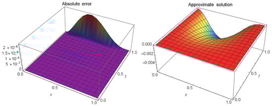
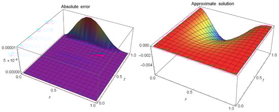
presents a comparison of the maximum absolute errors between our method for $\mathcal{N}=16$ and the method in [57] at different values of ξ when $0<t<1.$ This shows the accuracy of our method. Figure 1 and Figure 2 show the absolute error and approximate solution at different values of α for $\mathcal{N}=16.$ It can be seen that the approximate solutions are quite close to the precise ones.

Example 2.

Consider the following NTFGKE:

$$\begin{array}{cc}\hfill \frac{{\partial }^{\alpha }u(\xi ,t)}{\partial t^{\alpha }}& -\frac{{\partial }^{5}u(\xi ,t)}{\partial {\xi }^5}+\frac{{\partial }^{3}u(\xi ,t)}{\partial {\xi }^3}+u(\xi ,t)\frac{\partial u(\xi ,t)}{\partial \xi }\hfill \\ & +g_1(\xi ,t)\frac{\partial u(\xi ,t)}{\partial \xi }+g_2(\xi ,t)u(\xi ,t)=f(\xi ,t),0\le \xi ,t\le 1,\hfill \end{array}$$

(37)

governed by (20), and $f(\xi ,t)$ is determined in such a way that the exact solution is $u(\xi ,t)=\frac{1}{12}{t}^{1+\alpha }{\xi }^2({\xi }^4-2{\xi }^3+2\xi -1)$.

Equation (37) is solved in two cases corresponding to $g_1(\xi ,t)=1,g_2(\xi ,t)=0$ and $g_1(\xi ,t)=0,g_2(\xi ,t)=1$.

Case 1: At $g_1(\xi ,t)=1$ and $g_2(\xi ,t)=0.$ 

Table 2. Comparison of the maximum absolute errors for $0<t<1$ of Example 2.

	$\mathit{\alpha }=0.7$		$\mathit{\alpha }=0.8$		$\mathit{\alpha }=0.9$
$(\mathit{\xi },\mathit{t})$	Method in [57]	Our Method	Method in [57]	Our Method	Method in [57]	Our Method
(0.1,t)	7.73 $\times {10}^{-6}$	9.87464 $\times {10}^{-8}$	7.98 $\times {10}^{-6}$	4.53983 $\times {10}^{-8}$	8.26 $\times {10}^{-6}$	1.52193 $\times {10}^{-8}$
(0.2,t)	1.57 $\times {10}^{-5}$	3.02778 $\times {10}^{-7}$	1.66 $\times {10}^{-5}$	1.39255 $\times {10}^{-7}$	1.75 $\times {10}^{-5}$	4.67136 $\times {10}^{-8}$
(0.3,t)	1.95 $\times {10}^{-5}$	4.94641 $\times {10}^{-7}$	2.10 $\times {10}^{-5}$	2.27577 $\times {10}^{-7}$	2.26 $\times {10}^{-5}$	7.63871 $\times {10}^{-8}$
(0.4,t)	2.17 $\times {10}^{-5}$	5.96617 $\times {10}^{-7}$	2.12 $\times {10}^{-5}$	2.74586 $\times {10}^{-7}$	2.32 $\times {10}^{-5}$	9.22166 $\times {10}^{-8}$
(0.5,t)	2.09 $\times {10}^{-5}$	5.78239 $\times {10}^{-7}$	1.86 $\times {10}^{-5}$	2.66211 $\times {10}^{-7}$	2.00 $\times {10}^{-5}$	8.94498 $\times {10}^{-8}$
(0.6,t)	1.64 $\times {10}^{-5}$	4.54913 $\times {10}^{-7}$	1.46 $\times {10}^{-5}$	2.09494 $\times {10}^{-7}$	1.44 $\times {10}^{-5}$	7.04262 $\times {10}^{-8}$
(0.7,t)	1.00 $\times {10}^{-5}$	2.77641 $\times {10}^{-7}$	8.90 $\times {10}^{-6}$	1.27891 $\times {10}^{-7}$	8.20 $\times {10}^{-6}$	4.30125 $\times {10}^{-8}$
(0.8,t)	4.10 $\times {10}^{-6}$	1.13802 $\times {10}^{-7}$	3.64 $\times {10}^{-6}$	5.24341 $\times {10}^{-8}$	3.18 $\times {10}^{-6}$	1.76417 $\times {10}^{-8}$
(0.9,t)	6.83 $\times {10}^{-7}$	1.90093 $\times {10}^{-8}$	6.07 $\times {10}^{-7}$	8.75887  $\times {10}^{-9}$	5.27 $\times {10}^{-7}$	2.94852 $\times {10}^{-9}$

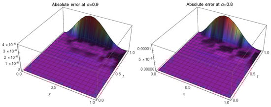
presents a comparison of the maximum absolute errors between our method for $\mathcal{N}=16$ and the method in [57] at different values of x when $0<t<1.$ This shows the accuracy of our method. Further, Figure 3 illustrates the absolute error at different values of α for $\mathcal{N}=16$.

Case 2: At $g_1(\xi ,t)=0$ and $g_2(\xi ,t)=1.$ 

Table 3. The absolute errors of Example 2.

$(\mathit{\xi },\mathit{t})$	$\mathit{\alpha }=0.7$	$\mathit{\alpha }=0.8$	$\mathit{\alpha }=0.9$
(0.1,0.1)	6.7009 $\times {10}^{-10}$	3.0066 $\times {10}^{-10}$	9.7494 $\times {10}^{-11}$
(0.2,0.2)	8.6369 $\times {10}^{-9}$	3.9652 $\times {10}^{-9}$	1.3290 $\times {10}^{-9}$
(0.3,0.3)	5.0761 $\times {10}^{-8}$	2.3250 $\times {10}^{-8}$	7.7603 $\times {10}^{-9}$
(0.4,0.4)	3.8968 $\times {10}^{-7}$	1.7890 $\times {10}^{-7}$	5.9890 $\times {10}^{-8}$
(0.5,0.5)	1.0161 $\times {10}^{-7}$	6.8746 $\times {10}^{-10}$	3.3123 $\times {10}^{-10}$
(0.6,0.6)	4.5491 $\times {10}^{-7}$	2.0949 $\times {10}^{-7}$	7.0426 $\times {10}^{-8}$
(0.7,0.7)	6.9537 $\times {10}^{-8}$	3.2057 $\times {10}^{-8}$	1.0794 $\times {10}^{-8}$
(0.8,0.8)	1.3930 $\times {10}^{-8}$	6.4078 $\times {10}^{-9}$	2.1507 $\times {10}^{-9}$
(0.9,0.9)	1.4303 $\times {10}^{-9}$	6.6288 $\times {10}^{-10}$	2.2524 $\times {10}^{-10}$

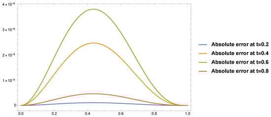
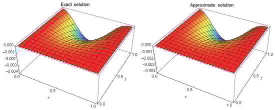
presents the absolute errors at different values of α for $\mathcal{N}=16.$ Figure 4 illustrates the absolute errors at different values of t at $\alpha =0.95$ and $\mathcal{N}=16.$ Figure 5 presents a comparison between the approximate solution and exact solution at $\alpha =0.9$ and $\mathcal{N}=16.$ It can be seen that the approximate solutions are quite near the precise one.

Example 3.

Consider the following NTFGKE:

$$\begin{array}{c}\hfill \frac{{\partial }^{\alpha }u(\xi ,t)}{\partial t^{\alpha }}-\frac{{\partial }^{5}u(\xi ,t)}{\partial {\xi }^5}+\frac{{\partial }^{3}u(\xi ,t)}{\partial {\xi }^3}+u(\xi ,t)\frac{\partial u(\xi ,t)}{\partial \xi }+u(\xi ,t)=f(\xi ,t),0\le \xi ,t\le 1,\end{array}$$

governed by (20), and $f(\xi ,t)$ is chosen such that the exact solution is $u(\xi ,t)={\xi }^2({\xi }^4-2{\xi }^3+2\xi -1)sin\left(2\pi \alpha t\right)$.

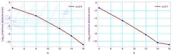
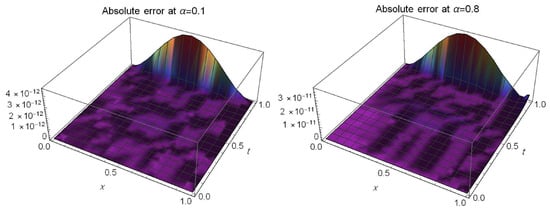
Figure 6 illustrates the ${log}_{10}$(maximum absolute error) at different values of α and $\mathcal{N}$.

Table 4. The absolute errors of Example 3.

	$\mathit{\alpha }=0.5$
$\mathit{\xi }$	$\mathit{t}=\mathbf{0.1}$	$\mathit{t}=\mathbf{0.3}$	$\mathit{t}=\mathbf{0.5}$	$\mathit{t}=\mathbf{0.7}$	$\mathit{t}=\mathbf{0.9}$
0.1	$1.04387\times {10}^{-15}$	$1.87784\times {10}^{-15}$	$9.42649\times {10}^{-15}$	$3.48593\times {10}^{-15}$	$3.20794\times {10}^{-15}$
0.2	$3.25868\times {10}^{-15}$	$5.905\times {10}^{-15}$	$2.94209\times {10}^{-14}$	$1.08559\times {10}^{-14}$	$1.01308\times {10}^{-14}$
0.3	$5.53897\times {10}^{-15}$	$1.00753\times {10}^{-14}$	$4.99947\times {10}^{-14}$	$1.84436\times {10}^{-14}$	$1.73177\times {10}^{-14}$
0.4	$7.12798\times {10}^{-15}$	$1.29688\times {10}^{-14}$	$6.42751\times {10}^{-14}$	$2.36755\times {10}^{-14}$	$2.27804\times {10}^{-14}$
0.5	$7.57207\times {10}^{-15}$	$1.38153\times {10}^{-14}$	$6.82648\times {10}^{-14}$	$2.49592\times {10}^{-14}$	$2.70079\times {10}^{-14}$
0.6	$6.74114\times {10}^{-15}$	$1.24518\times {10}^{-14}$	$6.08194\times {10}^{-14}$	$2.12469\times {10}^{-14}$	$3.71213\times {10}^{-14}$
0.7	$4.87804\times {10}^{-15}$	$9.14546\times {10}^{-15}$	$4.40481\times {10}^{-14}$	$1.12098\times {10}^{-14}$	$9.80414\times {10}^{-14}$
0.8	$2.48412\times {10}^{-15}$	$5.04371\times {10}^{-15}$	$2.24369\times {10}^{-14}$	$2.37137\times {10}^{-15}$	$2.0929\times {10}^{-13}$
0.9	$3.85813\times {10}^{-16}$	$1.75576\times {10}^{-15}$	$4.00461\times {10}^{-15}$	$2.10747\times {10}^{-14}$	$4.78838\times {10}^{-13}$

presents the absolute errors at different values of ξ and t when $\alpha =0.5$ and $\mathcal{N}=16$. Further, Figure 7 illustrates the absolute error at different values of α for $\mathcal{N}=16$.

7. Concluding Remarks

To summarize the principal findings of our study, we present the following insights: Our research encompasses the introduction, implementation, and thorough investigation of a spectral collocation methodology tailored to address the NTFGKE. An in-depth exploration and analysis of convergence are undertaken. Additionally, the outcomes of our work are substantiated through diverse numerical test scenarios. We anticipate that this approach will find application in upcoming endeavors aimed at addressing even more intricate models within the realm of partial differential equations.

In conclusion, the effective utilization of eighth-kind CPs in conjunction with the collocation method is demonstrated through our application to solve the NTFGKE. This showcases the prowess of our spectral approach, affirming its potential for tackling complex mathematical challenges.

References

- Fox, L.; Parker, I.B. Chebyshev Polynomials in Numerical Analysis; Technical Report; Cambridge University Press: Cambridge, UK, 1968. [Google Scholar]
- Mason, J.C.; Handscomb, D.C. Chebyshev Polynomials; Chapman and Hall: New York, NY, USA; CRC: Boca Raton, FL, USA, 2003. [Google Scholar]
- Rivlin, T.J. Chebyshev Polynomials; Courier Dover Publications: New York, NY, USA, 2020. [Google Scholar]
- Thongthai, W.; Nonlaopon, K.; Orankitjaroen, S.; Li, C. Generalized Solutions of Ordinary Differential Equations Related to the Chebyshev Polynomial of the Second Kind. Mathematics 2023, 11, 1725. [Google Scholar] [CrossRef]
- Abdelhakem, M.; Ahmed, A.; Baleanu, D.; El-Kady, M. Monic Chebyshev pseudospectral differentiation matrices for higher-order IVPs and BVPs: Applications to certain types of real-life problems. Comput. Appl. Math. 2022, 41, 253. [Google Scholar] [CrossRef]
- Tural-Polat, S.N.; Dincel, A.T. Numerical solution method for multi-term variable order fractional differential equations by shifted Chebyshev polynomials of the third kind. Alex. Eng. J. 2022, 61, 5145–5153. [Google Scholar] [CrossRef]
- Sweilam, N.H.; Nagy, A.M.; El-Sayed, A.A. On the numerical solution of space fractional order diffusion equation via shifted Chebyshev polynomials of the third kind. J. King Saud Univ. Sci. 2016, 28, 41–47. [Google Scholar] [CrossRef]
- Sakran, M.R.A. Numerical solutions of integral and integro-differential equations using Chebyshev polynomials of the third kind. Appl. Math. Comp. 2019, 351, 66–82. [Google Scholar] [CrossRef]
- Abd-Elhameed, W.M.; Youssri, Y.H. Fifth-kind orthonormal Chebyshev polynomial solutions for fractional differential equations. Comput. Appl. Math. 2018, 37, 2897–2921. [Google Scholar] [CrossRef]
- Abd-Elhameed, W.M.; Youssri, Y.H. Sixth-kind Chebyshev spectral approach for solving fractional differential equations. Int. J. Nonlinear Sci. Numer. Simul. 2019, 20, 191–203. [Google Scholar] [CrossRef]
- Atta, A.G.; Abd-Elhameed, W.M.; Moatimid, G.M.; Youssri, Y.H. Shifted fifth-kind Chebyshev Galerkin treatment for linear hyperbolic first-order partial differential equations. Appl. Numer. Math. 2021, 167, 237–256. [Google Scholar] [CrossRef]
- Atta, A.G.; Abd-Elhameed, W.M.; Youssri, Y.H. Shifted fifth-kind Chebyshev polynomials Galerkin-based procedure for treating fractional diffusion-wave equation. Int. J. Mod. Phys. C 2022, 33, 2250102. [Google Scholar] [CrossRef]
- Atta, A.G.; Abd-Elhameed, W.M.; Moatimid, G.M.; Youssri, Y.H. Modal shifted fifth-kind Chebyshev tau integral approach for solving heat conduction equation. Fractal Fract. 2022, 6, 619. [Google Scholar] [CrossRef]
- Abd-Elhameed, W.M. Novel expressions for the derivatives of sixth kind Chebyshev polynomials: Spectral solution of the non-linear one-dimensional Burgers’ equation. Fractal Frac. 2021, 5, 53. [Google Scholar] [CrossRef]
- Atta, A.G.; Abd-Elhameed, W.M.; Moatimid, G.M.; Youssri, Y.H. Advanced shifted sixth-kind Chebyshev tau approach for solving linear one-dimensional hyperbolic telegraph type problem. Math. Sci. 2022, 1–5. [Google Scholar] [CrossRef]
- Sadri, K.; Aminikhah, H. A new efficient algorithm based on fifth-kind Chebyshev polynomials for solving multi-term variable-order time-fractional diffusion-wave equation. Int. J. Comput. Math. 2022, 99, 966–992. [Google Scholar] [CrossRef]
- Jafari, H.; Nemati, S.; Ganji, R.M. Operational matrices based on the shifted fifth-kind Chebyshev polynomials for solving nonlinear variable order integro-differential equations. Adv. Differ. Equ. 2021, 2021, 435. [Google Scholar] [CrossRef]
- Ganji, R.M.; Jafari, H.; Baleanu, D. A new approach for solving multi variable orders differential equations with Mittag–Leffler kernel. Chaos Solitons Fractals 2020, 130, 109405. [Google Scholar] [CrossRef]
- Ali, K.K.; Abd El Salam, M.A.; Mohamed, M.S. Chebyshev fifth-kind series approximation for generalized space fractional partial differential equations. AIMS Math. 2022, 7, 7759–7780. [Google Scholar] [CrossRef]
- Sadri, K.; Aminikhah, H. Chebyshev polynomials of sixth kind for solving nonlinear fractional PDEs with proportional delay and its convergence analysis. J. Funct. Spaces 2022, 2022, 9512048. [Google Scholar] [CrossRef]
- Babaei, A.; Jafari, H.; Banihashemi, S. Numerical solution of variable order fractional nonlinear quadratic integro-differential equations based on the sixth-kind Chebyshev collocation method. J. Comput. Appl. Math. 2020, 377, 112908. [Google Scholar] [CrossRef]
- Xu, X.; Xiong, L.; Zhou, F. Solving fractional optimal control problems with inequality constraints by a new kind of Chebyshev wavelets method. J. Comput. Sci. 2021, 54, 101412. [Google Scholar] [CrossRef]
- Masjed-Jamei, M. Some New Classes of Orthogonal Polynomials and Special Functions: A Symmetric Generalization of Sturm-Liouville Problems and Its Consequences. Ph.D. Thesis, Department of Mathematics, University of Kassel, Kassel, Germany, 2006. [Google Scholar]
- Abd-Elhameed, W.M.; Alkenedri, A.M. Spectral solutions of linear and nonlinear BVPs using certain Jacobi polynomials generalizing third-and fourth-kinds of Chebyshev polynomials. CMES Comput. Model. Eng. Sci. 2021, 126, 955–989. [Google Scholar] [CrossRef]
- Wang, X.; Wang, J.; Wang, X.; Yu, C. A pseudo-spectral Fourier collocation method for inhomogeneous elliptical inclusions with partial differential equations. Mathematics 2022, 10, 296. [Google Scholar] [CrossRef]
- Li, J. Linear Barycentric rational collocation method for solving non-linear partial differential equations. Inter. J. Appl. Comput. Math. 2022, 8, 236. [Google Scholar] [CrossRef]
- Zheng, X. Numerical approximation for a nonlinear variable-order fractional differential equation via a collocation method. Math. Comput. Simul. 2022, 195, 107–118. [Google Scholar] [CrossRef]
- Zhou, X.; Dai, Y. A spectral collocation method for the coupled system of nonlinear fractional differential equations. AIMS Math. 2022, 7, 5670–5689. [Google Scholar] [CrossRef]
- Kumbinarasaiah, S.; Preetham, M. Applications of the Bernoulli wavelet collocation method in the analysis of MHD boundary layer flow of a viscous fluid. J. Umm Al-Qura Univ. Appl. Sci. 2023, 9, 1–14. [Google Scholar] [CrossRef]
- Xu, M.; Tohidi, E.; Niu, J.; Fang, Y. A new reproducing kernel-based collocation method with optimal convergence rate for some classes of BVPs. Appl. Math. Comput. 2022, 432, 127343. [Google Scholar] [CrossRef]
- Abd-Elhameed, W.M.; Alkhamisi, S.O.; Amin, A.K.; Youssri, Y.H. Numerical contrivance for Kawahara-type differential equations based on fifth-kind Chebyshev polynomials. Symmetry 2023, 15, 138. [Google Scholar] [CrossRef]
- Li, P.; Peng, X.; Xu, C.; Han, L.; Shi, S. Novel extended mixed controller design for bifurcation control of fractional-order Myc/E2F/miR-17-92 network model concerning delay. Math. Methods Appl. Sci. 2023. [Google Scholar] [CrossRef]
- Huang, C.; Wang, J.; Chen, X.; Cao, J. Bifurcations in a fractional-order BAM neural network with four different delays. Neural Netw. 2021, 141, 344–354. [Google Scholar] [CrossRef]
- Ali, Z.; Rabiei, F.; Hosseini, K. A fractal–fractional-order modified Predator–Prey mathematical model with immigrations. Math. Comput. Simul. 2023, 207, 466–481. [Google Scholar] [CrossRef]
- Oldham, K.; Spanier, J. The Fractional Calculus Theory and Applications of Differentiation and Integration to Arbitrary Order; Elsevier: Amsterdam, The Netherlands, 1974. [Google Scholar]
- Kilbas, A.A.; Srivastava, H.M.; Trujillo, J.J. Theory and Applications of Fractional Differential Equations; Elsevier: Amsterdam, The Netherlands, 2006; Volume 204. [Google Scholar]
- Meerschaert, M.M.; Zhang, Y.; Baeumer, B. Particle tracking for fractional diffusion with two time scales. Comput. Math. Appl. 2010, 59, 1078–1086. [Google Scholar] [CrossRef]
- Koeller, R.C. Applications of fractional calculus to the theory of viscoelasticity. J. Appl. Mech. 1984, 51, 299–307. [Google Scholar] [CrossRef]
- Aghdam, Y.E.; Mesgarani, H.; Moremedi, G.; Khoshkhahtinat, M. High-accuracy numerical scheme for solving the space-time fractional advection-diffusion equation with convergence analysis. Alex. Eng. J. 2022, 61, 217–225. [Google Scholar] [CrossRef]
- Hosseini, V.R.; Zou, W. The peridynamic differential operator for solving time-fractional partial differential equations. Nonlinear Dyn. 2022, 109, 1823–1850. [Google Scholar] [CrossRef]
- Zhuang, P.; Liu, F.; Anh, V.; Turner, I. New solution and analytical techniques of the implicit numerical method for the anomalous subdiffusion equation. SIAM J. Numer. Anal. 2008, 46, 1079–1095. [Google Scholar] [CrossRef]
- Adel, M. Numerical simulations for the variable order two-dimensional reaction sub-diffusion equation: Linear and Nonlinear. Fractals 2022, 30, 2240019. [Google Scholar] [CrossRef]
- Sweilam, N.H.; Ahmed, S.M.; Adel, M. A simple numerical method for two-dimensional nonlinear fractional anomalous sub-diffusion equations. Math. Methods Appl. Sci. 2021, 44, 2914–2933. [Google Scholar] [CrossRef]
- Vargas, A.M. Finite difference method for solving fractional differential equations at irregular meshes. Math. Comput. Simul. 2022, 193, 204–216. [Google Scholar] [CrossRef]
- Nadeem, M.; He, J.H. The homotopy perturbation method for fractional differential equations: Part 2, two-scale transform. Int. J. Numer. Methods Heat Fluid Flow 2022, 32, 559–567. [Google Scholar] [CrossRef]
- Alharbi, F.; Zidan, A.; Naeem, M.; Shah, R.; Nonlaopon, K. Numerical investigation of fractional-order differential equations via φ-Haar-wavelet method. J. Funct. Spaces 2021, 2021, 1–14. [Google Scholar] [CrossRef]
- Alquran, M.; Ali, M.; Alshboul, O. Explicit solutions to the time-fractional generalized dissipative Kawahara equation. J. Ocean. Eng. Sci. 2022. [Google Scholar] [CrossRef]
- Alquran, M.; Jaradat, I. A novel scheme for solving Caputo time-fractional nonlinear equations: Theory and application. Nonlinear Dyn. 2018, 91, 2389–2395. [Google Scholar] [CrossRef]
- Baleanu, D.; İnç, M.; Yusuf, A.; Aliyu, A.I. Lie symmetry analysis and conservation laws for the time fractional simplified modified Kawahara equation. Open Phys. 2018, 16, 302–310. [Google Scholar] [CrossRef]
- Wang, G.w.; Liu, X.q.; Zhang, Y.y. Lie symmetry analysis to the time fractional generalized fifth-order KdV equation. Commun. Nonlinear Sci. Numer. Simul. 2013, 18, 2321–2326. [Google Scholar] [CrossRef]
- Podlubny, I. Fractional Differential Equations: An Introduction to Fractional Derivatives, Fractional Differential Equations, to Methods of Their Solution and Some of Their Applications; Elsevier: Amsterdam, The Netherlands, 1998. [Google Scholar]
- Silverman, R. Special Functions and Their Applications; Courier Corporation: New York, NY, USA, 1972. [Google Scholar]
- Xu, Y. An integral formula for generalized Gegenbauer polynomials and Jacobi polynomials. Adv. Appl. Math. 2002, 29, 328–343. [Google Scholar] [CrossRef]
- Draux, A.; Sadik, M.; Moalla, B. Markov–Bernstein inequalities for generalized Gegenbauer weight. Appl. Numer. Math. 2011, 61, 1301–1321. [Google Scholar] [CrossRef]
- Abd-Elhameed, W.M.; Alkhamisi, S.O. New results of the fifth-kind orthogonal Chebyshev polynomials. Symmetry 2021, 13, 2407. [Google Scholar] [CrossRef]
- Koepf, W. Hypergeometric Summation, 2nd ed.; Springer Universitext Series; Springer: Berlin/Heidelberg, Germany, 2014. [Google Scholar]
- Saldır, O.; Sakar, M.; Erdogan, F. Numerical solution of time-fractional Kawahara equation using reproducing kernel method with error estimate. Comput. Appl. Math. 2019, 38, 198. [Google Scholar] [CrossRef]
Disclaimer/Publisher’s Note: The statements, opinions and data contained in all publications are solely those of the individual author(s) and contributor(s) and not of MDPI and/or the editor(s). MDPI and/or the editor(s) disclaim responsibility for any injury to people or property resulting from any ideas, methods, instructions or products referred to in the content. |
© 2023 by the authors. Licensee MDPI, Basel, Switzerland. This article is an open access article distributed under the terms and conditions of the Creative Commons Attribution (CC BY) license (https://creativecommons.org/licenses/by/4.0/).