Article

A Comparative Study of Time Fractional Nonlinear Drinfeld–Sokolov–Wilson System via Modified Auxiliary Equation Method

1
Department of Mathematics, University of the Punjab, Lahore 54590, Pakistan
2
Department of Mathematics, University of Sargodha, Sargodha 40100, Pakistan
3
Department of Computer Science and Mathematics, Lebanese American University, Beirut 1102-2801, Lebanon
4
Department of Mathematics, Art and Science Faculty, Siirt University, Siirt 56100, Turkey
5
Mathematics Research Center, Department of Mathematics, Near East University, Near East Boulevard, Mersin 99138, Turkey
*
Author to whom correspondence should be addressed.
Fractal Fract. 2023, 7(9), 665; https://doi.org/10.3390/fractalfract7090665
Submission received: 15 May 2023 / Revised: 27 August 2023 / Accepted: 31 August 2023 / Published: 3 September 2023

Abstract

:
The time-fractional nonlinear Drinfeld–Sokolov–Wilson system, which has significance in the study of traveling waves, shallow water waves, water dispersion, and fluid mechanics, is examined in the presented work. Analytic exact solutions of the system are produced using the modified auxiliary equation method. The fractional implications on the model are examined under β -fractional derivative and a new fractional local derivative. Extracted solutions include rational, trigonometric, and hyperbolic functions with dark, periodic, and kink solitons. Additionally, by specifying values for fractional parameters, graphs are utilized to comprehend the fractional effects on the obtained solutions.

1. Introduction

Fractional calculus (FC) is a branch of mathematics that generalizes the concept of differentiation and integration to non-integer orders. It has applications in many fields, including physics, engineering, finance, and signal processing. FC provides a more accurate way to model complex systems that exhibit non-local, long-term memory effects. This includes phenomena such as anomalous diffusion, fractional Brownian motion, and viscoelastic materials. In control theory, FC can be used to design advanced control systems for complex physical systems, such as robotics and industrial processes. The fractional derivative of a system’s output signal can provide valuable information about the system’s behavior, which can be used to design more effective controllers. FC has great use in the telecommunication industry. It provides a powerful tool for analyzing and processing signals that exhibit non-local memory effects, such as speech and image processing. Fractional differentiation and integration can be used to extract useful information from signals and remove unwanted noise. FC has been used to develop advanced models for analyzing financial markets, such as fractional Black-Scholes models and fractional stochastic volatility models. It has been used in electrochemistry to study electrochemical kinetics and transport processes in electrochemical systems, including battery systems. Overall, FC provides a powerful tool for modeling and analyzing complex systems and processes that exhibit non-local, long-term memory effects. Its applications are far-reaching and span many different fields of science and engineering [1,2].
Fractional models of PDEs offer a powerful mathematical tool to describe physical phenomena that exhibit non-local interactions, long-range correlations, memory effects, or fractal properties. By incorporating fractional derivatives or integrals, these models provide more accurate and comprehensive descriptions of various natural processes, extending beyond the limitations of classical PDEs. The β -fractional derivative and the new local fractional derivative are two relatively new definitions of fractional derivative that offer alternative approaches to describe physical systems with memory effects and fractal properties. By extending the concept of differentiation to non-integer orders and incorporating these derivatives into mathematical models, a more comprehensive understanding of complex physical phenomena can be achieved.
The Drinfeld–Sokolov–Wilson (DSW) nonlinear system is a coupled system of partial differential equations that arises in the study of solitons and integrable systems. Wilson first proposed the DSW system as a generalization of the Korteweg–de Vries (KdV) equation. Mathematical representation of the fractional DSW system is:
0 A D t β U + α V V x = 0 , 0 A D t β V + s V U x + r U V x + η V x x x = 0 ,
where 0 A D t β denotes the time fractional differential operator. In system (1), U : R × R R is an arbitrary function [3,4] such that U and its first order partial derivatives with respect to t and x are continuous on the domain R × R . Moreover, V : R × R R is an arbitrary function such that V, its first order partial derivative with respect to t, and third order partial derivatives with respect to x are continuous on the domain R × R . The considered system of differential equations is solved on the whole domain R × R , where the constraint conditions for the parameters must be satisfied for the existence of solutions. Moreover, α , s , r , and η are real constants. Applications of the coupled DSW-system appear in the study of traveling waves, shallow water waves, water dispersion, and fluid mechanics, which can be studied using the concept of a fractional derivative in a much better way due to the flexibility of the fractional order differential operators. In the limiting case, the fractional order system converges to the integer order system as the fractional parameter approaches unity. The physical significance of the DSW system extends beyond its mathematical elegance. It has been found to have applications in various areas of physics, including condensed matter physics, quantum field theory, and string theory. The soliton solutions and integrability properties of the DSW equation provide insights into phenomena such as magnetic flux quantization, quantum Hall effects, and topological excitations in high-energy physics. The Drinfeld–Sokolov–Wilson (DSW) nonlinear system is a mathematical model that describes the dynamics of a field taking values in a Lie algebra. It is a highly integrable system with soliton solutions and is of interest in both theoretical and applied physics, contributing to the understanding of fundamental phenomena in various fields. Over the years, many researchers have studied this system using various mathematical techniques and approaches. One of the early works on the DSW system was carried out by Wilson. He showed that the DSW system has a rich set of symmetries that are related to the affine Lie algebra of type A1. This work laid the foundation for further studies on the DSW system using Lie algebra and symmetry methods. Naz, using the multiplier approach, developed conservation laws for the DSW system [5]. These conservation laws are useful in understanding the dynamics of the system and can also be used to construct exact solutions. Zhang employed the variational method to study the DSW system and earned solitary solutions and singular periodic solutions [6]. Morris and Kara showed that the formulation that associates conservation laws and symmetries leads to double reduction in the case of the DSW system [7]. Zhao et al. used Lie symmetry analysis to obtain the Lie algebra and similarity reductions for the DSW system [8]. Jaradat et al. obtained approximate solutions for the time fractional DSW system using the Riemann–Liouville fractional derivative and the reduced polynomial method. This approach provides a systematic way of finding approximate solutions for the system [9]. Tasbozan employed the sine-Gordon expansion method and perturbation iteration method to calculate exact and approximate analytical solutions of the time fractional conformable DSW system [10]. Singh et al. examined the Caputo DSW system via the homotopy analysis Sumudu transformation method [11]. This method allows the construction of exact solutions for the system. Gao et al. studied the time fractional DSW system under the AB fractional derivative using an amalgamation of q-homotopy analysis scheme and Laplace transformation methodology [12]. Srivastava and Saad employed the Adomian decomposition method to study the fractional version of the DSW system under numerous fractional derivatives. This approach provides a powerful tool for finding approximate solutions for the system [13]. Rozbayani and Ali explored the system under a combination of Sumudu transform and Adomian decomposition method [14]. Recently, the fractional DSW system has been examined with Mittage–Laffler type kernels and exponential decay. This work provides insight into the behavior of the system when the fractional derivative is replaced by a different kernel function [15]. There are numerous exact approaches that can still be used to study the time fractional DSW system. In the future, some powerful methods, including the variational method [16], Sardar subequation method [17], and Wang’s Bäcklund transformation-based method [18] could further serve as good mathematical tools to study the system. Wang’s Bäcklund transformation-based method is a new method that converts fractional PDE into an ODE using a new transformation and derives solutions involving four different functions [19]. Overall, the study of the DSW system offers insights into the behavior of nonlinear systems. The use of symmetry and algebraic methods, as well as fractional calculus, has provided a deeper understanding of the dynamics of the system and the properties of the solutions.
The main focus of the presented study is to investigate the nonlinear Drinfeld–Sokolov–Wilson (DSW) system using the concept of β -fractional derivative and a new local fractional derivative via modified auxiliary equation method. It is the first time that a fractional nonlinear DSW system is being studied under the effect of β -fractional derivative and new local fractional derivative using the modified auxiliary equation method. The suggested methodology is proficient, easy to proceed, and reliable for extracting analytic exact solutions of fractional nonlinear partial differential equations. This method can generate a variety of closed form solutions, including trigonometric, hyperbolic, and rational functions. Theoretically, various types of traveling wave solutions can be obtained by assigning arbitrary values to free parameters appearing in the aforementioned technique for the considered DSW system. In the laboratory, these solutions can be used as prior knowledge to generate desired possible soliton pulses in fluids.
The work being offered is organized as follows: Understanding of the fundamental ideas for β -fractional derivative and new local fractional derivative is provided in Section 2. Section 3 describes the MAE method in detail. In Section 4, the MAE method is employed to provide exact solutions for the time fractional nonlinear DSW system. Discussion on the obtained traveling structures is presented in Section 5, and the general conclusion is drawn in Section 6.

2. Fundamentals of Fractional Derivatives

There have been several definitions of fractional derivatives developed over the years. Almost all the presented definitions are unable to satisfy one or more mathematical properties of differential operators in classical calculus or they are too complicated to apply in theoretical investigations. The β -fractional derivative and new local fractional derivative are recently developed definitions of fractional derivative which satisfy almost all the properties of the integer order derivative. Owing to the useful mathematical properties of the beta fractional derivative and new local fractional derivative, these definitions of fractional derivatives are more suitable for obtaining new results for real life applications. Some key ideas of FC that have been exercised in the presented study are included in this section.

2.1. β -Derivative

Definition 1
([20,21]). Atangana et al. introduced the β-fractional derivative for the first time in 2016. Let F : [ a , ) R be an arbitrary function. Then the β-fractional derivative of F is defined, as:
0 A D t β F ( t ) = lim ϵ 0 F t + ϵ t + 1 Γ ( β ) 1 β F ( t ) ϵ ,
for all t a , 0 < β 1 .
If the limit in Equation (2) exists, then F is said to be β-differentiable. Here, Γ ( β ) is the well-known gamma function defined by Γ ( β ) = 0 t β 1 e t d t . The gamma function is the generalization of the factorial function to non-integer numbers.
The β-derivative has the following properties:
0 A D t β l F ( t ) + m G ( t ) = l l A D t β F ( t ) + m l A D t β G ( t ) , l , m R , 0 A D t β F ( t ) G ( t ) = G ( t ) l A D t β F ( t ) + F ( t ) l A D t β G ( t ) , 0 A D t β F ( t ) G ( t ) = G ( t ) l A D t β F ( t ) F ( t ) l A D t β G ( t ) G 2 ( t ) , 0 A D t β γ = 0 , w h e r e   γ   i s   a   c o n s t a n t .
If F is a differentiable function, then substituting ϵ = t + 1 Γ ( β ) β 1 b , b 0 when ϵ 0 , Equation (2) can be written as
0 A D t β ( F ( t ) ) = t + 1 Γ ( β 1 β lim b 0 F t + b F ( t ) b , = t + 1 Γ ( β 1 β d F ( t ) d t .
This characteristic of β-fractional derivative is the main key that enables the use of any exact analytic approach to derive specific results for the time fractional nonlinear DSW system (1).
The  β -fractional integral is defined as:
0 A I x β F ( x ) = 0 x ϖ + 1 Γ [ β ] β 1 F ( ϖ ) d ϖ .

2.2. A New Fractional Local Derivative

Definition 2.
For all 0 < t , the new local fractional derivative is defined as
N h y p β F ( t ) = lim ϵ 0 F t + ϵ t 1 β 2 sech ( 1 β ) t 1 + β 2 F ( t ) ϵ , 0 < β < 1 .
A similar operator, N 1 β F ( t ) , is studied in [22]. It can be noticed that for F : [ a 1 , a 2 ] R with a 1 < t , if the limit lim t a 1 + N h y p β F ( t ) exists, then
N h y p β F ( a 1 ) = lim t a 1 + N h y p β F ( t )
and F is β-differentiable at  a 1  with respect to N h y p β F ( t ) . The new fractional local derivative satisfies one important result, i.e.,
N h y p β F ( t ) = t 1 β 2 sech ( 1 β ) t 1 + β 2 d F ( t ) d t ,
in which F : [ a 1 , a 2 ] R is differentiable for a 1 < t . The properties stated in [22] for the N 1 β F ( t ) can be straightforwardly generalized to obtain Equation (4), and the following identity, which has been proven in [23], is satisfied:
N h y p β 2 1 β 2 sinh ( 1 β ) t 1 + β 2 = 1 .
The chain rule
N h y p β ( F . G ) ( t ) = F ( G ( t ) ) N h y p β G ( t ) ,
holds. From Equations (5) and (6), it can be written as
N h y p β F ( Λ ) = ς F ( Λ ) ,
with
Λ = 2 1 β 2 sinh ( 1 β ) ς t 1 + β 2 ,
for the constant ς. This final finding is essential in the search of exact results for the fractional DSW system.

3. Details of Suggested Methodology

Consider the nonlinear partial differential equation (NPDE) as
Q ( Q , Q x , Q t , Q x x , Q x t , ) = 0 ,
where Q = Q ( x , t ) is a solution of NPDE (9).
Making use of the transformation
Q ( x , t ) = q ( χ ) ,
Equation (9) can be transformed into an ordinary differential equation by defining χ with respect to the considered fractional derivative as
R ( q , q , q , ) = 0 ,
where q = d q d χ .
For β -derivative,
χ = 1 β x + 1 Γ ( β ) β ω β t + 1 Γ ( β ) β .
For new local fractional derivative,
χ = 2 1 β 2 sinh ( 1 β ) ( x 1 + β 2 ω t 1 + β 2 ,
where ω is used as a real constant.
The MAE method [24,25,26] assumes the general solution of Equation (11) as
φ ( χ ) = p 0 + i = 1 p i ( h z ) i + q i ( h z ) i ,
where p i s, q i s are constants to be calculated and z ( χ ) follows the auxiliary equation
z ( χ ) = η 1 + η 0 h z + η 2 h z ln h .
Here η 0 , η 1 , η 2 , and h are arbitrary constants with h > 0 , h 1 . The solutions of Equation (15) are as follows:
  • If η 1 2 4 η 0 η 2 < 0 and η 2 0 ,
h z ( χ ) = η 1 + 4 η 0 η 2 η 1 2 tan ( 4 η 0 η 2 η 1 2 χ 2 ) 2 η 2 or h z ( χ ) = η 1 + 4 η 0 η 2 η 1 2 cot ( 4 η 0 η 2 η 1 2 χ 2 ) 2 η 2 .
  • If η 1 2 4 η 0 η 2 > 0 and η 2 0 ,
h z ( χ ) = η 1 + η 1 2 4 η 0 η 2 tanh ( η 1 2 4 η 0 η 2 χ 2 ) 2 η 2 or h z ( χ ) = η 1 + η 1 2 4 η 0 η 2 coth ( η 1 2 4 η 0 η 2 χ 2 ) 2 η 2 .
  • If η 1 2 4 η 0 η 2 = 0 and η 2 0 ,
h z ( χ ) = 2 + η 1 χ 2 η 2 χ .

4. Construction of Solutions via Modified Auxiliary Equation Method

Considering the traveling wave transformation (10) along with Equations (12) and (13) in system (1) gives
ω U + α V V = 0
and
ω V + s V U + r U V + η V = 0 .
Simplification of Equations (16) and (17) gives
U = α V 2 2 ω
and
6 η ω V + α ( 2 s + r ) V 3 6 ω 2 V = 0 .
Balancing the degrees of V and V 3 in Equation (19) gives = 1 . The general solution of Equation (19) according to MAE method takes the form
V ( χ ) = p 0 + p 1 h z + q 1 h z .
Inserting Equation (20) into Equation (19), along with Equation (15) and equating coefficients of all powers of h z to zero, yields a system of algebraic equations. The possible solutions of the system are
Family 1 : { ω = 1 2 η 4 η 0 η 2 η 1 2 , p 0 = 1 2 24 η 0 η 2 6 η 1 2 α r + 2 α s η η 1 , p 1 = 0 , q 1 = 24 η 0 η 2 6 η 1 2 α r + 2 α s η 0 η } .
Family 2 : { ω = 1 2 η 4 η 0 η 2 η 1 2 , p 0 = 1 2 24 η 0 η 2 6 η 1 2 α r + 2 α s η η 1 , p 1 = 24 η 0 η 2 6 η 1 2 α r + 2 α s η 2 η , q 1 = 0 } .
Family 3 : { ω = 1 4 F η , p 0 = 18 3 α r + 2 s F η 2 η η 0 η 1 α r + 2 s 3 F r r + 2 s + 6 F s r + 2 s 12 η 0 η 2 6 η 1 2 , p 1 = 3 α r + 2 s F η 2 η α r + 2 s , q 1 = 0 } .
where   F = 4 η 0 η 2 η 1 2 + 3 8 η 0 η 1 2 η 2 + η 1 4 . The solutions of the DSW-system corresponding to family 1 are
  • If η 1 2 4 η 0 η 2 < 0 and η 2 0 ,
U 11 ( χ ) = α η 4 η 0 η 2 η 1 2 1 2 24 η 0 η 2 6 η 1 2 α r + 2 α s η η 1 + 2 η 0 η η 2 η 1 + 4 η 0 η 2 η 1 2 tan 1 2 4 η 0 η 2 η 1 2 χ 24 η 0 η 2 6 η 1 2 α r + 2 α s 2
or
U 11 ( χ ) = α η 4 η 0 η 2 η 1 2 1 2 24 η 0 η 2 6 η 1 2 α r + 2 α s η η 1 2 η 0 η η 2 η 1 + 4 η 0 η 2 η 1 2 cot 1 2 4 η 0 η 2 η 1 2 χ 24 η 0 η 2 6 η 1 2 α r + 2 α s 2
and
V 11 ( χ ) = 1 2 24 η 0 η 2 6 η 1 2 α r + 2 α s η η 1 + 2 η 0 η η 2 η 1 + 4 η 0 η 2 η 1 2 tan 1 2 4 η 0 η 2 η 1 2 χ 24 η 0 η 2 6 η 1 2 α r + 2 α s
or
V 11 ( χ ) = 1 2 24 η 0 η 2 6 η 1 2 α r + 2 α s η η 1 2 η 0 η η 2 η 1 + 4 η 0 η 2 η 1 2 cot 1 2 4 η 0 η 2 η 1 2 χ 24 η 0 η 2 6 η 1 2 α r + 2 α s .
  • If η 1 2 4 η 0 η 2 > 0 and η 2 0 ,
U 12 ( χ ) = α η 4 η 0 η 2 η 1 2 1 2 24 η 0 η 2 6 η 1 2 α r + 2 α s η η 1 2 η 0 η η 2 η 1 + 4 η 0 η 2 + η 1 2 tanh 1 2 4 η 0 η 2 + η 1 2 χ 24 η 0 η 2 6 η 1 2 α r + 2 α s 2
or
U 12 ( χ ) = α η 4 η 0 η 2 η 1 2 1 2 24 η 0 η 2 6 η 1 2 α r + 2 α s η η 1 2 η 0 η η 2 η 1 + 4 η 0 η 2 + η 1 2 coth 1 2 4 η 0 η 2 + η 1 2 χ 24 η 0 η 2 6 η 1 2 α r + 2 α s 2
and
V 12 ( χ ) = 1 2 24 η 0 η 2 6 η 1 2 α r + 2 α s η η 1 2 η 0 η η 2 η 1 + 4 η 0 η 2 + η 1 2 tanh 1 2 4 η 0 η 2 + η 1 2 χ 24 η 0 η 2 6 η 1 2 α r + 2 α s
or
V 12 ( χ ) = 1 2 24 η 0 η 2 6 η 1 2 α r + 2 α s η η 1 2 η 0 η η 2 η 1 + 4 η 0 η 2 + η 1 2 coth 1 2 4 η 0 η 2 + η 1 2 χ 24 η 0 η 2 6 η 1 2 α r + 2 α s .
Here, the constraint condition r 2 s must hold for the existence of solutions.
The solutions of DSW-system corresponding to family 2 are
  • If η 1 2 4 η 0 η 2 < 0 and η 2 0 ,
U 21 ( χ ) = α η 4 η 0 η 2 η 1 2 1 2 24 η 0 η 2 6 η 1 2 α r + 2 α s η η 1 + 1 2 24 η 0 η 2 6 η 1 2 α r + 2 α s η η 1 + 4 η 0 η 2 η 1 2 tan 1 2 4 η 0 η 2 η 1 2 χ 2
or
U 21 ( χ ) = α η 4 η 0 η 2 η 1 2 1 2 24 η 0 η 2 6 η 1 2 α r + 2 α s η η 1 1 2 24 η 0 η 2 6 η 1 2 α r + 2 α s η η 1 + 4 η 0 η 2 η 1 2 cot 1 2 4 η 0 η 2 η 1 2 χ 2
and
V 21 ( χ ) = 1 2 24 η 0 η 2 6 η 1 2 α r + 2 α s η η 1 + 1 2 24 η 0 η 2 6 η 1 2 α r + 2 α s η η 1 + 4 η 0 η 2 η 1 2 tan 1 2 4 η 0 η 2 η 1 2 χ
or
V 21 ( χ ) = 1 2 24 η 0 η 2 6 η 1 2 α r + 2 α s η η 1 1 2 24 η 0 η 2 6 η 1 2 α r + 2 α s η η 1 + 4 η 0 η 2 η 1 2 cot 1 2 4 η 0 η 2 η 1 2 χ .
  • If η 1 2 4 η 0 η 2 > 0 and η 2 0 ,
U 22 ( χ ) = α η 4 η 0 η 2 η 1 2 1 2 24 η 0 η 2 6 η 1 2 α r + 2 α s η η 1 1 2 24 η 0 η 2 6 η 1 2 α r + 2 α s η η 1 + 4 η 0 η 2 + η 1 2 tanh 1 2 4 η 0 η 2 + η 1 2 χ 2
or
U 22 ( χ ) = α η 4 η 0 η 2 η 1 2 1 2 24 η 0 η 2 6 η 1 2 α r + 2 α s η η 1 1 2 24 η 0 η 2 6 η 1 2 α r + 2 α s η η 1 + 4 η 0 η 2 + η 1 2 coth 1 2 4 η 0 η 2 + η 1 2 χ 2
and
V 22 ( χ ) = 1 2 24 η 0 η 2 6 η 1 2 α r + 2 α s η η 1 1 2 24 η 0 η 2 6 η 1 2 α r + 2 α s η η 1 + 4 η 0 η 2 + η 1 2 tanh 1 2 4 η 0 η 2 + η 1 2 χ
or
V 22 ( χ ) = 1 2 24 η 0 η 2 6 η 1 2 α r + 2 α s η η 1 1 2 24 η 0 η 2 6 η 1 2 α r + 2 α s η η 1 + 4 η 0 η 2 + η 1 2 coth 1 2 4 η 0 η 2 + η 1 2 χ .
Here, the constraint condition r 2 s must hold for the existence of solutions.
The solutions of DSW-system corresponding to family 3 are
  • If η 1 2 4 η 0 η 2 < 0 and η 2 0 ,
U 31 ( χ ) = 2 α F η 18 3 α r + 2 s F η 2 η η 0 η 1 α r + 2 s 3 F r r + 2 s + 6 F s r + 2 s 12 η 0 η 2 6 η 1 2 + 1 2 3 α r + 2 s F η η 1 + 4 η 0 η 2 η 1 2 tan 1 2 4 η 0 η 2 η 1 2 χ α r + 2 s 2
or
U 31 ( χ ) = 2 α F η 18 3 α r + 2 s F η 2 η η 0 η 1 α r + 2 s 3 F r r + 2 s + 6 F s r + 2 s 12 η 0 η 2 6 η 1 2 1 2 3 α r + 2 s F η η 1 + 4 η 0 η 2 η 1 2 cot 1 2 4 η 0 η 2 η 1 2 χ α r + 2 s 2
and
V 31 ( χ ) = 18 3 α r + 2 s F η 2 η η 0 η 1 α r + 2 s 3 F r r + 2 s + 6 F s r + 2 s 12 η 0 η 2 6 η 1 2 + 1 2 3 α r + 2 s F η η 1 + 4 η 0 η 2 η 1 2 tan 1 2 4 η 0 η 2 η 1 2 χ α r + 2 s
or
V 31 ( χ ) = 18 3 α r + 2 s F η 2 η η 0 η 1 α r + 2 s 3 F r r + 2 s + 6 F s r + 2 s 12 η 0 η 2 6 η 1 2 1 2 3 α r + 2 s F η η 1 + 4 η 0 η 2 η 1 2 cot 1 2 4 η 0 η 2 η 1 2 χ α r + 2 s .
  • If η 1 2 4 η 0 η 2 > 0 and η 2 0 ,
U 32 ( χ ) = 2 α F η 18 3 α r + 2 s F η 2 η η 0 η 1 α r + 2 s 3 F r r + 2 s + 6 F s r + 2 s 12 η 0 η 2 6 η 1 2 1 2 3 α r + 2 s F η η 1 + 4 η 0 η 2 + η 1 2 tanh 1 2 4 η 0 η 2 + η 1 2 χ α r + 2 s 2
or
U 32 ( χ ) = 2 α F η 18 3 α r + 2 s F η 2 η η 0 η 1 α r + 2 s 3 F r r + 2 s + 6 F s r + 2 s 12 η 0 η 2 6 η 1 2 1 2 3 α r + 2 s F η η 1 + 4 η 0 η 2 + η 1 2 coth 1 2 4 η 0 η 2 + η 1 2 χ α r + 2 s 2
and
V 32 ( χ ) = 18 3 α r + 2 s F η 2 η η 0 η 1 α r + 2 s 3 F r r + 2 s + 6 F s r + 2 s 12 η 0 η 2 6 η 1 2 1 2 3 α r + 2 s F η η 1 + 4 η 0 η 2 + η 1 2 tanh 1 2 4 η 0 η 2 + η 1 2 χ α r + 2 s
or
V 32 ( χ ) = 18 3 α r + 2 s F η 2 η η 0 η 1 α r + 2 s 3 F r r + 2 s + 6 F s r + 2 s 12 η 0 η 2 6 η 1 2 1 2 3 α r + 2 s F η η 1 + 4 η 0 η 2 + η 1 2 coth 1 2 4 η 0 η 2 + η 1 2 χ α r + 2 s .
  • If η 1 2 4 η 0 η 2 = 0 and η 2 0 ,
U 33 ( χ ) = 2 α F γ 18 3 α r + 2 s F η 2 η η 0 η 1 α r + 2 s 3 F r r + 2 s + 6 F s r + 2 s 12 η 0 η 2 6 η 1 2 3 α r + 2 s F η χ η 1 + 2 2 α r + 2 s χ 2
and
V 33 ( χ ) = 18 3 α r + 2 s F η 2 η η 0 η 1 α r + 2 s 3 F r r + 2 s + 6 F s r + 2 s 12 η 0 η 2 6 η 1 2 3 α r + 2 s F η χ η 1 + 2 2 α r + 2 s χ .
Here, the constraint condition r 2 s must hold for the existence of solutions.

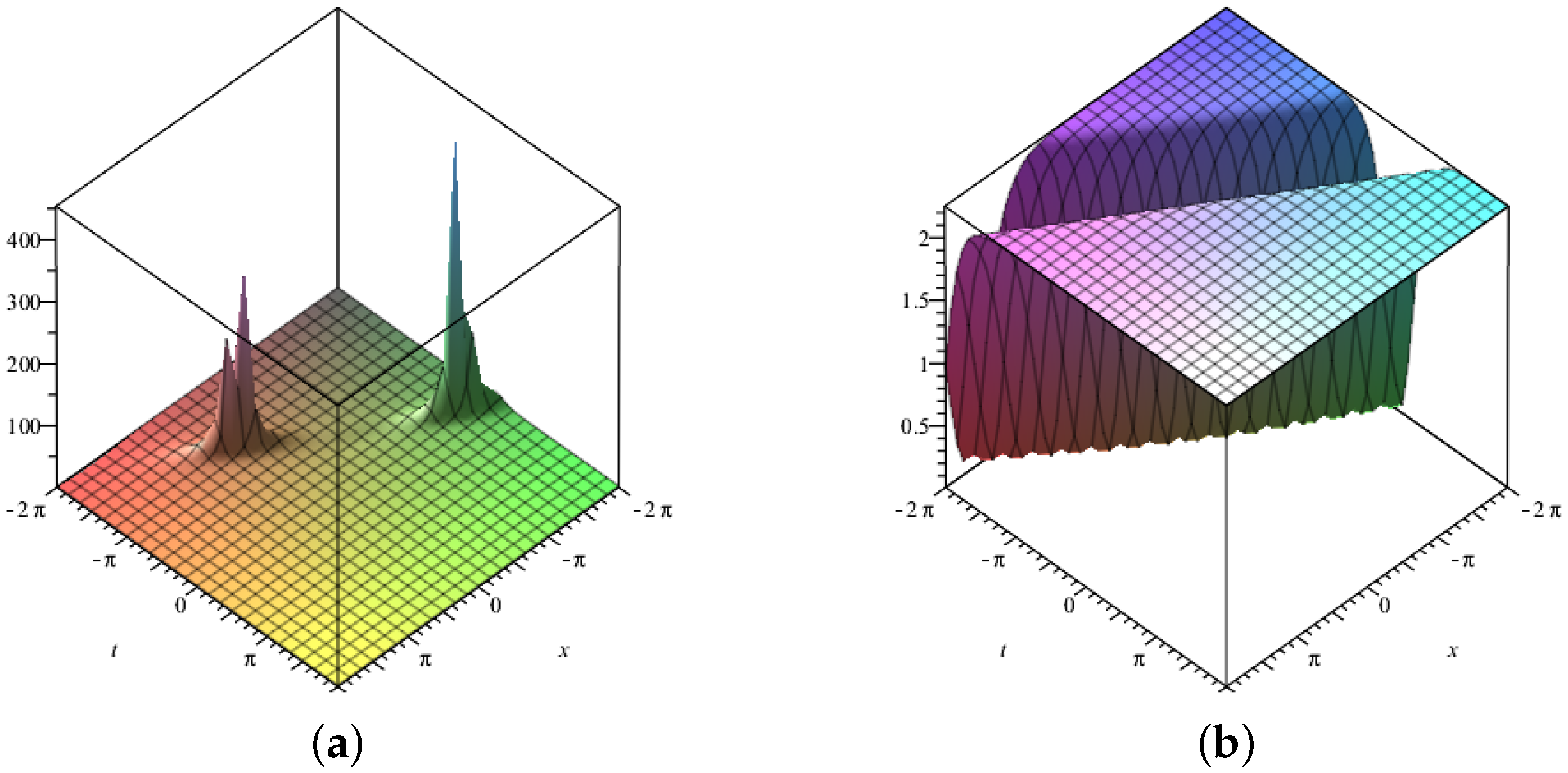
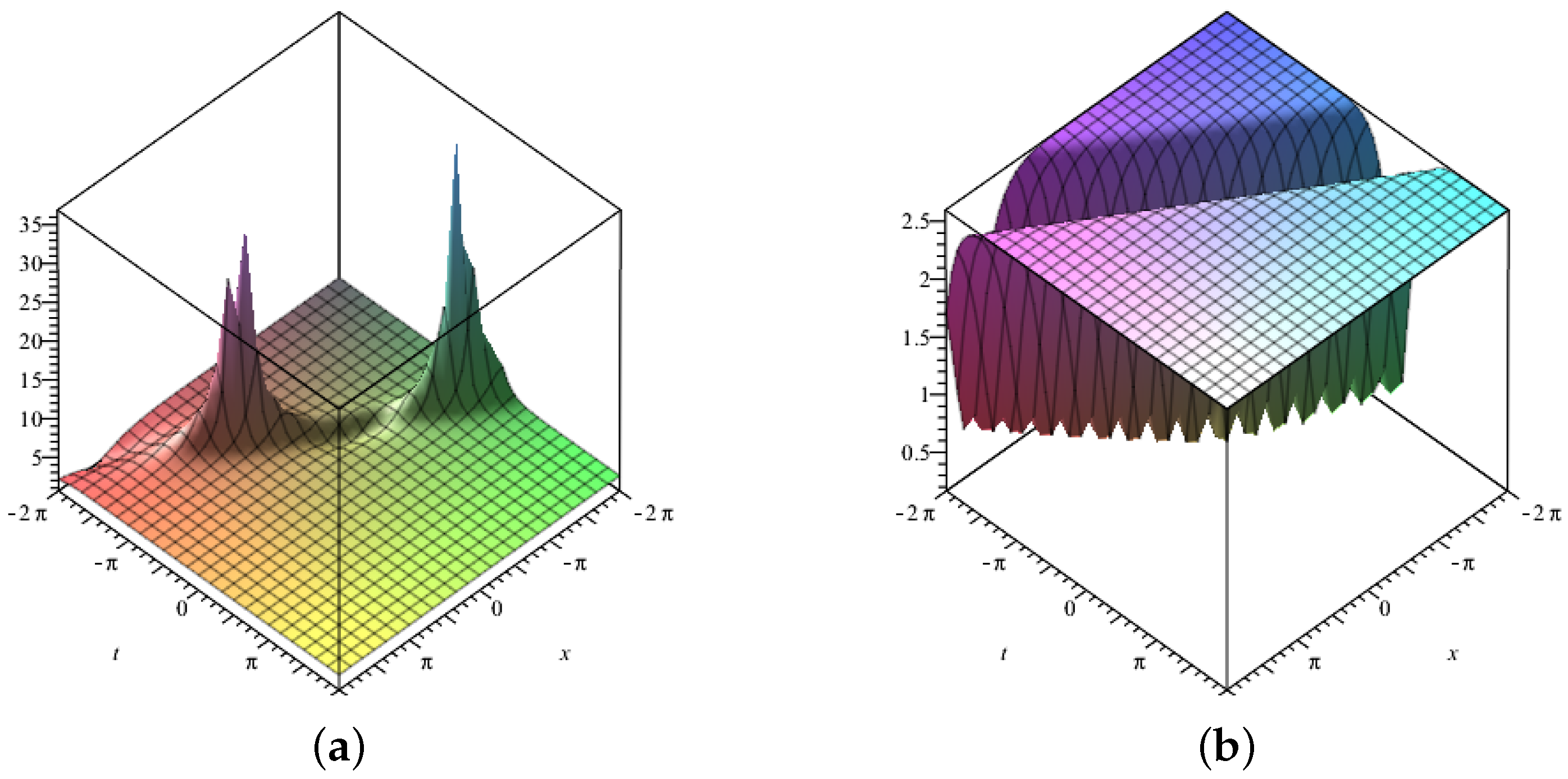
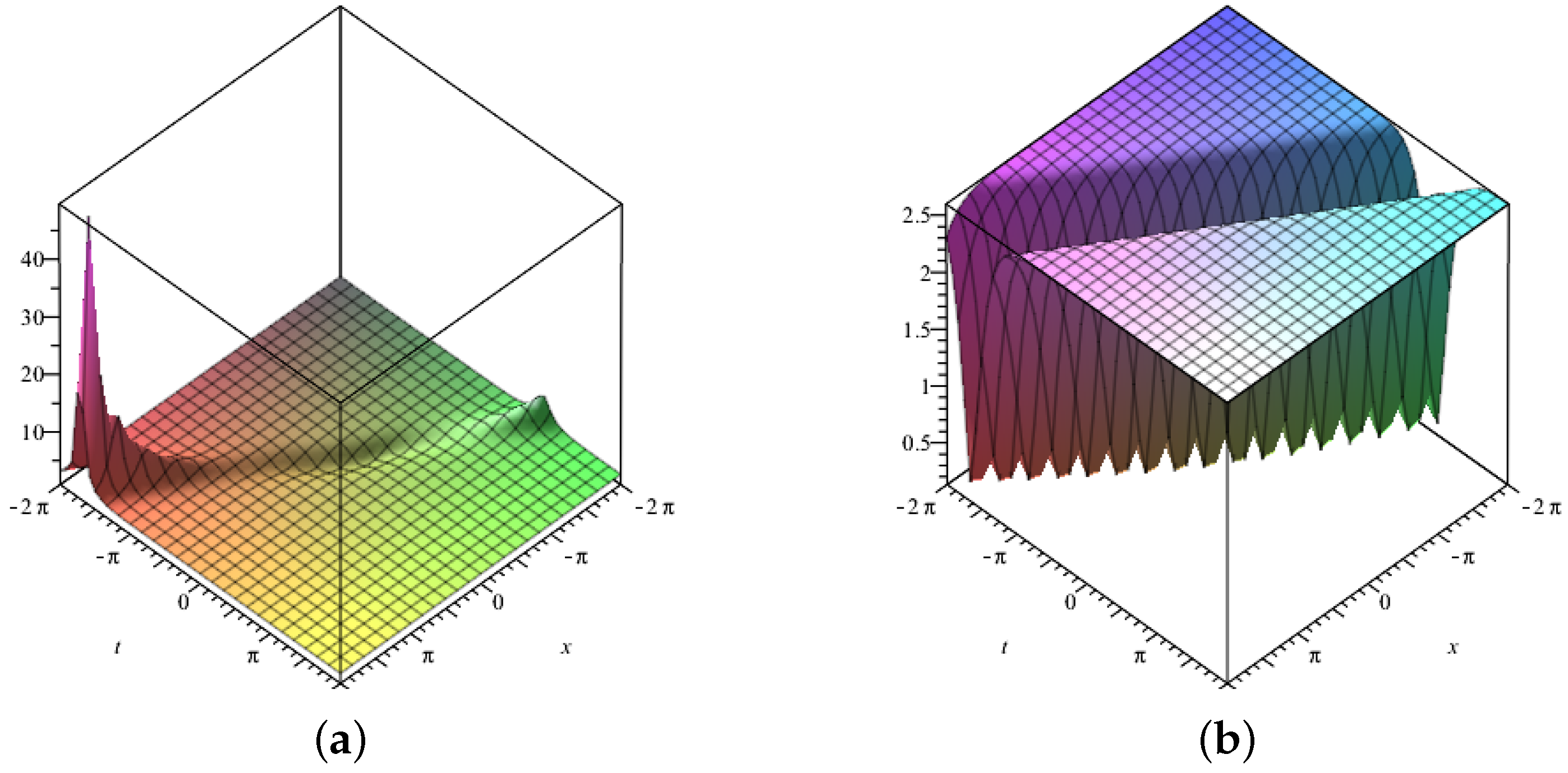
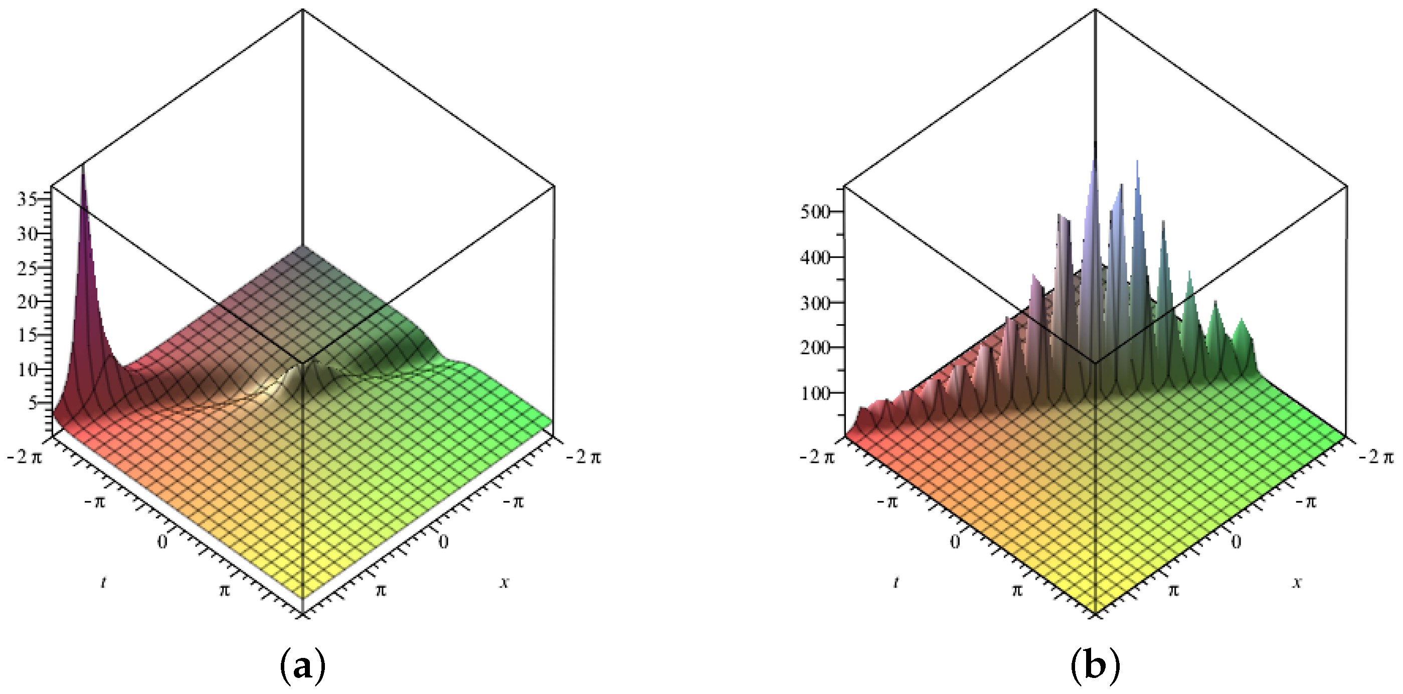
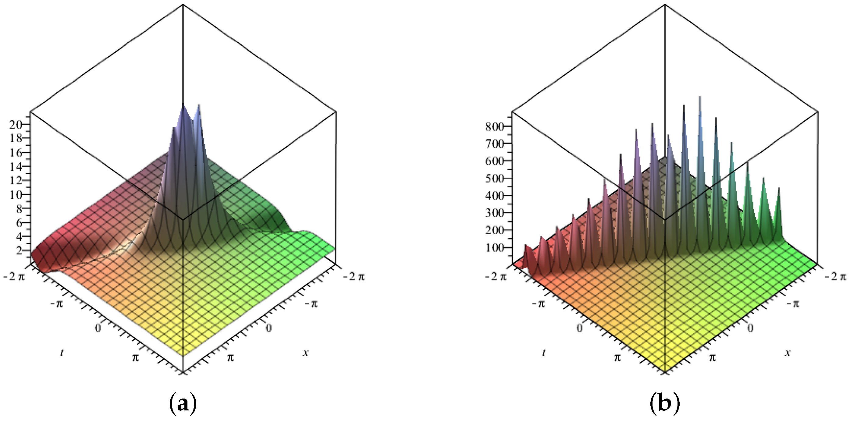
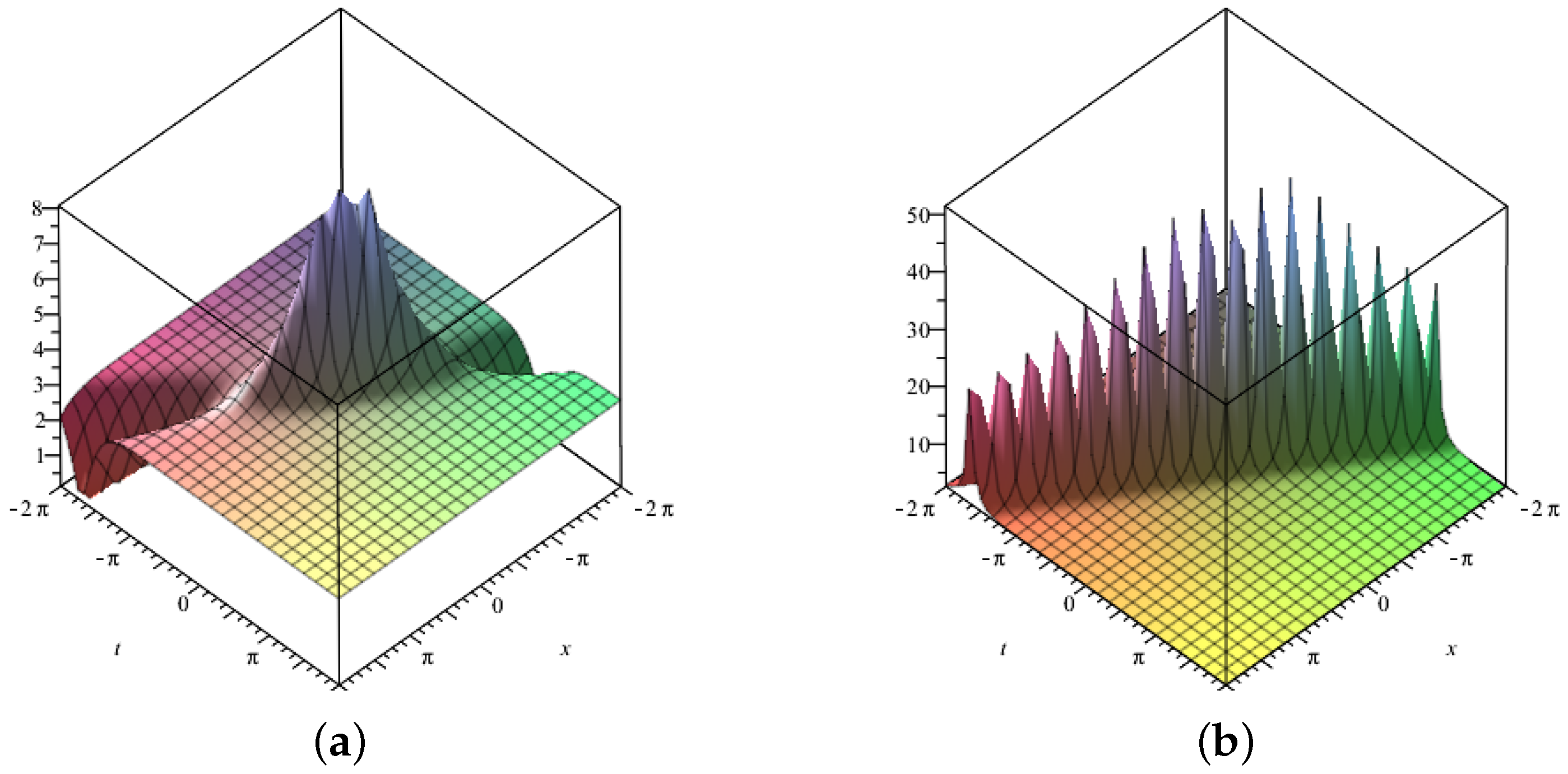
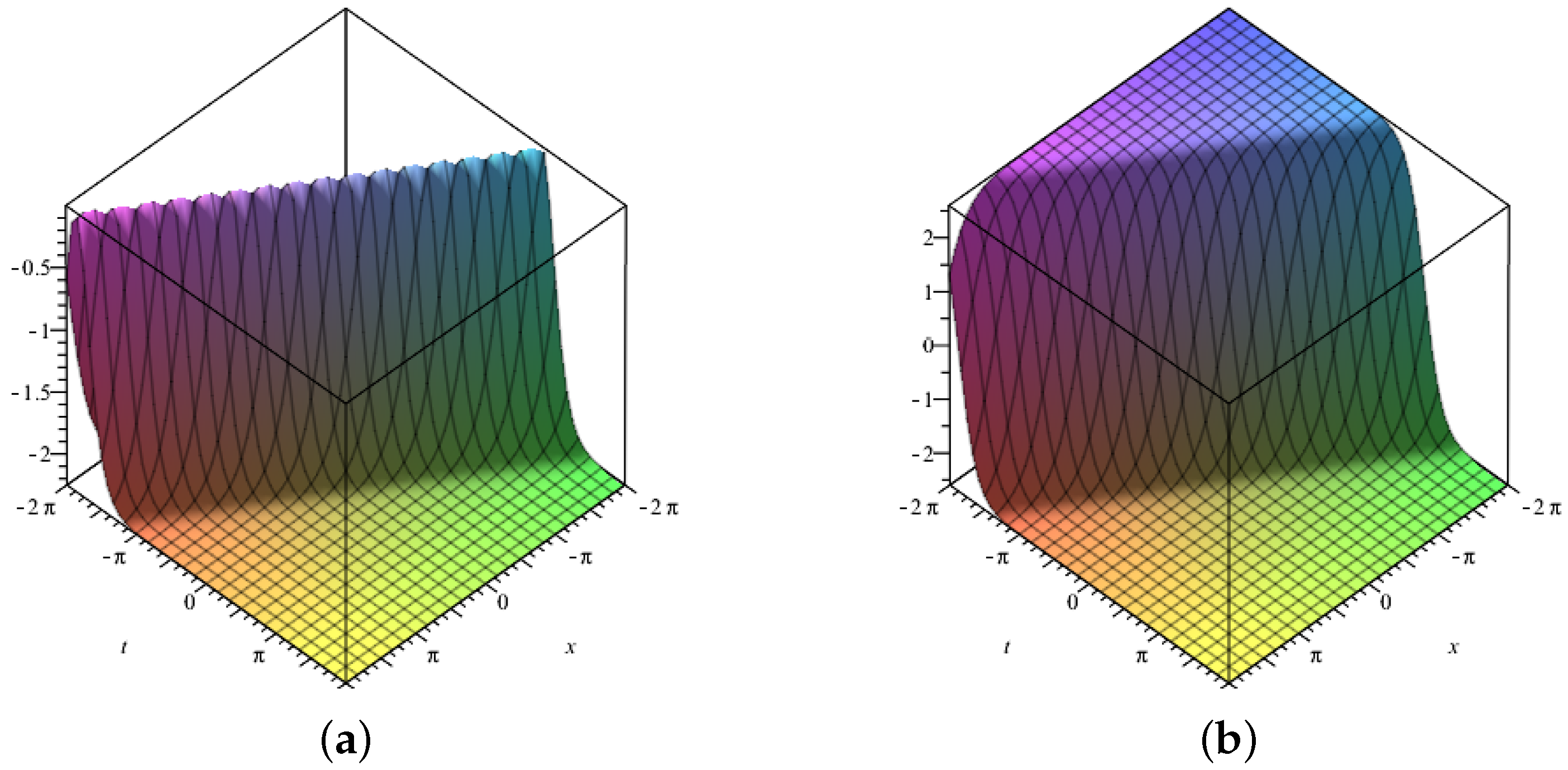
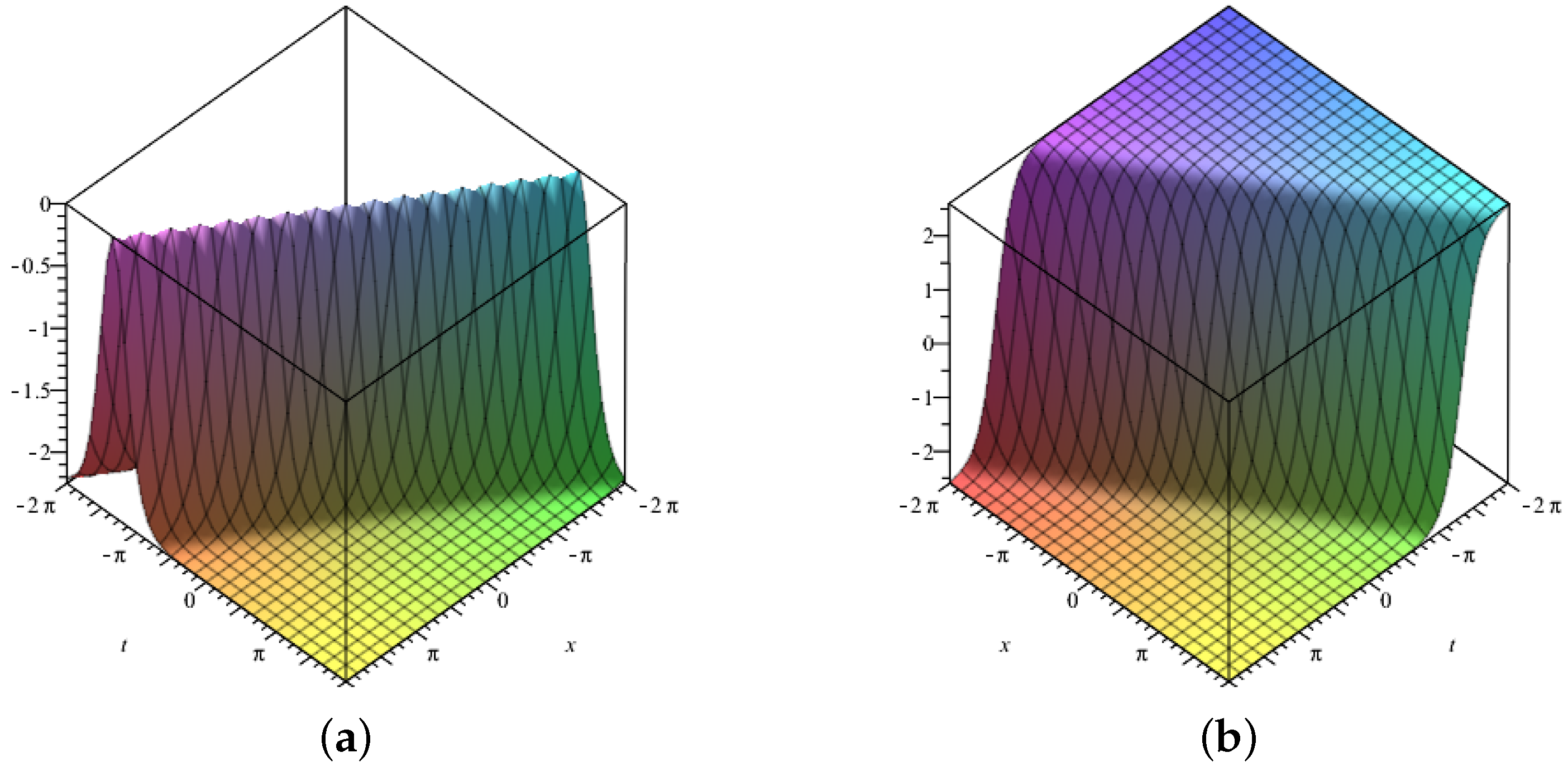
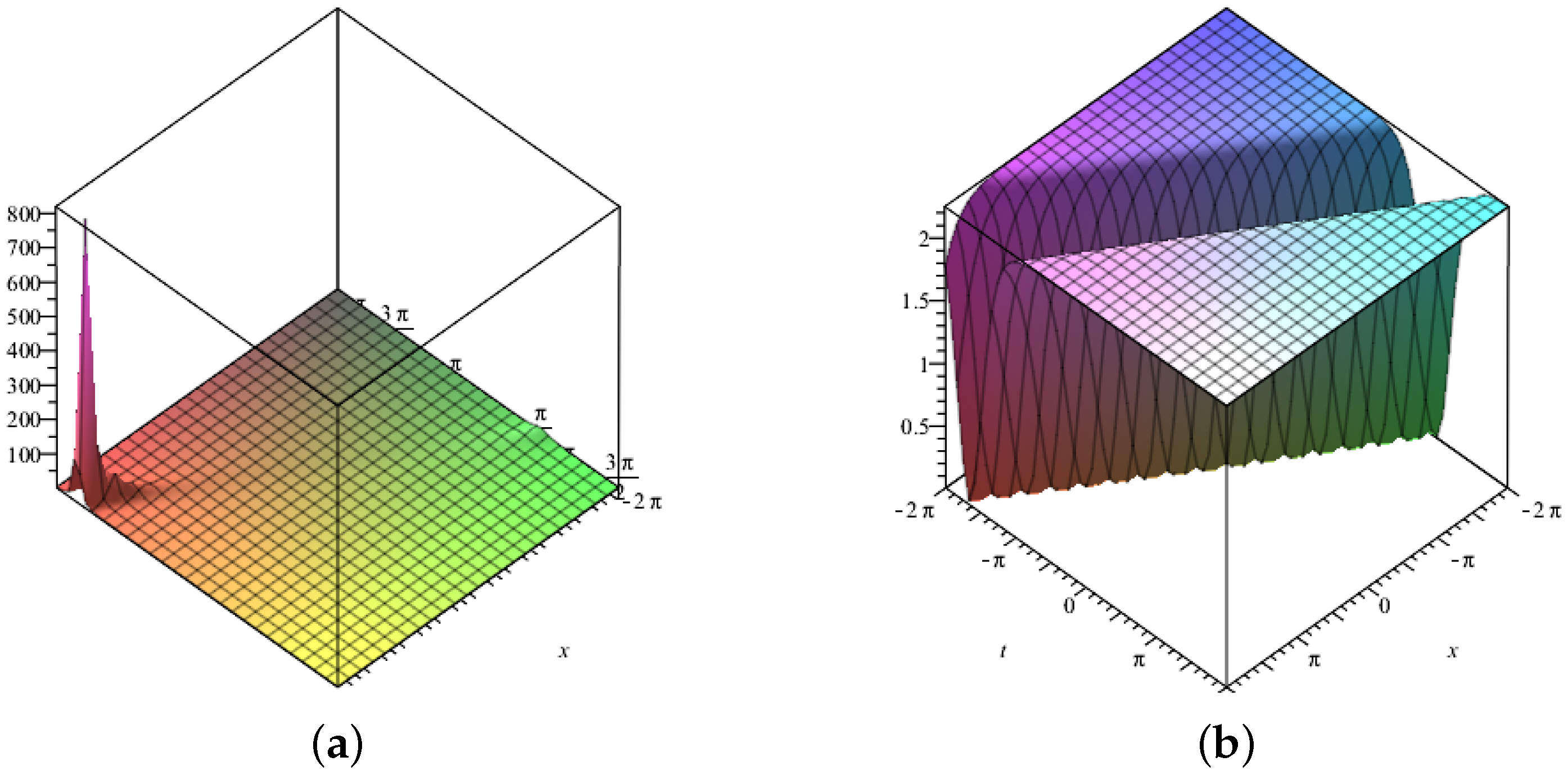
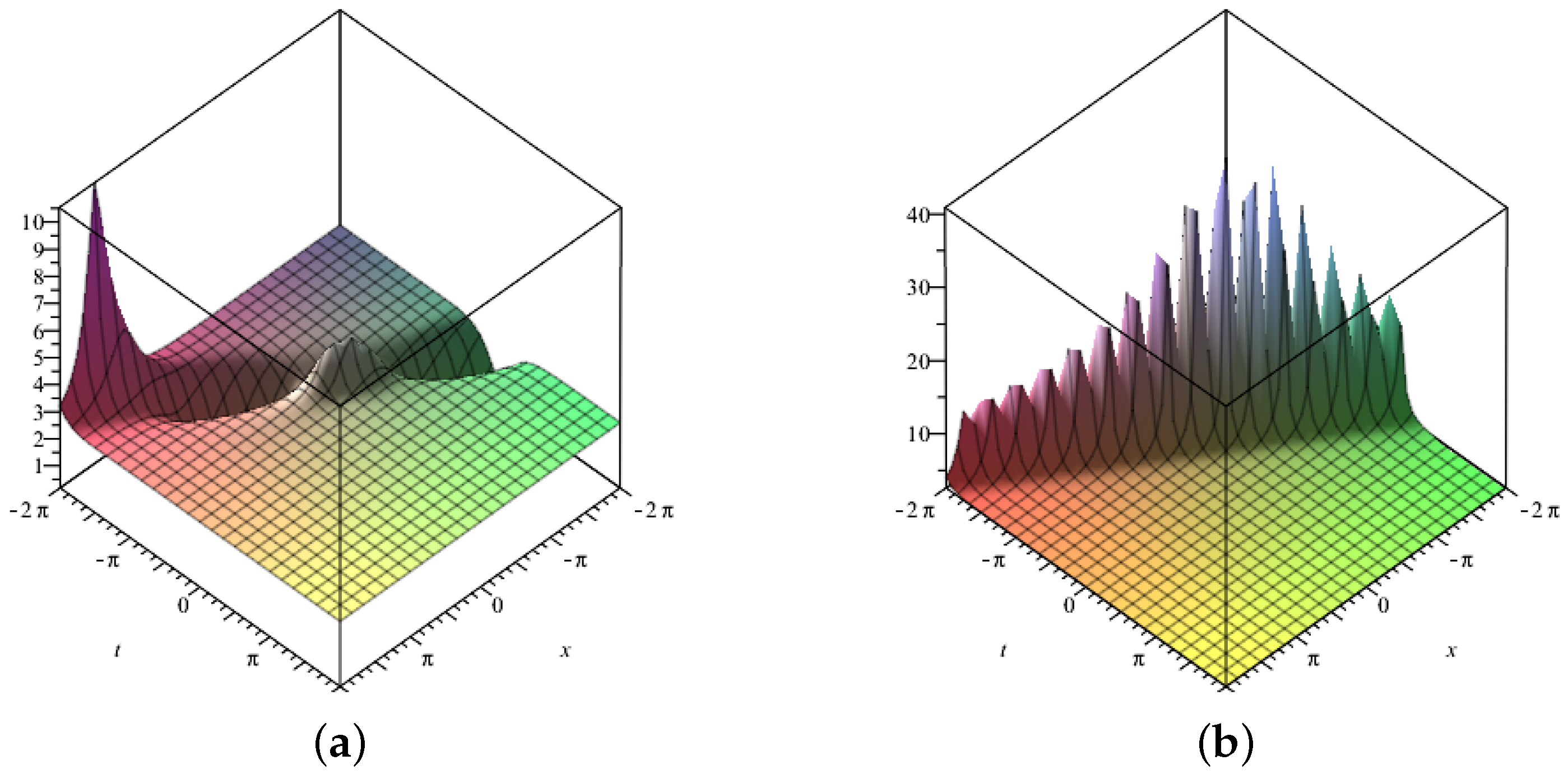
5. Results and Discussions

Three-dimensional surface graphs are used to illustrate the dynamical behavior of the earned results. Each figure consists of two parts, (a) and (b). In Figure 1, Figure 2, Figure 3, Figure 4, Figure 5, Figure 6, Figure 7 and Figure 8, (a) corresponds to fractional value 0.85 while (b) is plotted for 0.99 , respectively. Figure 1, Figure 2, Figure 5, Figure 6 and Figure 9 show traveling variations of solutions in the case of β -fractional derivative, while Figure 3, Figure 4, Figure 7, Figure 8 and Figure 10 show traveling variations of solutions in the case of new local fractional derivative. Figure 1, Figure 2, Figure 3 and Figure 4 show the traveling pattern of solutions U 12 ( x , t ) and V 12 ( x , t ) . It can be noticed that when the value of the fractional parameter approaches 1, the dark soliton behavior dominates in case of U 12 ( x , t ) while dark peakon behavior dominates in case of V 12 ( x , t ) . Figure 5, Figure 6, Figure 7 and Figure 8 show the traveling pattern of solutions U 12 ( x , t ) and V 12 ( x , t ) . It may be noticed that when the value of fractional parameter approaches to 1 the periodic behavior dominates. Kink solitons are observed for U 22 ( x , t ) and V 22 ( x , t ) , as shown in Figure 9 and Figure 10. Part (a) depicts the traveling structure of U 22 ( x , t ) , while (b) represents V 22 ( x , t ) , respectively. The values of free parameters for which these graphs are plotted are mentioned in the caption of each plot. Through graphical illustrations, it can be noticed that various forms of traveling wave structures are obtained for the time fractional nonlinear DSW system using the modified auxiliary equation method including dark, periodic, and kink solitons. Solutions similar to Figure 9 and Figure 10 have already been obtained in the literature [11,15]. Moreover, periodic traveling structure has also been reported for the DSW system [6], which assures the correctness of the MAE method and obtained results. Further, among these obtained structures, dark solitons are shown in Figure 1, Figure 2, Figure 3 and Figure 4. Dark solitons are important in a sense that they are less prone to loss and more stable in disturbing conditions. Dark solitons have thus found extensive use in the fields of nonlinear sciences as they can travel far without any disturbance in their structure.

6. Conclusions

In this paper, the time fractional nonlinear Drinfeld–Sokolov–Wilson system is studied using the modified auxiliary equation method. The definition of β -fractional derivative and a new local fraction derivative is applied to the fractional DSW system. Some of the obtained results are illustrated graphically for thorough understanding of physical behavior of the constructed traveling wave solutions. The variations in the wave structure for various orders of fractional derivative are graphically depicted in Figure 1, Figure 2, Figure 3, Figure 4, Figure 5, Figure 6, Figure 7, Figure 8, Figure 9 and Figure 10. The observed patterns of the fractional DSW system demonstrate that the new local fractional derivative shows more clear traveling structures in comparison to β -fractional derivative, as fractional parameter is taken closer to 1. The obtained solutions show dark soliton, dark peakon, periodic, and kink solitonic structures. They also agree with earlier observations reported in the literature, demonstrating the validity of the suggested method. The work presented also includes some intriguing patterns that can be used in future research on the nature of the DSW system and the results of the aforementioned methodology.

Author Contributions

Conceptualization, G.A. and M.S.; formal analysis, G.A., M.S., I.Z. and M.A.; investigation, G.A., M.S., I.Z., M.A. and A.A.; methodology, G.A., M.S., I.Z., M.A. and A.A.; project administration, G.A., M.S., M.A. and A.A.; software, G.A., M.S. and I.Z.; supervision, G.A. and M.S.; validation, G.A., M.S., M.A. and A.A.; writing—original draft, G.A., M.S., I.Z., M.A. and A.A.; writing—review and editing, G.A., M.S., I.Z., M.A. and A.A. All authors have read and agreed to the published version of the manuscript.

Funding

This research received no external funding.

Institutional Review Board Statement

Not applicable.

Informed Consent Statement

Not applicable.

Data Availability Statement

Not applicable.

Acknowledgments

The authors are also grateful to the anonymous referees for their valuable suggestions, which significantly improved this manuscript.

Conflicts of Interest

The authors declare no conflict of interest.

References

  1. Yang, X.J.; Machado, J.T.; Baleanu, D. Exact traveling-wave solution for local fractional Boussinesq equation in fractal domain. Fractals 2017, 25, 1740006. [Google Scholar] [CrossRef]
  2. Wang, K.J.; Liu, J.H.; Si, J.; Shi, F.; Wang, G.D. N-soliton, breather, lump solutions and diverse traveling wave solutions of the fractional (2 + 1)-dimensional boussinesq equation. Fractals 2023, 31, 2350023. [Google Scholar] [CrossRef]
  3. Fuchs, S. Bijection and Cardinality. In Introduction to Proofs and Proof Strategies; Cambridge University Press: New York, NY, USA, 2023; pp. 155–156. [Google Scholar]
  4. Sprecher, D.A. Elements of Real Analysis; Academic Press, Inc.: New York, NY, USA, 1970; pp. 15–16. [Google Scholar]
  5. Naz, R. Conservation laws for a complexly coupled KdV system, coupled Burgers system and Drinfeld–Sokolov–Wilson system via multiplier approach. Commun. Nonlinear Sci. Numer. Simul. 2010, 15, 1177–1182. [Google Scholar] [CrossRef]
  6. Zhang, W.M. Solitary solutions and singular periodic solutions of the Drinfeld-Sokolov-Wilson equation by variational approach. Appl. Math. Sci. 2011, 5, 1887–1894. [Google Scholar]
  7. Morris, R.; Kara, A. Double reductions/analysis of the Drinfeld–Sokolov–Wilson equation. Appl. Math. Comput. 2013, 219, 6473–6483. [Google Scholar] [CrossRef]
  8. Zhao, Z.; Zhang, Y.; Han, Z. Symmetry analysis and conservation laws of the Drinfeld-Sokolov-Wilson system. Eur. Phys. J. Plus 2014, 129, 1–7. [Google Scholar] [CrossRef]
  9. Jaradat, H.; Al-Shara, S.; Khan, Q.J.; Alquran, M.; Al-Khaled, K. Analytical solution of time-fractional Drinfeld-Sokolov-Wilson system using residual power series method. IAENG Int. J. Appl. Math. 2016, 46, 64–70. [Google Scholar]
  10. Tasbozan, O.; Şenol, M.; Kurt, A.; Özkan, O. New solutions of fractional Drinfeld-Sokolov-Wilson system in shallow water waves. Ocean. Eng. 2018, 161, 62–68. [Google Scholar] [CrossRef]
  11. Singh, J.; Kumar, D.; Baleanu, D.; Rathore, S. An efficient numerical algorithm for the fractional Drinfeld–Sokolov–Wilson equation. Appl. Math. Comput. 2018, 335, 12–24. [Google Scholar] [CrossRef]
  12. Gao, W.; Veeresha, P.; Prakasha, D.; Baskonus, H.M.; Yel, G. A powerful approach for fractional Drinfeld–Sokolov–Wilson equation with Mittag-Leffler law. Alex. Eng. J. 2019, 58, 1301–1311. [Google Scholar] [CrossRef]
  13. Srivastava, H.; Saad, K.M. Some new and modified fractional analysis of the time-fractional Drinfeld–Sokolov–Wilson system. Chaos Interdiscip. J. Nonlinear Sci. 2020, 30, 113104. [Google Scholar] [CrossRef] [PubMed]
  14. Al-Rozbayani, A.M.; Ali, A.H. Applied Sumudu transform with Adomian decomposition method to the coupled Drinfeld–Sokolov–Wilson system. AL-Rafidain J. Comput. Sci. Math. 2021, 15, 139–147. [Google Scholar] [CrossRef]
  15. Saifullah, S.; Ali, A.; Shah, K.; Promsakon, C. Investigation of fractal fractional nonlinear Drinfeld–Sokolov–Wilson system with non-singular operators. Results Phys. 2022, 33, 105145. [Google Scholar] [CrossRef]
  16. Wang, K.J.; Wang, G.D. Periodic solution of the (2+ 1)-dimensional nonlinear electrical transmission line equation via variational method. Results Phys. 2021, 20, 103666. [Google Scholar] [CrossRef]
  17. Hussain, R.; Imtiaz, A.; Rasool, T.; Rezazadeh, H.; İnç, M. Novel exact and solitary solutions of conformable Klein–Gordon equation via Sardar-subequation method. J. Ocean. Eng. Sci. 2022. [Google Scholar] [CrossRef]
  18. Wang, K.J.; Si, J.; Wang, G.D.; Shi, F. A new fractal modified Benjamin-Bona-Mahony equation: Its generalized variational principle and abundant exact solutions. Fractals 2023, 31, 2350047. [Google Scholar] [CrossRef]
  19. Wang, K.J.; Liu, J.H. Diverse optical solitons to the nonlinear Schrödinger equation via two novel techniques. Eur. Phys. J. Plus 2023, 138, 1–9. [Google Scholar] [CrossRef]
  20. Atangana, A.; Baleanu, D.; Alsaedi, A. Analysis of time-fractional Hunter-Saxton equation: A model of neumatic liquid crystal. Open Phys. 2016, 14, 145–149. [Google Scholar] [CrossRef]
  21. Atangana, A.; Goufo, E.F.D. Extension of Matched Asymptotic Method to Fractional Boundary Layers Problems. Math. Probl. Eng. 2014, 2014, 107535. [Google Scholar] [CrossRef]
  22. Guzman, P.; Langton, G.; Lugo, L.; Medina, J.; Valdés, J. A new definition of a fractional derivative of local type. J. Math. Anal. 2018, 9, 88–98. [Google Scholar]
  23. Martínez, H.; Rezazadeh, H.; Inc, M.; Akinlar, M. New solutions to the fractional perturbed Chen-Lee-Liu equation with a new local fractional derivative. In Waves in Random and Complex Media; Taylor & Francis: Abingdon, UK, 2021; pp. 1–36. [Google Scholar]
  24. Akram, G.; Sadaf, M.; Atta Ullah Khan, M. Soliton solutions of the resonant nonlinear Schrödinger equation using modified auxiliary equation method with three different nonlinearities. Math. Comput. Simul. 2023, 206, 1–20. [Google Scholar] [CrossRef]
  25. Akram, G.; Sadaf, M.; Zainab, I. The dynamical study of Biswas-Arshed equation via modified auxiliary equation method. Optik- Int. J. Light Electron Opt. 2022, 255, 168614. [Google Scholar] [CrossRef]
  26. Akram, G.; Sadaf, M.; Zainab, I. Observations of fractional effects of β-derivative and M-truncated derivative for space time fractional Phi-4 equation via two analytical techniques. Chaos Solitons Fractals 2022, 154, 111645. [Google Scholar] [CrossRef]
Figure 1. Three–dimensional graphics corresponding to β –fractional derivative of (a) | U 22 ( x , t ) | with β = 0.85 , α = 1 , r = 1 , s = 0.5 , η = 1 , η 0 = 0.5 , η 1 = 2 , η 2 = 0.5 (b) | V 22 ( x , t ) | with β = 0.99 , α = 1 , r = 1 , s = 0.5 , η = 1 , η 0 = 0.5 , η 1 = 2 , η 2 = 0.5 .
Fractalfract 07 00665 g001
Figure 2. Three–dimensional graphics corresponding to a new local fractional derivative of (a) | U 22 ( x , t ) | with β = 0.85 , α = 1 , r = 1 , s = 0.5 , η = 1 , η 0 = 0.5 , η 1 = 2 , η 2 = 0.5 (b) | V 22 ( x , t ) | with β = 0.99 , α = 1 , r = 1 , s = 0.5 , η = 1 , η 0 = 0.5 , η 1 = 2 , η 2 = 0.5 .
Fractalfract 07 00665 g002
Figure 3. Three–dimensional graphics corresponding to β –fractional derivative of (a) | U 12 ( x , t ) | with β = 0.85 , α = 1 , r = 1 , s = 0.5 , η = 1 , η 0 = 0.5 , η 1 = 2 , η 2 = 0.5 (b) | U 12 ( x , t ) | with β = 0.99 , α = 1 , r = 1 , s = 0.5 , η = 1 , η 0 = 0.5 , η 1 = 2 , η 2 = 0.5 .
Fractalfract 07 00665 g003
Figure 4. Three–dimensional graphics corresponding to β –fractional derivative of (a) | V 12 ( x , t ) | with β = 0.85 , α = 1 , r = 1 , s = 0.5 , η = 1 , η 0 = 0.5 , η 1 = 2 , η 2 = 0.5 (b) | V 12 ( x , t ) | with β = 0.99 , α = 1 , r = 1 , s = 0.5 , η = 1 , η 0 = 0.5 , η 1 = 2 , η 2 = 0.5 .
Fractalfract 07 00665 g004
Figure 5. Three–dimensional graphics corresponding to a new local fractional derivative of (a) | U 12 ( x , t ) | with β = 0.85 , α = 1 , r = 1 , s = 0.5 , η = 1 , η 0 = 0.5 , η 1 = 2 , η 2 = 0.5 (b) | U 12 ( x , t ) | with β = 0.99 , α = 1 , r = 1 , s = 0.5 , η = 1 , η 0 = 0.5 , η 1 = 2 , η 2 = 0.5 .
Fractalfract 07 00665 g005
Figure 6. Three–dimensional graphics corresponding to a new local fractional derivative of (a) | V 12 ( x , t ) | with β = 0.85 , α = 1 , r = 1 , s = 0.5 , η = 1 , η 0 = 0.5 , η 1 = 2 , η 2 = 0.5 (b) | V 12 ( x , t ) | with β = 0.99 , α = 1 , r = 1 , s = 0.5 , η = 1 , η 0 = 0.5 , η 1 = 2 , η 2 = 0.5 .
Fractalfract 07 00665 g006
Figure 7. Three-dimensional graphics corresponding to β -fractional derivative of (a) | U 12 ( x , t ) | with β = 0.85 , α = 1 , r = 1 , s = 0.5 , η = 1 , η 0 = 0.5 , η 1 = 2 , η 2 = 0.5 (b) | U 12 ( x , t ) | with β = 0.99 , α = 1 , r = 1 , s = 0.5 , η = 1 , η 0 = 0.5 , η 1 = 2 , η 2 = 0.5 .
Fractalfract 07 00665 g007
Figure 8. Three–dimensional graphics corresponding to β –fractional derivative of (a) | V 12 ( x , t ) | with β = 0.85 , α = 1 , r = 1 , s = 0.5 , η = 1 , η 0 = 0.5 , η 1 = 2 , η 2 = 0.5 (b) | V 12 ( x , t ) | with β = 0.99 , α = 1 , r = 1 , s = 0.5 , η = 1 , η 0 = 0.5 , η 1 = 2 , η 2 = 0.5 .
Fractalfract 07 00665 g008
Figure 9. Three–dimensional graphics corresponding to a new local fractional derivative of (a) | U 12 ( x , t ) | with β = 0.85 , α = 1 , r = 1 , s = 0.5 , η = 1 , η 0 = 0.5 , η 1 = 2 , η 2 = 0.5 (b) | U 12 ( x , t ) | with β = 0.99 , α = 1 , r = 1 , s = 0.5 , η = 1 , η 0 = 0.5 , η 1 = 2 , η 2 = 0.5 .
Fractalfract 07 00665 g009
Figure 10. Three–dimensional graphics corresponding to a new local fractional derivative of (a) | V 12 ( x , t ) | with β = 0.85 , α = 1 , r = 1 , s = 0.5 , η = 1 , η 0 = 0.5 , η 1 = 2 , η 2 = 0.5 (b) | V 12 ( x , t ) | with β = 0.99 , α = 1 , r = 1 , s = 0.5 , η = 1 , η 0 = 0.5 , η 1 = 2 , η 2 = 0.5 .
Fractalfract 07 00665 g010
Disclaimer/Publisher’s Note: The statements, opinions and data contained in all publications are solely those of the individual author(s) and contributor(s) and not of MDPI and/or the editor(s). MDPI and/or the editor(s) disclaim responsibility for any injury to people or property resulting from any ideas, methods, instructions or products referred to in the content.

