Article

Mathematical Analysis of Fractal-Fractional Mathematical Model of COVID-19

by
Muhammad Sinan
1,* and
Nadiyah Hussain Alharthi
2
1
School of Mathematical Sciences, University of Electronic Science and Technology of China, Chengdu 611731, China
2
Department of Mathematics and Statistics, College of Science Imam Mohammad Ibn Saud Islamic University, P.O. Box 90950, Riyadh 11623, Saudi Arabia
*
Author to whom correspondence should be addressed.
Fractal Fract. 2023, 7(5), 358; https://doi.org/10.3390/fractalfract7050358
Submission received: 20 March 2023 / Revised: 24 April 2023 / Accepted: 24 April 2023 / Published: 27 April 2023

Abstract

:
In this work, we modified a dynamical system that addresses COVID-19 infection under a fractal-fractional-order derivative. The model investigates the psychological effects of the disease on humans. We establish global and local stability results for the model under the aforementioned derivative. Additionally, we compute the fundamental reproduction number, which helps predict the transmission of the disease in the community. Using the Carlos Castillo-Chavez method, we derive some adequate results about the bifurcation analysis of the proposed model. We also investigate sensitivity analysis to the given model using the criteria of Chitnis and his co-authors. Furthermore, we formulate the characterization of optimal control strategies by utilizing Pontryagin’s maximum principle. We simulate the model for different fractal-fractional orders subject to various parameter values using Adam Bashforth’s numerical method. All numerical findings are presented graphically.

1. Introduction

Recently, the new coronavirus has become a severe global issue that is wreaking havoc on the global economy and the health of people. Human society, endowed with modern technology, has been currently infected with the COVID-19 disease, which is a dreadful infection that has mostly harmed underdeveloped countries more than developed countries. According to reports, the world’s first case of the new coronavirus was reported at the end of 2019. The study of infectious diseases is crucial to investigate the spread of various diseases in communities, and researchers have investigated the effect of these infectious diseases on the behavior of living organisms. It is worth noting that infectious diseases have affected humans, as well as other animals and plants, very badly for many centuries. For instance, see [1]. The pandemic has not only affected the world’s economy but also caused the loss of human lives. The main source of COVID-19 infection is droplets from the afflicted person’s mouth or nose when speaking or sneezing, and people who are in close proximity to the afflicted person are at risk of contracting the sickness. Almost every government in the world has embraced the lockdown policy as a preventive measure to safeguard the safety of its population, and in such cases, doctors and paramedics have pledged to provide health services to those who have been affected. Since the beginning of the COVID-19 pandemic, many researchers in their respective fields have studied coronavirus infection and attempted to identify possible ways to immunize humans against this virus in order to follow the World Health Organization’s (WHO) rules and regulations and immunize people to the maximum extent.
Since the onset of the COVID-19 pandemic, numerous scholars across various disciplines have conducted research on coronavirus infection. Determining the apex of infection within a particular country can inform decisions on how to mitigate these occurrences and the probability of future outbreaks with fewer infected individuals. The World Health Organization (WHO) has established guidelines and protocols to optimize the immunization of individuals. This investigation endeavors to identify individual perspectives on adhering to stay-at-home orders during the COVID-19 pandemic through the use of metaphors, and explores the correlation between these perspectives, stress, depression, and anxiety. It is important to acknowledge that measures taken to contain the spread of the pandemic may also result in diverse psychological complications.
A novel mathematical model has been created and analyzed to evaluate the interplay between COVID-19, Zika, chikungunya, and dengue co-dynamics. The aim is to determine the influence of COVID-19 on the dynamics of Zika, dengue, and chikungunya, as well as the reverse effect [2]. A proposed SEQAIHR model with saturated treatment is presented, and the biological feasibility of the model solutions is assessed, along with the calculation of the basic reproduction number (R0). The model displays transcritical, backward bifurcation, and forward bifurcation with hysteresis under certain restrictions with respect to different parameters. To validate the model, it is fitted with actual COVID-19 infection data from Hong Kong between December 19th, 2021 and April 3rd, 2022, and the model parameters are estimated. Sensitivity analysis is conducted to identify the most sensitive parameters that affect R0. R0 is estimated using actual initial growth data of COVID-19, and the effective reproduction number is calculated for the same period. Finally, an optimal control problem is proposed, taking into account effective vaccination and saturated treatment for the hospitalized class, to reduce the density of the infected class and minimize the implemented cost [3].
Quantitative data were analyzed using the Kruskal–Wallis test, while qualitative data was subjected to content analysis. The findings indicated that a significant proportion of the participants perceived staying at home as a state of confinement, ennui/dejection, and powerlessness. Conversely, some participants regarded staying at home as a conscientious act, a chance, and a prerequisite for ensuring safety. Participants who viewed staying at home as a form of confinement or a cause of ennui/dejection exhibited more psychological challenges, whereas those who perceived it as a responsibility or an opportunity experienced fewer difficulties.
Since its inception as a subject over a century ago, mathematical modeling and investigation of infectious diseases have been central to the study of infectious disease transmission. With the advancement of better processing, data software, and the availability of potential for transmitting and preserving information over the internet, electronic surveillance of infectious diseases has become common. Anderson et al. [4] found that mathematical models have been used as powerful tools for investigating epidemiological features of various diseases. Researchers have subsequently proposed appropriate control and preventative techniques to better understand infectious illnesses. Infectious illnesses and their transmission have been heavily influenced by human behavior and societal responses. Control efforts have been implemented to better understand the effects of human behavior and societal responses on the spread of infectious illnesses. The general population reacted to avian influenza in behavioral, psychological, and societal ways. Individuals’ psychological reactions throughout the epidemic affected the pace with which it spread, as well as the potential for emotional and societal difficulties.
In this paper, we develop a COVID-19 epidemic model that includes a nonlinear incidence rate for the spread of the COVID-19 virus from infective humans to susceptible humans, which accounts for the population saturation effect. Additionally, we consider a non-monotone incidence rate for the spread of the COVID-19 virus from infective humans to susceptible humans, which captures the psychological effect within humans.
Fractal-fractional calculus has gained much popularity in recent times. In this branch, the word ‘fractal derivative,’ also called the Hausdorff derivative, is a non-Newtonian generalization of the traditional order derivative. This derivative deals with the measurement of fractals, which are concepts defined in fractal geometry. The concept was introduced when the classical derivative failed to explain the anomalous behavior of the diffusion process in the fractal nature of the media. This derivative is local in nature compared to the ordinary fractional order derivative, which is non-local. It is worth noting that certain phenomena related to porous media, turbulence, aquifers, and other media usually display fractal properties. The use of the fractal-fractional derivative has become increasingly popular in recent years due to its ability to model complex systems with high accuracy. This type of derivative takes into account the fractal nature of many natural phenomena, such as the branching patterns of trees or the irregular shapes of coastlines. By incorporating fractal geometry into the traditional calculus framework, the fractal-fractional derivative provides a more comprehensive understanding of the behavior of complex systems. This has important applications in fields such as physics, engineering, and finance, where accurate modeling of complex systems is crucial. Additionally, the use of the fractal-fractional derivative has the potential to lead to new insights and discoveries in these fields, making it an exciting area of research.
The mentioned form of the derivative has been used effectively in recent years to investigate various real-world problems. For some recent work, we refer to [5,6,7,8,9,10,11]. Therefore, keeping this in mind, we also investigate our proposed model in terms of the Caputo fractal-fractional order derivative. We establish a detailed analysis, including the construction of basic reproductive numbers, and global and local stability analysis using various approaches. We also use mathematical arguments to develop sufficient conditions for bifurcation and sensitivity analysis for the proposed model. Finally, we present various numerical simulations using the Adam Bashforth method, and all the results are displayed graphically.
The manuscript is structured as follows: In Section 2, we present fundamental definitions and theorems that underpin this study. In Section 3, we determine the disease-free and endemic equilibrium points and calculate the basic reproduction number at the disease-free equilibrium point. Additionally, we conduct a stability analysis based on the equilibrium point. In Section 4, we compute the saddle node resulting from the zero eigenvalue and derive several outcomes concerning bifurcation analysis. In Section 5, we perform sensitivity analysis based on the basic reproduction number R 0 . In Section 6, we apply vaccination and treatment control variables to prevent the population from contracting the COVID-19 virus again. In Section 7, we establish the numerical scheme for the fractal-fractional problem from [12] for the numerical simulation of the COVID-19 model. The numerical values and initial conditions to the compartments/classes with descriptions are given in Table 1 and Table 2. Finally, we present the outcomes and discussion and summarize the numerical simulations and the paper in Section 8 and Section 9, respectively.

2. Preliminaries

In this section, we recall fractional-fractional operators such that:
Theorem 1
([9]). Assume that the function s ( t ) is differentiable in the open interval ( a , b ) . Then, the fractal-fractional derivative of s of order λ in the Caputo sense with power law is given as:
a FFP D t κ , λ s ( t ) = 1 Γ [ m λ ] a t d s ( ξ ) d ξ κ ( t ξ ) m λ 1 d ξ , m 1 < λ m , 0 < m 1 < κ m d s ( ξ ) d ξ κ = lim t ξ s ( t ) s ( ξ ) t κ ξ κ .
 if s is fractal differentiable on ( a , b ) with order κ.
Theorem 2
([9]). The fractal-fractional integral of function s with fractal order κ > 0 and fractional order α > 0 is defined as:
0 FFP I t κ , λ s ( t ) = κ Γ ( λ ) 0 t ξ λ 1 s ( ξ ) ( t ξ ) λ 1 d ξ .
 if s ( t ) is continuous in an opened interval [ a , b ] .
Definition 1.
Suppose we consider the fractal-fractional non-linear ODE such that
0 FFP D κ , λ u ( t ) = v ( t , u ( t ) ) , w i t h u ( 0 ) = u 0 .
From Zhang et al. [12] the resultant numerical scheme for the Equation (3) can be written as:
u ( k + 1 ) = u ( 0 ) + κ λ Γ ( λ + 2 ) p = 0 m t ( p ) κ 1 v u ( p ) , t p × ( m + 1 p ) κ ( m p + 2 + κ ) ( m p ) κ ( m p + 2 + 2 κ ) t ( p 1 ) κ 1 v u ( p 1 ) , t ( p 1 ) ( m + 1 p ) κ + 1 ( m p ) κ ( m p + 1 + κ ) .

Formulation of the Proposed Model of COVID-19

The model is modified from the existence SIQR model of [16]:
d S d t = Λ μ S β S I N , d I d t = β S I N ( μ + γ + δ + α ) I , d Q d t = δ I ( μ + ϵ + α ) Q , d R d t = γ I + ϵ Q μ R .
The modified version of the model (5) is as follows in the fractal-fractional Caputo sense with power law kernel:
0 FFP D κ , λ S ( t ) = υ τ S ( t ) ϑ S ( t ) I ( t ) 1 + ω I ( t ) , 0 FFP D κ , λ I ( t ) = ϑ S ( t ) I ( t ) 1 + ω I ( t ) ( τ + χ + ν + ϱ 1 ) I ( t ) , 0 FFP D κ , λ Q ( t ) = ν I ( t ) ( τ + ϖ + ϱ 2 ) Q ( t ) , 0 FFP D κ , λ P ( t ) = χ I ( t ) + ϖ Q ( t ) τ P ( t ) , 0 FFP D κ , λ D I Q = ϱ 1 I ( t ) + ϱ 2 Q ( t ) .
where the parameters are defined as: υ = recruitment rate, τ natural death rate, ϑ transmission rate, ω psychological effect on humans [14,17], ϱ 1 , ϱ 2 death rates of infected and quarantine population due to disease, respectively, χ , ϖ are recovery rates of infected and quarantine population, respectively, and ν is the rate of infection. The functions or classes are defined as: S ( t ) is the susceptible human population, I ( t ) is the infected human population, Q ( t ) is the quarantine population, P ( t ) is the protected population, and D I Q represents deaths in infected and quarantine populations.

3. Equilibrium Points and Stability

Here we derive our main results in the following sub-sections.

3.1. Equilibrium Points

We have two types of equilibrium points such as disease-free and endemic equilibrium points. In the disease-free equilibrium point, we have no infection in the population. Thus in the mathematical model the infected compartments become zero while in endemic equilibrium the model counts as a whole. We denote the disease-free equilibrium point by E 0 while the disease-endemic equilibrium point is denoted by E * . The equilibrium points are as follows:
E 0 = ν τ , 0 , 0 , 0 , 0 .
while the disease-endemic equilibrium is computed in terms of one class, such that
E * = S * , I * , Q * , P * , D * ,
where
S * = ν ( 1 + ω I * ) ( 1 + ω I * ) + ϑ I * , Q * = ϱ 1 ϱ 2 I * , P * = 1 τ χ τ ϖ ϱ 2 ϱ 1 I * .

3.2. Basic Reproduction Number

Here we are going to compute the fundamental reproduction number as
d Z d t E 0 = f v .
where the non-linear and linear terms from the infected classes in matrix f and v , respectively are given as
f = ϑ S ( t ) I ( t ) 1 + ω I ( t ) 0 , v = ( τ + χ + ν + ϱ 1 ) I ( t ) ( τ + ϖ + ϱ 2 ) Q ( t ) ν I ( t ) .
Now, the Jacobian matrix of f and v is given by
F = ϑ S 0 ( t ) I 0 ( t ) 1 + ω I 0 ( t ) ϑ S 0 ( t ) I 0 ( t ) ω ϑ ( 1 + ω I 0 ( t ) ) 2 0 0 0 , and V = τ + χ + ν + ϱ 1 0 ν τ + ϖ + ϱ 2 .
We now calculate the inverse of matrix V and the next generation matrix G ( E 0 ) , such that
V 1 = 1 τ + χ + ν + ϱ 1 0 ν ( ϱ 1 + τ + ϖ ) ( τ + χ + ν + ϱ 1 ) 1 ϱ 2 + τ + ϖ , and G ( E 0 ) = ϑ S 0 ( τ + χ + ν + ϱ 1 ) 0 0 0 .
Thus, the non-zero and largest eigenvalue is the basic reproduction number R 0 is
R 0 = ϑ S 0 ( τ + χ + ν + ϱ 1 ) ,
where S 0 = υ τ .

3.3. Stability Analysis

Let a fractal-fractional order linear homogenous system of the following form be given:
0 FFP D t κ , λ s ( t ) = A s ( t ) , s ( 0 ) = s 0 .
where A N n × n ( R ) & 0 < κ , λ 1 . The following theorems are on the stability of a linear homogenous system (15).
Theorem 3.
The COVID-19 model at the disease-free equilibrium point E 0 is locally asymptotically stable if R 0 < 1 , otherwise unstable.
Proof. 
The Jacobian matrix of the system (6) at disease-free equilibrium point E 0 is given by
J E 0 = τ ϑ S 0 0 0 0 0 ϑ S 0 ( ϱ 1 + ν + τ + χ ) 0 0 0 0 υ ( ϱ 2 + τ + ϖ ) 0 0 0 χ ϖ τ 0 0 ϱ 1 ϱ 2 0 0 .
The two eigenvalues are ζ 1 = ζ 2 = τ . The reduced matrix becomes
J E 0 = ϑ S 0 ( ϱ 1 + ν + τ + χ ) 0 0 υ ( ϱ 2 + τ + ϖ ) 0 ϱ 1 ϱ 2 0 .
The characteristic equation becomes
ζ ( ζ 2 + α 1 ζ + α 2 ) = 0 .
Thus, the roots of the characteristic Equation (18) are given by
ζ 1 = ( ϱ 1 + ν + τ + χ ) ( 1 R 0 ) , ζ 2 = ( ϱ 2 + τ + ϖ ) , ζ 3 = 0 .
We have a single zero eigenvalue while according to the eigenvalues the system is locally asymptotically stable. For the zero eigenvalue, we proceed with the saddle-node bifurcation in the next section. For this, we take basic reproduction number R 0 equal to 1 such that
R 0 = ϑ S 0 ( τ + χ + ν + ϱ 1 ) = 1 .
From Equation (20), we have the parameter ϑ 0 = ϑ , that is
ϑ 0 = τ ( τ + χ + ν + ϱ 1 ) ν .
Thus, Equation (21) is the bifurcation parameter. □

4. Bifurcation Analysis

In this section, we demonstrate bifurcation analysis of the system (6). We follow theorem A of Carlos Castillo-Chavez and Song [18] and Buonomo and Lacitignola [19], which is discussed above to obtain the required result. Recall the system (6):
0 FFP D κ , λ S ( t ) = υ τ S ( t ) ϑ S ( t ) I ( t ) 1 + ω I ( t ) , 0 FFP D κ , λ I ( t ) = ϑ S ( t ) I ( t ) 1 + ω I ( t ) ( τ + χ + ν + ϱ 1 ) I ( t ) , 0 FFP D κ , λ Q ( t ) = ν I ( t ) ( τ + ϖ + ϱ 2 ) Q ( t ) , 0 FFP D κ , λ P ( t ) = χ I ( t ) + ϖ Q ( t ) τ P ( t ) , 0 FFP D κ , λ D I Q = ϱ 1 I ( t ) + ϱ 2 Q ( t ) .
Now, put S ( t ) = u 1 , I ( t ) = u 2 , Q ( t ) = u 3 , P ( t ) = u 4 , & D I Q ( t ) = u 5 , while the right hand side equals g k for k = 1 , 2 , 3 , 4 , 5 . Thus the system (22) becomes
g 1 = υ τ u 1 ϑ u 1 u 2 1 + ω u 2 , g 2 = ϑ u 1 u 2 1 + ω u 2 ( τ + χ + ν + ϱ 1 ) u 2 , g 3 = ν u 2 ( τ + ϖ + ϱ 2 ) u 3 , g 4 = χ u 2 + ϖ u 3 τ u 4 , g 5 = ϱ 1 u 2 + ϱ 2 u 3 .
Theorem 4.
By applying Theorem A we show that system (6) can exhibit a forward bifurcation, when ϑ = ϑ 0 .
Proof. 
According to Equation (20), the disease-free equilibrium E 0 exhibits a single zero eigenvalue, while the remaining eigenvalues are either real or possess negative real components. Consequently, when ϑ = ϑ 0 (or R 0 = 1 ), E 0 represents a non-hyperbolic equilibrium, thereby satisfying assumption (A1) of Theorem A. Let w = w 1 , w 2 , w 3 , w 4 , w 5 T denote a right eigenvector linked to the zero eigenvalue ζ 3 = 0 . It follows that
τ w 1 ϑ w 2 ν τ [ ϑ ν τ ( ϱ 1 + ν + τ + χ ) ] w 2 ν w 2 ( ϱ 2 + τ + ϖ ) w 2 χ w 2 + ϖ w 3 τ w 4 ϱ 1 w 2 + ϱ 2 w 3 = 0 0 0 0 0 .
Thus, the non-zero ws are given as
w 1 = ϑ w 3 S 0 τ ϱ 1 , w 2 = ϱ 2 w 3 ϱ 1 , and w 4 = ϖ χ ϱ 2 τ w 3 .
Furthermore, the left eigenvector v = v 1 , v 2 , v 3 , v 4 , v 5 satisfying v · w = 1 is given by:
τ v 1 [ ϑ S 0 ( ϱ 1 + ν + τ + χ ) ] v 2 ϑ S 0 v 1 + ν v 3 + χ v 4 + ϱ 1 v 5 ϖ v 4 ( ϱ 2 + τ + ϖ ) v 3 + ϱ 2 v 5 τ v 4 0 = 0 0 0 0 0 .
Thus, the non-zero vs are given as
v 2 = v 3 [ ν + ϱ 2 ϱ 1 ( ϱ 2 + τ + ϖ ) ] ( ϱ 1 + ν + τ + χ ) ϑ S 0 , v 5 = v 3 ϱ 2 + τ + ϖ ϱ 2 .
The coefficients a and b defined in Theorem A are given by
a = k , i , j = 1 5 v k w i w j 2 g k u i u j E 0 , ϑ 0 , b = k , i = 1 5 v k w i 2 g k u i ϑ E 0 , ϑ 0 .
Now, from Equations (23), (25), (27) and (28) we have
a = v 2 w 1 2 2 g 2 u 1 2 E 0 , ϑ 0 + v 2 w 1 w 2 2 g 2 u 1 u 2 E 0 , ϑ 0 + v 2 w 1 w 3 2 g 2 u 1 u 3 E 0 , ϑ 0 + v 2 w 1 w 4 2 g 2 u 1 u 4 E 0 , ϑ 0 + v 3 w 2 w 1 2 g 3 u 2 u 1 E 0 , ϑ 0 + v 3 w 2 2 2 g 3 u 2 2 E 0 , ϑ 0 + v 3 w 2 w 3 2 g 3 u 2 u 3 E 0 , ϑ 0 + v 3 w 2 w 4 2 g 3 u 2 u 4 E 0 , ϑ 0 + v 5 w 3 w 1 2 g 5 u 5 u 1 E 0 , ϑ 0 + v 5 w 3 w 2 2 g 5 u 5 u 2 E 0 , ϑ 0 + v 5 w 3 w 3 2 g 5 u 5 u 3 E 0 , ϑ 0 + v 5 w 3 w 4 2 g 5 u 5 u 4 E 0 , ϑ 0 ,
which yields that
a = v 3 τ ϱ 2 w 3 ( τ + χ + ν + ϱ 1 ) ϱ 1 2 ν + ϱ 2 ϱ 1 ( ϱ 2 + τ + ϖ ) ( ϱ 1 + ν + τ + χ ) ϑ ν τ ,
and b is given as
b = v 2 w 1 2 g 2 u 1 ϑ E 0 , ϑ 0 + v 2 w 2 2 g 2 u 2 ϑ E 0 , ϑ 0 + v 2 w 3 2 g 2 u 3 ϑ E 0 , ϑ 0 + v 2 w 4 2 g 2 u 4 ϑ E 0 , ϑ 0 + v 3 w 1 2 g 3 u 1 ϑ E 0 , ϑ 0 + v 3 w 2 2 g 3 u 2 ϑ E 0 , ϑ 0 + v 3 w 3 2 g 3 u 3 ϑ E 0 , ϑ 0 + v 3 w 4 2 g 3 u 4 ϑ E 0 , ϑ 0 + v 5 w 1 2 g 5 u 1 ϑ E 0 , ϑ 0 + v 5 w 2 2 g 5 u 2 ϑ E 0 , ϑ 0 + v 5 w 2 2 g 5 u 2 ϑ E 0 , ϑ 0 + v 5 w 3 2 g 5 u 3 ϑ E 0 , ϑ 0 + v 5 w 4 2 g 5 u 4 ϑ E 0 , ϑ 0 .
After evaluation of b, such that
b = ϱ 2 v 3 w 3 ν + ϱ 2 ϱ 1 ( ϱ 2 + τ + ϖ ) ϱ 1 ( ϱ 1 + ν + τ + χ ) ϑ ν τ ω ν τ ,
eventually, a and b are both positive. Hence, it is backward bifurcation.  □

5. Sensitivity Analysis

Here, we use the criterion proposed by Chitnis et al. [20] to determine how sensitive the parameters in the proposed model are, in order to investigate the transmission of infections or disorders. We compute the partial derivative with regard to each component in the reproduction number in order to ascertain the sensitivity of R 0 in terms of each of its parameters. In other words, if p is an arbitrary parameter, then R 0 versus p sensitivity index is determined as follows
S p R 0 = p R 0 R 0 p .
Now, according to the above relation, we have
S ν R 0 = ν R 0 ϑ τ χ + ϱ 1 + ν + τ 2 < 0 , S τ R 0 = τ R 0 υ ϑ τ χ + ϱ 1 + ν + τ 2 + υ ϑ τ 2 χ + ϱ 1 + ν + τ < 0 , S ϑ R 0 = ϑ R 0 υ τ χ + ϱ 1 + ν + τ > 0 , S χ R 0 = χ R 0 υ ϑ τ χ + ϱ 1 + ν + τ 2 < 0 , S ϱ 1 R 0 = ϱ 1 R 0 υ ϑ τ χ + ϱ 1 + ν + τ 2 < 0 , S υ R 0 = υ R 0 ϑ τ χ + ϱ 1 + ν + τ 2 > 0 .
Now, we present a Table 3 for the numerical values of the sensitivity analysis such that
The graphical representation is the following:
In Figure 1, the sensitivity indices are graphically presented as a bar chart for the recognition of dominant parameters in which, by increase or decrease, there is a large effect in the model (6) associated to those parameters. In the presented bar chart (Figure 1), the most sensitive parameters are ϑ and υ . Therefore, by increasing the values of these sensitive parameters, the basic reproduction number also increases.

6. Optimal Control Strategies

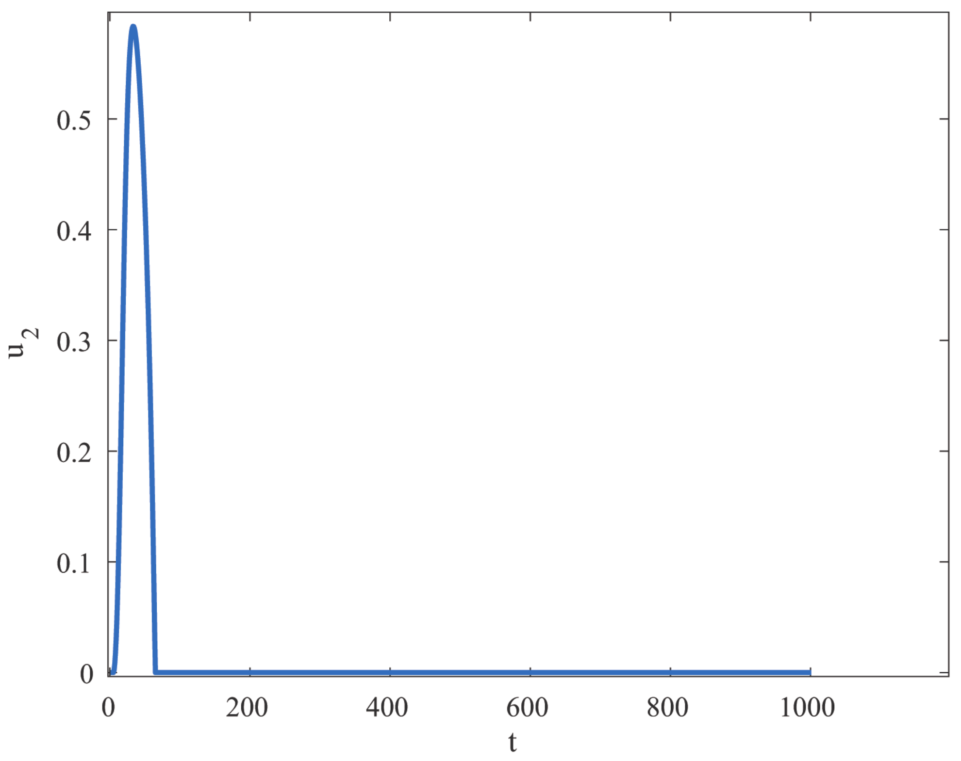
The COVID-19 model, as presented in Equation (6), is subjected to the optimal control strategy. To reduce coronavirus infection and further propagation in the population, we explore four potential controls. These controls can be categorized as follows: the vaccine is specified as the control variable u 1 , and the treatment of the infected human population is defined as the control variable u 2 .
Consider the model (6) with optimal control variables u 1 and u 2 .
0 FFP D κ , λ S ( t ) = υ ( u 1 + τ ) S ( t ) ϑ S ( t ) I ( t ) 1 + ω I ( t ) θ P ( t ) , 0 FFP D κ , λ I ( t ) = ϑ S ( t ) I ( t ) 1 + ω I ( t ) ( τ + u 2 + ν + ϱ 1 ) I ( t ) , 0 FFP D κ , λ Q ( t ) = ν I ( t ) ( τ + ϖ + ϱ 2 ) Q ( t ) , 0 FFP D κ , λ P ( t ) = u 1 S ( t ) + u 2 I ( t ) + ϖ Q ( t ) τ P ( t ) θ P ( t ) , 0 FFP D κ , λ D I Q = ϱ 1 I ( t ) + ϱ 2 Q ( t ) .
The primary aim is to reduce the objective function, which is defined as a function of the state variables subject to non-negativity constraints and non-negative initial conditions.
J u 1 , u 2 = 0 T f z 1 I + z 2 Q + 1 2 B 4 u 1 2 + B 5 u 2 2 d t ,
subject to the control system (34). The parameters governing weight and balance are denoted by the constants B j , where j ranges from 1 to 5, and the terminal time is denoted by T f . Due to the nonlinearity of the control cost associated with intervention, quadratic control functions are employed, indicating that the relationship between the cost of intervention for infected individuals and the impact of intervention is not linear. The aforementioned controls are Lebesgue-integrable functions that are bounded. Our objective is to obtain optimal controls u i * for i equal to 1 or 2.
J u i * = min U J u i ,
where U is denoted to be the control set given by
U = ( u i ) : 0 , T f [ 0 , 1 ] , ( u i ) , is Lebesgue measurable .

Characterization of an Optimal Control

The theory of Pontryagin’s maximum principle [21] provides the necessary requirements that an optimal control must meet. The systems (34) and (35) are transformed into a problem of minimizing a Hamiltonian H pointwise with regard to the controls u i , i = 1 , 2 using this principle. To begin, we must write the Hamiltonian H, which is given by
H = z 1 I + z 2 Q 1 2 + ρ 1 u 1 2 + ρ 2 u 2 2 + Φ 1 υ ( u 1 + τ ) S ( t ) ϑ S ( t ) I ( t ) 1 + ω I ( t ) θ P ( t ) + Φ 2 ϑ S ( t ) I ( t ) 1 + ω I ( t ) ( τ + u 2 + ν + ϱ 1 ) I ( t ) + Φ 3 ν I ( t ) ( τ + ϖ + ϱ 2 ) Q ( t ) + Φ 4 u 1 S ( t ) + u 2 I ( t ) + ϖ Q ( t ) τ P ( t ) θ P ( t ) + Φ 5 ϱ 1 I ( t ) + ϱ 2 Q ( t ) ,
where Φ i for i = 1 , , 5 denote the adjoint variables associated to the state variables S , I , Q , P , and R. For each state variable, the adjoint system can be obtained by taking partial derivatives of the Hamiltonian (38) with respect to the state variables.
Theorem 5.
If the control system (38) is minimized over U by the given optimal controls u i and solutions S , I , Q , P , D , then there exist adjoint variables λ i that satisfy the equation Φ i d t = H i , with the transversal conditions given by
Φ i T f = 0 , i = S , I , Q , P , D .
Now, consider the characteristic equations of the control variables, such that
u 1 : = ρ 1 u 1 + Φ 4 S * Φ 1 S * = 0 , u 2 : = ρ 2 u 2 I * Φ 2 + I * Φ 4 = 0 .
and the optimality condition is given by H u i = 0 , i = 1 , , 4 . Furthermore, we have the controls u i *
u 1 * = min 1 , max 0 , S * Φ 1 Φ 4 ρ 1 , u 2 * = min 1 , max 0 , I * Φ 2 Φ 4 ρ 2 .
Proof. 
The findings of Fleming and Rishel [22] and Sinan et al. [23] provide assurance regarding the presence of an optimal control problem and the corresponding adjoint system, which are derived through the partial derivatives of the Hamiltonian H in Equation (35) and the assessment of the optimal control variables u 1 and u 2 , respectively.
0 FFP D κ , λ Φ 1 ( t ) = Φ 4 u 1 Φ 1 τ + u 1 + I * ϑ I * ω + 1 + I * Φ 2 ϑ I * ω + 1 , 0 FFP D κ , λ Φ 2 ( t ) = z 1 + Φ 5 ϱ 1 + Φ 3 ν + Φ 4 u 2 Φ 2 ϱ 1 + ν + τ + u 2 S * ϑ I * ω + 1 + I * S * ω ϑ I * ω + 1 2 Φ 1 S * ϑ I * ω + 1 2 , 0 FFP D κ , λ Φ 3 ( t ) = z 2 + Φ 5 ϱ 2 + Φ 4 ϖ Φ 3 ϱ 2 + τ + ϖ , 0 FFP D κ , λ Φ 4 ( t ) = Φ 1 θ Φ 4 τ + θ , 0 FFP D κ , λ Φ 5 ( t ) = 0 .
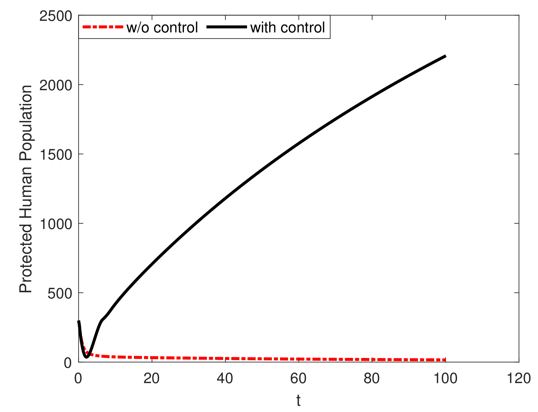
This completes the proof. For the graphical representation of the optimal control we provide Figure 2 and Figure 3 in which the vaccination and treatment rate show best results in protected population P ( t ) . □

7. Numerical Scheme for the Fractal-Fractional Model

Consider the fractal-fractional model (6) and apply the scheme such that
0 FFP D κ , λ S ( t ) = υ τ S ( t ) ϑ S ( t ) I ( t ) 1 + ω I ( t ) , 0 FFP D κ , λ I ( t ) = ϑ S ( t ) I ( t ) 1 + ω I ( t ) ( τ + χ + ν + ϱ 1 ) I ( t ) , 0 FFP D κ , λ Q ( t ) = ν I ( t ) ( τ + ϖ + ϱ 2 ) Q ( t ) , 0 FFP D κ , λ P ( t ) = χ I ( t ) + ϖ Q ( t ) τ P ( t ) , 0 FFP D κ , λ D I Q = ϱ 1 I ( t ) + ϱ 2 Q ( t ) .
Now, the system of Equation (43) implies that
S ( t ) = S ( 0 ) + κ Γ ( λ ) 0 t r κ 1 ( t x ) λ 1 v 1 S , x d x , I ( t ) = I ( 0 ) + κ Γ ( λ ) 0 t r κ 1 ( t x ) λ 1 v 2 I , x d x , Q ( t ) = Q ( 0 ) + κ Γ ( λ ) 0 t r κ 1 ( t x ) λ 1 v 3 Q , x d x , P ( t ) = P ( 0 ) + κ Γ ( λ ) 0 t r κ 1 ( t x ) λ 1 v 4 P , x d x , D I Q ( t ) = D I Q ( 0 ) + κ Γ ( λ ) 0 t r κ 1 ( t x ) λ 1 v 5 D I Q , x d x .
The resultant scheme for the system (44) is given as
S ( m + 1 ) = S ( 0 ) + κ λ Γ ( λ + 2 ) p = 0 m t ( p ) κ 1 v S ( p ) , t p × ( m + 1 p ) κ ( m p + 2 + κ ) ( m p ) κ ( m p + 2 + 2 κ ) t ( p 1 ) κ 1 v S ( p 1 ) , t ( p 1 ) ( m + 1 p ) κ + 1 ( m p ) κ ( m p + 1 + κ ) ,
I ( m + 1 ) = I ( 0 ) + κ λ Γ ( λ + 2 ) p = 0 m t ( p ) κ 1 v I ( p ) , t p × ( m + 1 p ) κ ( m p + 2 + κ ) ( m p ) κ ( m p + 2 + 2 κ ) t ( p 1 ) κ 1 v I ( p 1 ) , t ( p 1 ) ( m + 1 p ) κ + 1 ( m p ) κ ( m p + 1 + κ ) ,
Q ( m + 1 ) = Q ( 0 ) + κ λ Γ ( λ + 2 ) p = 0 m t ( p ) κ 1 v Q ( p ) , t p × ( m + 1 p ) κ ( m p + 2 + κ ) ( m p ) κ ( m p + 2 + 2 κ ) t ( p 1 ) κ 1 v Q ( p 1 ) , t ( p 1 ) ( m + 1 p ) κ + 1 ( m p ) κ ( m p + 1 + κ ) ,
P ( m + 1 ) = P ( 0 ) + κ λ Γ ( λ + 2 ) p = 0 m t ( p ) κ 1 v P ( p ) , t p × ( m + 1 p ) κ ( m p + 2 + κ ) ( m p ) κ ( m p + 2 + 2 κ ) t ( p 1 ) κ 1 v P ( p 1 ) , t ( p 1 ) ( m + 1 p ) κ + 1 ( m p ) κ ( m p + 1 + κ ) ,
D I Q ( m + 1 ) = D I Q ( 0 ) + κ λ Γ ( λ + 2 ) p = 0 m t ( p ) κ 1 v D I Q ( p ) , t p × ( m + 1 p ) κ ( m p + 2 + κ ) ( m p ) κ ( m p + 2 + 2 κ ) t ( p 1 ) κ 1 v D I Q ( p 1 ) , t ( p 1 ) ( m + 1 p ) κ + 1 ( m p ) κ ( m p + 1 + κ ) .

8. Results and Discussion

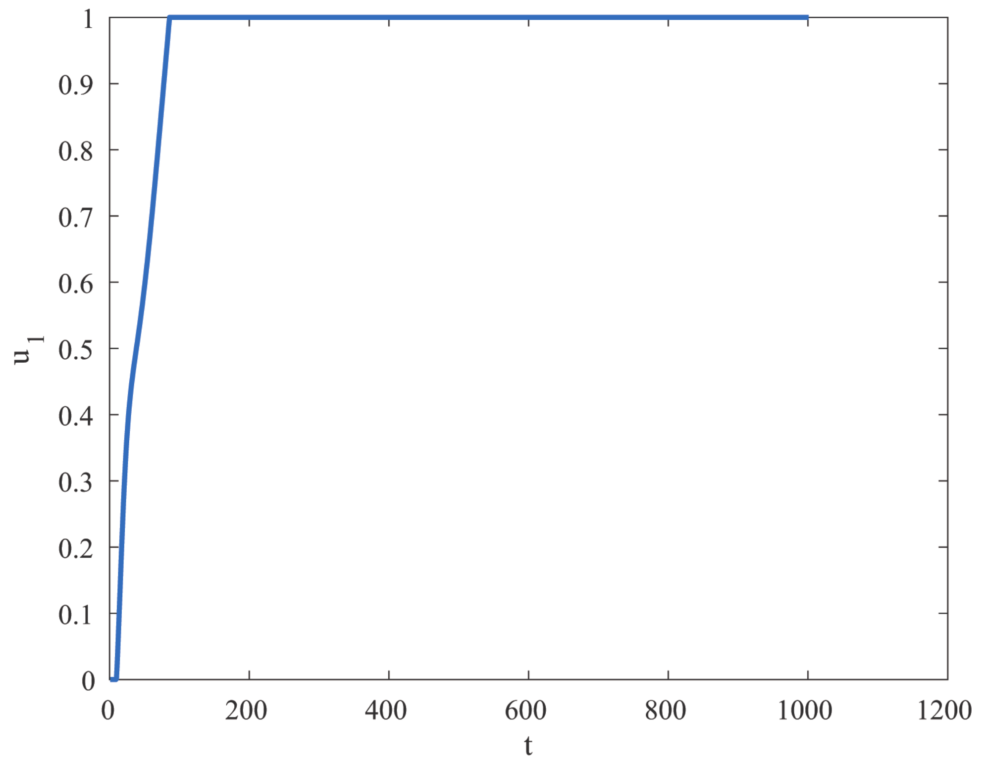
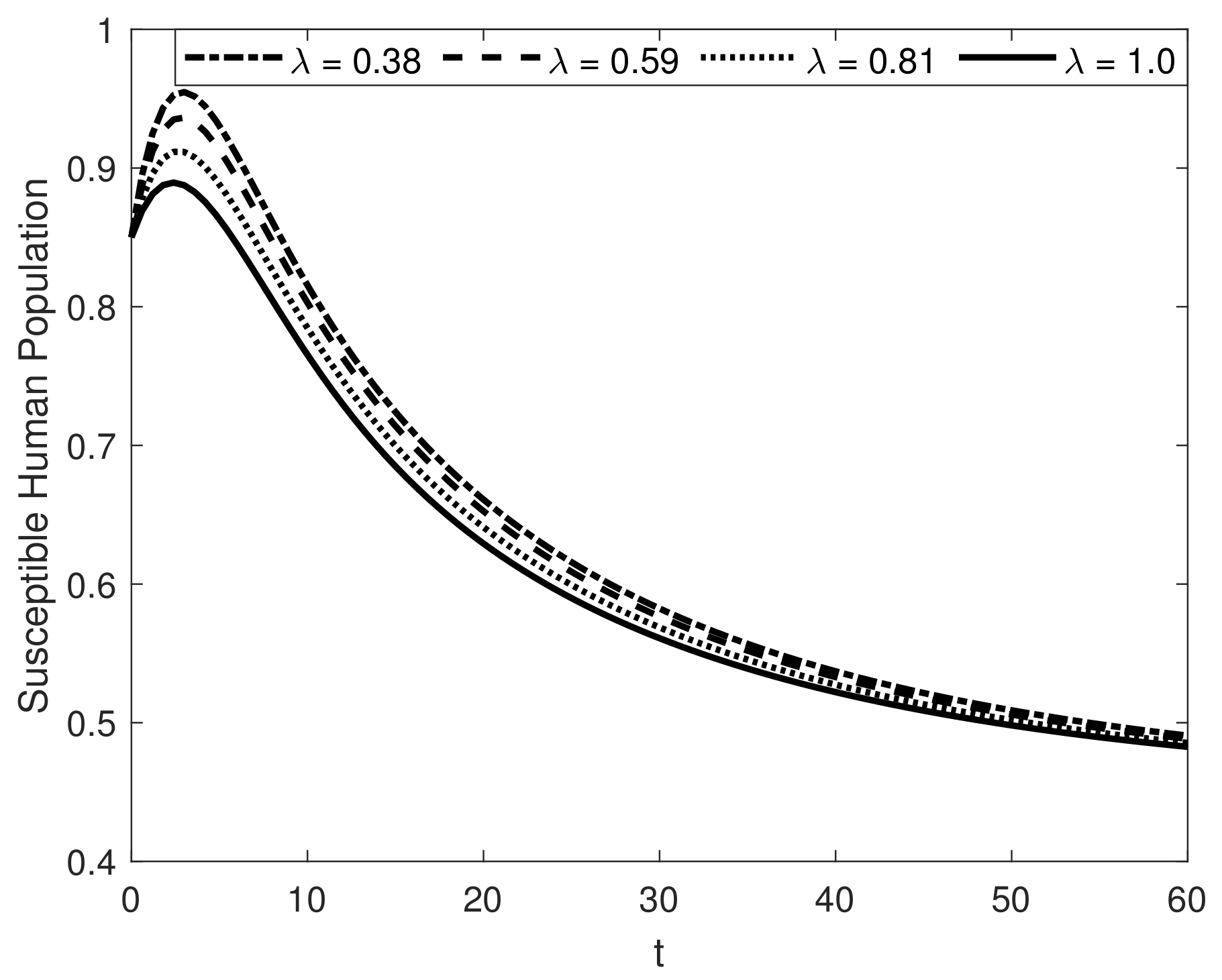
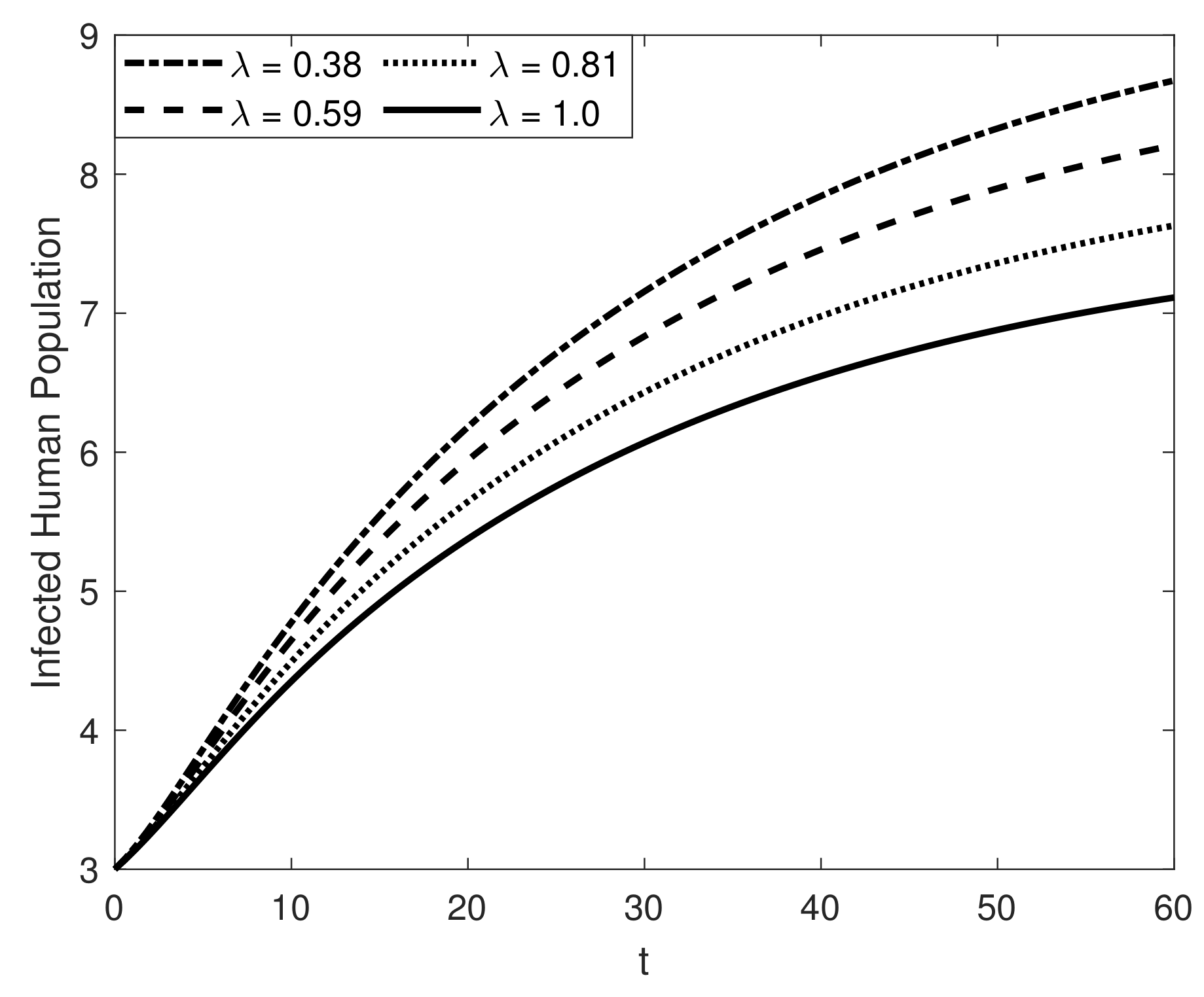
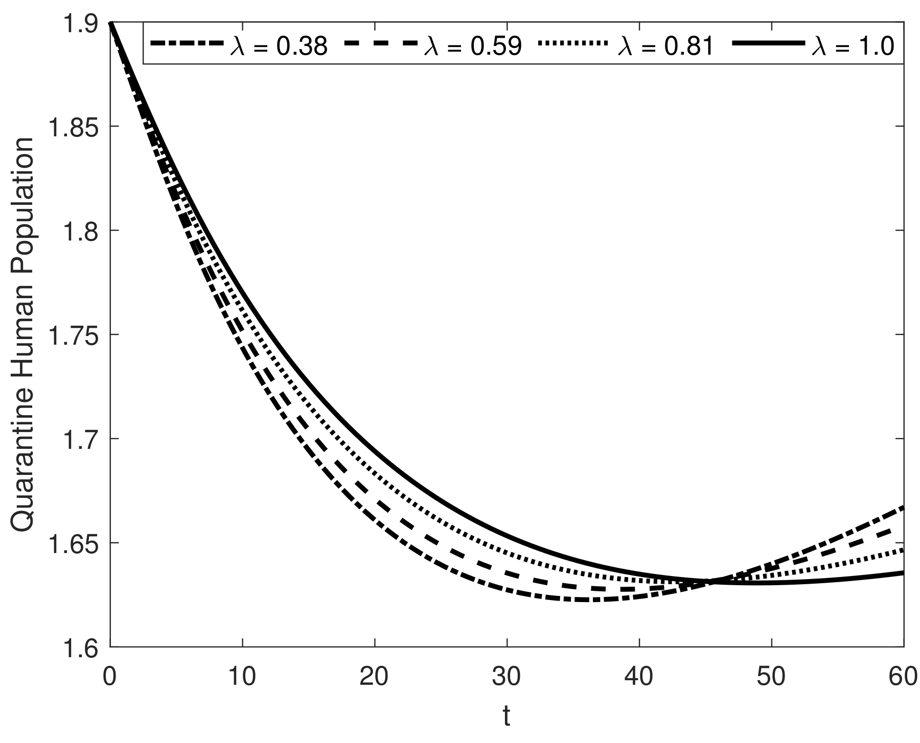
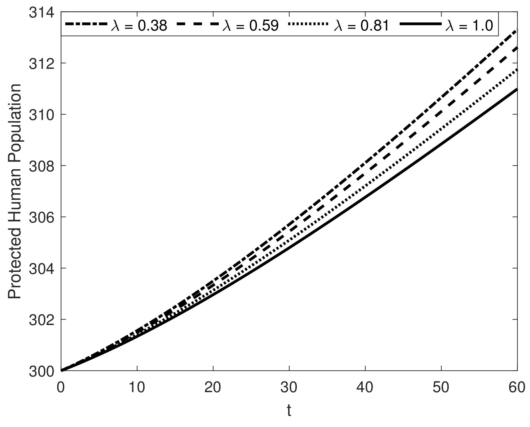
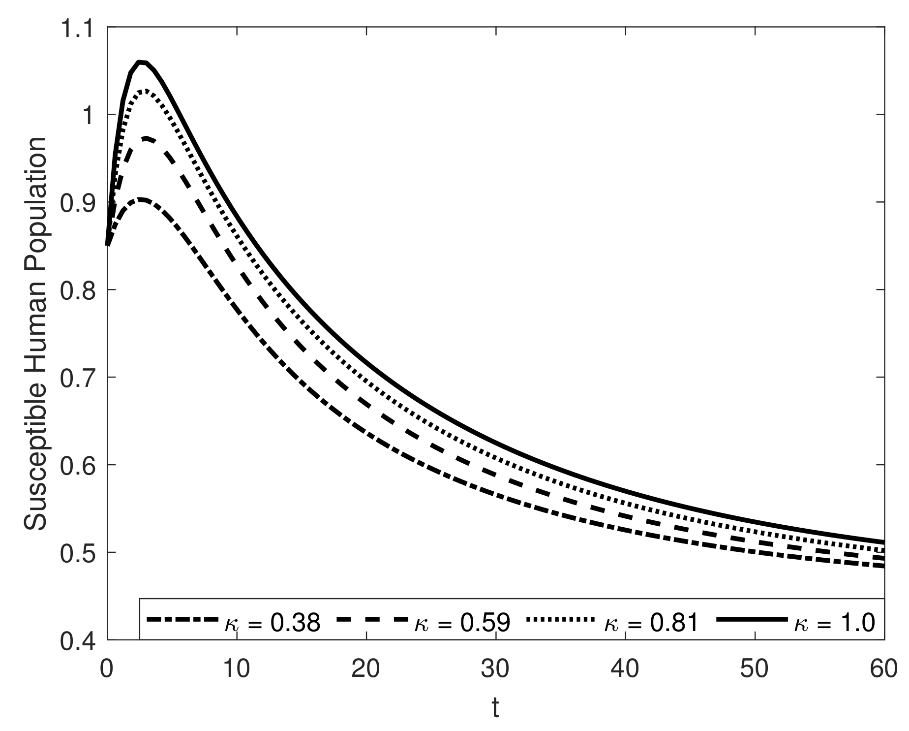
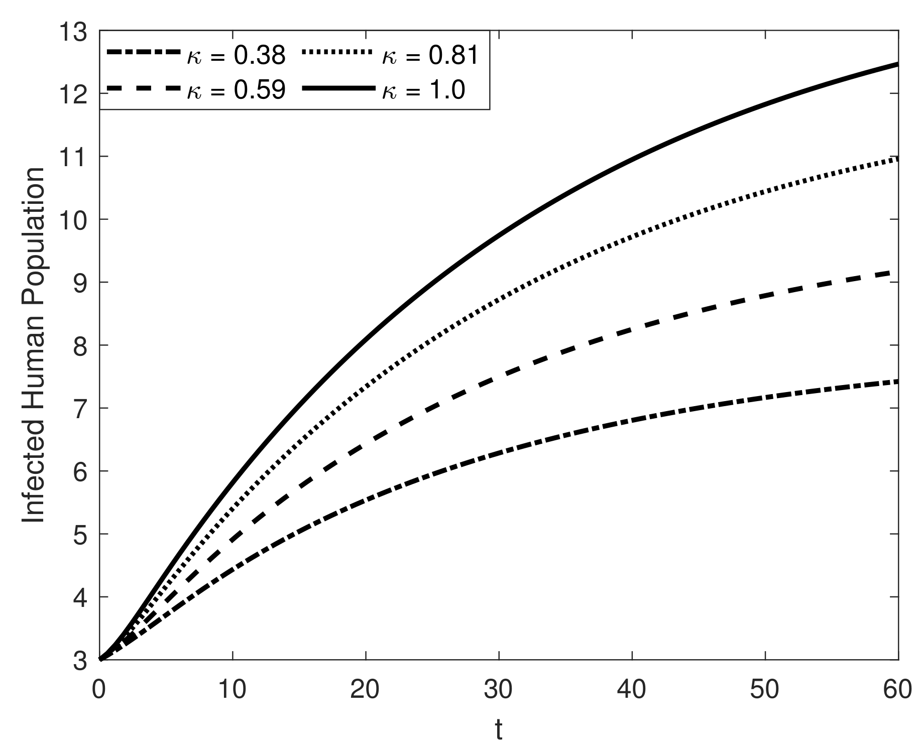
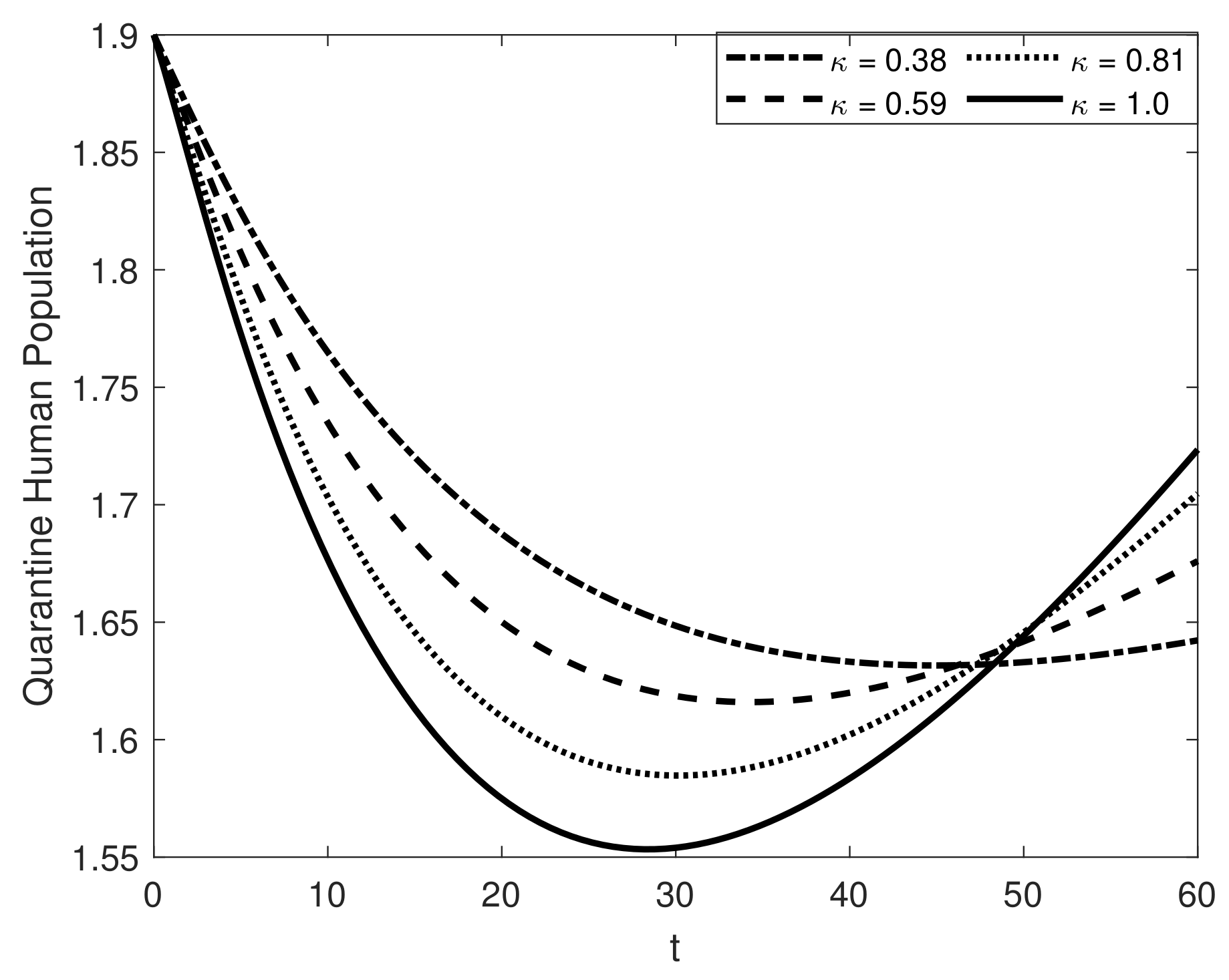
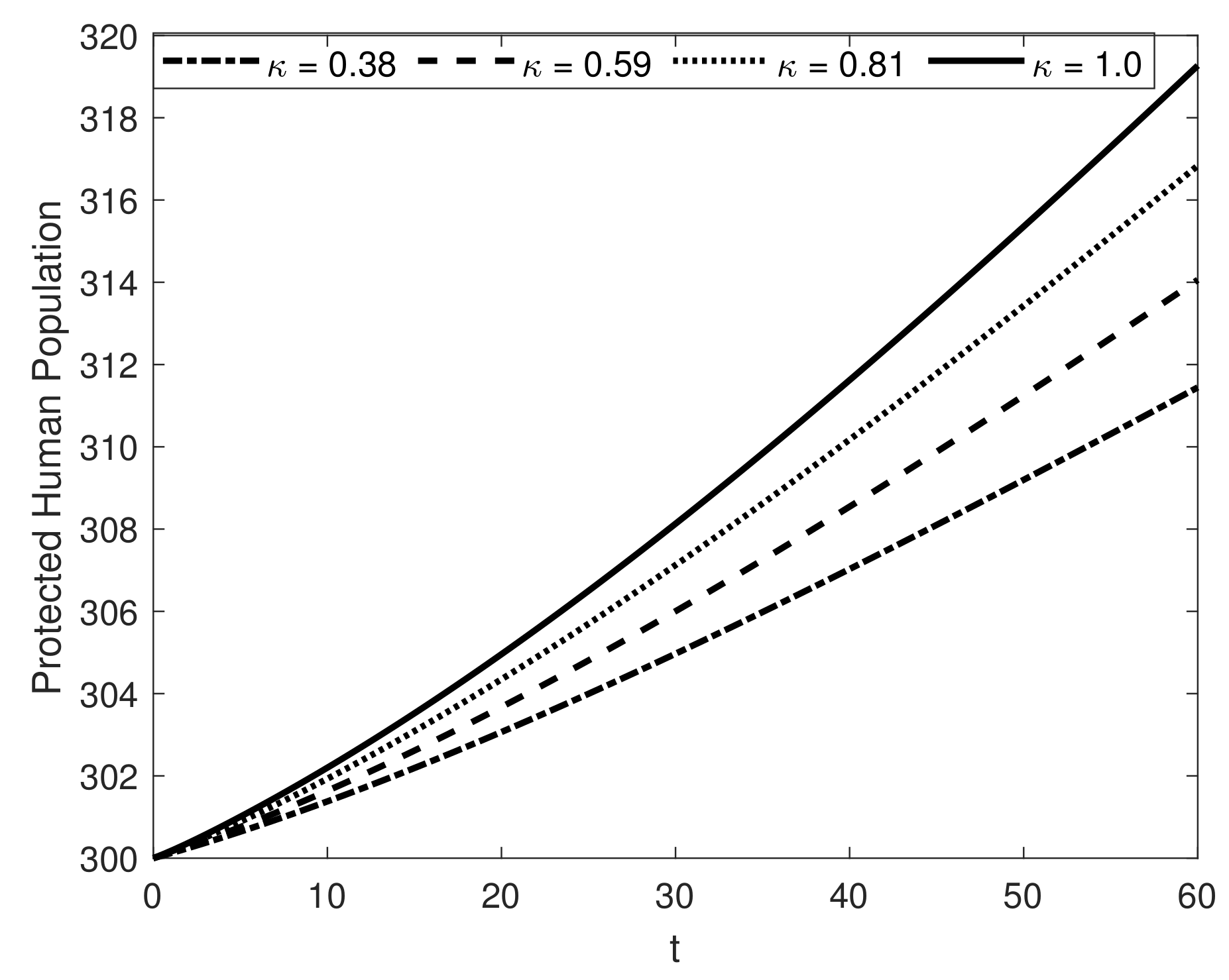
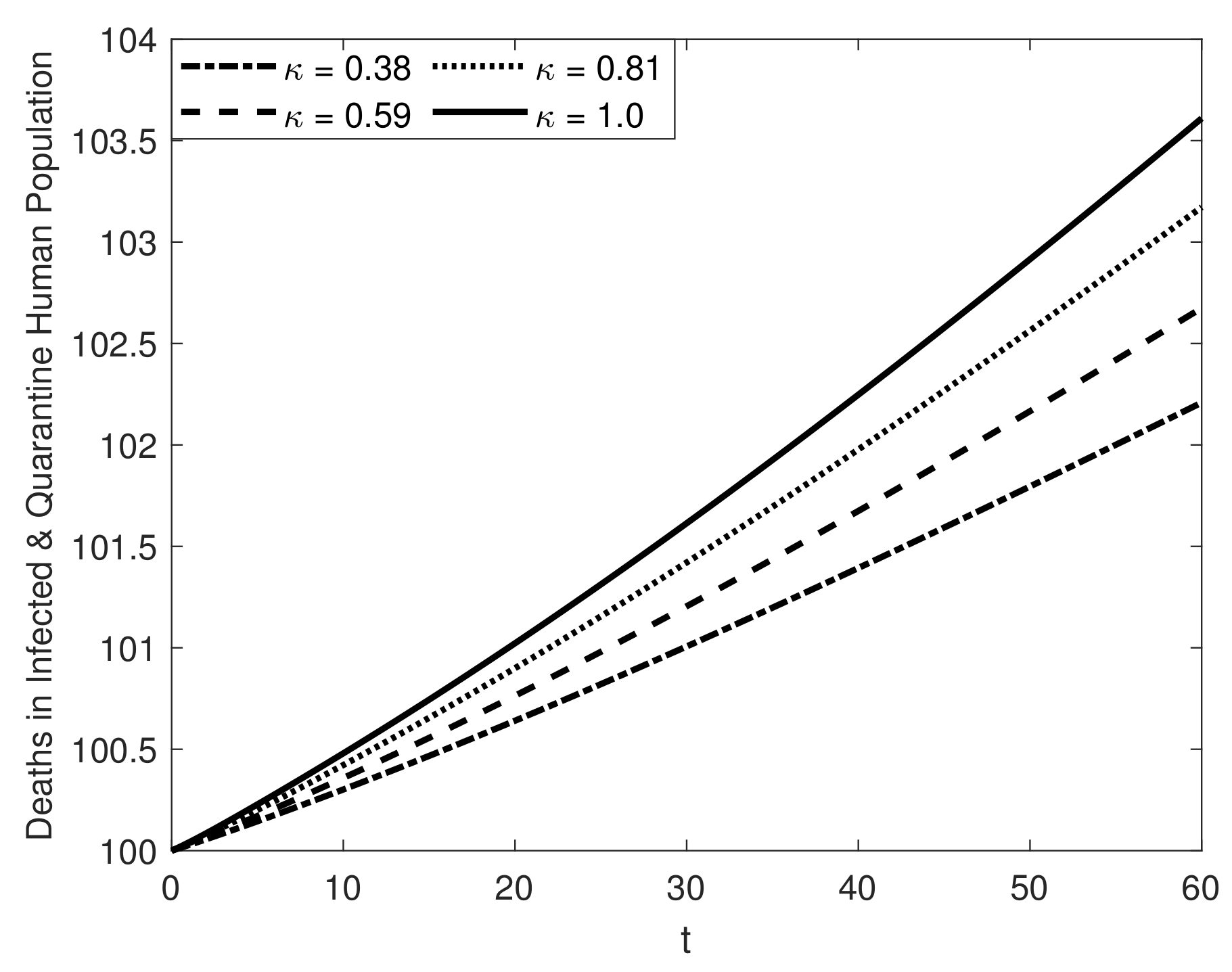
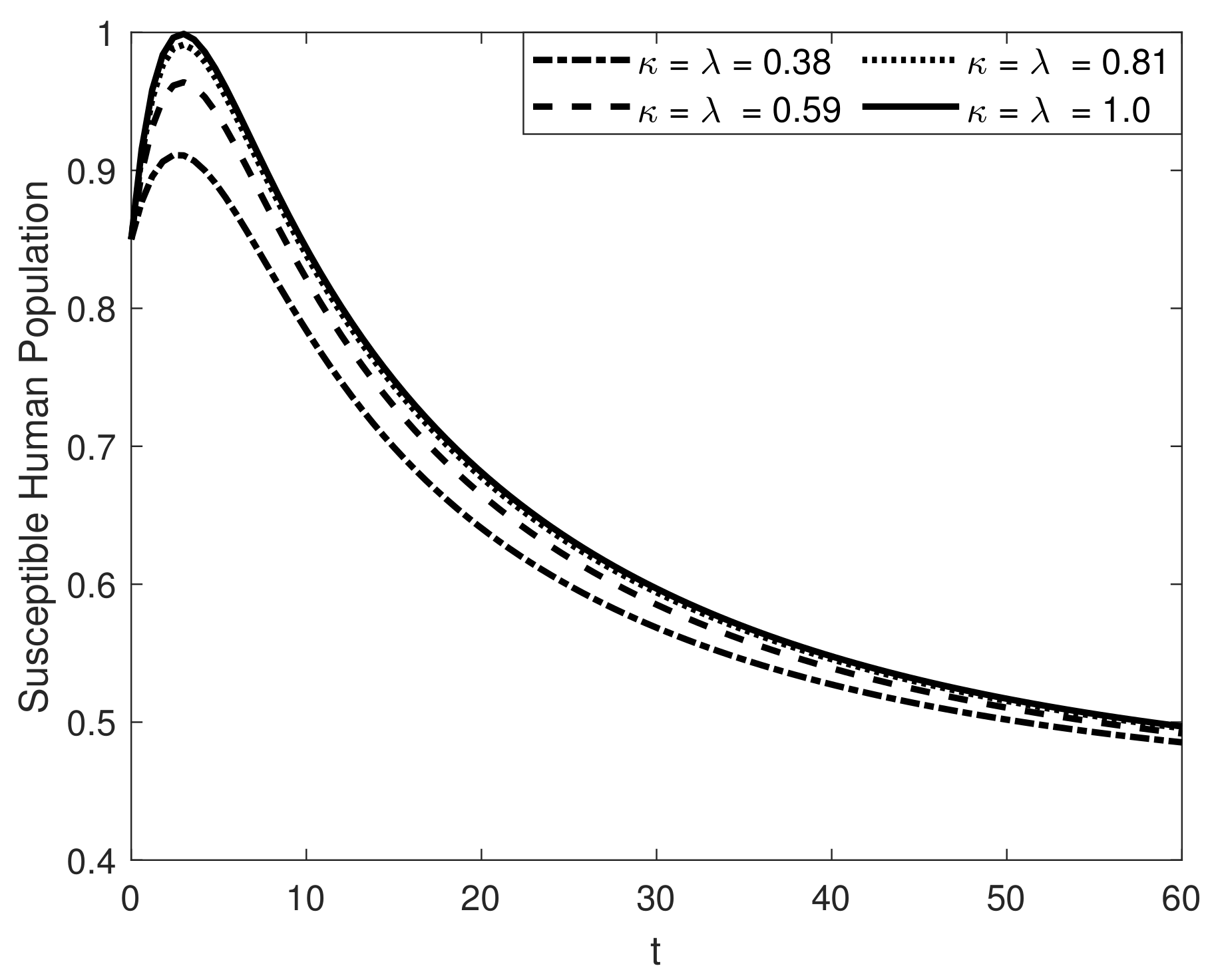
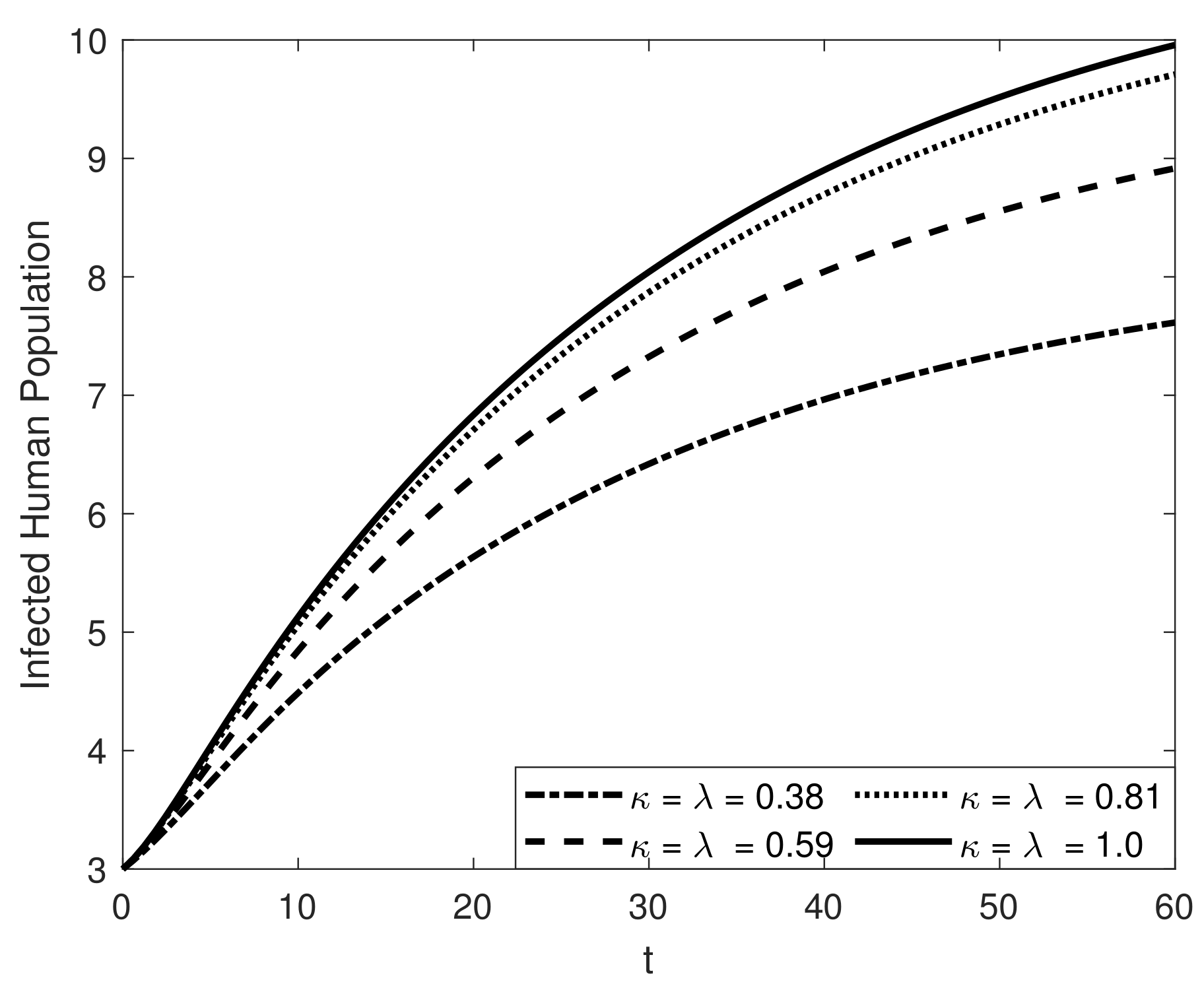
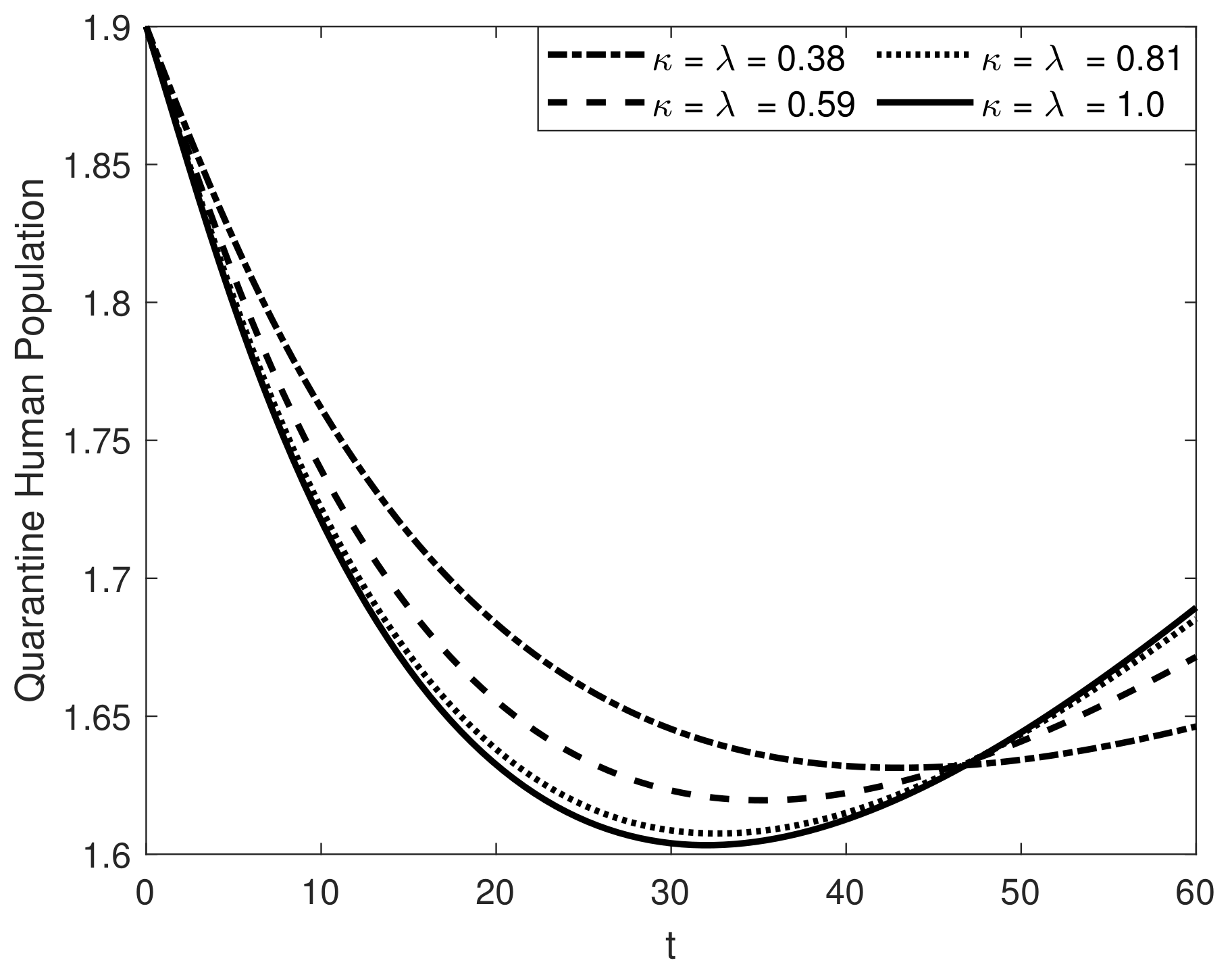
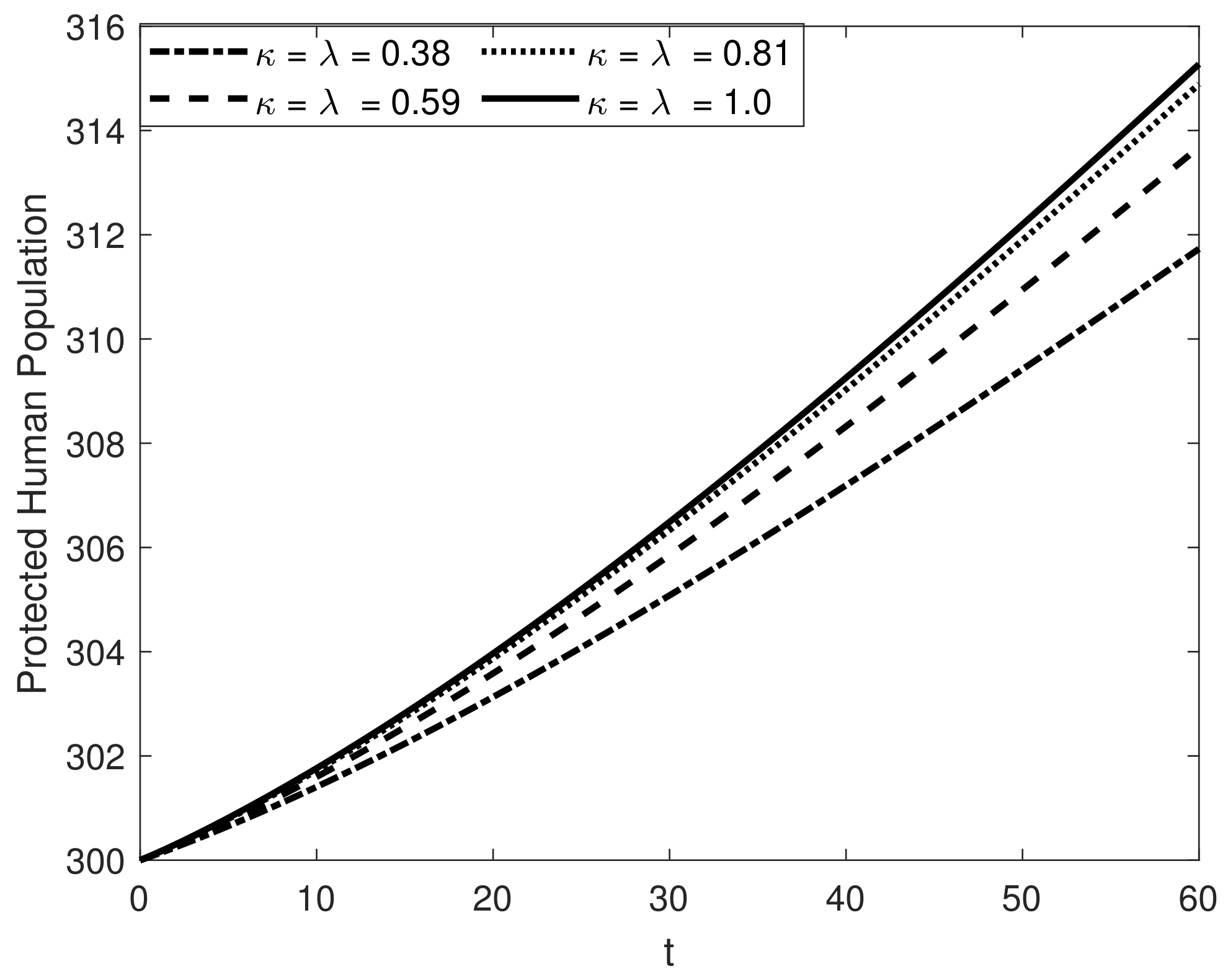
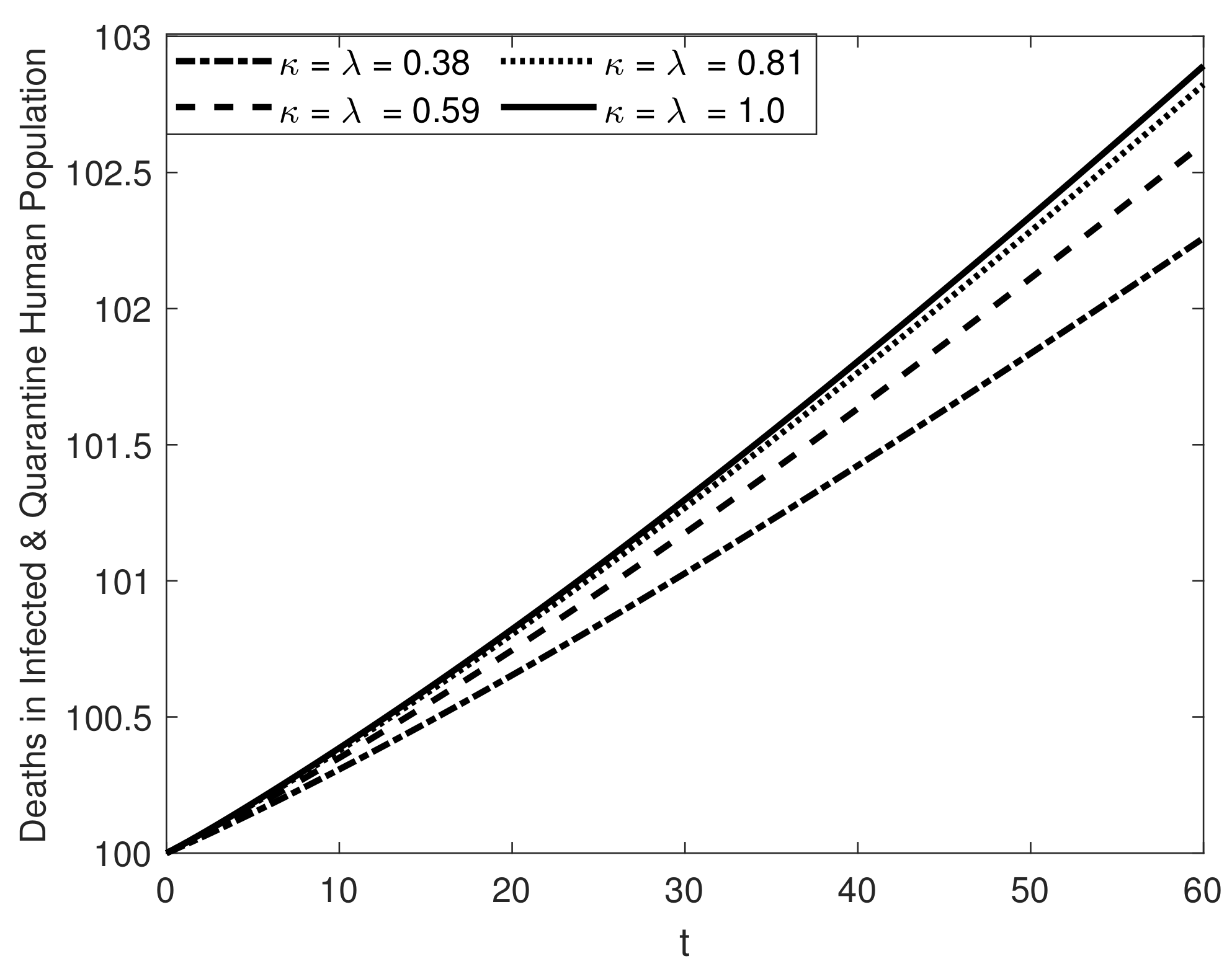
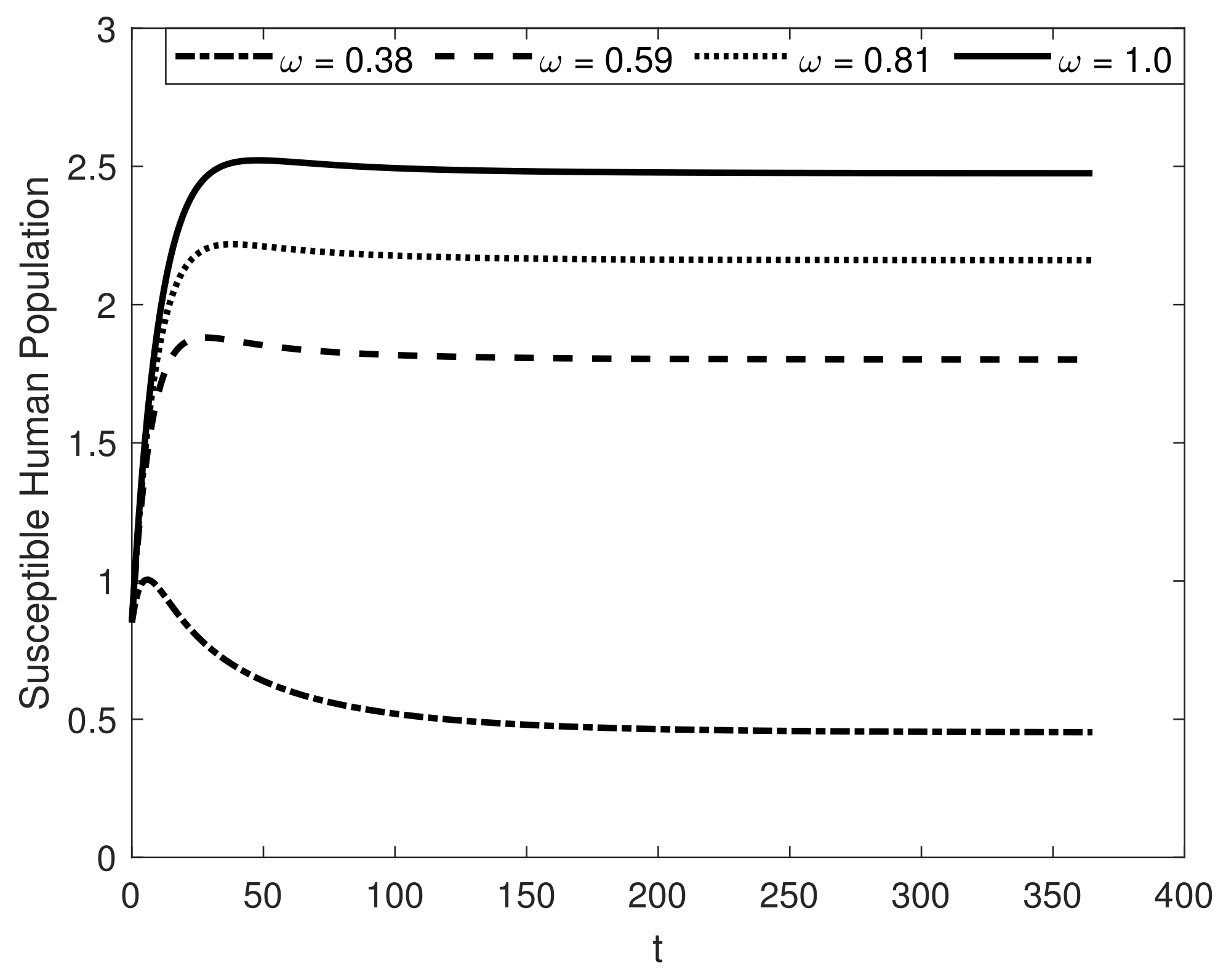
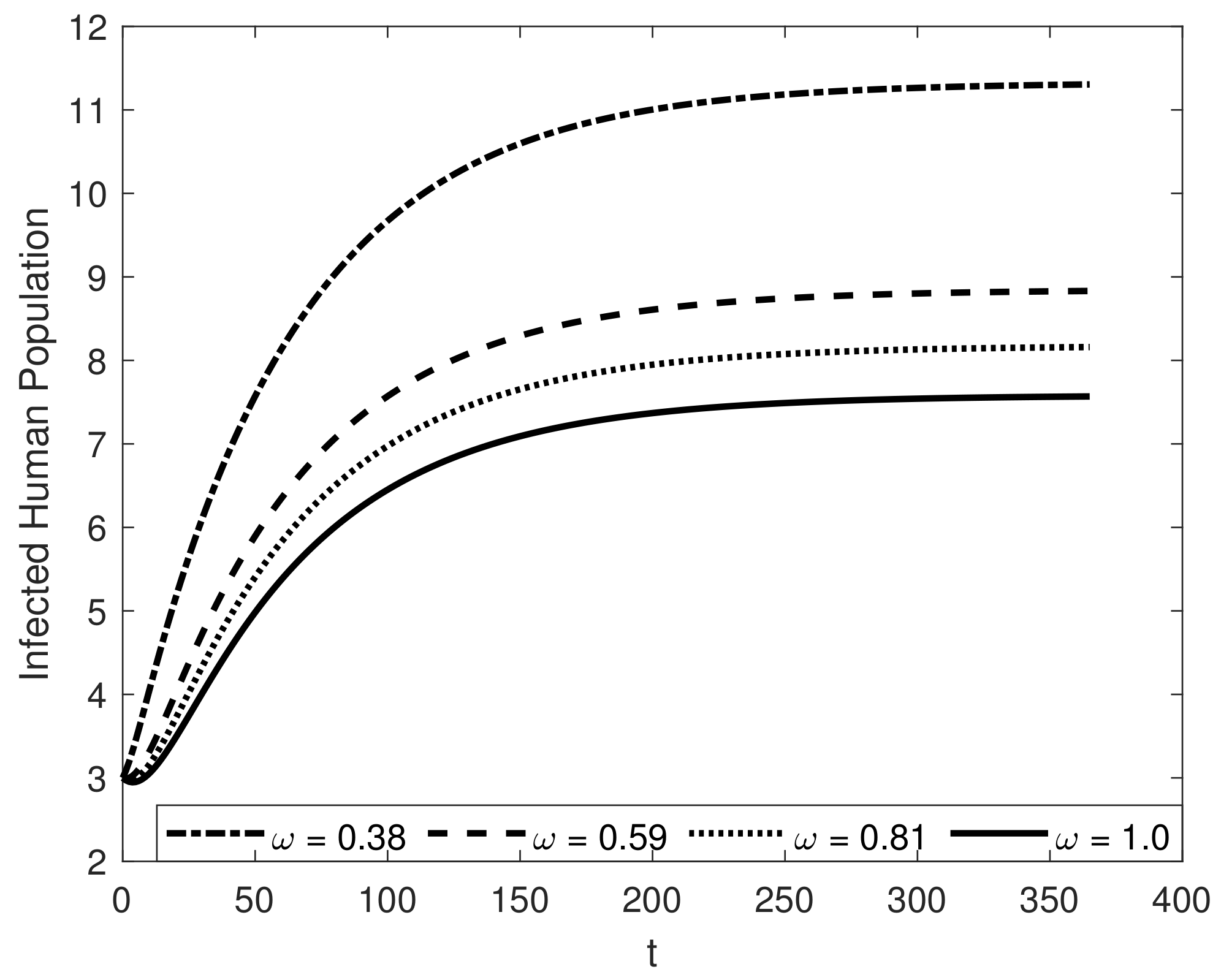
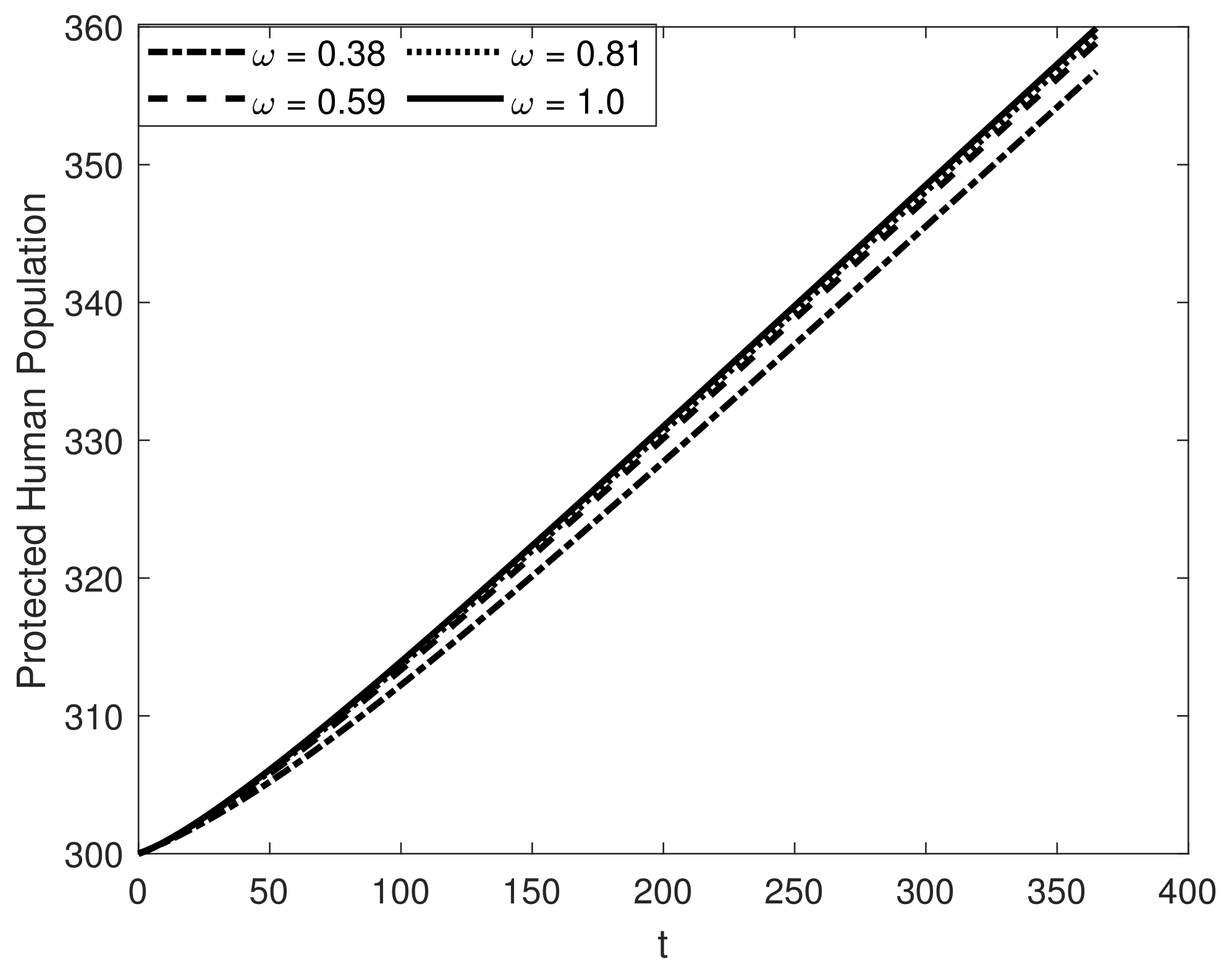
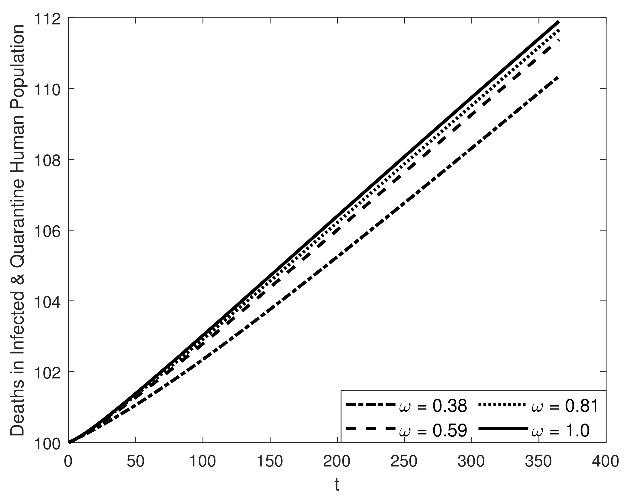
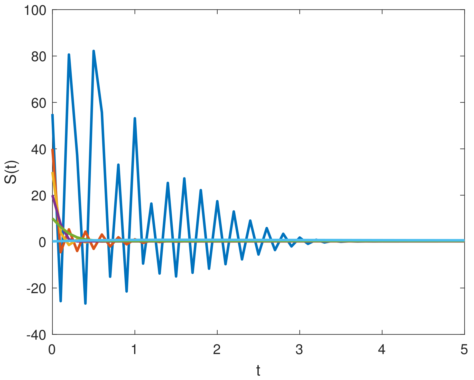
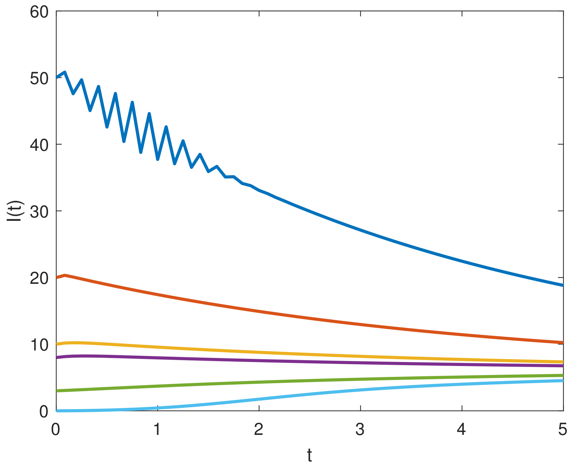
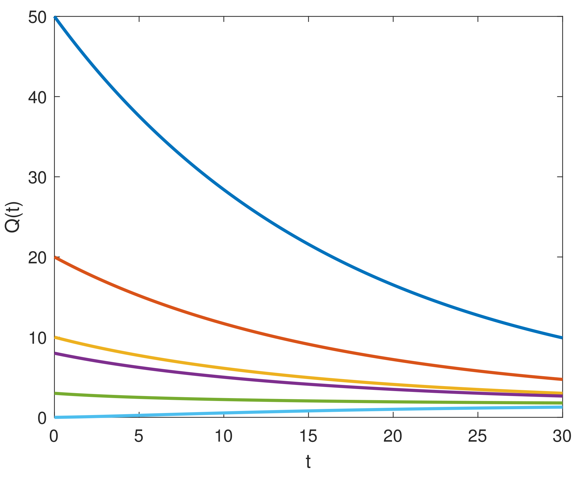
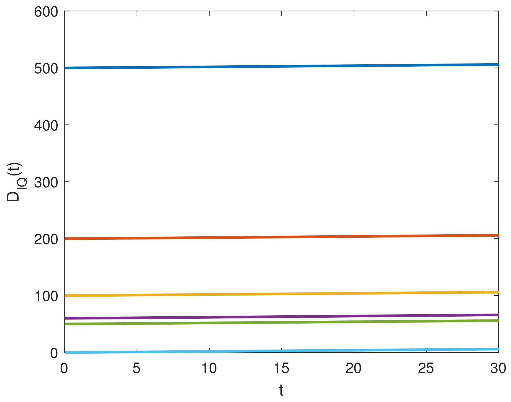
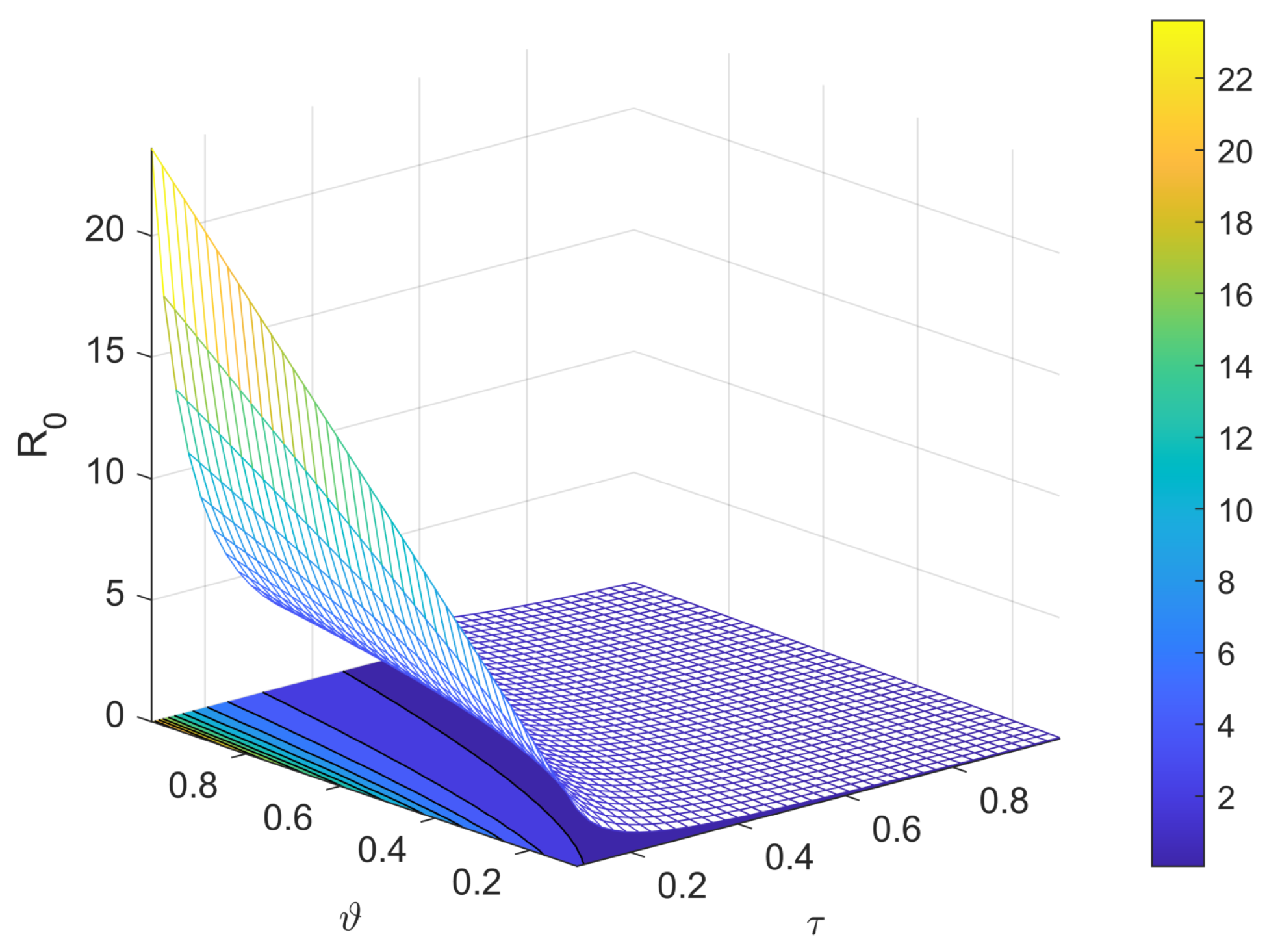
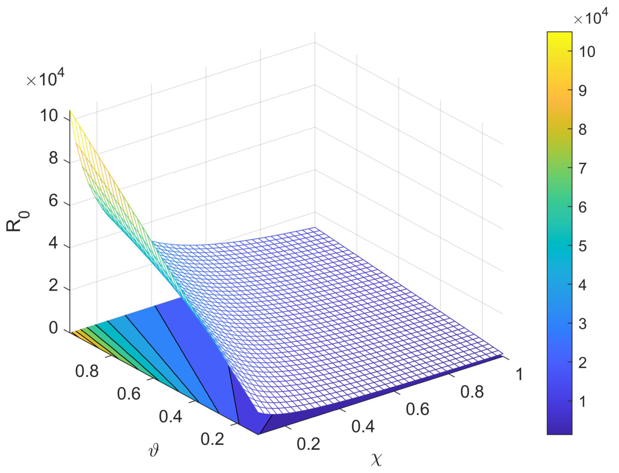
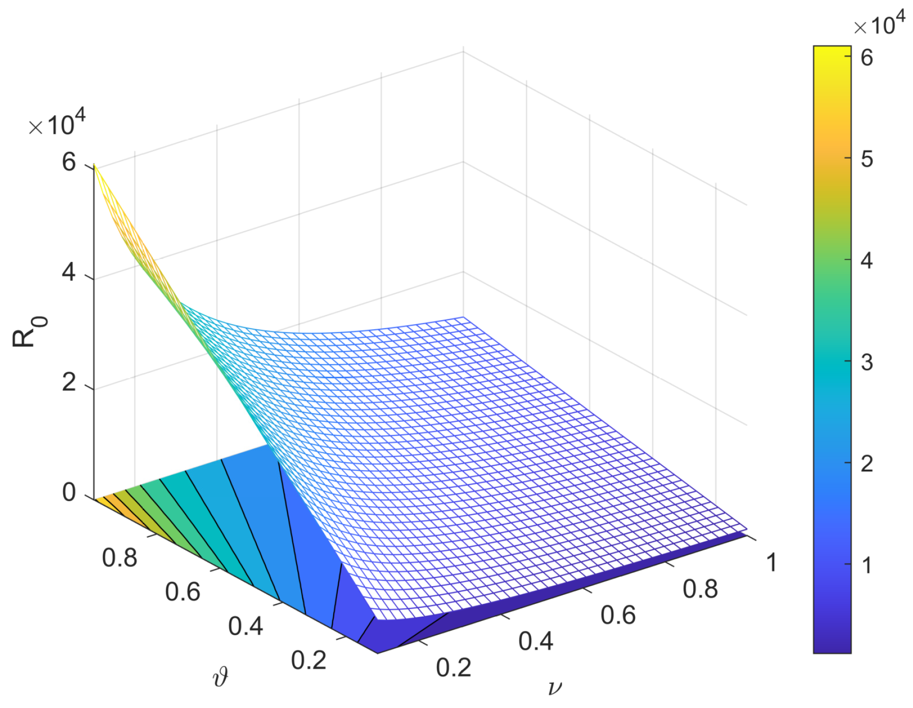
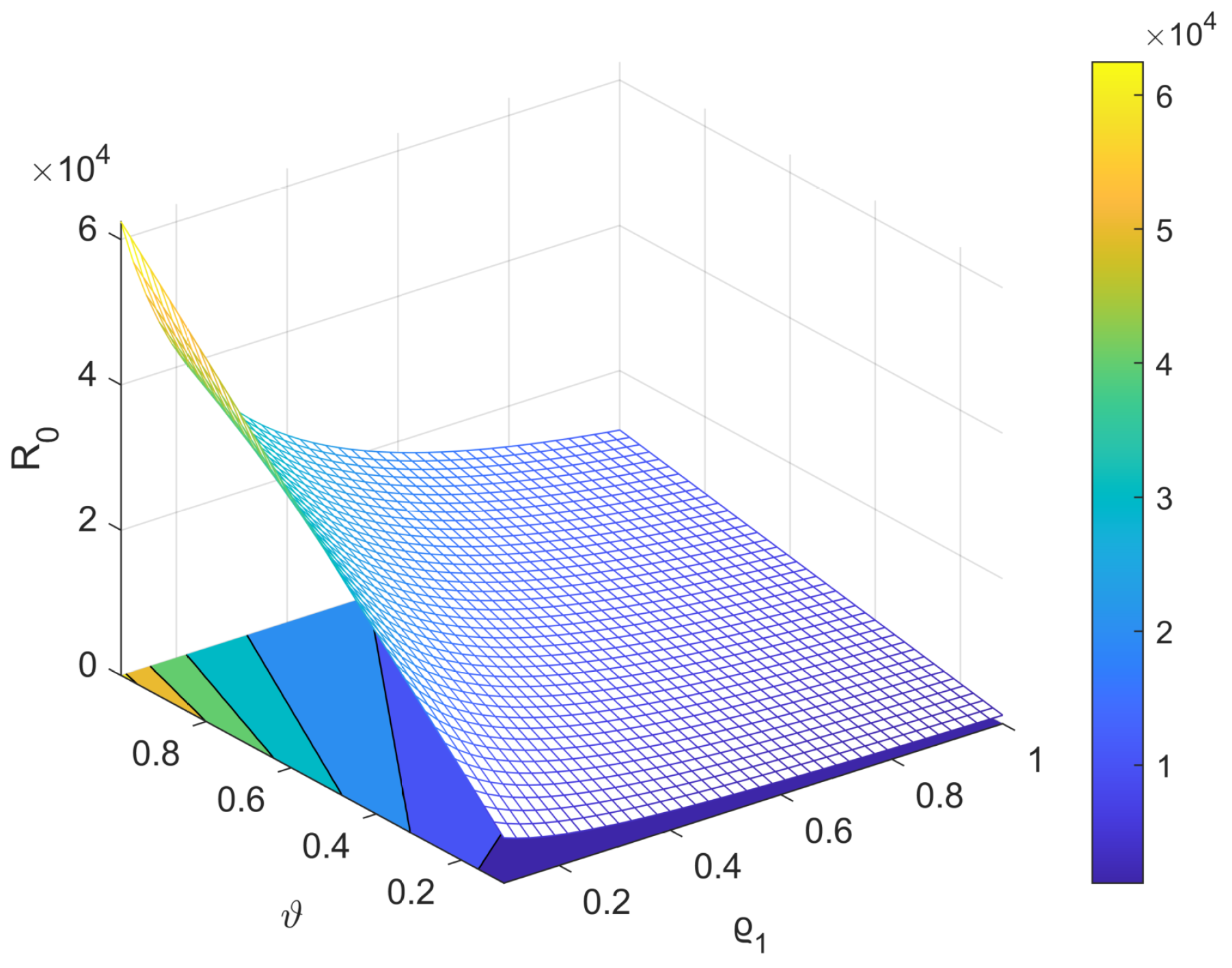
We have simulated our model for various values of fractal dimensions and different fractional orders, and the results are presented in Figure 4, Figure 5, Figure 6, Figure 7, Figure 8, Figure 9, Figure 10, Figure 11, Figure 12, Figure 13, Figure 14, Figure 15, Figure 16, Figure 17, Figure 18, Figure 19, Figure 20, Figure 21, Figure 22, Figure 23, Figure 24, Figure 25, Figure 26, Figure 27, Figure 28, Figure 29, Figure 30 and Figure 31. To protect the human population from reinfection and treat infected humans in hospitals, we implemented an optimal control strategy using Pontryagin’s maximum principle, as used by [24,25,26]. Two optimal control variables, u 1 and u 2 , were employed to represent vaccination of the susceptible class and treatment of the infected class, respectively. The resulting figure, shown in Figure 2, demonstrates an increase in the protected human population for fractal-fractional orders with κ = 0.5 and λ = 0.5 . The control variables are presented in Figure 3 and Figure 32. A sensitivity analysis was conducted on each parameter’s basic reproduction number, and the findings were displayed in a bar chart in Figure 1. Additionally, Figure 4, Figure 5, Figure 6, Figure 7 and Figure 8 present three-dimensional plots of each parameter. The results of the sensitivity analysis indicate that the parameters τ , ϑ , χ , and υ are more sensitive than the other parameters. The behaviour of surfaces in Figure 33, Figure 34, Figure 35, Figure 36 and Figure 37 show the effect in R 0 due to the variation in parameters υ and ϑ , τ and ϑ , χ and ϑ , ν and ϑ while ϱ 1 and ϑ . By examining the sensitivity of certain parameters, a meaningful connection can be established among the uncertain parameters in the model. From Figure 19, Figure 20, Figure 21 and Figure 22, it reflects that the COVID-19 pandemic has had a significant impact on the mental health and well-being of people worldwide. The uncertainty, fear, and stress caused by the pandemic have led to a range of psychological effects, including: Anxiety and Depression: The pandemic has caused a lot of anxiety and depression among people due to the fear of getting infected, losing loved ones, and the uncertainty of the future. Social Isolation: The pandemic has led to social distancing measures, which have resulted in social isolation and loneliness, leading to depression and anxiety. Post-Traumatic Stress Disorder (PTSD): People who have been infected with COVID-19 or have lost loved ones to the virus may develop PTSD, which can cause flashbacks, nightmares, and anxiety. Substance Abuse: The pandemic has led to an increase in substance abuse, including alcohol and drug abuse, as people try to cope with the stress and anxiety caused by the pandemic. Burnout: Healthcare workers and essential workers have been working tirelessly during the pandemic, leading to burnout and exhaustion. Overall, the COVID-19 pandemic has had a significant impact on the mental health and well-being of people worldwide. So, the factors described above can cause deaths.

9. Conclusions

In this manuscript, we have established a comprehensive analysis for a fractal-fractional-type model addressing the COVID-19 disease. We have computed the fundamental threshold number, which allows us to predict the transmission of the disease in the community. Additionally, we have carried out a sensitivity analysis of some parameters in the considered model and developed a bifurcation analysis for the proposed model. Bifurcation analysis is a powerful procedure to investigate the steady-state nonlinear dynamics of systems, and we have used the methodology adopted by Castillo-Chavez and Song. We have also established an optimal control strategy using Pontryagin’s maximum principle in the proposed model. Finally, we have simulated the proposed model by considering various values of fractal and fractional order corresponding to some real values. The sensitivity and bifurcation analysis of the dynamical system enables us to investigate the abrupt qualitative changes in the considered system, and the fractal-fractional order derivative allows for a more precise explanation of the dynamics. In the future, the analysis established in this paper can be extended to a more complex biological model. The coronavirus pandemic has had a significant impact on the mental health and well-being of people worldwide. The fear and uncertainty surrounding the virus, coupled with the social isolation and economic stress caused by lockdowns and restrictions, have led to increased levels of anxiety, depression, and other mental health issues. People have also experienced grief and loss due to the death of loved ones, as well as the loss of jobs, businesses, and social connections. The pandemic has also highlighted existing inequalities and disparities in access to healthcare and resources, which can further exacerbate mental health issues. However, it is important to note that people have also shown resilience and adaptability in the face of the pandemic. Many have found ways to cope with the challenges and have even experienced personal growth and positive changes in their lives. Seeking support from mental health professionals, staying connected with loved ones, and practicing self-care can all help mitigate the psychological effects of the pandemic.

Author Contributions

Conceptualization, N.H.A.; Writing—original draft, M.S. All authors have read and agreed to the published version of the manuscript.

Funding

This research was supported by the Deanship of Scientific Research, Imam Mohammad Ibn Saud Islamic University (IMSIU), Saudi Arabia, Grant No. (21-13-18-043).

Data Availability Statement

All the data are within the manuscript.

Acknowledgments

This research was supported by the Deanship of Scientific Research, Imam Mohammad Ibn Saud Islamic University (IMSIO), Saudi Arabia, Grant No. (21-13-18-043).

Conflicts of Interest

The authors have no conflict of interest.

References

  1. Anderson, P.K.; Cunningham, A.A.; Patel, N.G.; Morales, F.J.; Epstein, P.R.; Daszak, P. Emerging infectious diseases of plants: Pathogen pollution, climate change and agrotechnology drivers. Trends Ecol. Evol. 2004, 19, 535–544. [Google Scholar] [CrossRef] [PubMed]
  2. Omame, A.; Isah, M.E.; Abbas, M. An optimal control model for COVID-19, zika, dengue, and chikungunya co-dynamics with reinfection. Optim. Control Appl. Methods 2023, 44, 170–204. [Google Scholar] [CrossRef] [PubMed]
  3. Saha, P.; Biswas, S.K.; Biswas, M.H.A.; Ghosh, U. An SEQAIHR model to study COVID-19 transmission and optimal control strategies in Hong Kong, 2022. Nonlinear Dyn. 2023, 111, 6873–6893. [Google Scholar] [CrossRef] [PubMed]
  4. Anderson, R.M.; May, R.M. Infectious Diseases of Humans: Dynamics and Control; Oxford University Press: Oxford, UK, 1992. [Google Scholar]
  5. Khan, H.; Ahmad, F.; Tunç, O.; Idrees, M. On fractal-fractional COVID-19 mathematical model. Chaos Solitons Fractals 2022, 157, 111937. [Google Scholar] [CrossRef]
  6. Hamou, A.A.; Azroul, E.; Hammouch, Z.; Alaoui, A.L. A fractional multi-order model to predict the COVID-19 outbreak in Morocco. Appl. Comput. Math. 2020, 20, 177–203. [Google Scholar]
  7. Lu, Z.; Yu, Y.; Chen, Y.; Ren, G.; Xu, C.; Wang, S.; Yin, Z. A fractional-order SEIHDR model for COVID-19 with inter-city networked coupling effects. Nonlinear Dyn. 2020, 101, 1717–1730. [Google Scholar] [CrossRef]
  8. Atangana, A.; Qureshi, S. Modeling attractors of chaotic dynamical systems with fractal–fractional operators. Chaos Solitons Fractals 2019, 123, 320–337. [Google Scholar] [CrossRef]
  9. Atangana, A. Fractal-fractional differentiation and integration: Connecting fractal calculus and fractional calculus to predict complex system. Chaos Solitons Fractals 2017, 102, 396–406. [Google Scholar] [CrossRef]
  10. Qureshi, S.; Atangana, A. Mathematical analysis of dengue fever outbreak by novel fractional operators with field data. Phys. Stat. Mech. Its Appl. 2019, 526, 121127. [Google Scholar] [CrossRef]
  11. Li, Z.; Liu, Z.; Khan, M.A. Fractional investigation of bank data with fractal-fractional Caputo derivative. Chaos Solitons Fractals 2020, 131, 109528. [Google Scholar] [CrossRef]
  12. Zhang, L.; ur Rahman, M.; Haidong, Q.; Arfan, M.; Adnan. Fractal-fractional Anthroponotic Cutaneous Leishmania model study in sense of Caputo derivative. Alex. Eng. J. 2021, 61, 4423–4433. [Google Scholar] [CrossRef]
  13. Shen, Z.H.; Chu, Y.M.; Khan, M.A.; Muhammad, S.; Al-Hartomy, O.A.; Higazy, M. Mathematical modeling and optimal control of the COVID-19 dynamics. Results Phys. 2021, 31, 105028. [Google Scholar] [CrossRef]
  14. Liu, S.; Pang, L.; Ruan, S.; Zhang, X. Global dynamics of avian influenza epidemic models with psychological effect. Comput. Math. Methods Med. 2015, 2015, 913726. [Google Scholar] [CrossRef]
  15. Gu, Y.; Khan, M.A.; Hamed, Y.; Felemban, B.F. A Comprehensive Mathematical Model for SARS-CoV-2 in Caputo Derivative. Fractal Fract. 2021, 5, 271. [Google Scholar] [CrossRef]
  16. Lu, H.; Ding, Y.; Gong, S.; Wang, S. Mathematical modeling and dynamic analysis of SIQR model with delay for pandemic COVID-19. Math. Biosci. Eng. 2021, 18, 3197–3214. [Google Scholar] [CrossRef]
  17. Bozdağ, F. The psychological effects of staying home due to the COVID-19 pandemic. J. Gen. Psychol. 2021, 148, 226–248. [Google Scholar] [CrossRef]
  18. Castillo-Chavez, C.; Song, B. Dynamical models of tuberculosis and their applications. Math. Biosci. Eng. 2004, 1, 361. [Google Scholar] [CrossRef]
  19. Buonomo, B.; Lacitignola, D. On the backward bifurcation of a vaccination model with nonlinear incidence. Nonlinear Anal. Model. Control 2011, 16, 30–46. [Google Scholar] [CrossRef]
  20. Chitnis, N.; Hyman, J.M.; Cushing, J.M. Determining important parameters in the spread of malaria through the sensitivity analysis of a mathematical model. Bull. Math. Biol. 2008, 70, 1272–1296. [Google Scholar] [CrossRef]
  21. Pontryagin, L.S. Mathematical Theory of Optimal Processes; CRC Press: Boca Raton, FL, USA, 1987. [Google Scholar]
  22. Fleming, W.H.; Rishel, R.W. Deterministic and Stochastic Optimal Control; Springer Science & Business Media: Berlin/Heidelberg, Germany, 2012; Volume 1. [Google Scholar]
  23. Sinan, M.; Shah, K.; Kumam, P.; Mahariq, I.; Ansari, K.J.; Ahmad, Z.; Shah, Z. Fractional order mathematical modeling of typhoid fever disease. Results Phys. 2022, 32, 105044. [Google Scholar] [CrossRef]
  24. Mahmudov, E.N.; Mardanov, M.J. On duality in optimal control problems with second-order differential inclusions and initial-point constraints. Proc. Inst. Math. Mech. Nat. Acad. Sci. Azerb. 2020, 46, 115–128. [Google Scholar]
  25. Alekseev, V.M.; Tikhomirov, V.M.; Fomin, S.V. Optimal Control; Springer: New York, NY, USA, 2013. [Google Scholar]
  26. Shalsh, O.K.; Al-Nassir, S. Dynamics and optimal Harvesting strategy for biological models with Beverton-Holt growth. Iraqi. J. Sci. 2020, 223–232. [Google Scholar] [CrossRef]
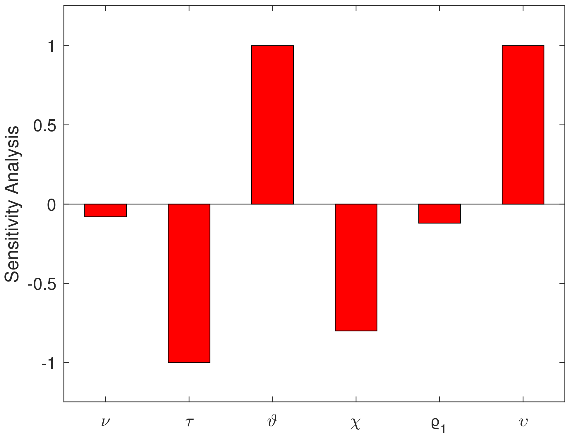
Figure 1. Plot of Sensitivity Analysis based on R 0 with each parameter associated with R 0 .
Fractalfract 07 00358 g001
Figure 2. The implementation of fractal-fractional orders with κ = 0.5 and λ = 0.5 can lead to optimal control of COVID-19. This is due to the influence of vaccination and treatment factors, represented by u 1 and u 2 , respectively.
Fractalfract 07 00358 g002
Figure 3. The dynamics of vaccine control variable u 1 for κ = 1 and λ = 1 .
Fractalfract 07 00358 g003
Figure 4. The kinetics of the human population that is susceptible to a given condition is being studied for a fractal order of κ = 0.5 and different fractional orders denoted by λ .
Fractalfract 07 00358 g004
Figure 5. Dynamics of Infected Human Population for Fractal Order κ = 0.5 and various Fractional Orders, λ .
Fractalfract 07 00358 g005
Figure 6. Dynamics of Quarantine Human Population for Fractal Order κ = 0.5 and various Fractional Orders, λ .
Fractalfract 07 00358 g006
Figure 7. Dynamics of Protected Human Population for Fractal Order κ = 0.5 and various Fractional Orders, λ .
Fractalfract 07 00358 g007
Figure 8. Dynamics of Deaths in Quarantine and Infected Human Populations for Fractal Order κ = 0.5 and various Fractional Orders, λ .
Fractalfract 07 00358 g008
Figure 9. Dynamics of Susceptible Human Populations for Fractional Order λ = 0.5 and various Fractal Orders, κ .
Fractalfract 07 00358 g009
Figure 10. Dynamics of Infected Human Populations for Fractional Order λ = 0.5 and various Fractal Orders, κ .
Fractalfract 07 00358 g010
Figure 11. Dynamics of Quarantine Human Populations for Fractional Order λ = 0.5 and various Fractal Orders, κ .
Fractalfract 07 00358 g011
Figure 12. Dynamics of Protected Human Populations for Fractional Order λ = 0.5 and various Fractal Orders, κ .
Fractalfract 07 00358 g012
Figure 13. Dynamics of Deaths in Quarantine and Infected Human Populations for Fractional Order λ = 0.5 and various Fractal Orders, κ .
Fractalfract 07 00358 g013
Figure 14. Dynamics of Susceptible Human Population for various Fractal-Fractional Orders.
Fractalfract 07 00358 g014
Figure 15. Dynamics of Infected Human Population for various Fractal-Fractional Orders.
Fractalfract 07 00358 g015
Figure 16. Dynamics of Quarantine Human Population for various Fractal-Fractional Orders.
Fractalfract 07 00358 g016
Figure 17. The study investigates the behavior of safeguarded human communities under different fractal-fractional orders.
Fractalfract 07 00358 g017
Figure 18. Dynamics of Deaths in Quarantine and Infected Human Populations for various Fractal-Fractional Orders.
Fractalfract 07 00358 g018
Figure 19. The study investigates the impact of the psychological effect parameter, ω , on the dynamics of the susceptible human population.
Fractalfract 07 00358 g019
Figure 20. This research examines the influence of the psychological factor parameter, ω , on the kinetics of the infected human population.
Fractalfract 07 00358 g020
Figure 21. The study investigates the behavior of protected population under different values of the psychological impact parameter, denoted as ω .
Fractalfract 07 00358 g021
Figure 22. Dynamics of Deaths in Quarantine and Infected Human Populations for various values of Parameter of Psychological Effect, ω .
Fractalfract 07 00358 g022
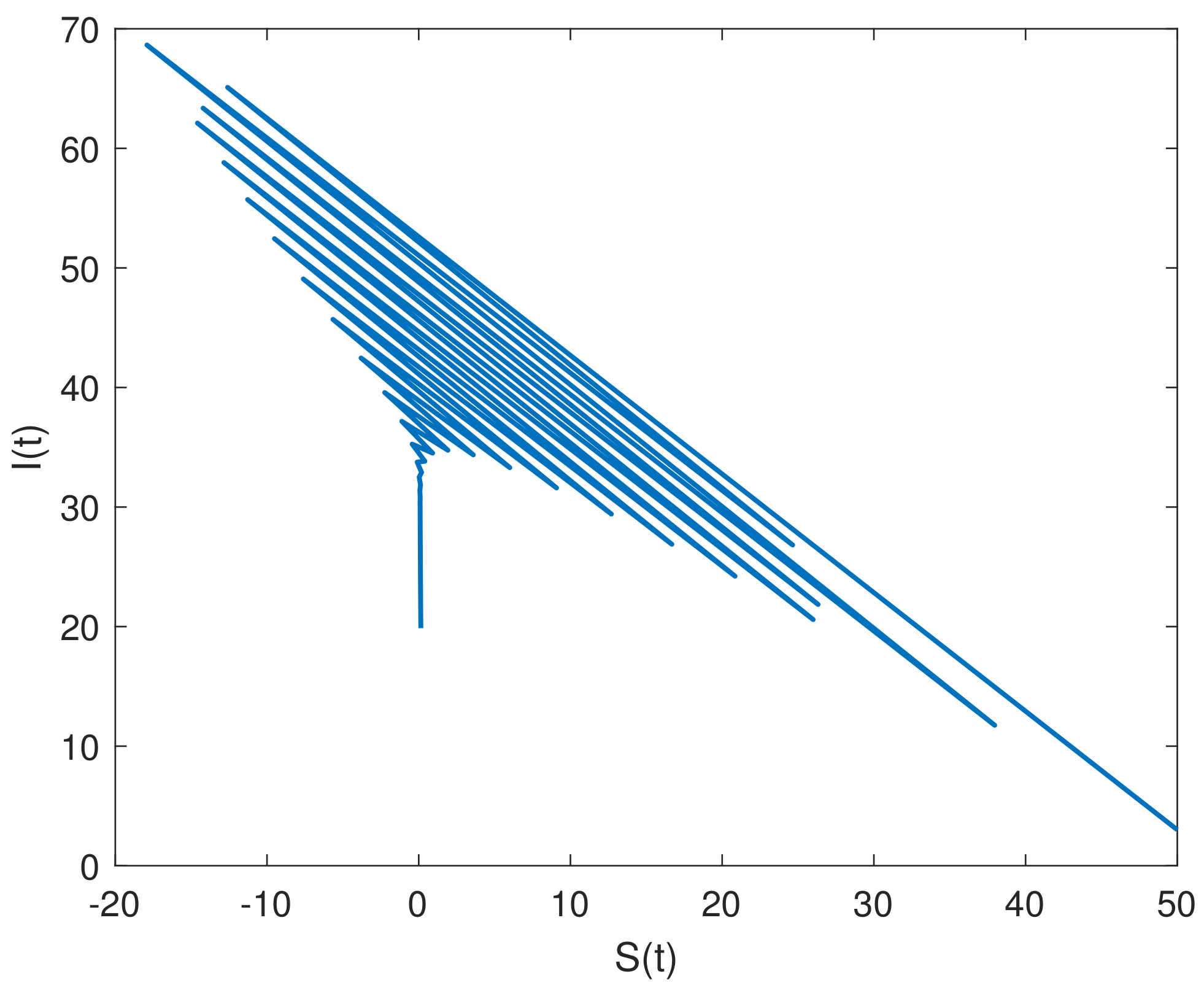
Figure 23. Phase Portraits of Susceptible Human vs. Infected Human Populations with Fractal–Fractional orders κ = 0.5 , and λ = 0.5 and with Initial condition larger than S ( 0 ) = 55 .
Fractalfract 07 00358 g023
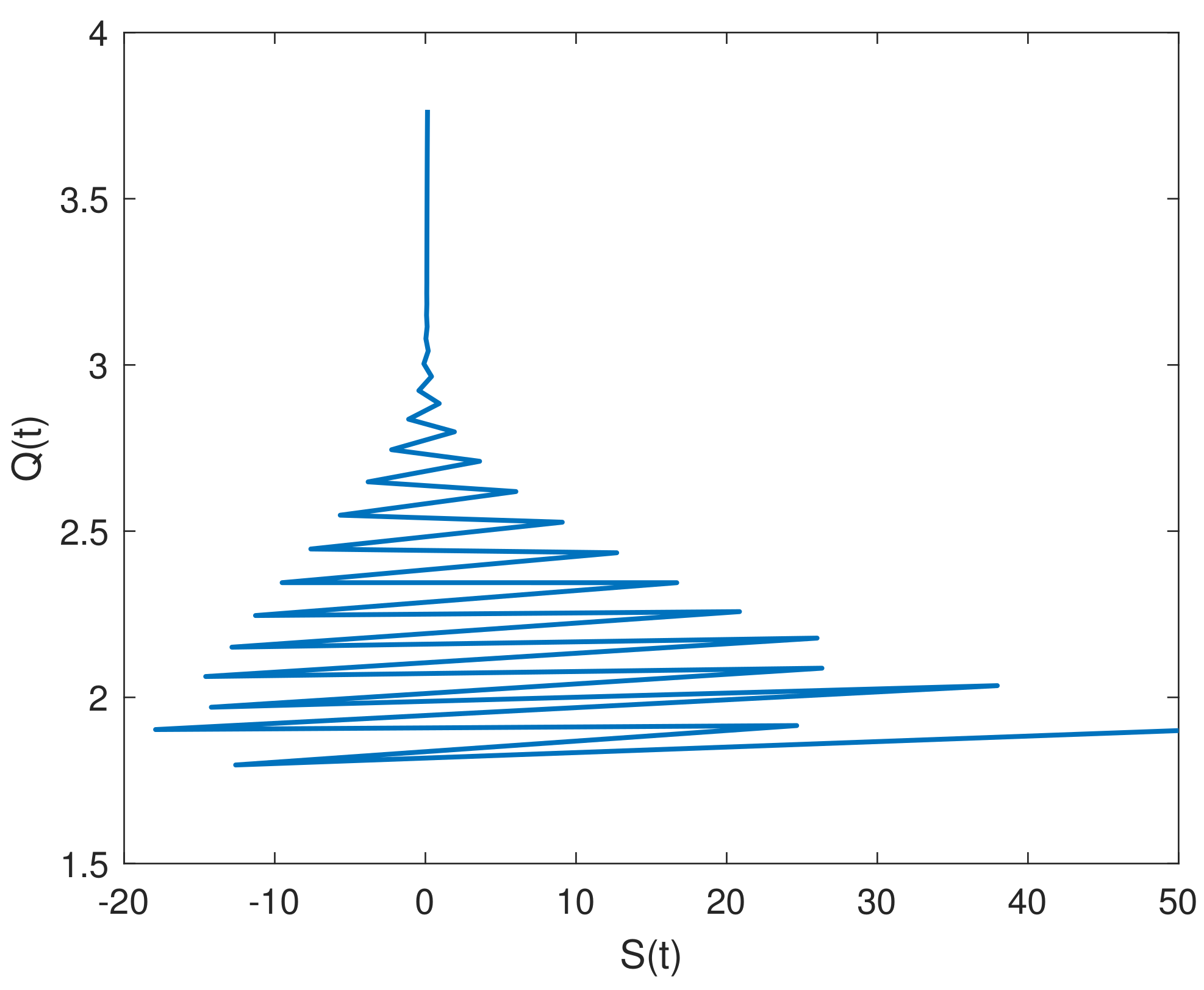
Figure 24. Phase Portraits of Susceptible Human vs. Quarantine Human Populations with Fractal-Fractional orders κ = 0.5 , and λ = 0.5 and with Initial condition larger than S ( 0 ) = 55 .
Fractalfract 07 00358 g024
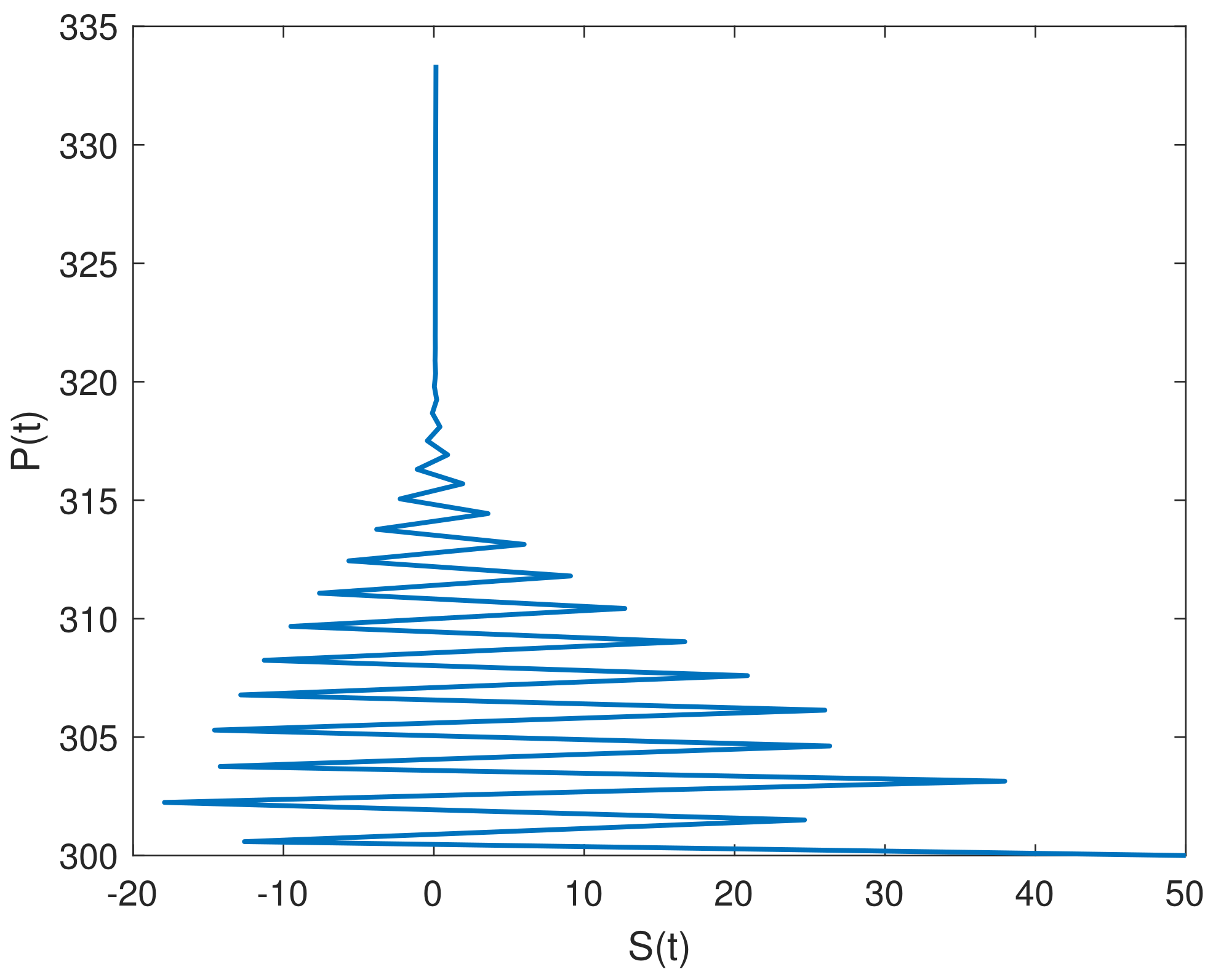
Figure 25. Phase Portraits of Susceptible Human vs. Protected Human Populations with Fractal-Fractional orders κ = 0.5 , and λ = 0.5 and with Initial condition larger than S ( 0 ) = 55 .
Fractalfract 07 00358 g025
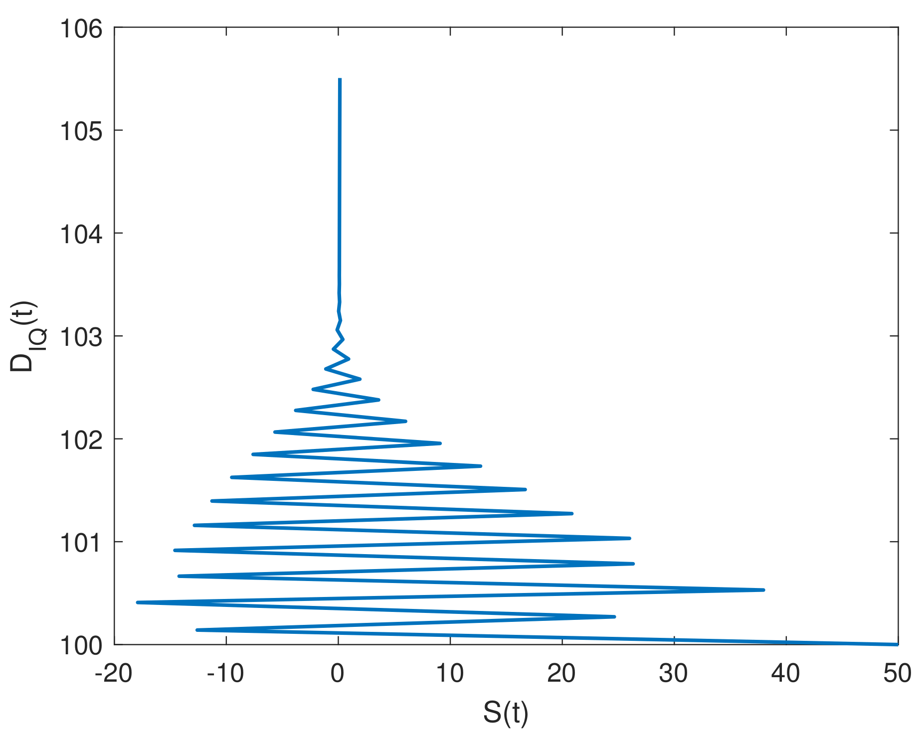
Figure 26. Phase Portraits of Susceptible Human vs. D Q I Human Populations with Fractal-Fractional orders κ = 0.5 , and λ = 0.5 and with Initial condition larger than S ( 0 ) = 55 .
Fractalfract 07 00358 g026
Figure 27. In this figure, we check for the stability of the solution of Susceptible Human Populations with Fractal-Fractional orders κ = 0.5 , and λ = 0.5 in which we experience the fluctuation with different initial conditions starting from S ( t = 0 ) = 30 and above. Light blue color nearly, green at S ( t = 0 ) = 10 , indigo color at S ( t = 0 ) = 20 , yellow at S ( t = 0 ) = 30 , red at S ( t = 0 ) = 40 , and dark blue at S ( t = 0 ) = 55 .
Fractalfract 07 00358 g027
Figure 28. Stability Curves of Infected Human Populations with Fractal-Fractional orders κ = 0.5 , and λ = 0.5 and with with various Initial conditions in which the Initial conditions larger than I ( 0 ) = 50 starts fluctuation.
Fractalfract 07 00358 g028
Figure 29. Stability Curves of Quarantine Human Populations with Fractal-Fractional orders κ = 0.5 , and λ = 0.5 and with with various Initial conditions.
Fractalfract 07 00358 g029
Figure 30. Stability Curves of Protected Human Populations with Fractal-Fractional orders κ = 0.5 , and λ = 0.5 and with with various Initial conditions.
Fractalfract 07 00358 g030
Figure 31. Stability Curves of D Q I Human Populations with Fractal-Fractional orders κ = 0.5 , and λ = 0.5 and with with various Initial conditions.
Fractalfract 07 00358 g031
Figure 32. The dynamics of treatment control variable u 2 for κ = 1 and λ = 1 .
Fractalfract 07 00358 g032
Figure 33. The 3D dynamics of R 0 with parameters ϑ and υ associated with its contour plot.
Fractalfract 07 00358 g033
Figure 34. The 3D dynamics of R 0 with parameters ϑ and τ associated with its contour plot.
Fractalfract 07 00358 g034
Figure 35. The 3D dynamics of R 0 with parameters ϑ and χ associated with its contour plot.
Fractalfract 07 00358 g035
Figure 36. The 3D dynamics of R 0 with parameters ϑ and ν associated with its contour plot.
Fractalfract 07 00358 g036
Figure 37. The 3D dynamics of R 0 with parameters ϑ and ϱ 1 associated with its contour plot.
Fractalfract 07 00358 g037
Table 1. A tabular representation of the demographic subgroups with their respective Initial coditions.
SymbolDescription of Compartment/ClassInitial Conditions
S ( t ) Susceptible Human Population0.85
I ( t ) Exposed Human Population3
Q ( t ) Infected Human Population1.9
P ( t ) Recovered Human Population300
D I Q ( t ) Susceptible Vector Population100
Table 2. A tabular representation of the value of Parameters and description.
SymbolDescription of ParameterValue
υ Recruitment Rate [13]. τ × N ( 0 )
τ Natural Death Rate [13]. 1 67.7 × 365
ϑ Transmission rate.0.2784
ω Psychological Effect on Humans [14].[0,1]
χ Recovery Rate of Infected Population [15].0.1
ϖ Recovery Rate of Quarantine Population.0.020
ν Incubation Period.0.010
ϱ 1 The mortality rate of the afflicted populace as a result of a pathological condition.0.015
ϱ 2 Mortality rate among individuals subjected to quarantine as a result of disease.0.015
Table 3. Sensitivity of the R 0 versus proposed parameters.
ParameterSensitivity IndexValueParameterSensitivity IndexValue
ν s ν R 0 −0.0799 τ s τ R 0 −1.0003
ϑ s ϑ R 0 1 χ s χ R 0 −0.7997
ϱ 1 s ϱ 1 R 0 −0.1199 υ s υ R 0 1
Disclaimer/Publisher’s Note: The statements, opinions and data contained in all publications are solely those of the individual author(s) and contributor(s) and not of MDPI and/or the editor(s). MDPI and/or the editor(s) disclaim responsibility for any injury to people or property resulting from any ideas, methods, instructions or products referred to in the content.