Fractal Analysis and FEM Assessment of Soft Tissue Affected by Fibrosis

Abstract

This research shows an image processing method to determine the liver tissue’s mechanical behavior under physiological damage caused by fibrosis pathology. The proposed method consists of using a liver tissue CAD/CAE model obtained from a tomography of the human abdomen, where the diaphragmatic surface of this tissue is compressed by a moving flat surface. For this work, two tools were created—the first to analyze the deformations and the second to analyze the displacements of the liver tissue. Gibbon and MATLAB^® were used for numerical analysis with the FEBio computer program. Although deformation in the scenario can be treated as an orthogonal coordinate system, the relationship between the total change in height (measured) and the deformation was obtained. The outcomes show liver tissue behavior as a hyperelastic model; the Mooney–Rivlin mathematical characterization model was proposed in this case. Another method to determine the level of physiological damage caused by fibrosis is fractal analysis. This work used the Hausdorff fractal dimension (HFD) method to calculate and analyze the 2D topological surface.

1. Introduction

Tissues are essential elements in all living beings, and their composition and structure play a fundamental role in their biological and mechanical behavior. The literature shows that tissues mainly comprise collagen fibers and elastin, forming interlocking structures. Additionally, tissues are coated with a layer of proteoglycans, which works as a specific protective function [1].

The interaction between the biology and mechanical behavior of tissues generally depends on their internal organization, mainly when they exhibit anisotropic behavior. For instance, liver tissue displays this anisotropic property, visually evident through the wavy pattern of collagen fibers [2]. Another highlighted aspect of liver tissue is its structural composition, with approximately 80% being water, making it an incompressible material [3].

Therefore, when analyzing the mechanical behavior of liver tissue under loads, it is essential to adapt equilibrium equations for its incompressibility and ensure coherence with the load system and internally generated stresses [4,5]. There is a limitation in finding a solution because the relationship between stresses and deformations in biological tissues is unknown. This leads to a hyperelastic model applied to liver tissue [6,7,8]. Liver fibrosis pathology results from various factors, such as metabolic disorders, viral causes, alcoholism, drugs, and congenital anomalies. This condition is associated with a sustained inflammatory process that leads to scar tissue formation, affecting the liver tissue’s vital function and increasing its stiffness. It is crucial to emphasize that liver fibrosis is a chronic condition, unlike acute diseases, and its diagnosis and treatment have increased significantly due to the possibility of preventing and treating some causative factors [9,10].

In recent years, more detailed analysis of liver tissue has been conducted using constitutive models and the finite element method, along with the application of autonomous learning algorithms [11,12]. For example, Edoardo Mazza proposed Constitutive Modeling of Human Liver Based on in Vivo Measurements using in vivo aspiration experiments on human livers to determine the properties of a nonlinear viscoelastic constitutive model. This approach enabled the prediction of nonlinear and time-dependent behaviors [13]. Another study by Jessica L. Sparks focused on Constitutive Modeling of Rate-Dependent Stress-Strain Behavior of Human Liver in Blunt Impact Loading. The researchers adapted a constitutive model to understand hepatic behavior under high-strain-rate loading by applying polymer mechanics concepts.

Additionally, Stéphanie Marchesseau presented a Porous Hyperelastic Viscous Model to Represent Hepatic Parenchyma, emphasizing the significance of visco-hyperelasticity obtained through the Prony series and the use of linear Darcy’s law to simulate hepatic perfusion. Relative effects of the liver model’s hyperelastic, viscous, and porous components were compared with rheological experiments [14,15]. Furthermore, the research by Zhan Gao on Constitutive Modeling of Liver Tissue: Experiment and Theory has made significant advancements in real-time surgical simulations, applying complex nonlinear constitutive models to biological tissues, resulting in haptic and graphic precision [16].

On the other hand, in the literature, fractals are defined as geometric objects with similarities across different scales. Fractal geometry, proposed by mathematician Benoit Mandelbrot, has been employed to describe and study fractals, including the Mandelbrot, set as a mathematical representation in the complex plane [17]. A fractal object is one whose fractal dimension (FD) is generally but not always a fractional number that is larger than its topological dimension (TD) and smaller than its embedment dimension (ED), such that $TD<FD<ED$, where FD can be defined as a measure of the complexity or roughness of this kind of shape and can be treated as the degree to which a set “fills” the Euclidean space in which it is embedded. In various scientific fields, such as biomedicine, materials analysis, environmental sciences, and computer graphics, among others, the usefulness of fractal dimension as a structural descriptor has been demonstrated [18,19,20,21,22].

Table 1. Comparison of liver tissue analysis methods.

	Advantages	Disadvantages
Autonomous learning algorithms	Adaptability to different types of biological tissues and problems; Ability to discover patterns and nonlinear relationships in data.	Requires large amounts of training data; Interpretability of the results; Possible overfit in training.
FEM	Different types of biological tissue applications; With the proper settings, the FEM can provide precise and detailed results on the mechanical behavior of tissues.	FEM simulations can require a significant amount of computational resources; In some cases, simplifications in the constitutive model may be required due to the complexity and amount of data needed.

compares the advantages and disadvantages of the analysis methods used for liver tissue. However, for this study, an integrative approach was sought. For this reason, this article presents an approach that combines fractal analysis with the finite element method to assess the mechanical properties of fibrosis-affected liver tissue. This integration of approaches enhances our understanding of the evolution of liver fibrosis and its effects on tissue mechanical properties, with significant implications for diagnosing and treating this disease. This multidisciplinary research aims to contribute to the scientific knowledge showing new perspectives for developing more precise and effective therapeutic strategies for patients with liver fibrosis.

2. Materials and Methods

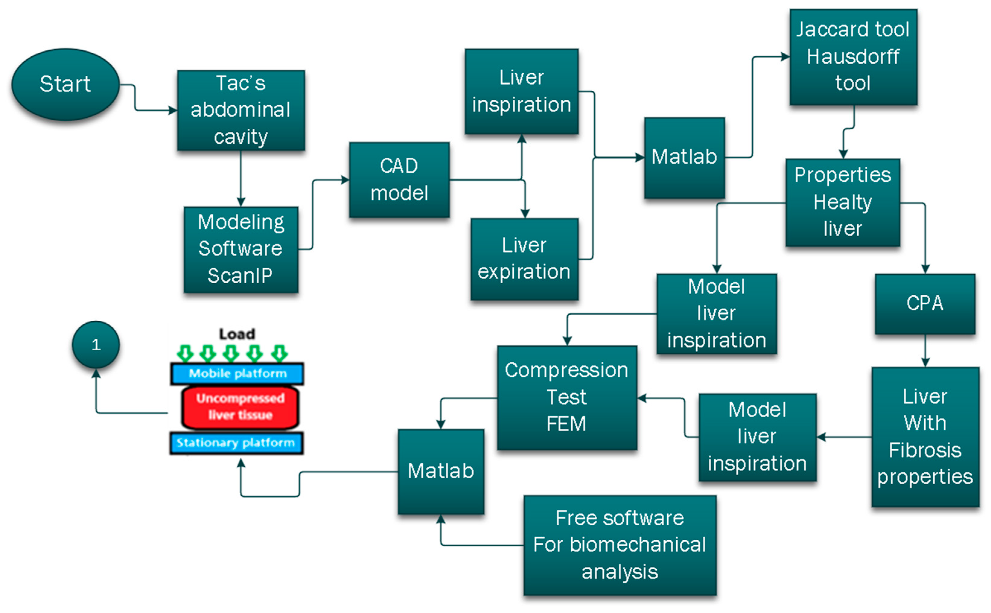
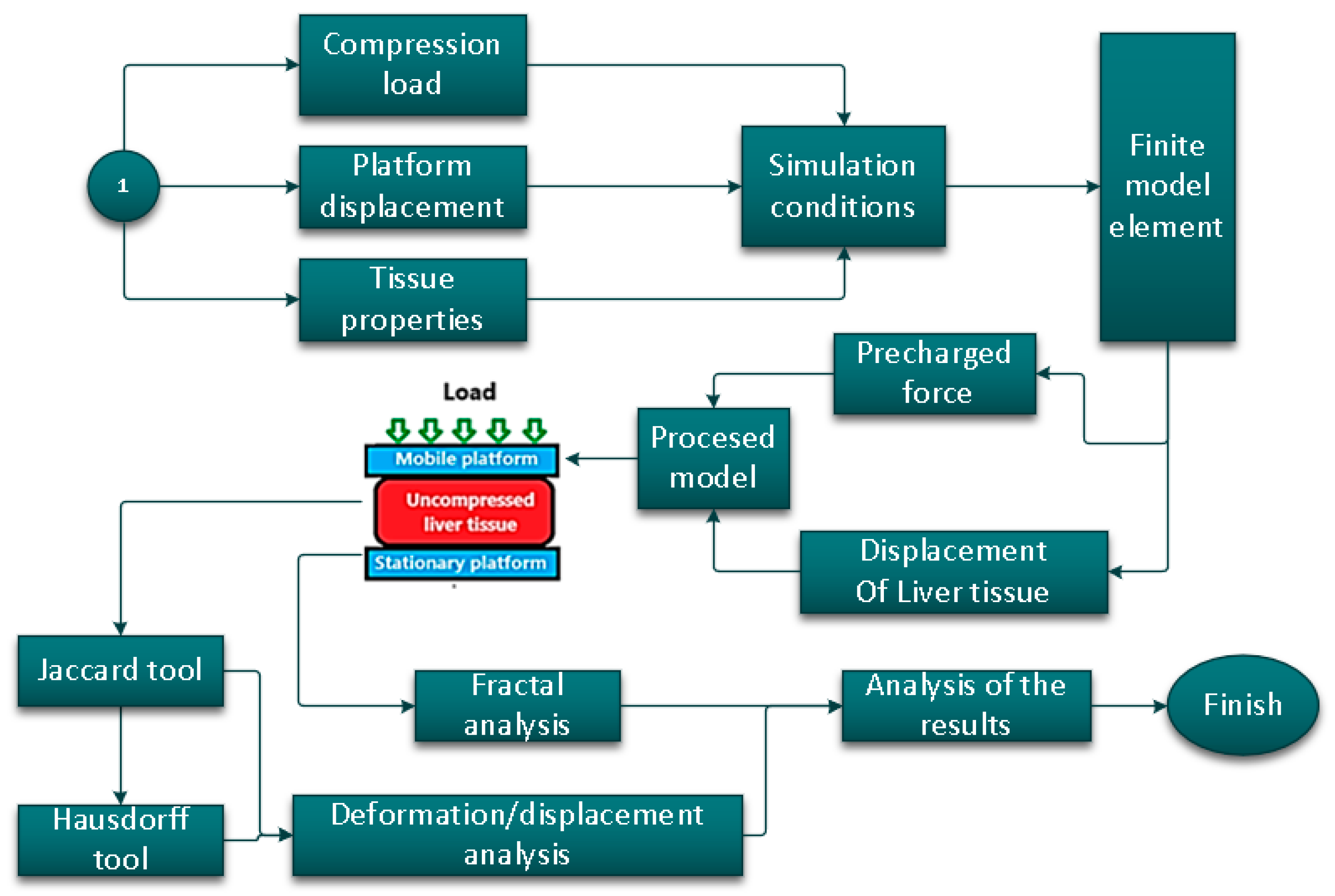
This work proposes a methodology to analyze liver tissue’s mechanical behavior under a compressive load by a finite element method and the analysis of the results using tools for image processing; this methodology is visualized in Figure 1 and Figure 2. Reconstructing a liver tissue computer-aided design/computer-aided engineering (CAD/CAE) model to accurately represent the mechanical behavior of natural liver tissue affected by fibrosis can be complex [23,24,25,26,27,28].

However, it is achievable with careful consideration of certain factors.

Material Properties: Accurate representation of liver tissue behavior requires appropriate material properties. For fibrosis-affected liver tissue, the mechanical properties will be different from healthy tissue. Experimental data or literature-based values for the mechanical properties of fibrotic liver tissue should be used to calibrate the model. Constitutive Model: Choosing an appropriate constitutive model is crucial for accurately representing mechanical behavior. The model should adapt for fibrotic liver tissue’s nonlinear, anisotropic, and viscoelastic nature. Specialized models, such as hyperelastic or viscoelastic models with anisotropic properties, may be used. Microstructure and Anisotropy: Liver tissue exhibits anisotropic behavior due to its hierarchical microstructure. The CAD/CAE model should incorporate this anisotropy and other constituents in the fibrotic tissue. Boundary Conditions: Properly defining the boundary conditions is essential for realistic simulation. The model should be subjected to loading conditions that mimic real-world scenarios, such as compressive loads or shear forces experienced by the liver.

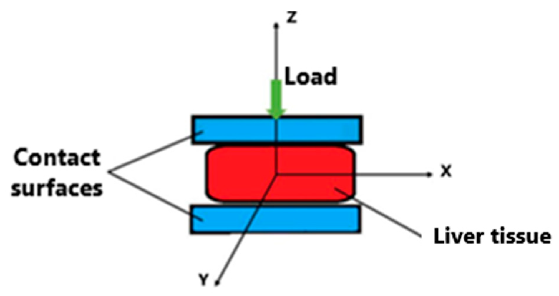
Multi-Scale Approach: Liver tissue mechanics involve interactions at multiple scales, from the microstructural to the organ level. A multi-scale modeling approach helps capture fibrotic liver tissue’s complex mechanical behavior. A 32-year-old adult provided the tomographies used in this study and belonging to the abdominal cavity. It is worth noting that the tomographies were taken during the respiratory cycle, specifically during inspiration and expiration. The analysis scenario included two platforms, one mobile and one fixed, as shown in Figure 2. The objective of the mobile platform was to generate a compression load similar to the maximum contractile force that the diaphragm generates during the respiratory cycle. The numerical simulation was conducted in MATLAB^® version R2019a is a software application developed by MathWorks, a company based in Natick, Massachusetts, USA. Using a biomechanical analysis plugin called Gibboncode. This plugin works with the software FEBio version 3.7.0, developed by Musculoskeletal Research Laboratories at the University of Utah and at the Musculoskeletal Biomechanics Laboratory at Columbia University, where the numerical simulation is performed using the finite element method. For this study, the hyperelastic Mooney–Rivlin model was used. The results were analyzed using the Jaccard index for deformations and the Hausdorff distance for displacements. The analysis concluded by applying fractal analysis to study the surface roughness of the hepatic tissue.

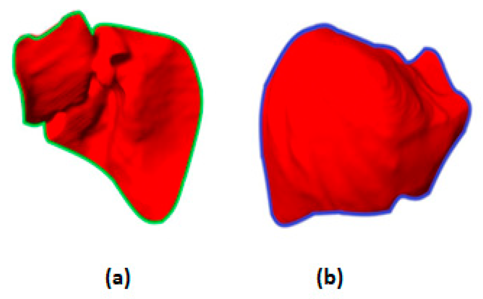
The liver tissue was divided into two study cases, as shown in Figure 3. This study applied a compression test only to liver tissue without considering the surrounding tissues. The first case study consisted of a numerical simulation using liver tissue reconstructed by tomography. This tissue was in a healthy condition, and a compression load was applied through a mobile platform on the diaphragmatic surface of the tissue. The second case study was a numerical simulation of the three-dimensional liver tissue model with properties of physiological damage caused by the pathology of liver fibrosis. Similarly, a compressive load was applied to the diaphragmatic surface of the tissue. Therefore, the model had two boundary conditions; the tissues close to the liver tissue’s visceral surface generated the compression forces. Thus, the homogeneous conditions (support nodes) were the entire visceral surface. On the other hand, for the diaphragmatic surface, the entire diaphragmatic surface was taken as non-homogeneous boundary conditions (displacement nodes).

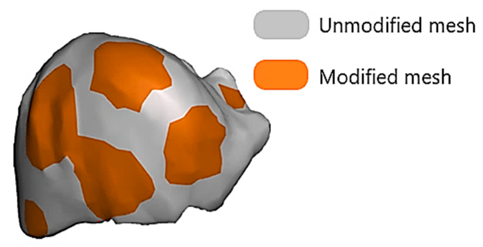
The border conditions in the second case study were where the liver tissue presented liver fibrosis. A compression force was generated by the tissues close to the visceral surface. The hepatic tissue’s three-dimensional model was used without any alteration in its structure due to physiological processes. The second case study was modified to simulate the deterioration of advanced fibrosis in different areas of the tissue structure.

The mesh size is a factor that influences the system’s stiffness, as visualized in Figure 4.

The analysis was performed with an image-based geometry and bioengineering plugin, an open-source MATLAB^® toolbox that includes a variety of image, geometry visualization, and processing tools. It is interconnected with open-license software for creating a robust tetrahedral mesh. This combination provided a highly flexible image-based or modeling environment and enabled advanced finite element analysis. The contact surfaces generated compression on the diaphragmatic surface of the liver tissue. It was essential to establish the contact conditions because if the numerical analysis processor was not performed, it would not interpret which surface suffered the displacements in its geometry or which geometry generated the force.

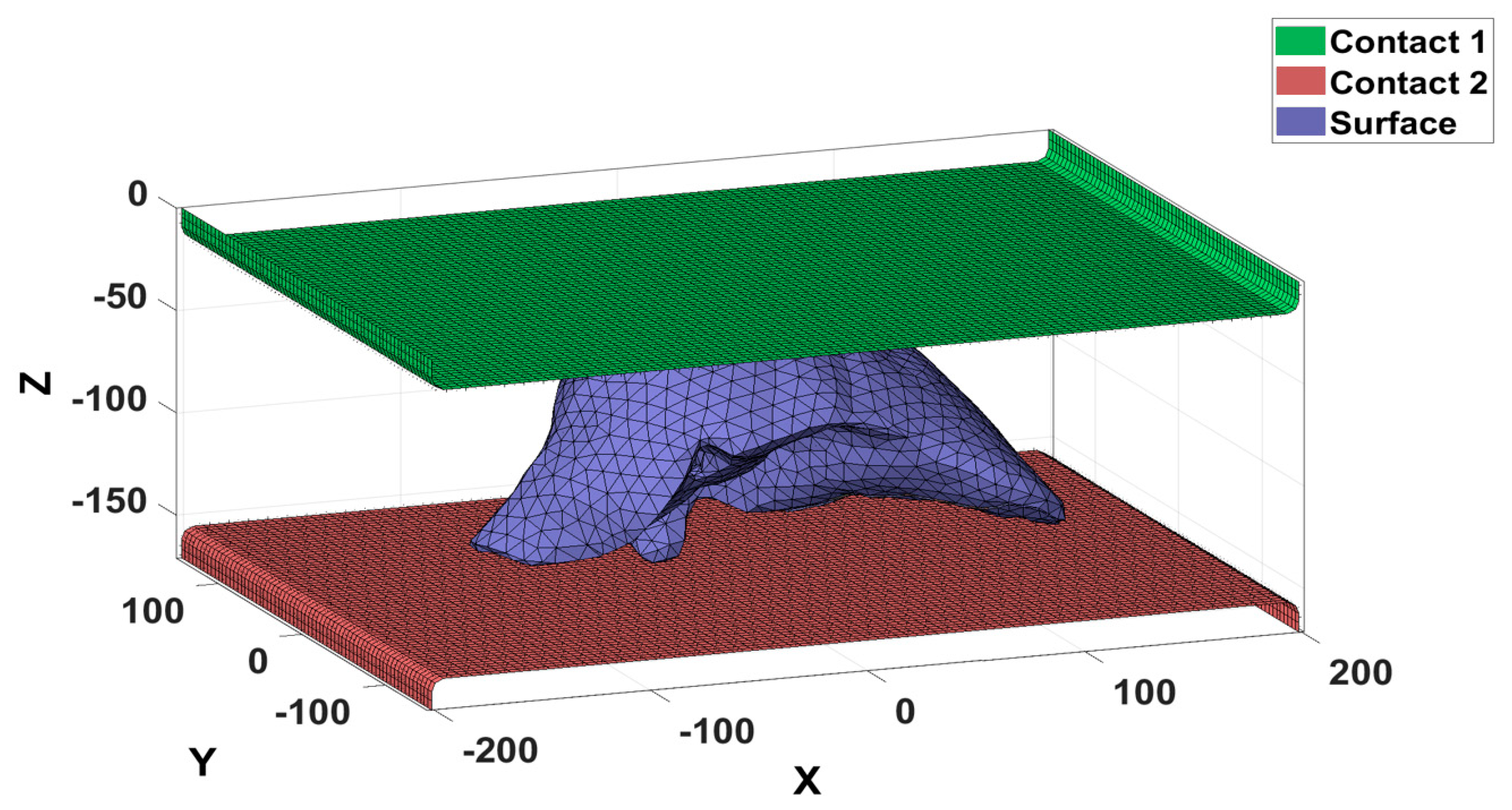
The first type of contact was related to the flat surfaces that exerted compression on the diaphragmatic area of the liver tissue. It was subdivided into Master Contact Surface 1 and Master Contact Surface 2. Master Contact Surface 1 moved 34 mm during the analysis, and Master Contact Surface 2 remained fixed during the analysis. The second type of contact was directly related to the three-dimensional liver tissue model because it was deformed and, therefore, was called the slave contact surface. The visualization of the contact surfaces is shown in Figure 5.

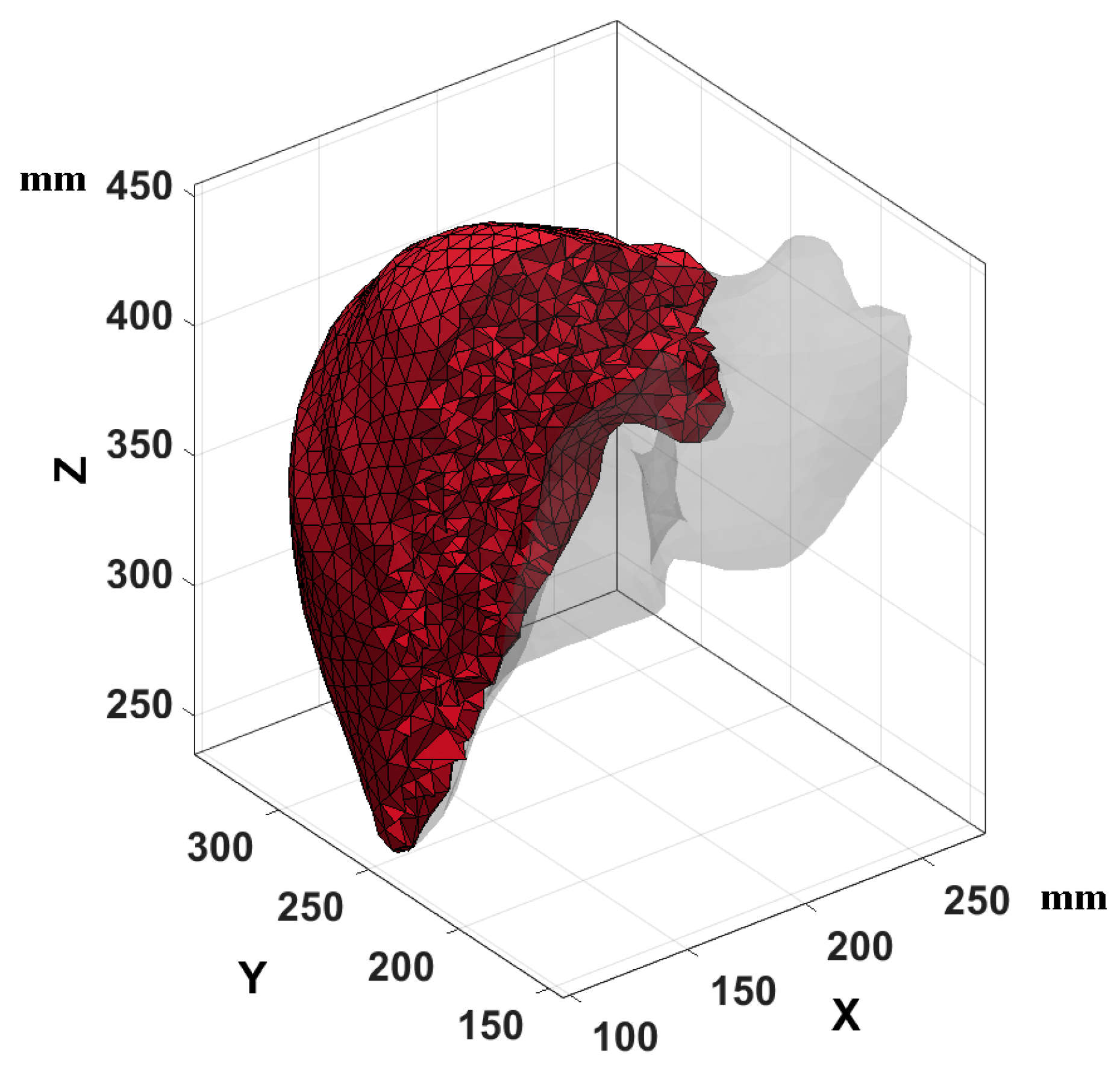
A tetrahedral mesh was used; this mesh provides satisfactory results for irregular surfaces such as liver tissue because this type of irregular surface is standard for a visceral surface. These surfaces are compressed by the organs surrounding this tissue due to natural processes in the human body. The STL liver tissue model had 1569 nodes before being re-meshed for tetrahedral mesh schemes. The three-dimensional model provided a surface geometry. The surface data were processed in a triangulated way. For both study cases, regular tetrahedral mesh was established, and the desired volume was specified to estimate the volume given by the input surface. The mesh was created with MATLAB^® version R2019a (software application developed by MathWorks, Natick, MA, USA) with the characteristics of 19,493 nodes and 35,982 tetrahedrons. Figure 6 shows the tetrahedral mesh applied in the three-dimensional liver tissue model.

The next step was to analyze the results using two image processing tools. Two different methods were applied to analyze the deformations in the diaphragmatic surface of the liver tissue. The displacements of the liver tissue, the stress, the Jaccard coefficient, and the Hausdorff distance using a code in MATLAB^® were implemented. Two groups of binary data were necessary to implement the Jaccard similarity coefficient for artificial vision. It was necessary to segment the images of interest, convert them into binary images, and apply the Jaccard coefficient. The hue saturation value (HSV) filter generated accurate binary images without losing image details because this filter limits the luminescence of the colors that make up the image, in contrast to other filters. Moreover, binary images have only two possible grey levels and are rendered using only 1 bit per pixel, so it is enough to transform the segmented image to grayscale.

The code implemented in MATLAB^® consists of a series of instructions. The first is to insert the images in RGB format. In the second step, the images based on an HSV filter are segmented using channels to separate the luminosity of the colors. The third step transforms the segmented images into binary data, and finally, the code compares the binary data of the registered images based on Jaccard’s criteria. The code overlaps both images and displays a window showing a similar result as the applied filters.

The Hausdorff algorithm defines the displacement distance. The liver tissue without deformation was set as “A”, and the deformed tissue was set as “B”. Then, the code of the Hausdorff distance seeks the distance of the sets to find the maximum distance between the arrays. A group of transformations was applied to a set of points from group “A” to “B”. In this way, more than 90% of the points in “A” and “B” had the same distance.

Before starting the analysis by the finite element method, it was necessary to determine the properties of the liver tissue in healthy conditions. In this case, these were obtained during the respiratory cycle, where the lungs expand, and consequently, the diaphragm undergoes a contraction to expand the lungs within the rib cage. Consequently, the diaphragm contraction compresses and generates considerable deformations on the tissue surface.

The diaphragm performs a role in the respiratory cycle in the expansion of the lungs. Consequently, the diaphragm contracts with the auxiliary muscles, generating deformations in the liver tissue. This action is caused by the maximum contractile force that occurs when a contraction begins from an optimal resting length of the diaphragm and when the diaphragm is restricted to contracting isometrically [29].

The mechanical properties of the liver tissue affected by fibrosis were assessed based on the collagen proportional area (CPA). The relationship with the percentage of collagen in the liver tissue affected by fibrosis is because the inflamed liver cells migrate through the endothelium of the portal vessels. The percentages of the proportional area of collagen were taken from a study called An analysis of intrinsic variations of low-frequency shear wave speed in a stochastic tissue model: the first application for staging liver fibrosis, prepared by the author Yu Wang. The collagen concentrations are shown in

Table 2. CPA concentrations of liver tissue affected by fibrosis.

Fibrosis Level	F0	F1	F2	F3	F4
Collagen proportional area (CPA)	9.67%	15.9%	16.68%	20.73%	32.67%

[30].

For this research, only the collagen concentration was considered for level F4 fibrosis. The properties were calculated approximately as the proportionality of the properties calculated for healthy liver tissue and the percentages of collagen between healthy conditions (F0) and with fibrosis (F4). The hyperelastic response of liver tissue was used to determine the elastic energy stored by a unit of volume, the stiffness present in the tissue, and the behavior of stresses and deformations. Collagen is one of the most common proteins in tissues because it is considered a structural element of soft tissues. In addition, collagen provides specific mechanical properties, such as stiffness, elasticity, and anisotropy. The Mooney–Rivlin model was used. Figure 7 shows the coordinate system used to make the proposed mathematical measurements.

The method of obtaining the fractals was divided into three steps, described below. The first step was to convert the RGB input into a grayscale image. To obtain a binary image, it was necessary to take into consideration that an RGB input image converted to grayscale I can be treated as a two-dimensional function that we named I(x,y), where I(x,y)∈ {0, 1,⋯, n_1-1}. I(x,y) is assigned pixel intensity in the (x,y) directions. Before carrying out the process of obtaining the vector that contained the characteristics of the image, the binary decomposition technique [32] was used. This lop technique decompensates the image in grayscale by applying thresholding processes [33,34].

$$I_b\left(x, y; t\right)=\left\{\begin{array}{c}1 if I\left(x, y\right)\ge t \\ 0, otherwise\end{array}\right.$$

(1)

There are different methods of fractal geometry to determine the fractional dimensions, but the most used one is based on the Hausdorff dimension. For this method, it must be considered that the object of study has a Euclidean dimension $E$. The fractal dimension of Hausdorff $D_0$ is represented by the scaling relation given in Equation (2):

$$D_0=\frac{log N\left(ϵ\right) }{log {ϵ}^{-1} }$$

(2)

where $N\left(ϵ\right)$ is the count of boxes with dimension $E$ that the object uses. If an object is taken in its form from a binary image, it is possible to obtain the Hausdorff fractal dimension using the box-counting algorithm. For this work, the algorithm was applied to a 2D case. As a first step, the image was divided into a grid. The next step was to calculate the $N\left(ϵ\right)$ of squares of $\in \times \in$ size that contained at least one pixel from the edge of the object under study.

3. Results

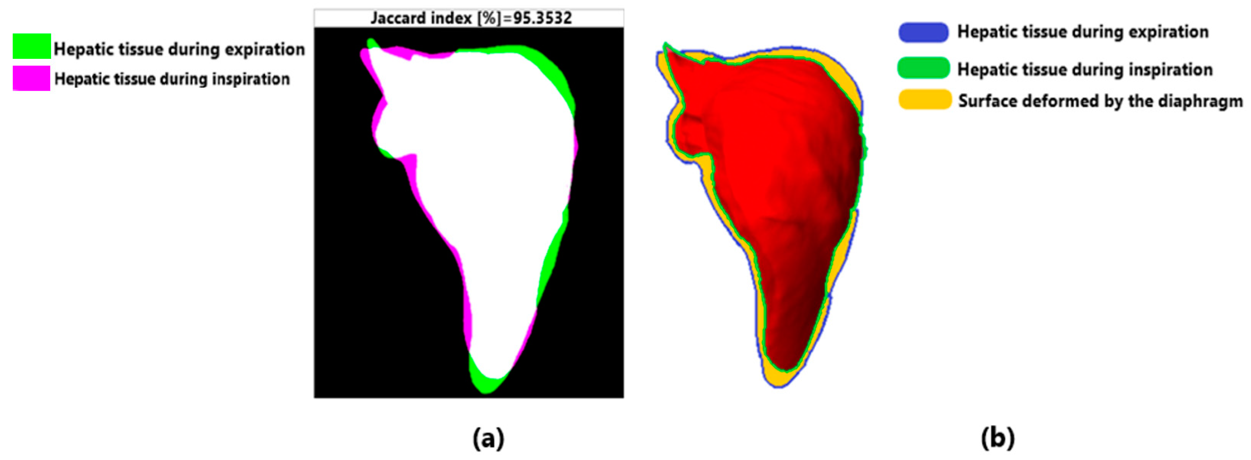
Before carrying out the numerical analysis with the previously proposed scenario, it was necessary to obtain the properties of the tissue for the first case study that corresponded to the healthy tissue. Later, they were determined for the second case study. It was necessary to use the image processing tool to define the properties, for which the Jaccard coefficient was implemented to establish the percentage of deformation in the diaphragmatic surface of the liver tissue to determine the type of behavior it presents as a material. The Jaccard index calculated the proportions of common elements among the sets concerning the total number of elements in both sets. This tool used binary images extracted from the liver tissue model as a point of comparison that was later transformed into matrices, and from these, the dissimilarities in percentages were compared. Figure 8 shows that the liver tissue during the respiratory cycle had a similarity of 95.35%, which means that the tissue underwent a deformation of 4.64%. Based on the results of the deformation, the liver tissue was considered with linear properties during the respiratory cycle.

The properties of healthy tissue were determined with classical mechanics. In the first instance, Young’s modulus was calculated as the stress ($\sigma$) caused by the force exerted on the lungs and the diaphragm during the respiratory cycle.

The maximum contractile force of the diaphragm exerted on the liver tissue used is shown in Figure 8. The area was obtained from the three-dimensional model of the tissue in inspiration using the lateral view. The maximum contractile force of the diaphragm during inspiration in a healthy person is approximately $1.26\frac{\mathrm{Kg}}{{\mathrm{cm}}^2}$. In this case, the contractile force was opposed because the diaphragm compressed the liver tissue, and the area of liver tissue under study was $110,993.59735 {\mathrm{mm}}^2.$ With these data, the stress produced on the surface was calculated as $\sigma =-111.3217439 Pa$. 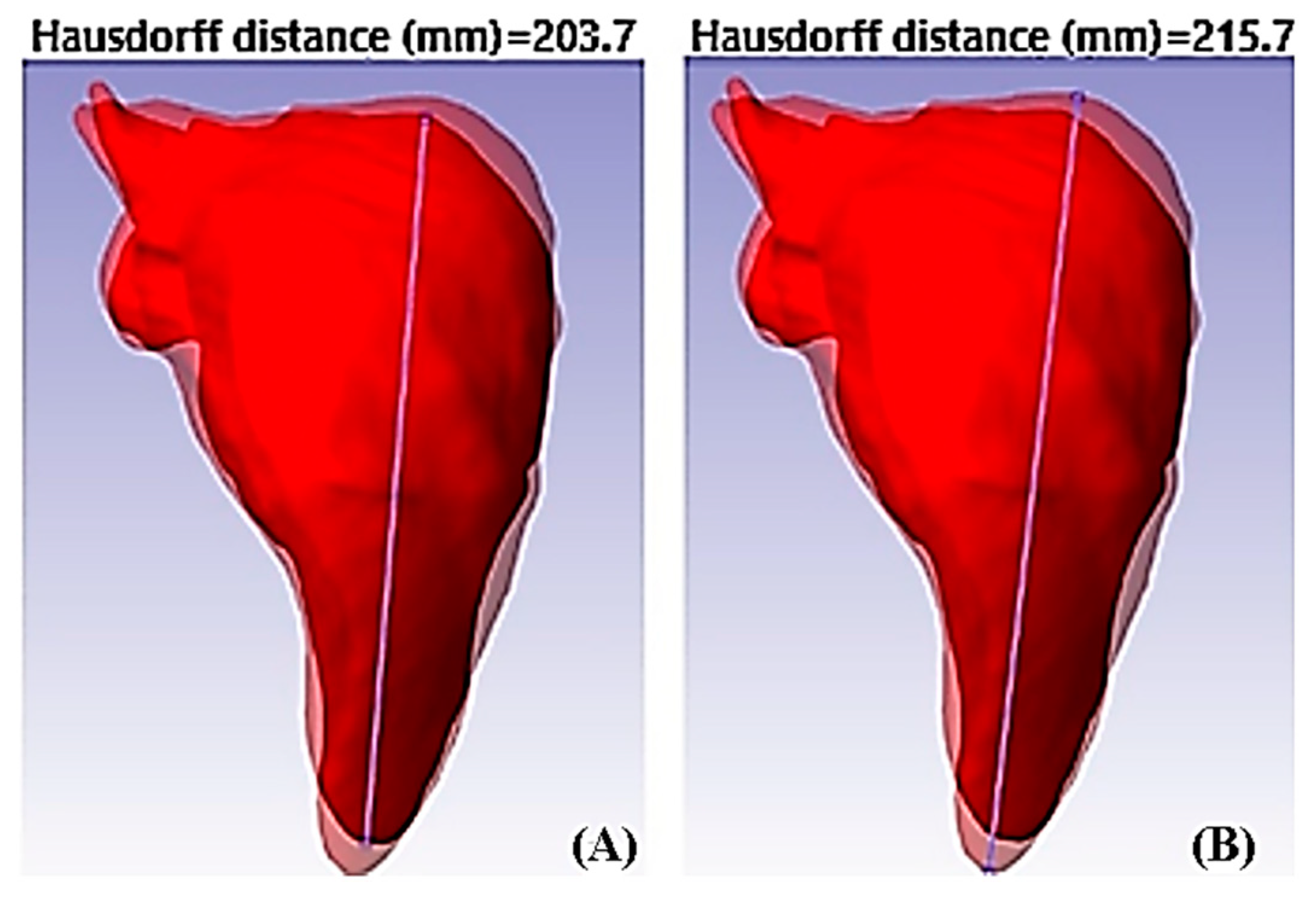After the deformation was determined ($\epsilon$), it was calculated from the three-dimensional models to determine the displacements of the liver tissue. The image processing using the Hausdorff distance took the lateral view of the liver tissue in .jpg image format, and MATLAB^® was overlaid, as shown in Figure 9. The deformations suffered by the liver tissue under normal conditions during the respiratory cycle are evident.

The Hausdorff distance quantifies the similarity or dissimilarity between two sets of points or geometric sets in a metric space. The Hausdorff distance in this work determined the displacements during the numerical analysis. The operation of this tool was necessary to extract RGB images from the liver tissue model, and the code binarized them to find the contours of the liver tissue model using the Canny method. The program determined the maximum and minimum points by obtaining the contours. From the points found, the minimum ones were discarded, and we only focused on the maximum point, expressed in pixels, and therefore, it had to be calculated in metric units. The Hausdorff distance calculation started from the superposition of the images belonging to the liver tissue during the respiratory cycle. After segmentation was carried out from the coordinates of both images, the liver tissue was extracted, subsequently determining the distances of the coordinates of the points extracted from the images contained in the specified search area until the maximum distance was found.

The displacements obtained were very considerable. The model in inspiration showed an enlargement of 6.54% compared to the model in expiration during the respiratory cycle. With the previous data, the unit deformation was calculated. We obtained a unit deformation of $\epsilon =-0.055632$.

Young’s modulus was determined based on the data obtained using computer tools. The module obtained was $E=2016.9174 Pa$. The next mechanic property to calculate was Poisson’s ratio ($v$). It was necessary to determine the strain and the transverse deformation. The Hausdorff distance calculated the transverse deformation. The images were superimposed with the displacements, as shown in Figure 10.

The transverse deformation and the displacements of the transverse strain was obtained as ${\epsilon }_T=0.026148$. Taking the strain and the transverse strain, finally, an approximation of Poisson’s modulus of the liver tissue in the respiratory cycle was determined with the data obtained from the image processing. The Poisson’s modulus obtained was $\upsilon =0.470$. Another property necessary for numerical simulation was the volumetric modules. The volumetric modulus was calculated based on its relationship with Young’s and Poisson’s modulus. The volumetric modulus obtained was as follows: $K=11,205.09667 Pa$. The last parameter to be calculated for healthy tissue was the stiffness modulus. The stiffness obtained indicates that liver tissue in healthy conditions was a soft material. Little force was needed to deform it, with $G=686.026 Pa$.

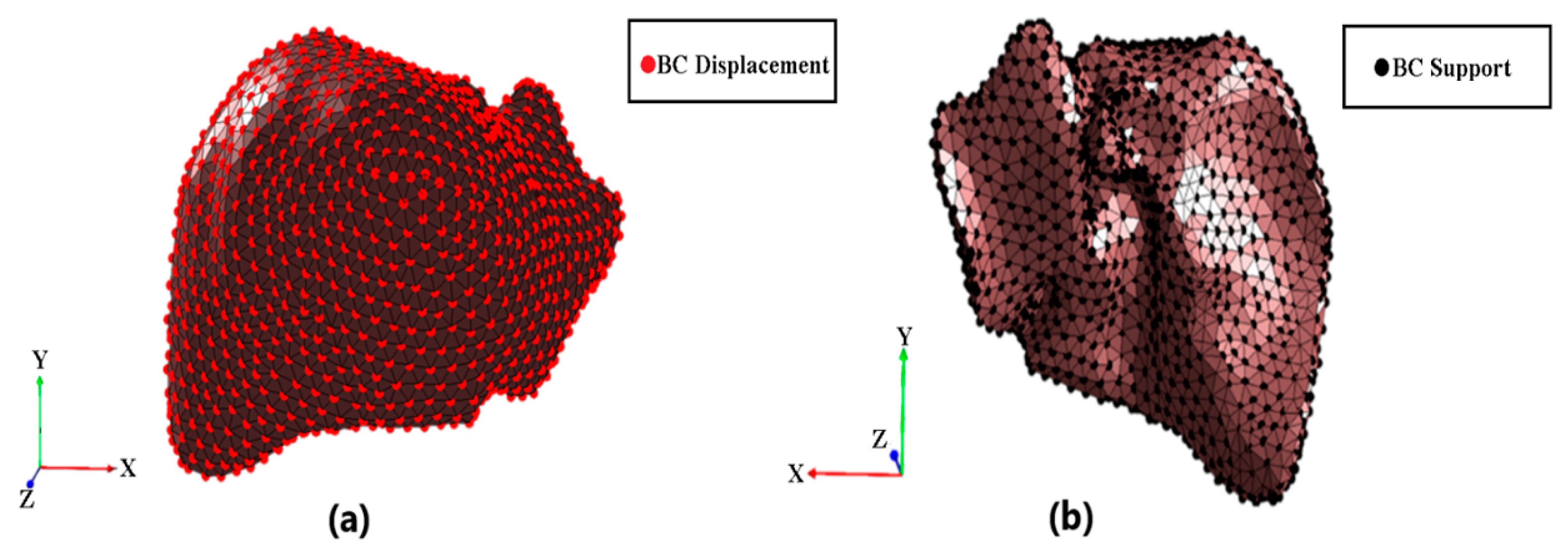
The nodes of the three-dimensional model were selected to define the conditions, classifying the nodes into two groups. The first group was related to the nodes of the visceral surface of the tissue, and these were the homogeneous boundary conditions (support nodes). The second group was related to the nodes of the diaphragmatic surface of the tissue. Therefore, they were the non-homogeneous boundary conditions (displacement nodes).

For the process of selecting the nodes, the preprocessor has two ways of selecting the nodes of the three-dimensional model. The first way is by picking logical surfaces, and the second way is through cartesian coordinates; the coordinates given to the preprocessor will retain only the nodes contained within the given coordinates. The node selection criterion for the diaphragmatic surface consisted of mapping the surface in the Cartesian coordinates based on the data structure of the vertices already within the tetrahedral mesh. Figure 11a visualizes the delimitation of the diaphragmatic surface nodes.

The selection criteria were similar to the previous case regarding the visceral surface. However, the surface was mapped with cartesian coordinates based on the face structure of the STL model of the tissue with the tetrahedral mesh. Once the coordinates contained the area of the visceral surface, the delimitation of nodes of the visceral surface were visualized in Figure 11b.

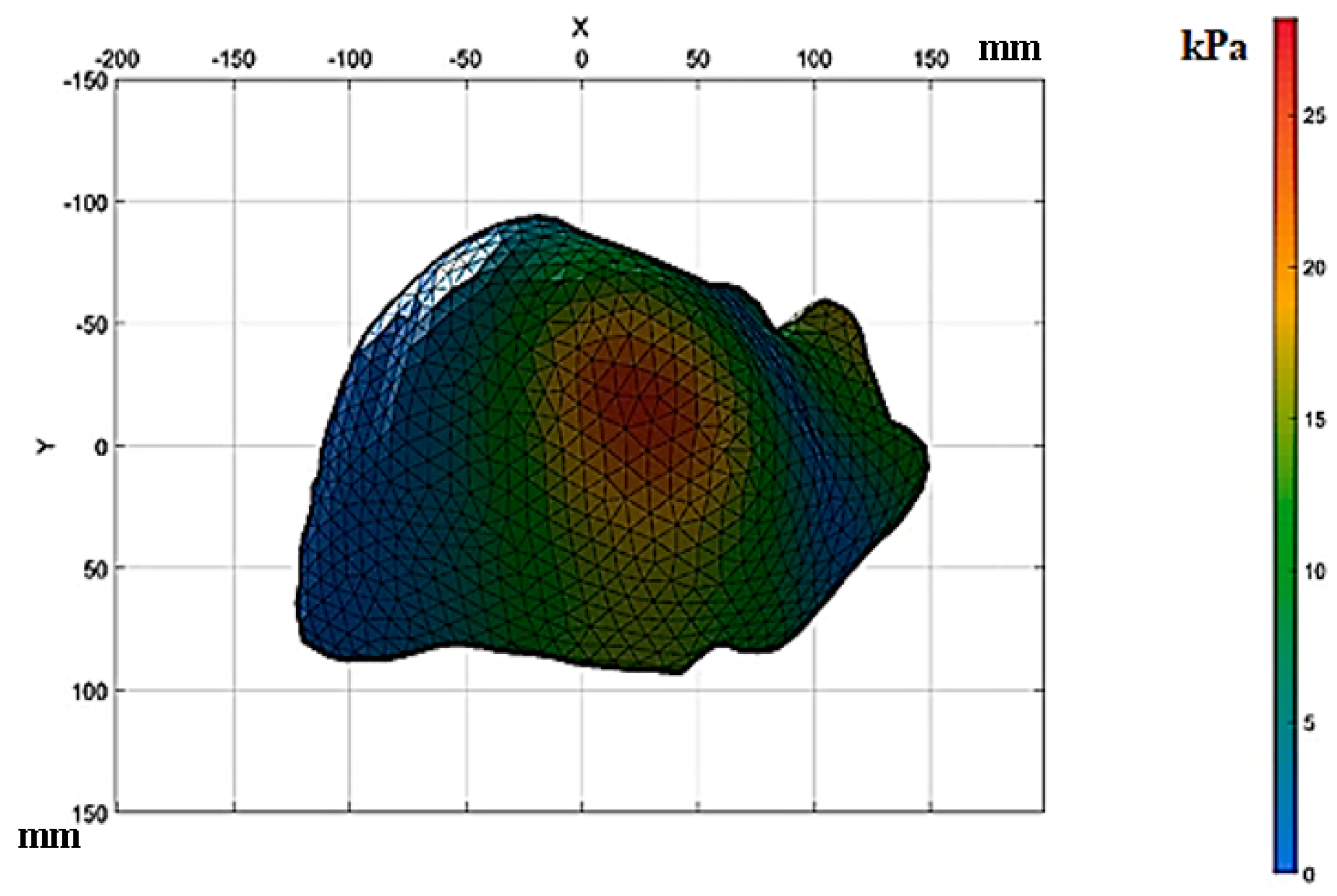
The calculation was made for two study cases; the first one was with properties of healthy tissue, and the second case study used the properties of the tissue with fibrosis with F4-level damage. The results of the numerical analysis of the healthy liver tissue are displayed in Figure 12; the analysis lasted approximately 4 min.

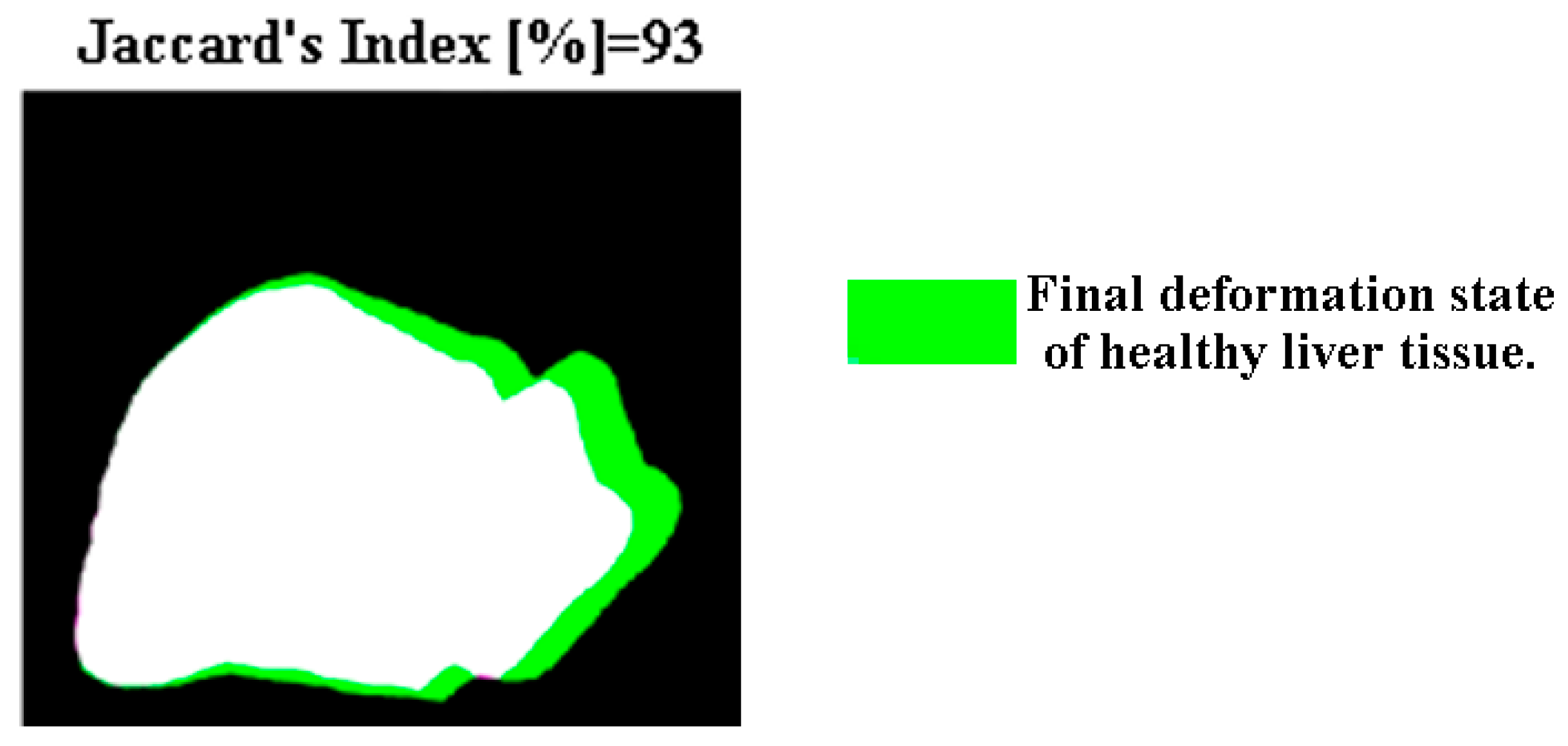
In Figure 12, the stress concentration is addressed in the anterior section of the upper sub-segment. The stresses were approximately 25 kPa and slightly in the upper lateral sub-segment. The stresses in this area were approximately 12 kPa based on the classification of Healey and Schroy [30]. The liver tissue segmentation without deformations and with deformations was performed and converted into binary images.

The view of the diaphragmatic surface corresponding to the X and Y axes provides a visualization of the most tissue surface. Taking the binary images, the code began by calculating the Jaccard similarity between the state without deformation and with deformation. In Figure 13, the results of the Jaccard similarity coefficient are displayed. Based on the results displayed, the healthy liver tissue under a compression load of 12,356 N had a similarity of 93%, which means that it underwent a deformation of 7% on the diaphragmatic surface.

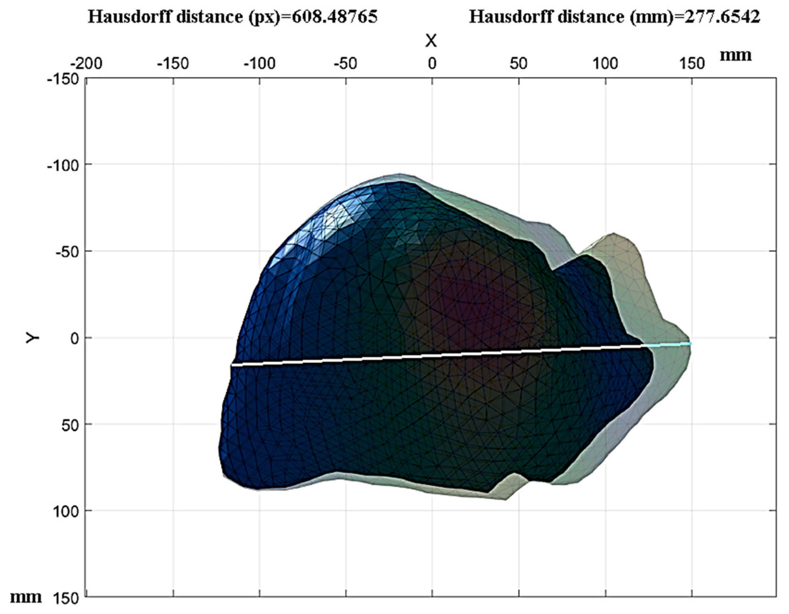
The Hausdorff distance was used to determine the displacements during the compression load. The image sequence of interest was the initial state of the analysis and the final state at the end, emphasizing that the images must be the same size to avoid errors in calculating the measurements. Based on the results displayed in Figure 14, a healthy liver tissue under a compression load of 12,356 N presented in its initial state with a length on the diaphragmatic surface of 242.8 mm, and in the final state, it presented a length of 277.65 mm.

The results were analyzed using the hyperelastic Mooney–Rivlin model with two deformation invariants and an additional invariant that helped to avoid numerical instability. The Mooney–Rivlin model is a reliable and flexible option for analyzing the mechanical behavior of biological tissues due to its ability to describe nonlinear, isotropic, and anisotropic behaviors and its adaptability to consider incompressibility and viscoelastic effects. Linked to the finite element method, its use provides a powerful tool to study and understand the mechanical properties of tissues and their responses to different loading and deformation conditions. It has important applications in medical and biomedical research, biomechanics, and the design of medical devices and treatments. In the literature, several constitutive models are used to analyze the mechanical behavior of biological tissues using this model.

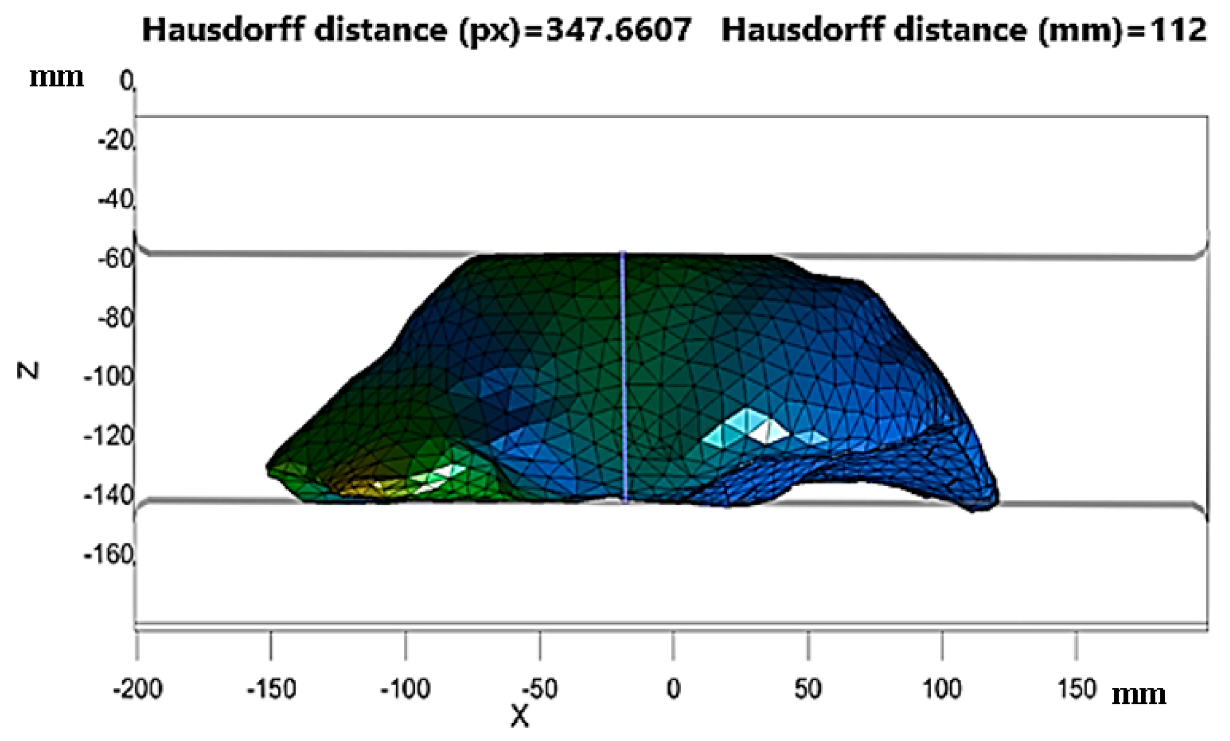
The third reduced invariant for both study cases presented a value of 1, which means that both liver tissues behaved like incompressible material. This means that their volumes were preserved during the deformation. Therefore, this required using a penalty method that avoided numerical instability. This method uses the volumetric modulus to make the calculations converge, and thus, avoids numerical instability. For the calculation of the vertical deformation, the heights in the initial and final states of the analysis carried out previously were considered. 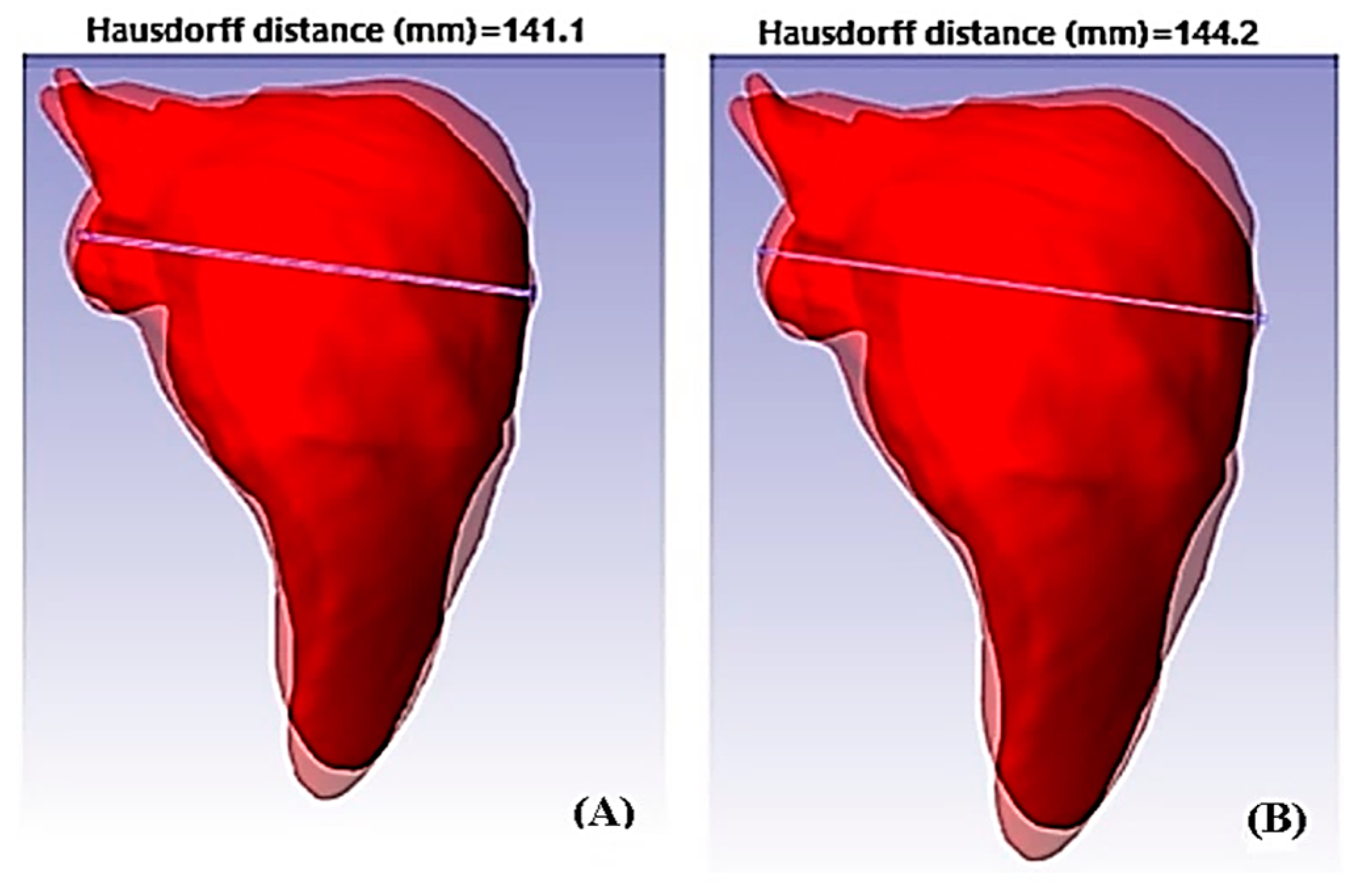The heights are displayed in Figure 15, and the measurements of the heights were made using the Hausdorff distance code.

Figure 15 shows that the final height was 112 mm, while the initial height was 143.6 mm. The initial height was considerably reduced due to the vertical deformation of healthy liver tissue. The results are as follows.

$$I_z\left(z=0\right)=0.77994$$

The deformation invariants for the first case study related to the healthy liver tissue are displayed in

Table 3. Invariants of deformations for healthy liver tissue.

Strain Invariants for Healthy Liver Tissue
I1 = 3.1726
I2 = 3.2038
I3 = 1

.

The reduced invariants for the first case study related to healthy liver tissue are observed in

Table 4. Reduced Invariants for Healthy Liver Tissue.

Reduced Invariants for Healthy Liver Tissue
J1 = 3.1726
J2 = 3.2038
J3 = 1

.

For the first case study corresponding to healthy liver tissue, the constants of the liver tissue are as follows.

$$\begin{gathered} C1=-343.013 Pa \\ C2=343.013 Pa \end{gathered}$$

Finally, the first case study determined the strain energy density function and avoided numerical instabilities. The bulk modulus obtained above was used.

$$W=13.224$$

In the second study case, the properties determined for the affected tissue pathology of fibrosis were considered by the collagen concentration for F4-level fibrosis, with the proportionality between the previously calculated properties and the percentages of collagen in healthy conditions (F0) and with fibrosis (F4).

The approximate properties are displayed in

Table 5. Properties of liver tissue with fibrosis levels F0 and F4.

Fibrosis Level	F4	F0
Young’s modulus	$E=6814.1356 Pa$	$E=2016.9174 Pa$
Modulus of rigidity	$G=2317.7321 Pa$	$G=683.700 Pa$
Volumetric module	$K=37,856.3090 Pa$	$K=13,446.116 Pa$

. The behaviors of the liver tissue affected by fibrosis in the F4-level analysis are shown in Figure 16.

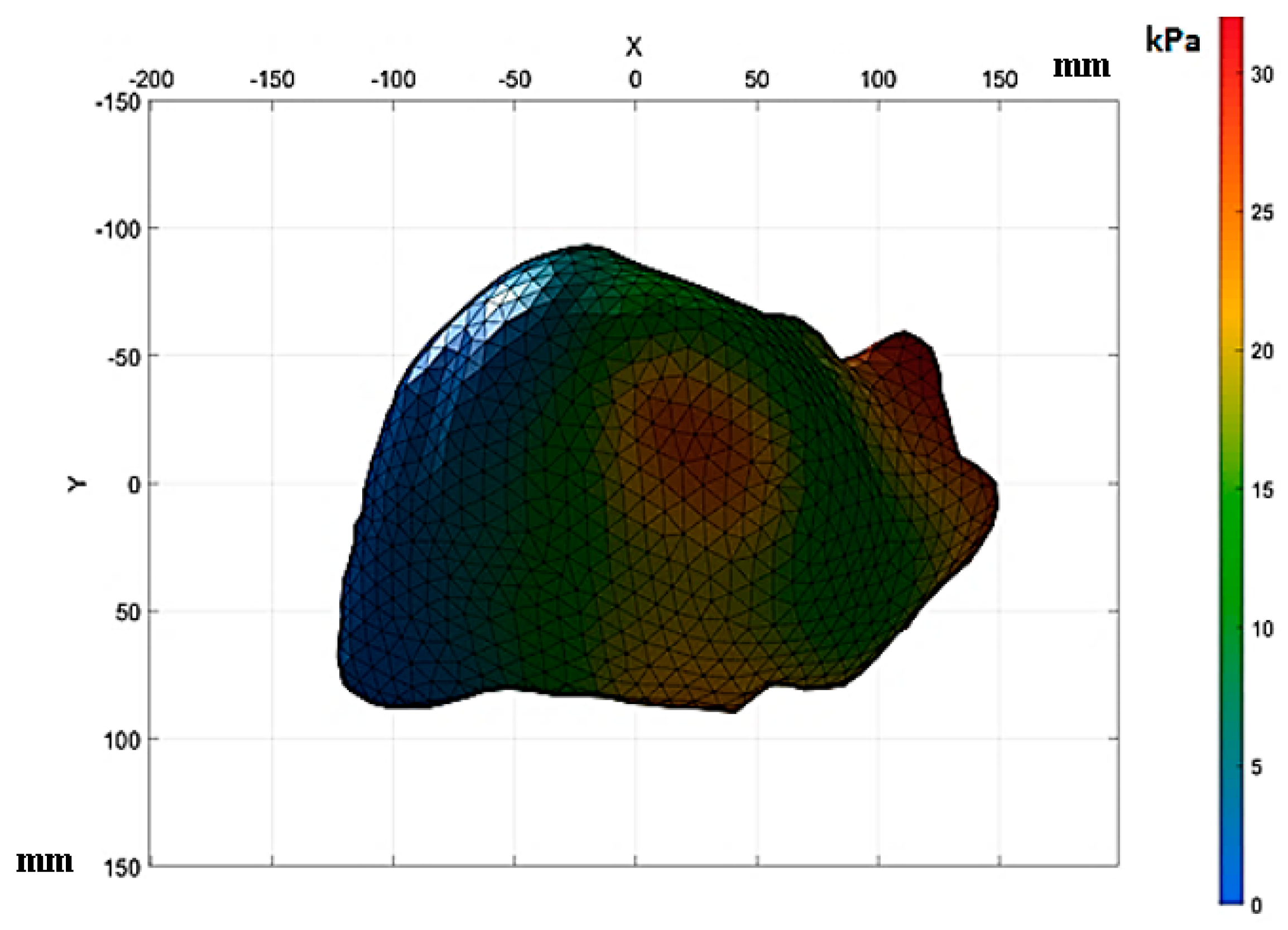
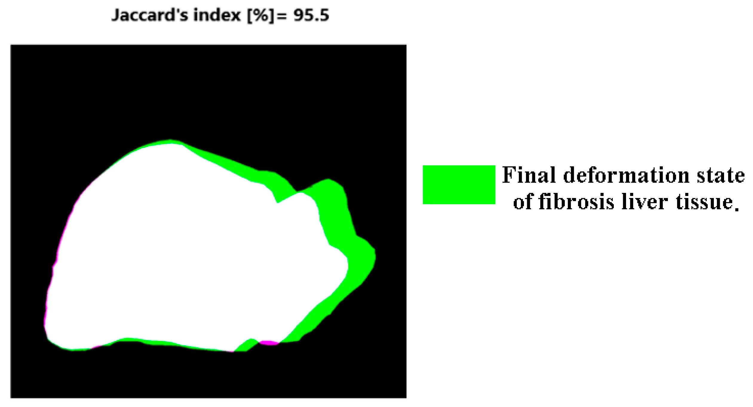
Figure 16 shows the stresses in the anterior section of the upper sub-segment. These stresses were approximately 21 kPa to 30 kPa. In the upper lateral sub-segment, the stresses in this area were approximately 25 kPa to 30 kPa, according to Healey and Schroy [30]. The stress concentrations shown above were due to the increased scar surface caused by fibrosis, causing a decrease in the tissue elasticity. This section analyzes the deformations in the liver tissue affected by advanced fibrosis under a compression load of 12,356 N. It was analyzed using the code used to determine the Jaccard similarity. Based on the binary images, the similarity between states without deformation and with deformation was determined, as displayed in Figure 17. Liver tissue with advanced fibrosis (F4) under a compressive load of 12,356 N presented a similarity of 95.5%. On the other hand, the tissue with fibrosis presented a deformation of 4.5% on the diaphragmatic surface.

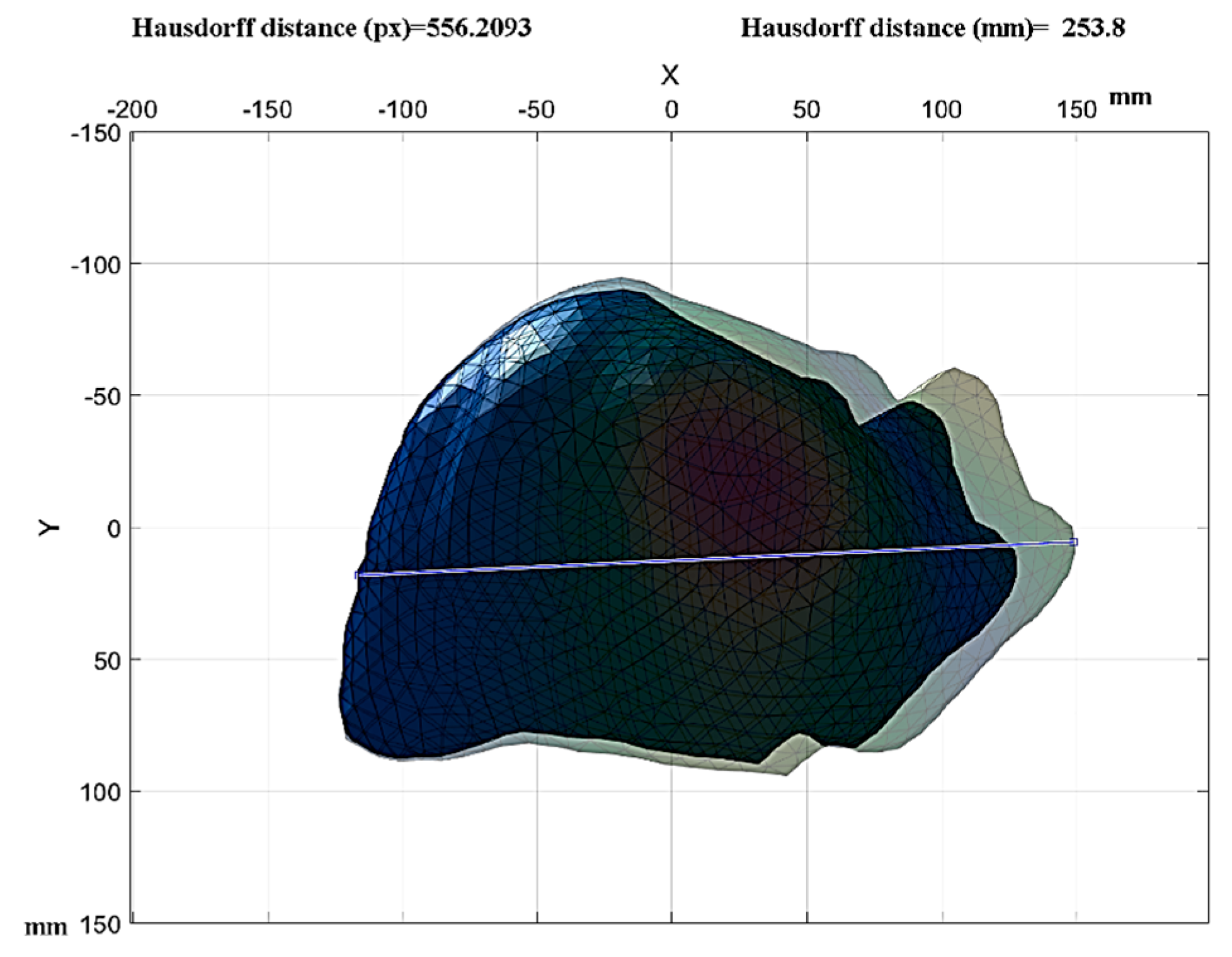
The methodology used for healthy tissue was used for liver tissue with advanced fibrosis, and Figure 18 shows the final stage of the tissue analysis with advanced fibrosis. Its final length was reduced by 4260 mm compared to the healthy tissue, with a total length of 253.8 mm.

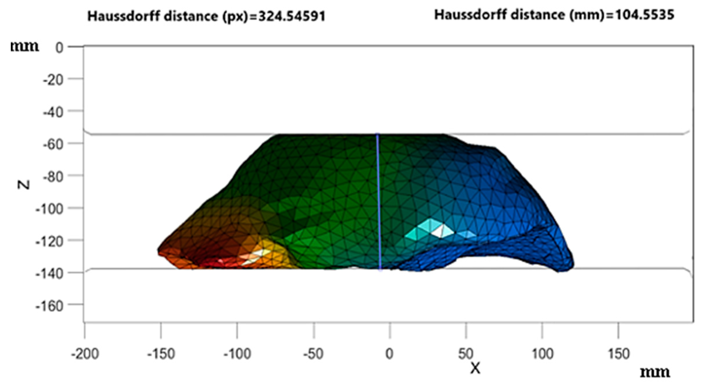
The heights of the initial and final states of the tissue are displayed in Figure 19.

In Figure 19, the final height is 104.5535 mm. It was considerably reduced from the initial height of 143.6. The vertical deformation of the liver tissue affected with advanced fibrosis was determined, and the result obtained was the following:

$$I_z\left(z=0\right)=0.72808$$

The deformation invariants of the second case study related to healthy liver tissue are displayed in

Table 6. Invariants of deformations in the second case study.

Strain Invariants of Liver Tissue Affected by Advanced Fibrosis
I1 = 3.2770
I2 = 3.3426
I3 = 1

.

The reduced invariants of the second case study related to healthy liver tissue are shown in

Table 7. Reduced invariants of the second case study.

Reduced Invariants of Liver Tissue Affected by Advanced Fibrosis
J1 = 3.2770
J2 = 3.3426
J3 = 1

.

Finally, the deformation energy density function was obtained based on Equation 6. The constants C1 and C2 were as follows.

$$\begin{gathered} C1=-1158.86605 \\ C2=1158.86605 \end{gathered}$$

The deformation energy density function was determined for the second case study, which was the following.

$$W=55.49536$$

A code was developed to determine the stresses and deformations that occurred during the analysis using the image sequences resulting from the analysis. There was a sequence of 29 images for the first case study, and the second case study consisted of 30 images. The stress was determined where the Jacobian (J) value was analyzed with the determinant of the deformation gradient, where “F” represents the deformation gradient, and “S” represents the second Piola Kirchhoff stress. The latter was calculated using Equation (3).

$$S=C_1{J}_{1,E}+C_2{J}_{2,E}+K\left(J_3-1\right)J_{3,E}$$

(3)

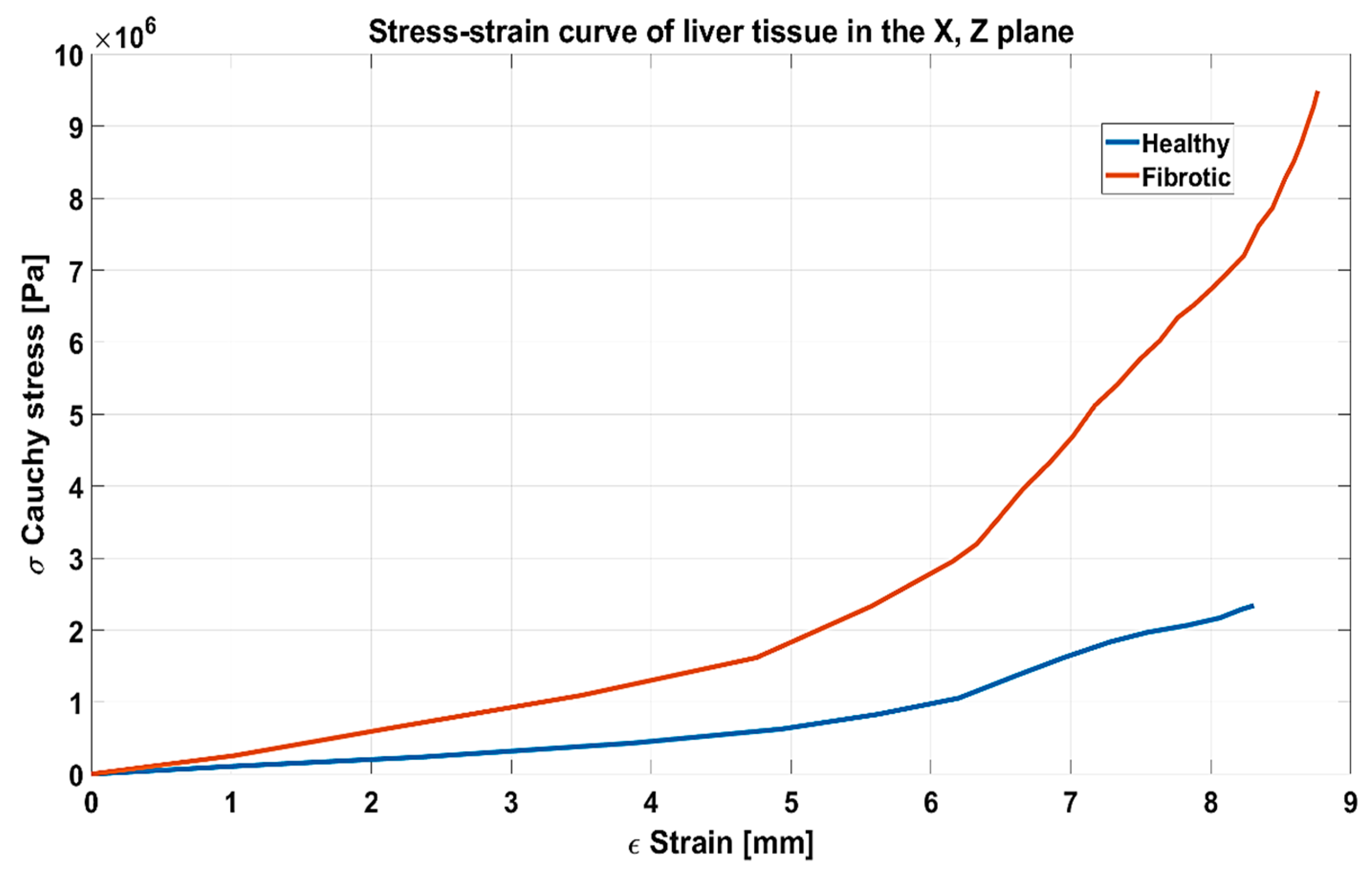
The stress comparison response to the deformations is visualized in Figure 20. It can be observed that the liver tissue affected with fibrosis required more significant compression to be deformed. This means that the fibrotic tissue became rigid, unlike the healthy liver tissue, so it is concluded that the stiffness depends on the saturation of collagen in the liver tissue, which will cause the tissue affected by the fibrosis pathology to become more fragile, which is susceptible to lacerations on its surface.

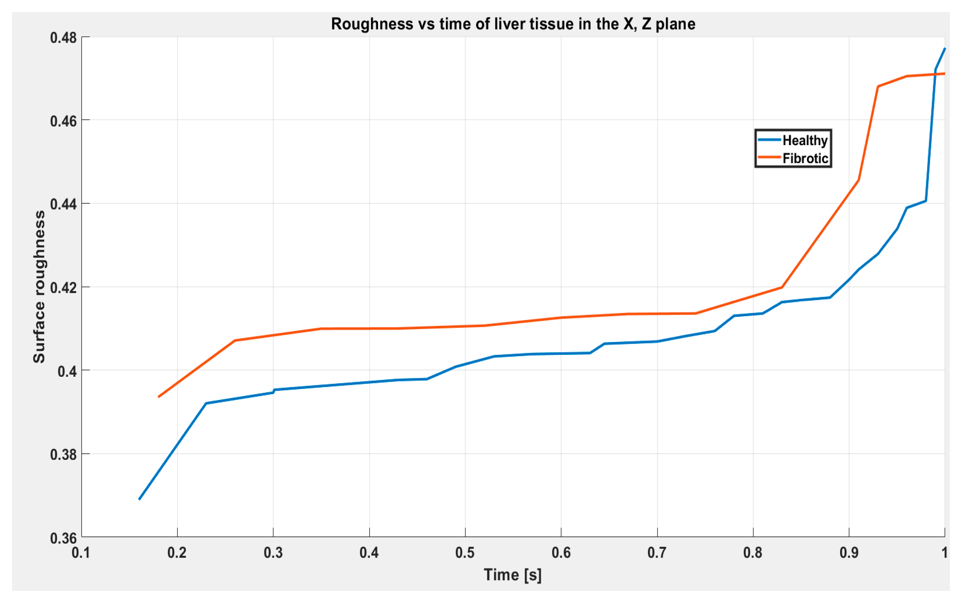
In this work, an analysis of the surface roughness of liver tissue was carried out in healthy conditions and fibrosis conditions affected by fibrosis. The roughness of the liver surface is a crucial characteristic that can provide detailed information on the mechanical properties of the tissue. Using the Hausdorff fractal distance, it was possible to quantify the roughness of the liver surface accurately and objectively at different points during the compression test performed numerically.

The Hausdorff fractal dimension (HFD) was determined using MATLAB^® software. This method was performed by counting 2D boxes. The accuracy of this method depends on several factors, such as the quality of the images in this study, the resolution of 2048 × 1080 pixels used for the analysis, the image processing technique, and the robustness of the algorithm used to calculate the fractal Hausdorff distance. The calculation of the HFD for this study was determined based on Equation (2). To carry out the calculation, the images of the FEM analysis had to be converted into binary images. Later, the program determined the appropriate box size for the determined input image. Above, the program calculated the number of boxes covering the image for each box size. Finishing this calculation, the program fit a straight line to the logarithmic values of the number of boxes based on the logarithm of the box size to determine the fractal dimension from the fitted line.

Measuring liver roughness using the fractal Hausdorff distance provides insight into the complexity and irregularity of the structure of liver tissue affected by fibrosis. A greater roughness may be associated with greater severity of fibrosis and, therefore, with more significant physiological damage.

In particular, for random fractal surfaces, the roughness is related to the fractal dimension by Equation (4):

$$RG=\frac{HFD}{2+c}$$

(4)

RG is the roughness, HFD is the Hausdorff fractal dimension, and C is a constant that depends on the surface type and is generally considered 0.5 for random surfaces. The direct relationship between fractal dimension and roughness is sometimes used without the constant since the constant for specific fractal structures may differ from 0.5.

The fractal dimension is divided by two to obtain the roughness, and the fractal dimension measures the fractal complexity of the image or surface, which considers the amount of detail present at different resolution scales. Roughness, on the other hand, measures the level of detail of the image or surface. For this study, the images obtained from the FEM analysis were chosen as the analysis images, which represent the final height of the final state of deformation in the numerical simulation for healthy liver and liver with fibrosis, as shown in Figure 21.

Figure 21 shows significant differences in the surface roughness between the healthy conditions and those affected by fibrosis. In the healthy liver tissue group, minimal surface roughness and close to ideal fractal structure were observed, indicating a smoother and more homogeneous surface. On the contrary, a notable increase in the surface roughness was observed in the group of liver tissue with fibrosis, showing more significant irregularity and fractal complexity. These outcomes highlight the utility of the Hausdorff fractal distance as a valuable tool in the characterization of roughness and the evaluation of surface changes in biological tissues subjected to mechanical loads. Furthermore, this difference in roughness could be significant for the mechanical analysis of tissue. With greater roughness, there are likely changes in the mechanical properties of the tissue, which could affect its behavior and response to external mechanical loads.

4. Discussion

This work shows a numerical simulation model using a finite element method that simulates human liver tissue’s mechanical response under conditions of damage caused by fibrosis pathology, using MATLAB^® together with a complement biomechanical analysis for this same computer program. The mechanical response of liver tissue affected by fibrosis is related to its structural composition. Therefore, in this research, two case studies were developed. The first was linked to healthy liver tissue, from which Young’s modulus was obtained with other mechanical properties of the tissue based on the respiratory cycle.

In addition, a simulation was performed using the finite element of healthy liver tissue under a compression load on the diaphragmatic surface. The second case study was a numerical simulation of liver tissue affected by advanced fibrosis under a compression load on the diaphragmatic surface. The numerical model evaluated the hyperelastic response of the tissue in healthy conditions and damaged conditions. For this research, two three-dimensional liver tissue models were developed during the respiratory cycle, using medical tomography corresponding to a 38-year-old man.

The results of the proposed numerical simulations were the following: for the healthy tissue, there were stress concentrations in the anterior section of the upper subsegment and in the section of the upper lateral subsegment belonging to the diaphragmatic surface; these stresses were approximately 29 kPa. For the liver tissue affected by fibrosis, the stress concentration was found in the anterior section of the superior subsegment, in the medial inferior subsegment section, and in the anterior inferior subsegment section; these stresses were approximately 34 kPa. To determine the total deformations on the diaphragmatic surface of the tissue, a tool was designed in MATLAB^® that obtained the Jaccard similarity coefficient through images. For the case of healthy tissue, it underwent a deformation of 7% on the diaphragmatic surface, and for tissue affected by fibrosis, it presented a deformation of 4.5% on the diaphragmatic surface. The displacements that occurred during the compression load were determined using the Hausdorff algorithm, which was designed in MATLAB^®. For the case of the healthy tissue in its final state, it had a length of 277.6542 mm, and the tissue affected by fibrosis presented a total length of 253.8 mm. This reduction was due to a superior stiffness on its surface. The hyperelastic response of the liver tissue was determined by the Mooney–Rivlin model. The friction between the contact surfaces was considered with a zero value. It can be assumed that liver tissue expanded uniformly during compression with the above. Table 3 presents that the liver tissue exhibited a linear behavior since the liver tissue suffered a deformation of 6.54% during the inspiration on the upper part of the left and right lobes, respectively. The diaphragm contraction caused this deformation during inspiration; this contraction generated a compression force of approximately 12,356 N. Also, in

Table 8. Properties of liver tissue in its linear part.

Comparison of the Properties of Liver Tissue in Its Linear Part
Property	Healthy Liver Tissue (Obtained)	Healthy Liver Tissue (Literature) [35]	Liver tissue with Fibrosis (Obtained)
Young’s modulus	$E=2016.91 Pa$	$E=2000 Pa$	$E=6814.13 Pa$
Modulus of rigidity	$G=686.7026 Pa$	$G=680.27 Pa$	$G=2317.7321 Pa$
Volumetric module	$K=11,205.096 Pa$	$K=11,110 Pa$	$K=37,856.3090 Pa$
Poisson’s ratio	$v=0.470$	$v=0.47$	$v=0.4750$

, the properties obtained in vitro during the respiratory cycle found by the author Alexandre Hostettler are shown and are similar to those found in this research work [35].

The liver tissue’s properties presenting nonlinear behavior are shown in

Table 9. Properties of liver tissue in its nonlinear part.

Comparison of the Properties Of Liver Tissue In Its Nonlinear Part
Property	Healthy Liver Tissue (Obtained)	Liver Tissue with Fibrosis (Obtained)
The density of strain energy	$W=13.224$	$W=55.3072$
Tangential module	$D=45.508 kPa$	$D=176.963 kPa$

, which were obtained using a numerical simulation, from which two properties were obtained. The first property was the deformation energy density, which quantifies the ability to gather elastic energy per unit volume during the analysis. The second property obtained was the tangential modulus, which allows for obtaining an equivalent of Young’s modulus but applied to materials with nonlinear properties. This property was obtained by using the Mooney–Rivlin hyperelastic model.

The results of the Hausdorff fractal dimension (HFD) analysis were determined to evaluate the classification of the level of damage through the recognition of patterns generated on the tissue surface after having performed the compression analysis based on the results obtained in the graphs shown in Figure 21. It was determined that patterns increased on the surface of the tissue affected by fibrosis. This was due to the increase in superficial rigidity caused by scar tissue derived from fibrosis. In this work, a hybrid approach of fractal analysis was used, and finite element simulations revealed a significant correlation between the fractal structure of the fibrous tissue and its mechanical properties. Furthermore, we observed distinctive fractal distribution patterns at different fibrosis stages, suggesting potential markers for early diagnosis and accurate characterization of disease progression.

5. Conclusions

The study presents several novel findings that contribute to the understanding and characterization of liver tissue behavior in the context of fibrosis. Some of the critical novelties and contributions are as follows:

Integration of Image Processing and Numerical Simulation: This study introduces a novel approach by combining image processing tools with numerical simulation using the GibbonCode plugin for MATLAB^®. This integration facilitated the analysis of displacements and deformations generated during the simulation, providing a comprehensive investigation of the biomechanical behavior of liver tissue affected by fibrosis. Characterization of Collagen Concentration and Tissue Stiffness: The study establishes a positive correlation between collagen concentration and tissue stiffness. It reveals that a higher collagen concentration in fibrotic tissue leads to a considerable increase in tissue stiffness, revealing a loss of elasticity. This insight highlights the importance of collagen as a critical determinant of liver tissue mechanical properties in the context of fibrosis. Hyperelastic Response and Tangential Stiffness: The research presents novel findings regarding the hyperelastic response of liver tissue. By analyzing the elastic energy amassed per unit volume (w), the study demonstrates that fibrotic tissue exhibits significantly higher energy storage than healthy tissue. This increase in energy storage is linked to a rise in tangential stiffness, signifying that advanced fibrosis is associated with a substantial gain in tissue rigidity. Stress-Strain Behavior and Fibrotic Tissue Rigidification: The investigation uncovered novel stress–strain behaviors in liver tissue. Collagen fibers in the tissue’s structural composition led to nonlinear patterns.

The study indicates that as fibrosis progresses, the tissue demonstrates increased nonlinearity, requiring higher stress levels for deformation. This finding suggests that fibrotic tissue becomes more rigid than healthy tissue, providing valuable insights into fibrosis-related mechanical alterations. Application of Hausdorff Fractal Distance for Surface Roughness Analysis: The study introduces the novel use of the Hausdorff fractal distance to analyze surface roughness in liver tissue affected by fibrosis. This quantitative and objective assessment of surface changes provides a new method for understanding the morphological and mechanical alterations associated with liver fibrosis. The potential for improved diagnosis, monitoring, and treatment of liver diseases through non-invasive assessment of surface roughness marks a significant contribution to the field. The study’s conclusions offer novel insights into the biomechanical behavior of liver tissue affected by fibrosis. The integration of image processing, numerical simulation, and the novel application of the Hausdorff fractal distance enriches our understanding of fibrosis-related changes in tissue stiffness and surface roughness. These findings hold promise for advancing liver disease management and expanding the potential application of the methodology to study other organs’ biomechanical behavior in the future.