Article

Forecasting the Active Cases of COVID-19 via a New Stochastic Rayleigh Diffusion Process

by
Ahmed Nafidi
1,
Yassine Chakroune
1,
Ramón Gutiérrez-Sánchez
2 and
Abdessamad Tridane
3,*
1
Laboratory of Systems Modelization and Analysis for Decision Support, Department of Mathematics and Computer Science, National School of Applied Science, Hassan First University of Settat, B.P. 218, 26103 Berrechid, Morocco
2
Department of Statistics and Operational Research, Facultad de Ciencias, Compus Fuente Nueva de University of Granada, 18071 Granada, Spain
3
Department of Mathematical Sciences, College of Science, United Arab Emirates University, Al Ain 15551, United Arab Emirates
*
Author to whom correspondence should be addressed.
Fractal Fract. 2023, 7(9), 660; https://doi.org/10.3390/fractalfract7090660
Submission received: 11 June 2023 / Revised: 27 July 2023 / Accepted: 15 August 2023 / Published: 31 August 2023
(This article belongs to the Special Issue Computational and Stochastic Methods for Epidemic Modeling)

Abstract

:
In this work, we study the possibility of using a new non-homogeneous stochastic diffusion process based on the Rayleigh density function to model the evolution of the active cases of COVID-19 in Morocco. First, the main probabilistic characteristics and analytic expression of the proposed process are obtained. Next, the parameters of the model are estimated by the maximum likelihood methodology. This estimation and the subsequent statistical inference are based on the discrete observation of the variable x ( t ) “number of active cases of COVID-19 in Morocco” by using the data for the period of 28 January to 4 March 2022. Then, we analyze the mean functions by using simulated data for fit and forecast purposes. Finally, we explore the illustration of using this new process to fit and forecast the active cases of COVID-19 data.

1. Introduction

The mathematical modeling of infectious diseases is a way in which to study the spread of diseases and their behavior to predict the future trajectories of an epidemic, as well as to help guide public health planning and disease control. The models developed use stochastic processes to estimate the number of infected cases that could occur in the coming weeks or months. This methodology helps researchers simulate real-world possibilities in a virtual environment. On the other hand, diffusion stochastic processes (SDPs) are good mathematical models that describe probabilistic phenomena in several domains, like environment, biology, economics, medicines and others. Some of the SDPs studied in this sense are found in the works of Bertalanffy [1], Gamma [2], Weibull [3] and Lundqvist-Korf [4], who used SDPs to study growth patterns because of their exponential behavior. In addition, Capocelli and Ricciardi [5] were the first to consider a diffusion process that was associated with the Gompertz curve, and this has been applied to several fields of study, such as population growth or neural activity modeling [6]. The logistic diffusion process has been applied to a diverse range of scientific areas; specifically, Capocelli and Ricciardi [7] derived a new diffusion process from a re-parameterization of the logistic model. Giovanis and Skaidas [8] proposed a stochastic logistic model that was analytically solved by using the theoretical framework of reducible stochastic differential equations (SDEs), and these were then applied to study the consumption of electricity in Greece and the United States.
The new virus of SARS-CoV-2, named COVID-19 (Coronavirus 2019) by the World Health Organization (WHO), is believed to have originated from an animal source in the city of Wuhan, Hubei region, China, in December 2019. Since its first appearance, the disease has spread worldwide. On 11 March 2020, the WHO officially classified the epidemic as a pandemic. As of 22 March 2022, the virus (including its variants) has infected 492 million people, with 6.5 million deaths. Several research studies have been developed in the context of modeling the pandemic. For example, see Ref. [9] for the stochastic COVID-19 Levy jump model with an isolation strategy; Ref. [10] introduced a new model for the spread of COVID-19 and the improvement of safety; Ref. [11] constructed a new random infectious disease system under the environmental noise of the infection rate, as well as studied the probability density function (PDF) of the stochastic system; and Ref. [12] applied a mathematical model to describe the behavior of the number of cases with respect to time in Italy.
The Rayleigh distribution was developed by the physicist Lord Rayleigh [13], and it is widely used in physics-related fields to model processes such as sound and light radiation, wind speed, and wave height. It is also used in communications theory to describe the hourly median and instantaneous peak power of received radio signals (see, [14]). In addition, it plays a crucial role in the field of land mobile radio as it can accurately describe wind speed. Thus, the Rayleigh distribution has a wide use in many fields, which makes its study from dynamic and stochastic point of views interesting (see for example, [15]).
The problem of statistical inference in SDPs has attracted a great deal of interest in recent years, and this applies both when the process is considered continuously or discretely. In general, the estimation of parameters in stochastic models is not direct apart from in simple cases, and one possible method is based on the approximation of the maximum likelihood (ML) function. In this context, various methods have been developed to address this problem. The basic case for this approach can be found in Bibby and Sorensen [16], as well as in Ait-Sahalia [17]. The method of estimating the ML of the parameters when using likelihood equations can be difficult to implement, which is the reason why we propose to use the simulated annealing (SA) method for estimating the parameters in an SDP (see, for instance, [3,4]).
In this work, based on previous research in this field, we introduce a stochastic Rayleigh diffusion process (SRDP) whose mean is proportional to the Rayleigh density function (RDF). The SRDP is used to model the evolution of the active cases of COVID-19, and this is the first attempt to use the stochastic Rayleigh diffusion process to model a pandemic. The SRDP was introduced by [18] to model female and male life expectancy at birth in Spain. A brief version of this process was introduced by [19], and we specifically call this method the Ornstein–Uhlenbeck radial process. This process has also been studied and applied by [20] to model the production of thermal energy in the Maghreb. The Rayleigh process has also been used to model the exchange rate dynamics when using the Swiss Franc against the Euro under a floating-rate regime [21], as well as for the statistical inference and computational aspects of the stochastic Rayleigh diffusion model [22].
In the present paper, we introduce a new SRDP that is different from the one studied in [22]. This SRDP is based on RDF, and the paper is organized in the following way: In Section 2, we describe how the explicit form of this SRDP model is given by Itô’s lemma. Moreover, we give all the main characteristics of the proposed process, such as the transition PDF (TPDF), mean function (MF) and the conditional mean function (CMF). In Section 3, we adopt the ML to find the estimators of the parameters of our model. The parameter estimators are found by solving the ML equations. That said, in this case, we cannot find the solution directly, so we use the numerical method of simulated annealing (SA). In Section 4, we simulate the SRDP through using its explicit form. We also observe the behavior of the SRDP trajectories for the different values of parameters of the diffusion coefficient. We then use the simulated data to obtain the estimators of our given parameters by applying the adopted numerical method. Furthermore, we predict some of the realizations by using the estimated MF (EMF) and conditional CMF (ECMF). Section 5, offers an application of this process through an exploration of the development of the active COVID-19 cases in Morocco from January to February 2022. In the last section, we detail the conclusion of our findings.

2. The Proposed SRDP

In this section, we introduce the new SRDP, whose mean function is proportional to the Rayleigh one. We also determine how the SDE solution can be explicitly expressed with its probabilistic characteristics.

2.1. Definition of the SDE of the SRDP

The RDF is defined by
x ( t ) = t α 2 exp t 2 2 α 2 ; t > 0 .
By differentiation of Equation (1) with respect to t, we obtain the following:
d x ( t ) d t = t α 2 exp t 2 2 α 2 1 t t α 2 .
When considering g ( t ) = 1 t t α 2 , Equation (2) becomes
d x ( t ) d t = g ( t ) x ( t ) ; t > 0 .
When we replace g ( t ) by g ( t ) + σ w ( t ) , we obtain the following SDE:
d x ( t ) = g ( t ) x ( t ) d t + σ x ( t ) d w ( t ) ; x ( t 1 ) = x 1 ,
with w ( t ) as a Brownian motion, x 1 is a positive random variable, which is independent of x ( t ) for t t 1 and t 1 > 0 . By applying Itô’s formula, we obtain the expression of the process x ( t ) : t t 1 , with infinitesimal moments:
B 1 ( x , t ) = g ( t ) x ( t ) ; B 2 ( x , t ) = σ 2 x 2 ( t ) .
The functions B 1 ( x , t ) and B 2 ( x , t ) in Equation (5) are measurable in the sense of Borel, and they meet the uniform Lipschitz and the growth conditions (see [18]). Afterward, our SDE ( 4 ) has a unique solution { x ( t ) : t [ t 1 ; T ] } , which is continuous with probability 1 and meets the initial condition P ( x ( t 1 ) = x 1 ) = 1 .

2.2. The Explicit Form of the SRDP

We address the transformation form z ( t ) = ln ( x ( t ) ) , and apply it to Itô’s formula. Thus, the obtained SDE ( 4 ) is as follows:
d z ( t ) = g ( t ) σ 2 2 d t + σ d w ( t ) = 1 t t α 2 σ 2 2 d t + σ d w ( t ) .
By integrating the two sides, we obtain
z ( t ) = z ( t 1 ) + ln t t 1 1 2 α 2 ( t 2 t 1 2 ) 1 2 σ 2 ( t t 1 ) + σ ( w ( t ) w ( t 1 ) ) .
Thus, from the latter and due to the result in [23], a necessary and sufficient condition for z ( t ) to be a Gaussian process is that ln ( x 1 ) must be normally distributed or constant.
When the initial condition x ( t 1 ) = x 1 is taken into account, then the solution of the SDE ( 4 ) from the ( 7 ) can be explicitly expressed as follows:
x ( t ) = x t 1 t t 1 exp 1 2 α 2 ( t 2 t 1 2 ) 1 2 σ 2 ( t t 1 ) + σ ( w ( t ) w ( t 1 ) ) .

2.3. Characteristics of the SRDP

2.3.1. The TPDF of the Process

Regarding the SRDP expression in Equation (8), we find
x ( t ) Λ 1 ( μ ( t , s , x s ) , σ 2 ( t s ) ) .
We can then determine the TDPF of the SRDP for t > s as
f ( x , t x s ; s ) = 1 σ x s 2 π ( t s ) exp ln ( x ) μ ( t , s , x s ) 2 2 σ 2 ( t s ) ,
with μ ( t , s , x s ) = ln x s + ln t s 1 2 α 2 ( t 2 s 2 ) σ 2 2 ( t s ) .

2.3.2. The r-th Conditional and Its Mean Functions

Based on the fact that { x ( t ) x ( s ) = x s } is a lognormal process, the rth conditional moments of the SRDP are as follows:
E ( x r x ( s ) = x s ) = exp r μ ( s , t , x s ) + r 2 σ 2 2 ( t s ) = x s t s r exp r 1 2 α 2 ( t 2 s 2 ) σ 2 2 ( t s ) + r 2 σ 2 ( t s ) .
When r = 1 , then the CMF is
E x ( t ) x ( s ) = x s = x s t s exp 1 2 α 2 ( t 2 s 2 ) .
By taking into account the degenerate distribution P ( x ( t 1 ) = x 1 ) = 1 , the MF is
m ( t ) = x 1 t t 1 exp t 1 2 2 α 2 exp t 2 2 α 2 .

2.4. Remark

In the case where σ = 0 i.e., in the absence of white noise, Equation ( 4 ) has a unique solution of x ( t ) = k t exp t 2 2 α 2 , which is proportional to the Rayleigh curve f ( t ; α ) = k t exp t 2 2 α 2 with α > 1 .

3. Inference on the SRDP

3.1. The Model Estimation by Using the ML

The SRDP parameters can be estimated via a discrete sampling that drives from the likelihood function, and this originates in the transitions of the process. Let us take the discrete sample x ( t i ) = x i , of the process i = 1 , , n during t 1 , , t n . We thus take t i t i 1 = h for i = 2 , , n . The parameters estimated through the ML include θ = ( β , σ 2 ) , where β = 1 α 2 . The likelihood function is then given by
L ( x 1 , , x n ; θ ) = i = 2 n f θ ( x i , t i x i 1 ; t i 1 ) ,
When we search for the value of θ maximizing L, to this end, we search for a solution to this differential system:
θ j i = 2 n f θ ( x i , t i x i 1 ; t i 1 ) ; j = 1 , 2 .
The logarithm of L is
ln L ( x 1 , , x n ) β ; σ 2 = ln i = 2 n f θ x i , t i x i 1 ; t i 1 .
Then,
ln L ( x 1 , , x n ) = 1 2 σ 2 i = 2 n 1 t i t i 1 ln x i x i 1 ln t i t i 1 + β 2 t i 2 t i 1 2 + σ 2 2 t i t i 1 2 i = 2 n ln σ x i 2 π ( t i t t 1 ) .
We thus consider h = t i t i 1 and θ i , β = ln x i x i 1 ln t i t i 1 + β 2 t i 2 t i 1 2 , and we obtain
ln L ( x 1 , , x n ) = ( n 1 ) 2 ln σ 2 + ln ( 2 π h ) i = 2 n ln x i 1 2 σ 2 h i = 2 n θ i , β + σ 2 2 h 2 .
Regarding the derivative of ln L with respect to β and σ 2 , we obtain
ln L β = 1 2 σ 2 i = 2 n ( t i + t i 1 ) θ i , β + σ 2 2 h
ln L σ 2 = ( n 1 ) 2 σ 2 1 2 σ 4 h i = 2 n θ i , β + σ 2 2 h 2 + 1 2 σ 2 i = 2 n θ i , β + σ 2 2 h .
By setting the last Equations (15) and (16) as being equal to zero, we find the following:
i = 2 n ( t i + t i 1 ) θ i , β + σ 2 2 h = 0 . ( n 1 ) σ 2 + 1 h i = 2 n θ i , β + σ 2 2 h 2 σ 2 i = 2 n θ i , β + σ 2 2 h = 0 ,
after a development of the second equation, we obtain
i = 2 n ( t i + t i 1 ) θ i , β + σ 2 2 h = 0 . ( 1 ) h 2 4 σ 4 + h σ 2 1 n 1 i = 2 n θ i , β 2 = 0 . ( 2 )
The second equation of the set equations is a quadratic equation on σ 2 ; thus, we can find the positive solution because the discriminant Δ = h 2 + h 2 ( n 1 ) i = 2 n θ i , β 2 is strictly positive. The ML estimated value of σ 2 is as follows:
σ ^ 2 = 2 h 1 + 1 ( n 1 ) i = 1 n θ ^ i , β 2 1 / 2 1 ,
with
θ ^ i , β = ln x i x i 1 ln t i t i 1 + 1 2 β ^ h t i + t i 1 ,
we then obtain the non-linear equation by substituting the last expression into the second likelihood equation
i = 2 n ( t i + t i 1 ) θ i , β + 1 + 1 ( n 1 ) i = 1 n θ ^ i , β 2 1 / 2 1 = 0 .
To find the second parameter’s estimator, we need to resolve the non linear Equation (18), which could prove to be difficult. Therefore, we opted for the numerical method SA.

3.2. The Model Characteristics Estimation

3.2.1. The MF and CMF Estimation

By considering the Zehna theorem (see [24]), the estimators of the MF and the CMF are given by replacing the values of the parameters in Equations ( 11 ) and ( 12 ) with their estimators. The ECMF can be described as follows:
E ^ ( x x ( s ) = x s ) = x s t s exp 1 2 β ^ t 2 s 2 .
Taking into account the condition P ( x ( t 1 ) = x 1 ) = 1 , the EMF is shown as follows:
E ^ ( x ( t ) ) = x 1 t t 1 × exp 1 2 β ^ t 1 2 × exp 1 2 β ^ t 2 .

3.2.2. Confidence Interval

The confidence interval (CI) of the SRDP was adapted from the procedure that was developed in [25]. Consider u ( s , t ) = x ( t ) x ( s ) = x s and w ( t ) w ( s ) N ( 0 ; ( t s ) ) for t s , so
v = ln ( u ( s , t ) ) μ ( s , t , x s ) σ t s N ( 0 , 1 ) ,
with μ ( s , t , x s ) = ln ( x s ) + ln t s 1 2 β t 2 s 2 σ 2 2 ( t s ) . The conditional CI (CCI) for v a δ % is given by P ( λ v λ ) = δ % .
Then, we can obtain the CI for the variable u ( s , t ) by applying the formula u l o w e r ( s , t ) ; u u p p e r ( s , t ) with
u l o w e r ( s , t ) = exp μ ( s , t , x s ) λ σ t s ,
u u p p e r ( s , t ) = exp μ ( s , t , x s ) + λ σ t s ,
and with λ = F N ( 0 ; 1 ) 1 1 δ 2 , where F N ( 0 ; 1 ) 1 is the inverse cumulative normal standard distribution.
On the other hand, the estimation of the CIs u ^ l o w e r and u ^ u p p e r can be expressed by replacing the parameters by their estimators in Equations (21) and (22). Therefore, the limits of the CIs are
u ^ l o w e r ( s , t ) = exp μ ^ ( s , t , x s ) λ σ ^ t s .
u ^ u p p e r ( s , t ) = exp μ ^ ( s , t , x s ) + λ σ ^ t s ,
with μ ^ ( s , t , x s ) = ln ( x s ) + ln t s 1 2 β ^ t 2 s 2 σ ^ 2 2 ( t s ) .

3.3. Optimization via the SA Algorithm

The SA algorithm is a method designed to optimize the solution of optimization problems. This was introduced by [26]. Through this algorithm, in each iteration, θ is a current solution, and θ is a new value chosen near θ in the following iteration. The objective difference is Δ = g ( θ ) g ( θ ) . If Δ 0 , then θ is chosen as the novel solution. Or else, it may be accepted with a probability p = exp Δ T .

3.3.1. The Objective Function

For the second estimator of the parameter β , we applying a numerical method based on the simulated annealing by looking for the solution of the following unconstrained optimization problem:
min β , σ g ( β , σ 2 ) = ( n 1 ) 2 ln σ 2 + 1 2 h σ 2 i = 2 n ln x i x i 1 ln t i t i 1 + β 2 ( t i 2 t i 1 2 ) + σ 2 2 h 2 .

3.3.2. Bounding the Search Space

The solution of Equation (20) is found in the estimators of the parameters β and σ 2 . The solution space is the space where the estimators take their values. It is defined by ] 0 ; + [ × ] 0 ; + [ , and is continuous and unbounded. Then, in some cases, the information provided by the data of the sample, as well as by some characteristics of the model allow one to limit this parameter space (see for, example, [1,27]).
In this section, we numerically construct the boundary spaces for the parameters with process simulations. As for σ , we can see that, if it takes on large values, it leads to sampling paths with a high variability around the mean. As a result, an excessive variability in the available paths would mean that a Rayleigh model is not recommended (see Figure 1). The simulations carried out for different values led us to observe that 0 σ 0.1, which makes it possible to obtain trajectories that are compatible with a Rayleigh-type growth. For the β parameter, a numerical study of the ML function was carried out by varying its values. Through using simulated examples, we derived the ML function, which is defined as β ( 0 , 1 ] . When the solution space is bounded, the initial parameters of the algorithm and the stopping criterion are specified as follows:
1.
Choose the first solution arbitrarily in the obtained bounded subspace.
2.
The initial temperature ( T 0 ) must be sufficiently high for a good probability in accepting a less good solution to be at least 80% (see [26]).
3.
The cooling process is T i = λ T i 1 with λ < 1 being constant. Typically, 0.75 λ 0.95 .
4.
The number of solutions generated at a temperature T is determined by the length L of the chain.
5.
The stopping conditions are indicated when the system reaches the required energy level (freezing temperature), or when an acceptance ratio is reached. In this case, the total number of generated solutions is given. As for the maximal number of iteration, it is fixed to 1000.

4. Numerical Simulation of the SRDP

4.1. Simulation of Sample Path of the SRDP

After having described and studied the main characteristics of the new proposed Rayleigh process in previous sections, we proceed now to introduce some simulations of the process sample path in order to visualize its behaviour and to validate the final proposed model of the new process. We will focus on the form of the SRDP given explicitly by Equation (8). The simulations are based on the generation of 25 sample paths in [ t 1 ; T ] , such that t i = t 1 + ( i 1 ) h with h = T t 1 N for i = 1 , , N (where N is a sample size), as well as x 1 N ( 1 ; 0.5 ) , t 1 = 0.1 , T = 10 and N = 250 . Figure 1 presents the simulated SRDP trajectories for some of the values of σ and α .

4.2. Parameter Estimation of the SRDP

In this section, we suggest several examples that validate our estimation procedure. Thus, we simulate Equation (8) 20 times with the following values: t 1 = 0.1 , h = T t 1 N , x 0 Λ 1 ( 1 ; 0.5 ) and N (which is chosen to be equal to 100 , 200 and 500). This is performed in order to check the impact of the sample size on the results of the estimation methodology.
To perform the inference, we chose for each example, 25 sampled trajectories, such that t i = t 1 + ( i 1 ) h for i = 2 , , N . The obtained results are represented in Table 1, which groups together the empirical mean (EM), the standard deviation (std) and the coefficient of variation (CV) that was obtained for β and σ .
Table 2 illustrates the obtained results from the calculation of those measurements, showing how the methodology works.

4.3. Prediction Study Using EMF and ECMF

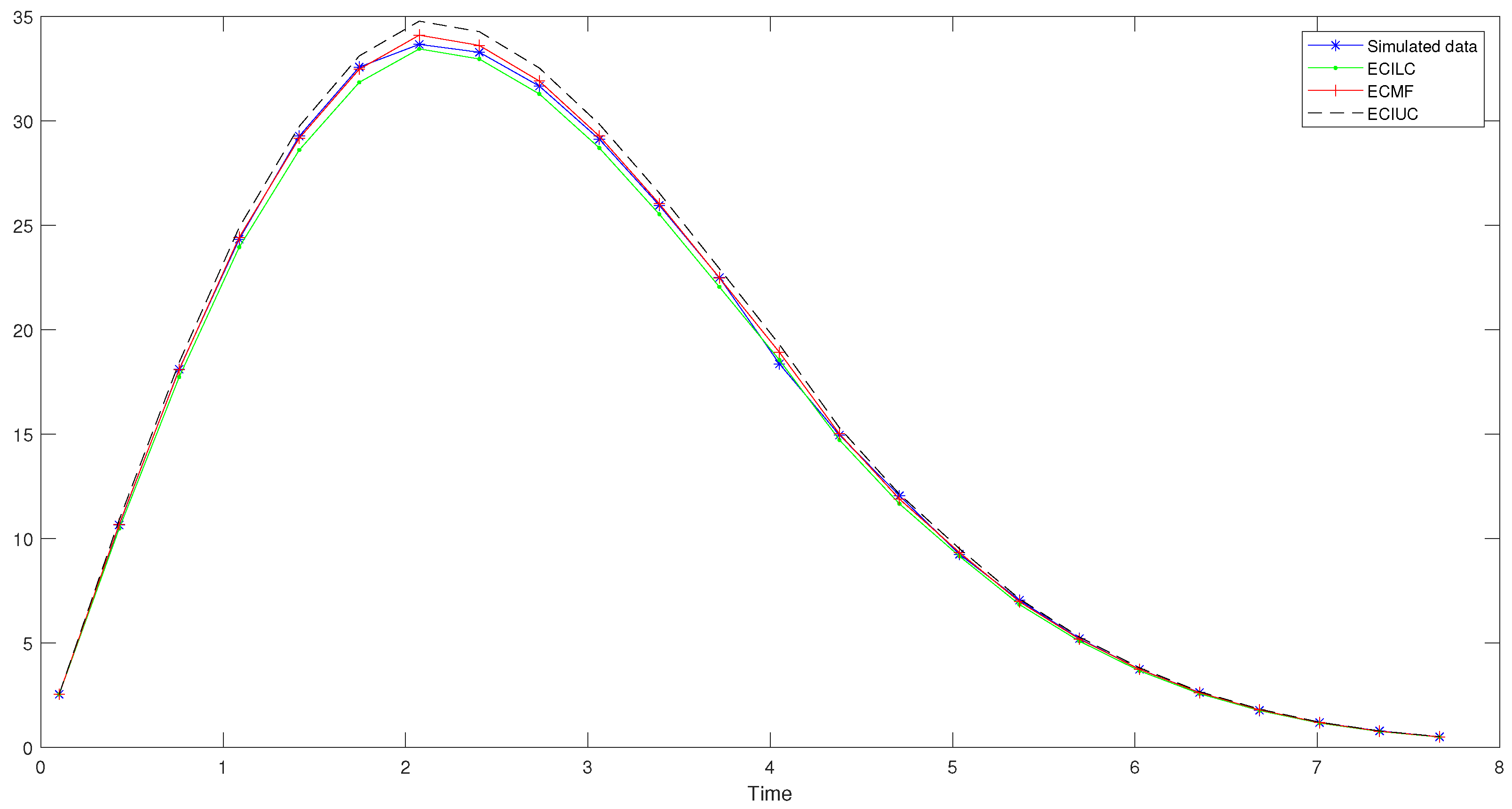
In this section, we consider an application that was established on the simulated SRDP with N = 25, t i = t 1 + ( i 1 ) h and i = 2 , , N . We start with t 1 = 0.1 , as well as with a discretization step of h = T N t 1 N , x 0 = 20 and T N = 10 . We used the first 21 pieces of data to estimate the SRDP parameters β and σ by the SA algorithm. Furthermore, we obtain the values of EMF and ECMF expressed by (11) and (12). We predict the last three values using the Equations (11) and (12). Next, we show the results related to a 95 % (ECI) boundary (ECIB) of the processes (see Equations (23) and (24)). To highlight the methodology developed above, the results were checked using the mean absolute error (MAE), the root mean square error (RMSE) and the mean absolute percentage error (MAPE) (see Table 3).
The MAPE result (see Table 4 and Table 5 ) can be used to judge the performance of the forecast, which was less than 10%, thus showing that the forecast was performing well. The estimated parameters of the SRDP from the simulated data are summarized in Table 6. Table 7 illustrates the results of the simulated data and the estimated values of the EMF, ECMF and ECI of the SRDP process. Figure 2 and Figure 3 show the performance of the SRDP for prediction when using the EMF and ECMF functions.

5. Application to Real Data

The SRDP with the statistical method proposed above was used to study the evolution of the active cases of COVID-19 when considering the EMF and the ECMF. The process x ( t ) represents the number of COVID-19 active cases, and we have taken the period of 4 January to 27 February 2022 to fit the model.
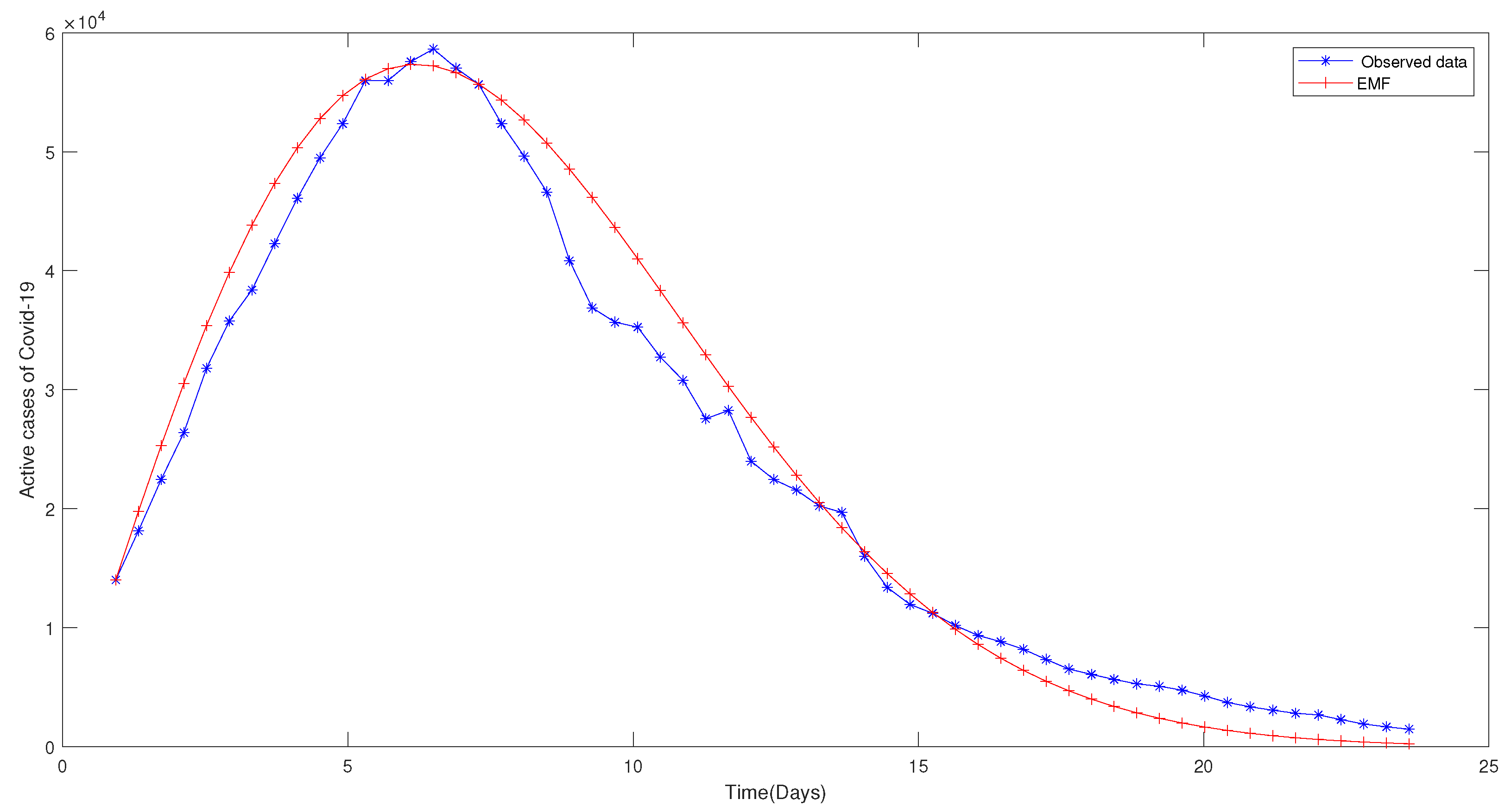
Let us take t i = t 1 + ( i 1 ) h for i = 2 , , N with t 1 = 0.1 , where the step size is h = T N t 1 N , and where T N = 26 , N = 37 and x 1 = 13450 . We used the series of observations considered between 28 January and 4 March 2022 of the COVID-19 active cases to estimate the parameters of the SRDP through using the SA algorithm, thus we found β ^ = 0.393749 and σ ^ = 0.04 . By using the MF and CMF, we predicted the corresponding results for the days of 5 to 9 March by the EMF and ECMF. In addition, we showed the results that were attached to a 95 % ECCI of the SRDP. Table 8 gives the results for the real data, the EMF, the ECMF and the ECCI. Figure 4 and Figure 5 illustrate the real data, the EMF and the ECMF values. This figure shows that the conditional versions are preferable for a better fit to the observed data and for short-term predictions.

6. Conclusions

The recent COVID-19 pandemic had revealed the importance of utilizing different mathematical modeling tools that can help to understand the progress of the disease and can forecast the possible outcome of the pandemic progress. In this work, a diffusion process related to the Rayleigh density function SRDP was introduced to model the progress of the number of COVID-19 active cases. The main characteristics of the proposed model were discussed and analyzed in order to obtain a forecast of the possible cases. The parameters of the SRDP were estimated by applying the ML method and the SA algorithm. Then, based on the simulation of the SRDP, we managed to handle the forecasting phase by using the estimation of the EMF and ECMF, as shown in Table 7. Finally, we proposed an application to study the active cases of COVID-19 in Morocco by adjusting the proposed process to the real data for the period of 4 January to 10 February 2022. We also obtained a good representation of the series and good short-term forecasts (4–10 February). Our model is the first attempt ever to use the stochastic Rayleigh diffusion process in modeling a pandemic. Our next step is to generalize our approach to model the different waves of the pandemic via the superposition stochastic Rayleigh diffusion process.

Author Contributions

Conceptualization, A.N. and Y.C.; Methodology, R.G.-S. and A.T.; Software, Y.C.; Validation, R.G.-S. and A.T.; Formal analysis, A.N. and Y.C.; Investigation, A.N. and Y.C.; Resources, R.G.-S.; Data curation, Y.C.; Writing—original draft, A.N. and Y.C.; Writing—review & editing, A.T.; Visualization, Y.C. and R.G.-S.; Supervision, R.G.-S. and A.T.; Project administration, A.T.; Funding acquisition, A.T. All authors have read and agreed to the published version of the manuscript.

Funding

A. Tridane was supported by the UAEU UPAR, grant number 12S125.

Data Availability Statement

No data availability statement applies.

Acknowledgments

The authors would like thank the anonymous reviewers for their careful preparation of our paper and for their valuable comments that aided us in improving the quality of this work.

Conflicts of Interest

The authors declare that they have no conflict of interest.

References

  1. Román-Román, P.; Torres-Ruiz, F. A stochastic model related to the Richards-type growth curve. Estimation by means of simulated annealing and variable neighborhood search. Appl. Math. Comput. 2015, 266, 579–598. [Google Scholar] [CrossRef]
  2. Gutiérrez, R.; Gutiérrez-Sánchez, R.; Nafidi, A. The trend of the total stock of the private car-petrol in Spain: Stochastic modelling using a new gamma diffusion process. Appl. Energy 2009, 86, 18–24. [Google Scholar] [CrossRef]
  3. Nafidi, A.; Bahij, M.; Achchab, B.; Gutiérrez-Sànchez, R. The stochastic Weibull diffusion process: Computational aspects and simulation. Appl. Math. Comput. 2019, 348, 575–587. [Google Scholar] [CrossRef]
  4. Nafidi, A.; El-Azri, A.; Gutiérrez-Sànchez, R. The stochastic modified Lundqvist-Korf diffusion process: Statistical and computational aspects and application to modeling of the CO2 emission in Morocco. Stoch. Environ. Res. Risk Assess. 2022, 36, 1163–1176. [Google Scholar] [CrossRef]
  5. Capocelli, R.M.; Ricciardi, L.M. A diffusion model for population growth in random environment. Theor. Popul. Biol. 1974, 25, 28–41. [Google Scholar] [CrossRef]
  6. Ricciardi, L.M.; Sacerdote, L.; Sato, S. Diffusion approximation and first-passage-time problem for a model neuron II. Outline of a computation method. Math. Biosci. 1983, 64, 29–44. [Google Scholar] [CrossRef]
  7. Capocelli, R.; Ricciard, L. Growth with regulationin random environment. Kybernetik 1974, 15, 147–157. [Google Scholar] [CrossRef]
  8. Giovanis, A.N.; Skaidas, C.H. A Stochastic Logistic Innovation Diffusion Model Studying the Electricity Consumption in Greece and the United States. Technol. Forecast. Soc. Chang. 1999, 61, 235–246. [Google Scholar] [CrossRef]
  9. Danane, J.; Allali, K.; Hammouch, Z.; Nisar, K.S. Mathematical analysis and simulation of a stochastic COVID-19 Lévy jump model with isolation strategy. Results Phys. 2021, 23, 103994. [Google Scholar] [CrossRef] [PubMed]
  10. Varotsos, C.A.; Krapivin, V.F. A new model for the spread of COVID-19 and the improvement of safety. Saf. Sci. 2020, 132, 104962. [Google Scholar] [CrossRef]
  11. Jianguo, S.; Miaomiao, G.; Daqing, J. Threshold Dynamics and the Density Function of the Stochastic Coronavirus Epidemic Model. Fractal Fract. 2022, 6, 245. [Google Scholar]
  12. Nicola, F. On COVID-19 diffusion in Italy: Data analysis and possible outcome. Vojnoteh. Glas. 2020, 68, 216–224. [Google Scholar]
  13. Rayleigh, L.F.R.S. XII. On the resultant of a large number of vibrations of the same pitch and of arbitrary phasel. Lond. Edinb. Dublin Philos. Mag. J. Sci. 1880, 10, 73–78. [Google Scholar] [CrossRef]
  14. Rayleigh, L. Philos. Mag. Lett. 1902, 32, 473.
  15. Giorno, V.; Nobile, A.; Ricciardi, L.; Sacerdote, L. Some remarks on the Rayleigh process. J. Appl. Probab. 1986, 23, 398–408. [Google Scholar] [CrossRef]
  16. Bibby, B.M.; Sorensen, M. A hyperbolic diffusion model for stock prices. Financ. Stochast 1996, 1, 25–41. [Google Scholar] [CrossRef]
  17. Ait-Sahalia, Y. Maximum-likelihood estimation of discretely sampled diffusion: A closed-form approximation approach. Econometrica 2019, 70, 223–262. [Google Scholar] [CrossRef]
  18. Kloeden, P.; Platen, E. The Numerical Solution of Stochastic Differential Equations; Springer: Berlin/Heidelberg, Germany, 1992. [Google Scholar]
  19. Chakroune, Y.; Nafidi, A. A new stochastic diffusion process based on the Rayleigh density function. Procedia Comput. Sci. 2022, 201, 758–763. [Google Scholar] [CrossRef]
  20. Gutiérrez, R.; Gutiérrez-Sánchez, R.; Nafidi, A. Trend analysis and computational statistical estimation in a stochastic Rayleigh model: Simulation and application. Math. Comput. Simul. 2008, 77, 209–217. [Google Scholar] [CrossRef]
  21. Cho-Hoi, H.; Chi-Fai, L.; Chi-Hei, L. Modelling Foreign Exchange Interventions under Rayleigh Process: Applications to Swiss Franc Exchange Rate Dynamics. Entropy 2022, 24, 888. [Google Scholar]
  22. Gutiérrez, R.; Gutiérrez-Sánchez, R.; Nafidi, A. The Stochastic Rayleigh diffusion model: Statistical inference and computational aspects. Applications to modelling of real cases. Appl. Math. Comput. 2006, 175, 628–644. [Google Scholar] [CrossRef]
  23. Arnold, L. Stochastic Differential Equations; John Wiley and Sons: New York, NY, USA, 1973. [Google Scholar]
  24. Zehna, P. Invariance of maximum likelihood estimators. Ann. Math. Stat. 1996, 37, 744. [Google Scholar] [CrossRef]
  25. Katsamaki, A.; Skiadas, C. Analytic solution and estimation of parameters on a stochastic exponential model for technology diffusion process. Appl. Stoch. Model. Data Anal 1995, 11, 59–75. [Google Scholar] [CrossRef]
  26. Kirkpatrick, S.; Gelatt, D.; Vecchi, M. Optimization by simulated annealing. Science 1983, 220, 671–680. [Google Scholar] [CrossRef]
  27. Gutiérrez-jáimez, R.; Román, P.; Romero, D.; Serrano, J.J.; Torres, F. A new Gompertz-type diffusion process with application to random growth. Math. Biosci. 2007, 208, 147–165. [Google Scholar] [CrossRef]
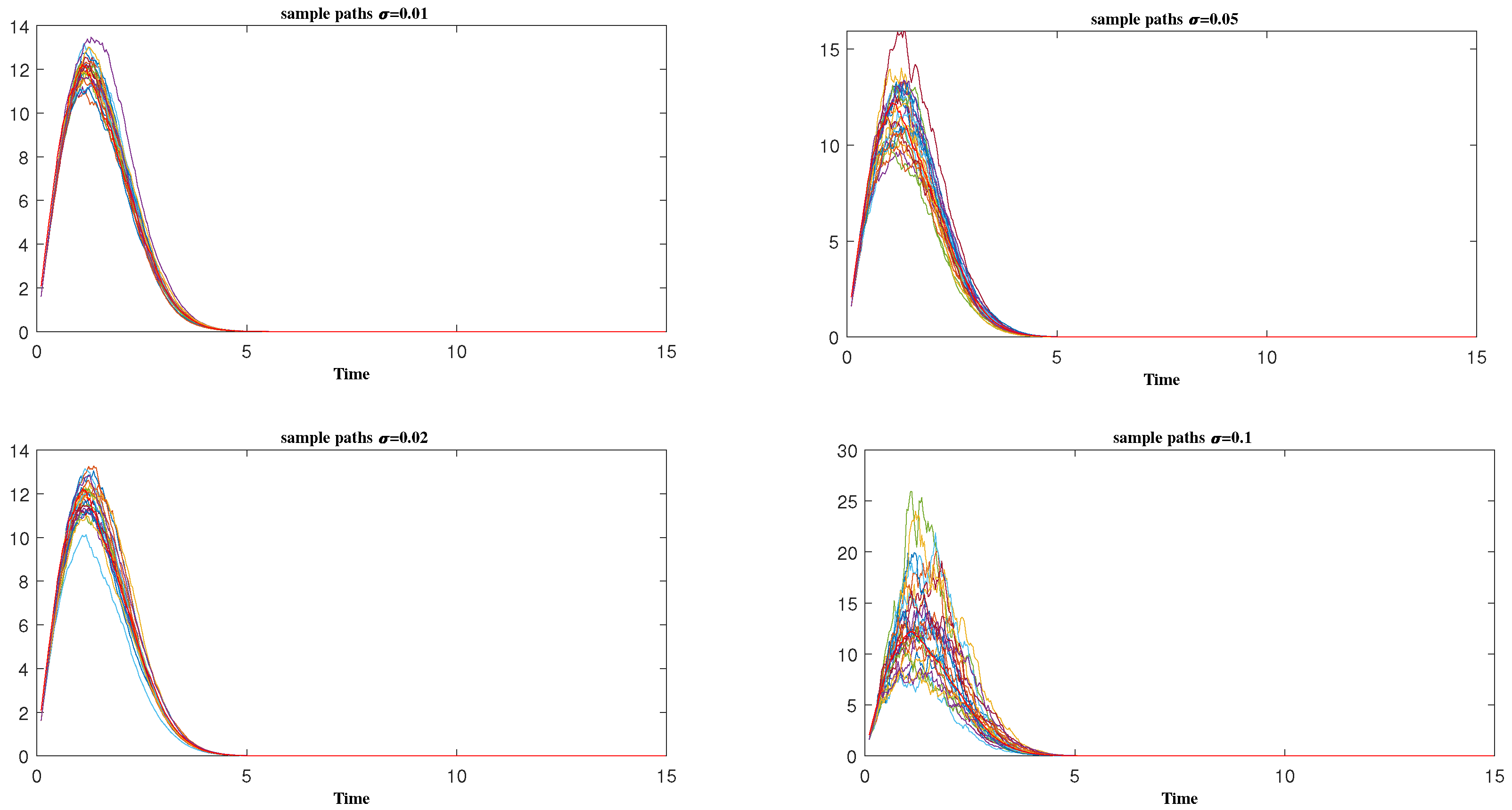
Figure 1. Simulated trajectories for the SRDP and MF ( β = 0.7 ).
Fractalfract 07 00660 g001
Figure 2. The SRDP’s simulated data, as well as the EMF and its ECI.
Fractalfract 07 00660 g002
Figure 3. The SRDP’s simulated data, as well as the ECMF and its ECI.
Fractalfract 07 00660 g003
Figure 4. Observed and predicted values when using the EMF.
Fractalfract 07 00660 g004
Figure 5. Observed and predicted values when using the ECMF.
Fractalfract 07 00660 g005
Table 1. The EM, the std and the CV for β and σ .
β ¯ = 1 M i = 1 M β i std ( β ) = 1 M 1 i = 1 M β i β ¯ 2 1 2 CV ( β ) = std ( β ) β ¯
σ ¯ = 1 M i = 1 M σ i std σ = 1 M 1 i = 1 M σ i σ ¯ 2 1 2 CV σ = std σ σ ¯
Table 2. The parameters estimated, as well as the std and CV of β and σ ( β = 0.5 ).
N β ¯ σ ¯ std ( β ) std ( σ ) CV ( β ) CV ( σ )
1000.4963270.0228910.0048530.0011400.0097780.049805
2000.5224790.0054280.0131470.0005540.0251620.102109
5000.4955570.0105470.0140240.0007630.0283010.072424
Table 3. The MAE, RMSE and the MAPE.
MAE = 1 N i = 2 N x ( t i ) x ^ t i
RMSE = 1 N i = 2 N x ( t i ) x ^ ( t i ) 2
MAPE = 1 N i = 2 N x ( t i ) x ^ ( t i ) x ( t i ) × 100
Table 4. Interpretation of a typical MAPE.
MAPEInterpretation
<10Highly accurate forecasting
20–30Good forecasting
30–50Reasonable forecasting
>50Inaccurate forecasting
Table 5. Performance of fit.
MAERMSEMAPE
0.109250.179313.56523
Table 6. Estimated parameters of the process.
Parameters β ^ σ ^ 2
estimated values0.201740.02124
Table 7. Simulated and forecast values, as well as the EMF, ECMF and ECI.
i x ( i ) EMFECMFECI
12.5316002.5316002.53160[02.53160 02.53160]
210.6431010.6755510.67555[10.46910 10.88499]
318.1054918.1342818.07915[17.72953 18.43385]
424.3301024.4597524.42093[23.94867 24.90004]
529.2681029.3210729.16564[28.60162 29.73784]
632.5767032.5320032.47323[31.84525 33.11032]
733.6632034.0587534.10554[33.44599 34.77466]
833.2841934.0082633.61329[32.96326 34.27275]
931.6657032.6008031.90671[31.28968 32.53268]
1029.1204030.1324429.26814[28.70214 29.84235]
1125.9514926.9339826.02936[25.52600 26.54003]
1222.4932023.3326222.48150[22.04674 22.92257]
1318.3614919.6209818.91509[18.54931 19.28619]
1414.9502016.0363815.00699[14.71678 15.30141]
1512.0474012.7508211.88717[11.65729 12.12038]
1609.2378009.8707109.32617[09.14582 09.50914]
1707.0415007.4440106.96670[06.83197 07.10338]
1805.2021005.4718605.17599[05.07589 05.27754]
1903.7341003.9220903.72873[03.65662 03.80188]
2002.6206002.7422502.61081[02.56032 02.66203]
2101.7638001.8708401.78784[01.75327 01.82292]
22-01.2457201.17444[01.15173 01.19748]
23-00.8097500.76449[00.74971 00.77949]
24-00.5139400.49429[00.48473 00.50399]
Table 8. Observed data, fits and forecast using the EMF and ECMF.
COVID-19 Active CasesEMFECMFECCB
14,02414,02414,024[14,024 14,024]
18,15219,77419,774[18,347 21,281]
22,45725,26823,195[21,522 24,963]
26,39630,43827,052[25,101 29,114]
31,80835,22530,547[28,343 32,875]
35,76839,57535,736[33,158 38,460]
38,38643,44639,266[36,433 42,259]
42,28246,80241,352[38,368 44,504]
46,08149,62244,829[41,595 48,246]
49,49151,89048,188[44,711 51,860]
52,35053,60451,126[47,437 55,022]
55,97154,77053,488[49,629 57,565]
55,98255,40256,617[52,532 60,932]
57,56855,52556,106[52,058 60,382]
58,63155,16857,198[53,071 61,558]
57,02154,36957,782[53,613 62,186]
55,65553,16955,762[51,739 60,012]
52,35351,61354,027[50,129 58,144]
49,61349,75050,463[46,822 54,309]
46,61047,62947,497[44,070 51,117]
40,84545,29844,329[41,131 47,708]
36,88442,80638,598[35,814 41,540]
35,67740,20034,639[32,140 37,279]
35,25537,52433,302[30,899 35,840]
32,74634,81832,713[30,352 35,206]
30,79132,11930,208[28,028 32,510]
27,56029,46028,242[26,204 30,394]
28,25726,86925,136[23,323 27,052]
23,99124,37025,629[23,780 27,582]
22,46221,98321,641[20,079 23,290]
21,56919,72320,152[18,698 21,688]
20,24217,60019,248[17,859 20,715]
19,69415,62317,968[16,672 19,338]
16,01413,79617,390[16,136 18,716]
13,39212,11914,068[13,053 15,140]
11,96110,59111,704[10,859 12,596]
Prediction
-09,20910,400[09,650 11,192]
-07,96609,707[09,007 10,447]
-06,85708,775[08,142 09,444]
-05,87208,012[07,434 08,623]
Disclaimer/Publisher’s Note: The statements, opinions and data contained in all publications are solely those of the individual author(s) and contributor(s) and not of MDPI and/or the editor(s). MDPI and/or the editor(s) disclaim responsibility for any injury to people or property resulting from any ideas, methods, instructions or products referred to in the content.