Exploring Families of Solitary Wave Solutions for the Fractional Coupled Higgs System Using Modified Extended Direct Algebraic Method

Abstract

In this paper, we suggest the modified Extended Direct Algebraic Method (mEDAM) to examine the existence and dynamics of solitary wave solutions in the context of the fractional coupled Higgs system, with Caputo’s fractional derivatives. The method begins with the formulation of nonlinear differential equations using a fractional complex transformation, followed by the derivation of solitary wave solutions. Two-dimensional, Three-dimensional and contour graphs are used to investigate the behavior of traveling wave solutions. The research reveals many families of solitary wave solutions as well as their deep interrelationships and dynamics. These discoveries add to a better understanding of the dynamics of the fractionally coupled Higgs system and have potential applications in areas that use nonlinear Fractional Partial Differential Equations (FPDEs).

1. Introduction

FPDEs are essential mathematical tools for correctly simulating systems with non-local behavior [1], anomalous diffusion [2], and long-range interactions [3]. They are also widely used in the fields of data analysis [4], image and signal processing [5] and materials research [6]. FPDEs are therefore receiving a lot of attention as a result of their capacity to give more accurate modelling of systems.

Because of their intrinsic non-local and non-linear properties, both Partial Differential Equations (PDEs) and FPDEs can pose major obstacles in their solutions. Though they are often employed, numerical approaches, such as finite difference method [7], finite element method [8] and many more [9,10,11,12,13,14,15,16,17], can be computationally costly for complicated FPDEs. When feasible, analytical approaches are chosen since they produce precise results. These techniques employ mathematical approaches to reduce the complexity of the FPDE such that it may be resolved analytically. Analytical techniques are useful because they shed light on the system’s behavior and connections between its variables. They also make it possible to examine unusual circumstances and spot singularities that numerical approaches could overlook. In general, analytical approaches are suggested for solving FPDEs due to their precision, effectiveness, and capacity to offer insightful information about the system under study.

Therefore, the Laplace transform method [18], Fourier transform method [19], Adomian decomposition method [20], direct algebraic method [21], homotopy perturbation method [22], variational iteration method [23] and other analytical techniques have all been employed by researchers to solve FPDEs. Each approach has benefits and drawbacks, and the selection of approach relies on the particular topic being investigated. However, where possible, analytical approaches are preferable over numerical methods because they offer precise solutions and insightful information about how the system behaves.

To construct solitary wave solutions for PDEs and FPDEs, one of the novel analytical methods is mEDAM. The technique entails transforming the FPDE into a nonlinear ODE using the appropriate transformation, which is then resolved using a series form solution. The nonlinear ODE that results from this solution is then utilized to create a set of algebraic equations, which are then solved to get the solitary wave solutions for the FPDE. A soliton, commonly referred to as a solitary wave, is a self-sustaining wave-like solution to certain nonlinear PDEs and FPDEs that retains its shape and speed while traveling with no alteration to its form. Among the different analytical approaches for developing soliton solutions, the mEDAM stands out as the most successful, producing a wider range of soliton solution families. For instance, Sayed et al., have employed mEDAM to construct a number of families of soliton solutions for the three different types of Tzitzeica type PDEs arising in nonlinear optics [24]. Similarly, Yasmin et al., have investigated 32 different families of symmetric soliton solutions for the fractional coupled Konno–Onno system in [25] and 33 families of 131 optical soliton solutions for a fractional perturbed Radhakrishnan-Kundu–Lakshmanan model in [26], respectively, using mEDAM.

The mEDAM is employed in this work to examine solitary wave solutions for the fractional coupled Higgs system. In a relativistic quantum field theory, the fractional coupled Higgs system is a mathematical model that describes the dynamics of two scalar fields. In this system, the interaction of the two scalar fields results in intricate behavior. We considered this system in fractional form to characterize anomalous diffusion and non-local behavior, which are known to occur in many physical systems. By accounting for non-local influences on the system, fractional derivatives allow for more detailed models of solitons’ behavior. The mathematical form of this system is given as follows [27]:

$$\left\{\begin{array}{c}{D}_t^{\gamma }\left(D_t^{\gamma }u\right)-D_x^{\delta }\left(D_x^{\delta }u\right)+{\left|u\right|}^{2}u-2uv=0,\hfill \\ D_t^{\gamma }\left(D_t^{\gamma }v\right)+D_x^{\delta }\left(D_x^{\delta }v\right)-D_x^{\delta }(D_x^{\delta }{\left|u\right|}^2)=0.\hfill \end{array}\right.$$

(1)

where $0<\gamma ,\delta \le 1$ and $u=u(x,t)$, and $v=v(x,t)$. It should be noted that the proposed model in [27] is time-fractional; however, we have generalized the model by replacing the space derivative by Caputo’s fractional derivative. The system is composed of two equations: the first represents how the amplitude and phase of the soliton have changed over time, and the second defines how the background field has changed over time. The system shows a wide range of events, including solitons production, scattering, and formation. The fractional Higgs system is especially important in particle physics since it controls particle interactions and behavior, including how particles are assigned mass. As a result of the system’s symmetry breakdown, topological solitons, and nontrivial scattering amplitudes, much theoretical and experimental study has been conducted.

Several researchers have already used various analytical methods to investigate the coupled Higgs system in integer and fractional orders. The Sin–Gorden method was utilized by Rezazadeh et al. in [27] to solve the coupled Higgs system in time-fractional form. Jabbari et al., obtained precise solutions to the coupled Higgs system (in integer order) and the Maccari system using He’s semi-inverse technique and a simple $\left(\frac{G^{\prime }}{G}\right)$-expansion method [28]. Similar to this, Atas et al. [29] identified invariant optical soltons as coupled-Higgs equation solutions. The exp-expansion method was utilized by Seadway et al. [30] to get traveling wave solutions for the given system. Mu and Qin provided Rogue Waves for the Coupled Schrödinger–Boussinesq Equation and the Coupled Higgs Equation using the Hirota technique [31].

The fractional derivatives present in (1) are defined using Caputo’s derivative operator. This operator with some of its properties is defined as follows [32]:

$${}^C{D}_t^{\alpha }f\left(t\right)=\frac{1}{\mathrm{\Gamma }(n-\alpha )}{\int }_0^t\frac{\frac{{\partial }^{n}f\left(s\right)}{\partial s^n}}{{(t-s)}^{\alpha -n+1}}ds,$$

(2)

$$D_y^{\alpha }{y}^p=\frac{\mathrm{\Gamma }(1+p)}{\mathrm{\Gamma }(1+p-\alpha )}{y}^{p-\alpha },$$

(3)

$$D_y^{\alpha }g\left[h\left(y\right)\right]=g_h^{\prime }\left(h\left(y\right)\right)D_y^{\alpha }h\left(y\right)=D_h^{\alpha }g\left(h\left(y\right)\right){\left[h^{\prime }\left(y\right)\right]}^{\alpha }0<\alpha \le 1,$$

(4)

where $\alpha$ is the order of the derivative, $g\left(t\right)$ and $h\left(t\right)$ are the functions to be differentiated, n is the smallest integer greater than or equal to $\alpha$, and $\mathrm{\Gamma }(·)$ is the Gamma function.

2. Methodology of mEDAM

This section outlines the modified EDAM technique. Consider the FPDE of the form [25,26]:

$$P(w,{\partial }_t^{\alpha }w,{\partial }_{y_1}^{\beta }w,{\partial }_{y_2}^{\gamma }w,w^2,\dots )=0,0<\alpha ,\beta ,\gamma \le 1,$$

(5)

where w is a function of $y_1,y_2,y_3,\dots ,y_r$ and t.

The below steps are used to solve Equation (5):

1.

We start by transforming the variables $w(y_1,y_2,y_3,ldots,y_r)$ into $W\left(xi\right)$, where $\xi$ is specified in a variety of ways. Equation (5) is changed by this transformation into a nonlinear ODE of the following form:

$$Q(W,W^{\prime }W,W^{\prime },\cdots )=0,$$

(6)

where W in (6) has derivatives with respect to $\xi$. Equation (6) may be integrated once or more times to obtain the constant(s) of integration.

2.

Next, we assume that (6) has the following solution:

$$W\left(\xi \right)=\sum _{l=-m}^m{d}_l{\left(Z\left(\xi \right)\right)}^l,$$

(7)

where $d_l(l=-m,\dots ,0,1,2,\dots ,m)$ are constants to be determined, and $Z\left(\xi \right)$ is the general solution of the following ODE:

$$Z^{\prime }\left(\xi \right)=ln\left(A\right)(a+bZ\left(\xi \right)+c{\left(Z\left(\xi \right)\right)}^2),$$

(8)

where $a,b$ and c are constants and $A\ne 0,1$.

3.

Establishing the homogeneous balance between the greatest nonlinear term and the highest-order derivative in (6) yields the positive integer m given in (7). More precisely the balance number can be estimated by using the given two formulas [33]:

$$D\left(\frac{d^{k}W}{d{\xi }^k}\right)=m+k\mathrm{and}D\left(W^j{\left(\frac{d^{k}W}{d{\xi }^k}\right)}^l\right)=mj+l(k+m),$$

where D stands for degree of $W\left(\xi \right)$ as $D\left[W\right(\xi \left)\right]=m$ and $j,k$ and l are positive integers.

4.

Then, we put (7) into (6) or the equation that comes from integrating (6), and arrange all of the terms of $Z\left(\xi \right)$ in the same order. The subsequent polynomial’s coefficients are then all set to zero, resulting in a system of algebraic equations for $d_l(l=-m,\dots ,0,1,2,\dots ,m)$ and additional parameters.

5.

To solve this set of algebraic equations, we use MAPLE.

6.

The analytical solutions to (5) are then obtained by determining the unknown values and inserting them into (7) together with the $Z\left(\xi \right)$(solution of Equation (8)). Using the general solution of (8), we may produce the following families of solutions.

Family 1.

For $M<0$ and $c\ne 0$,

$$Z_1\left(\xi \right)=-\frac{b}{2c}+\frac{\sqrt{-M}{\tan }_A\left(1/2\sqrt{-M}\xi \right)}{2c},$$

$$Z_2\left(\xi \right)=-\frac{b}{2c}-\frac{\sqrt{-M}{\cot }_A\left(1/2\sqrt{-M}\xi \right)}{2c},$$

$$Z_3\left(\xi \right)=-\frac{b}{2c}+\frac{\sqrt{-M}\left({\tan }_A\left(\sqrt{-M}\xi \right)\pm \left(\sqrt{pq}{\sec }_A\left(\sqrt{-M}\xi \right)\right)\right)}{2c},$$

$$Z_4\left(\xi \right)=-\frac{b}{2c}-\frac{\sqrt{-M}\left({\cot }_A\left(\sqrt{-M}\xi \right)\pm \left(\sqrt{pq}{\csc }_A\left(\sqrt{-M}\xi \right)\right)\right)}{2c},$$

and

$$Z_5\left(\xi \right)=-\frac{b}{2c}+\frac{\sqrt{-M}\left({\tan }_A\left(1/4\sqrt{-M}\xi \right)-{\cot }_A\left(1/4\sqrt{-M}\xi \right)\right)}{4c}.$$

Family 2.

For $M>0$ and $c\ne 0$,

$$Z_6\left(\xi \right)=-\frac{b}{2c}-\frac{\sqrt{M}{\tanh }_A\left(1/2\sqrt{M}\xi \right)}{2c},$$

$$Z_7\left(\xi \right)=-\frac{b}{2c}-\frac{\sqrt{M}{\coth }_A\left(1/2\sqrt{M}\xi \right)}{2c},$$

$$Z_8\left(\xi \right)=-\frac{b}{2c}-\frac{\sqrt{Z}\left({\tanh }_A\left(\sqrt{M}\xi \right)\pm \left(\sqrt{pq}{\mathit{sech}}_{\mathit{A}}\left(\sqrt{M}\xi \right)\right)\right)}{2c},$$

$$Z_9\left(\xi \right)=-\frac{b}{2c}-\frac{\sqrt{M}\left({\coth }_A\left(\sqrt{M}\xi \right)\pm \left(\sqrt{pq}{\mathit{csch}}_{\mathit{A}}\left(\sqrt{M}\xi \right)\right)\right)}{2c},$$

and

$$Z_{10}\left(\xi \right)=-\frac{b}{2c}-\frac{\sqrt{M}\left({\tanh }_A\left(1/4\sqrt{M}\xi \right)-{\coth }_A\left(1/4\sqrt{M}\xi \right)\right)}{4c}.$$

Family 3.

For $ac>0$ and $b=0$,

$$Z_{11}\left(\xi \right)=\sqrt{\frac{a}{c}}{\tan }_A\left(\sqrt{ac}\xi \right),$$

$$Z_{12}\left(\xi \right)=-\sqrt{\frac{a}{c}}{\cot }_A\left(\sqrt{ac}\xi \right),$$

$$Z_{13}\left(\xi \right)=\sqrt{\frac{a}{c}}\left({\tan }_A\left(2\sqrt{ac}\xi \right)\pm \left(\sqrt{pq}{\sec }_A\left(2\sqrt{ac}\xi \right)\right)\right),$$

$$Z_{14}\left(\xi \right)=-\sqrt{\frac{a}{c}}\left({\cot }_A\left(2\sqrt{ac}\xi \right)\pm \left(\sqrt{pq}{\csc }_A\left(2\sqrt{ac}\xi \right)\right)\right),$$

and

$$Z_{15}\left(\xi \right)=\frac{1}{2}\sqrt{\frac{a}{c}}\left({\tan }_A\left(1/2\sqrt{ac}\xi \right)-{\cot }_A\left(1/2\sqrt{ac}\xi \right)\right).$$

Family 4.

For $ac<0$ and $b=0$, then

$$Z_{16}\left(\xi \right)=-\sqrt{-\frac{a}{c}}{\tanh }_A\left(\sqrt{-ac}\xi \right),$$

$$Z_{17}\left(\xi \right)=-\sqrt{-\frac{a}{c}}{\coth }_A\left(\sqrt{-ac}\xi \right)$$

$$Z_{18}\left(\xi \right)=-\sqrt{-\frac{a}{c}}\left({\tanh }_A\left(2\sqrt{-ac}\xi \right)\pm \left(i\sqrt{pq}{\mathit{sech}}_{\mathit{A}}\left(2\sqrt{-ac}\xi \right)\right)\right),$$

$$Z_{19}\left(\xi \right)=-\sqrt{-\frac{a}{c}}\left({\coth }_A\left(2\sqrt{-ac}\xi \right)\pm \left(\sqrt{pq}{\mathit{csch}}_{\mathit{A}}\left(2\sqrt{-ac}\xi \right)\right)\right),$$

and

$$Z_{20}\left(\xi \right)=-\frac{1}{2}\sqrt{-\frac{a}{c}}\left({\tanh }_A\left(1/2\sqrt{-ac}\xi \right)+{\coth }_A\left(1/2\sqrt{-ac}\xi \right)\right).$$

Family 5.

For $c=a$ and $b=0$,

$$Z_{21}\left(\xi \right)={\tan }_A\left(a\xi \right),$$

$$Z_{22}\left(\xi \right)=-{\cot }_A\left(a\xi \right),$$

$$Z_{23}\left(\xi \right)={\tan }_A\left(2a\xi \right)\pm \left(\sqrt{pq}{\sec }_A\left(2a\xi \right)\right),$$

$$Z_{24}\left(\xi \right)=-{\cot }_A\left(2a\xi \right)\pm \left(\sqrt{pq}{\csc }_A\left(2a\xi \right)\right),$$

and

$$Z_{25}\left(\xi \right)=\frac{1}{2}{\tan }_A\left(1/2a\xi \right)-1/2{\cot }_A\left(1/2a\xi \right).$$

Family 6.

For $c=-a$ and $b=0$,

$$Z_{26}\left(\xi \right)=-{\tanh }_A\left(a\xi \right),$$

$$Z_{27}\left(\xi \right)=-{\coth }_A\left(a\xi \right),$$

$$Z_{28}\left(\xi \right)=-{\tanh }_A\left(2a\xi \right)\pm \left(i\sqrt{pq}{\mathit{sech}}_{\mathit{A}}\left(2a\xi \right)\right),$$

$$Z_{29}\left(\xi \right)=-{\coth }_A\left(2a\xi \right)\pm \left(\sqrt{pq}{\mathit{csch}}_{\mathit{A}}\left(2a\xi \right)\right),$$

and

$$Z_{30}\left(\xi \right)=-\frac{1}{2}{\tanh }_A\left(1/2a\xi \right)-1/2{\coth }_A\left(1/2a\xi \right).$$

Family 7.

For $M=0$,

$$Z_{31}\left(\xi \right)=-2\frac{a\left(b\xi \ln \left(A\right)+2\right)}{b^2\xi \ln \left(A\right)}.$$

Family 8.

For $b=\lambda$, $a=n\lambda (n\ne 0)$ and $c=0$,

$$Z_{32}\left(\xi \right)=A^{\lambda \xi }-n.$$

Family 9.

For $b=c=0$,

$$Z_{33}\left(\xi \right)=a\xi \ln \left(A\right).$$

Family 10.

For $b=a=0$,

$$Z_{34}\left(\xi \right)=-\frac{1}{c\xi \ln \left(A\right)}.$$

Family 11.

For $a=0$, $b\ne 0$ and $c\ne 0$,

$$Z_{35}\left(\xi \right)=-\frac{pb}{c\left({\cosh }_A\left(b\xi \right)-{\sinh }_A\left(b\xi \right)+p\right)},$$

and

$$Z_{36}\left(\xi \right)=-\frac{b\left({\cosh }_A\left(b\xi \right)+{\sinh }_A\left(b\xi \right)\right)}{c\left({\cosh }_A\left(b\xi \right)+{\sinh }_A\left(b\xi \right)+q\right)}.$$

Family 12.

For $b=\lambda$, $c=n\lambda (n\ne 0)$ and $a=0$,

$$Z_{37}\left(\xi \right)=\frac{p{A}^{\lambda \xi }}{p-nq{A}^{\lambda \xi }}.$$

where $M=b^2-4ac$ and $p,q>0$ and are referred to as deformation parameters. The generalized trigonometric and hyperbolic functions are described as follows:

$$\begin{array}{cc}\hfill & {\cos }_A\left(\xi \right)=\frac{p{A}^{i\xi }+q{A}^{-i\xi }}{2},{\sin }_A\left(\xi \right)=\frac{p{A}^{i\xi }-q{A}^{-i\xi }}{2i},\hfill \\ \hfill & {\cot }_A\left(\xi \right)=\frac{{\cos }_A\left(\xi \right)}{{\sin }_A\left(\xi \right)},{\tan }_A\left(\xi \right)=\frac{{\sin }_A\left(\xi \right)}{{\cos }_A\left(\xi \right)},\hfill \\ \hfill & {\csc }_A\left(\xi \right)=\frac{1}{{\sin }_A\left(\xi \right)},{\sec }_A\left(\xi \right)=\frac{1}{{\cos }_A\left(\xi \right)}.\hfill \end{array}$$

Similarly,

$$\begin{array}{cc}\hfill & {\cosh }_A\left(\xi \right)=\frac{p{A}^{\xi }+q{A}^{-\xi }}{2},{\sinh }_A\left(\xi \right)=\frac{p{A}^{\xi }-q{A}^{-\xi }}{2},\hfill \\ \hfill & {\coth }_A\left(\xi \right)=\frac{{\cosh }_A\left(\xi \right)}{{\sinh }_A\left(\xi \right)},{\tanh }_A\left(\xi \right)=\frac{{\sinh }_A\left(\xi \right)}{{\cosh }_A\left(\xi \right)},\hfill \\ \hfill & {\mathrm{csch}}_A\left(\xi \right)=\frac{1}{{\sinh }_A\left(\xi \right)},{\mathrm{sech}}_A\left(\xi \right)=\frac{1}{{\cosh }_A\left(\xi \right)}.\hfill \end{array}$$

3. Execution of the Approach

In the present section, we use the suggested method for solving the fractional coupled Higgs system (1). We offer a transformation so that this approach may be expanded to solve (1):

$$\begin{array}{cc}\hfill & u(x,t)=U\left(\xi \right)e^{i\theta },v(x,t)=V\left(\xi \right),\hfill \\ \hfill & where\xi =\frac{x^{\delta }}{\mathrm{\Gamma }(1+\delta )}+\frac{k{t}^{\gamma }}{\mathrm{\Gamma }(1+\gamma )},\theta =\frac{a_1{x}^{\delta }}{\mathrm{\Gamma }(1+\delta )}+\frac{b_1{t}^{\gamma }}{\mathrm{\Gamma }(1+\gamma )},\hfill \end{array}$$

(9)

in (9), the soliton’s phase component is denoted by $\theta (x,t)$, its wavenumber is denoted by $b_1$, and its velocity is denoted by $a_1$. When (9) is substituted into (1), we have

$$\begin{array}{cc}\hfill & (k^2-1)U^{\prime \prime }+(a_1^2-b_1^2)U-2UV+U^3=0,\hfill \\ \hfill & (k^2+1)V^{\prime \prime }-2{\left(U^{\prime }\right)}^2-2U{U}^{\prime \prime }=0.\hfill \end{array}$$

(10)

Ignoring the integration constant and integrating the second equation in (10), we get

$$V(1+k^2)=U^2.$$

(11)

Putting (11) into the first equation of (10) and integrating gives us

$$(k^4-1)U^{\prime \prime }+(a_1^2-b_1^2)(k^2+1)U+(k^2-1)U^3=0,$$

(12)

where prime represents differentiation with respect to $\xi$. $m=1$ is obtained by balancing the terms of $U^{\prime \prime }$ and $U^3$ in (12).

Implementation of mEDAM to the Problem

To solve the NODE in (12) generated from the fractional coupled Higgs system using mEDAM, put $m=1$ in (7). Thus, we have

$$U\left(\xi \right)=\sum _{i=-1}^1{d}_i{\left(Z\left(\xi \right)\right)}^i=d_{-1}{\left(Z\left(\xi \right)\right)}^{-1}+d_0+d_1{\left(Z\left(\xi \right)\right)}^1,$$

(13)

where $d_{-1}$, $d_0$ and $d_1$ are coefficients that will be determined.

With the help of (8), we insert (13) into (12), which creates a polynomial in $Z\left(\xi \right)$ by collecting the terms with the same power of $Z\left(\xi \right)$. By equating the coefficients of the polynomial to zero, we get a system of nonlinear algebraic equations. We use Maple to solve the system, leading to the identification of the following two distinct cases of solutions:

Case 1:

$$\begin{array}{cc}\hfill & d_1=2\sqrt{\frac{-M{\left(\ln \left(A\right)\right)}^2-\mathrm{\Omega }}{M}}c,d_{-1}=0,d_0=\sqrt{\frac{-M{\left(\ln \left(A\right)\right)}^2-\mathrm{\Omega }}{M}}b,k=\sqrt{\frac{M{\left(\ln \left(A\right)\right)}^2+2\mathrm{\Omega }}{M{\left(\ln \left(A\right)\right)}^2}}.\hfill \end{array}$$

(14)

Case 2:

$$\begin{array}{cc}\hfill & d_1=0,d_{-1}=2\sqrt{\frac{-M{\left(\ln \left(A\right)\right)}^2-\mathrm{\Omega }}{M}}a,d_0=\sqrt{\frac{-M{\left(\ln \left(A\right)\right)}^2-\mathrm{\Omega }}{M}}b,k=\sqrt{\frac{M{\left(\ln \left(A\right)\right)}^2+2\mathrm{\Omega }}{M{\left(\ln \left(A\right)\right)}^2}},\hfill \end{array}$$

(15)

where $\mathrm{\Omega }=a_1^2-b_1^2$ and $M=b^2-4ac$.

Assuming Case 1, we get the following families of solutions:

Family 13.

When $M<0$ and $a,b,c\ne 0$, then the following set of equations presents the corresponding family of solitary wave solutions: 

$$\begin{array}{cc}\hfill U_1(x,t)& =\sqrt{-\frac{Z{\left(\ln \left(A\right)\right)}^2+\mathrm{\Omega }}{Z}}\sqrt{-Z}{\tan }_A\left(1/2\sqrt{-Z}\xi \right).\hfill \end{array}$$

(16)

Using (9) and (11), the subsequent solitary wave solutions are obtained for (1) as

$$\begin{array}{cc}\hfill u_1(x,t)& =e^{i\theta }\left(\sqrt{-\frac{Z{\left(\ln \left(A\right)\right)}^2+\mathrm{\Omega }}{Z}}\sqrt{-Z}{\tan }_A\left(1/2\sqrt{-Z}\xi \right)\right),\hfill \end{array}$$

(17)

and

$$\begin{array}{cc}\hfill v_1(x,t)& =\frac{1}{1+k^2}{\left(\sqrt{-\frac{Z{\left(\ln \left(A\right)\right)}^2+\mathrm{\Omega }}{Z}}\sqrt{-Z}{\tan }_A\left(1/2\sqrt{-Z}\xi \right)\right)}^2,\hfill \end{array}$$

(18)

$$\begin{array}{cc}\hfill U_2(x,t)& =-\sqrt{-\frac{M{\left(\ln \left(A\right)\right)}^2+\mathrm{\Omega }}{M}}\sqrt{-M}{\cot }_A\left(1/2\sqrt{-M}\xi \right).\hfill \end{array}$$

(19)

Utilizing (9) and (11), the subsequent solitary wave solutions are obtained for (1) as

$$\begin{array}{cc}\hfill u_2(x,t)& =e^{i\theta }\left(-\sqrt{-\frac{M{\left(\ln \left(A\right)\right)}^2+\mathrm{\Omega }}{M}}\sqrt{-M}{\cot }_A\left(1/2\sqrt{-M}\xi \right)\right),\hfill \end{array}$$

(20)

and

$$\begin{array}{cc}\hfill v_2(x,t)& =\frac{1}{1+k^2}{\left(-\sqrt{-\frac{M{\left(\ln \left(A\right)\right)}^2+\mathrm{\Omega }}{M}}\sqrt{-M}{\cot }_A\left(1/2\sqrt{-M}\xi \right)\right)}^2,\hfill \end{array}$$

(21)

$$\begin{array}{cc}\hfill U_3(x,t)& =\frac{\sqrt{M{\left(\ln \left(A\right)\right)}^2+\mathrm{\Omega }}\left({\sin }_A\left(\sqrt{-M}\xi \right)+\sqrt{pq}\right)}{{\cos }_A\left(\sqrt{-M}\xi \right)}.\hfill \end{array}$$

(22)

Using (9) and (11), the subsequent solitary wave solutions are obtained for (1) as

$$\begin{array}{cc}\hfill u_3(x,t)& =e^{i\theta }\left(\frac{\sqrt{M{\left(\ln \left(A\right)\right)}^2+\mathrm{\Omega }}\left({\sin }_A\left(\sqrt{-M}\xi \right)+\sqrt{pq}\right)}{{\cos }_A\left(\sqrt{-M}\xi \right)}\right),\hfill \end{array}$$

(23)

and

$$\begin{array}{cc}\hfill v_3(x,t)& =\frac{1}{1+k^2}{\left(\frac{\sqrt{M{\left(\ln \left(A\right)\right)}^2+\mathrm{\Omega }}\left({\sin }_A\left(\sqrt{-M}\xi \right)+\sqrt{pq}\right)}{{\cos }_A\left(\sqrt{-M}\xi \right)}\right)}^2,\hfill \end{array}$$

(24)

$$\begin{array}{cc}\hfill U_4(x,t)& =-\frac{\sqrt{M{\left(\ln \left(A\right)\right)}^2+\mathrm{\Omega }}\left({\cos }_A\left(\sqrt{-M}\xi \right)+\sqrt{pq}\right)}{{\sin }_A\left(\sqrt{-M}\xi \right)}.\hfill \end{array}$$

(25)

Using (9) and (11), the subsequent solitary wave solutions are obtained for (1) as

$$\begin{array}{cc}\hfill u_4(x,t)& =e^{i\theta }\left(-\frac{\sqrt{M{\left(\ln \left(A\right)\right)}^2+\mathrm{\Omega }}\left({\cos }_A\left(\sqrt{-M}\xi \right)+\sqrt{pq}\right)}{{\sin }_A\left(\sqrt{-M}\xi \right)}\right),\hfill \end{array}$$

(26)

and

$$\begin{array}{cc}\hfill v_4(x,t)& =\frac{1}{1+k^2}{\left(-\frac{\sqrt{M{\left(\ln \left(A\right)\right)}^2+\mathrm{\Omega }}\left({\cos }_A\left(\sqrt{-M}\xi \right)+\sqrt{pq}\right)}{{\sin }_A\left(\sqrt{-M}\xi \right)}\right)}^2,\hfill \end{array}$$

(27)

and

$$\begin{array}{cc}\hfill U_5(x,t)& =-1/2\frac{\sqrt{M{\left(\ln \left(A\right)\right)}^2+\mathrm{\Omega }}\left(-1+2{\left({\cos }_A\left(1/4\sqrt{-M}\xi \right)\right)}^2\right)}{{\cos }_A\left(1/4\sqrt{-M}\xi \right){\sin }_A\left(1/4\sqrt{-M}\xi \right)}.\hfill \end{array}$$

(28)

Using (9) and (11), the subsequent solitary wave solutions are obtained for (1) as

$$\begin{array}{cc}\hfill u_5(x,t)& =e^{i\theta }\left(-1/2\frac{\sqrt{M{\left(\ln \left(A\right)\right)}^2+\mathrm{\Omega }}\left(-1+2{\left({\cos }_A\left(1/4\sqrt{-M}\xi \right)\right)}^2\right)}{{\cos }_A\left(1/4\sqrt{-M}\xi \right){\sin }_A\left(1/4\sqrt{-M}\xi \right)}\right),\hfill \end{array}$$

(29)

and

$$\begin{array}{cc}\hfill v_5(x,t)& =\frac{1}{1+k^2}{\left(-1/2\frac{\sqrt{M{\left(\ln \left(A\right)\right)}^2+\mathrm{\Omega }}\left(-1+2{\left({\cos }_A\left(1/4\sqrt{-M}\xi \right)\right)}^2\right)}{{\cos }_A\left(1/4\sqrt{-M}\xi \right){\sin }_A\left(1/4\sqrt{-M}\xi \right)}\right)}^2.\hfill \end{array}$$

(30)

Family 14.

For $M>0$ and $a,b,c\ne 0$, then the following set of equations presents the corresponding family of solitary wave solutions:

$$\begin{array}{cc}\hfill U_6(x,t)& =-\sqrt{M{\left(\ln \left(A\right)\right)}^2+\mathrm{\Omega }}{\tanh }_A\left(1/2\sqrt{M}\xi \right).\hfill \end{array}$$

(31)

Utilizing (9) and (11), the subsequent solitary wave solutions are obtained for (1) as

$$\begin{array}{cc}\hfill u_6(x,t)& =e^{i\theta }\left(-\sqrt{M{\left(\ln \left(A\right)\right)}^2+\mathrm{\Omega }}{\tanh }_A\left(1/2\sqrt{M}\xi \right)\right),\hfill \end{array}$$

(32)

and

$$\begin{array}{cc}\hfill v_6(x,t)& =\frac{1}{1+k^2}{\left(-\sqrt{M{\left(\ln \left(A\right)\right)}^2+\mathrm{\Omega }}{\tanh }_A\left(1/2\sqrt{M}\xi \right)\right)}^2,\hfill \end{array}$$

(33)

$$\begin{array}{cc}\hfill U_7(x,t)& =-\sqrt{M{\left(\ln \left(A\right)\right)}^2+\mathrm{\Omega }}{\coth }_A\left(1/2\sqrt{M}\xi \right).\hfill \end{array}$$

(34)

Utilizing (9) and (11), the subsequent solitary wave solutions are obtained for (1) as

$$\begin{array}{cc}\hfill u_7(x,t)& =e^{i\theta }\left(-\sqrt{M{\left(\ln \left(A\right)\right)}^2+\mathrm{\Omega }}{\coth }_A\left(1/2\sqrt{M}\xi \right)\right),\hfill \end{array}$$

(35)

and

$$\begin{array}{cc}\hfill v_7(x,t)& =\frac{1}{1+k^2}{\left(-\sqrt{M{\left(\ln \left(A\right)\right)}^2+\mathrm{\Omega }}{\coth }_A\left(1/2\sqrt{M}\xi \right)\right)}^2,\hfill \end{array}$$

(36)

$$\begin{array}{cc}\hfill U_8(x,t)& =-\frac{\sqrt{M{\left(\ln \left(A\right)\right)}^2+\mathrm{\Omega }}\left({\sinh }_A\left(\sqrt{M}\xi \right)+\sqrt{pq}\right)}{{\cosh }_A\left(\sqrt{M}\xi \right)}.\hfill \end{array}$$

(37)

Utilizing (9) and (11), the subsequent solitary wave solutions are obtained for (1) as

$$\begin{array}{cc}\hfill u_8(x,t)& =e^{i\theta }\left(-\frac{\sqrt{M{\left(\ln \left(A\right)\right)}^2+\mathrm{\Omega }}\left({\sinh }_A\left(\sqrt{M}\xi \right)+\sqrt{pq}\right)}{{\cosh }_A\left(\sqrt{M}\xi \right)}\right),\hfill \end{array}$$

(38)

and

$$\begin{array}{cc}\hfill v_8(x,t)& =\frac{1}{1+k^2}{\left(-\frac{\sqrt{M{\left(\ln \left(A\right)\right)}^2+\mathrm{\Omega }}\left({\sinh }_A\left(\sqrt{M}\xi \right)+\sqrt{pq}\right)}{{\cosh }_A\left(\sqrt{M}\xi \right)}\right)}^2,\hfill \end{array}$$

(39)

$$\begin{array}{cc}\hfill U_9(x,t)& =-\frac{\sqrt{M{\left(\ln \left(A\right)\right)}^2+\mathrm{\Omega }}\left({\cosh }_A\left(\sqrt{M}\xi \right)+\sqrt{pq}\right)}{{\sinh }_A\left(\sqrt{M}\xi \right)}.\hfill \end{array}$$

(40)

Utilizing (9) and (11), the subsequent solitary wave solutions are obtained for (1) as

$$\begin{array}{cc}\hfill u_9(x,t)& =e^{i\theta }\left(-\frac{\sqrt{M{\left(\ln \left(A\right)\right)}^2+\mathrm{\Omega }}\left({\cosh }_A\left(\sqrt{M}\xi \right)+\sqrt{pq}\right)}{{\sinh }_A\left(\sqrt{M}\xi \right)}\right),\hfill \end{array}$$

(41)

and

$$\begin{array}{cc}\hfill v_9(x,t)& =\frac{1}{1+k^2}{\left(-\frac{\sqrt{M{\left(\ln \left(A\right)\right)}^2+\mathrm{\Omega }}\left({\cosh }_A\left(\sqrt{M}\xi \right)+\sqrt{pq}\right)}{{\sinh }_A\left(\sqrt{M}\xi \right)}\right)}^2,\hfill \end{array}$$

(42)

and

$$\begin{array}{cc}\hfill U_{10}(x,t)& =1/2\frac{\sqrt{M{\left(\ln \left(A\right)\right)}^2+\mathrm{\Omega }}}{{\cosh }_A\left(1/4\sqrt{M}\xi \right){\sinh }_A\left(1/4\sqrt{M}\xi \right)}.\hfill \end{array}$$

(43)

Utilizing (9) and (11), the subsequent solitary wave solutions are obtained for (1) as

$$\begin{array}{cc}\hfill u_{10}(x,t)& =e^{i\theta }\left(1/2\frac{\sqrt{M{\left(\ln \left(A\right)\right)}^2+\mathrm{\Omega }}}{{\cosh }_A\left(1/4\sqrt{M}\xi \right){\sinh }_A\left(1/4\sqrt{M}\xi \right)}\right),\hfill \end{array}$$

(44)

and

$$\begin{array}{cc}\hfill v_{10}(x,t)& =\frac{1}{1+k^2}{\left(1/2\frac{\sqrt{M{\left(\ln \left(A\right)\right)}^2+\mathrm{\Omega }}}{{\cosh }_A\left(1/4\sqrt{M}\xi \right){\sinh }_A\left(1/4\sqrt{M}\xi \right)}\right)}^2.\hfill \end{array}$$

(45)

Family 15.

For $ca>0$ and $b=0$, the following set of equations presents the corresponding family of solitary wave solutions: 

$$\begin{array}{cc}\hfill & U_{11}(x,t)=\sqrt{-(4{\left(\ln \left(A\right)\right)}^{2}ca-\mathrm{\Omega })}{\tan }_A\left(\sqrt{ca}\xi \right).\hfill \end{array}$$

(46)

Utilizing (9) and (11), the subsequent solitary wave solutions are obtained for (1) as

$$\begin{array}{c}\hfill u_{11}(x,t)=e^{i\theta }\left(\sqrt{-(4{\left(\ln \left(A\right)\right)}^{2}ca-\mathrm{\Omega })}{\tan }_A\left(\sqrt{ca}\xi \right)\right),\end{array}$$

(47)

and

$$\begin{array}{c}\hfill v_{11}(x,t)=\frac{1}{1+k^2}{\left(\sqrt{-(4{\left(\ln \left(A\right)\right)}^{2}ca-\mathrm{\Omega })}{\tan }_A\left(\sqrt{ca}\xi \right)\right)}^2,\end{array}$$

(48)

$$\begin{array}{cc}\hfill U_{12}(x,t)& =-\sqrt{-(4{\left(\ln \left(A\right)\right)}^{2}ca-\mathrm{\Omega })}{\cot }_A\left(\sqrt{ca}\xi \right).\hfill \end{array}$$

(49)

Utilizing (9) and (11), the subsequent solitary wave solutions are obtained for (1) as

$$\begin{array}{c}\hfill u_{12}(x,t)=e^{i\theta }(-\sqrt{-(4{\left(\ln \left(A\right)\right)}^{2}ca-\mathrm{\Omega })}{\cot }_A\left(\sqrt{ca}\xi \right)),\end{array}$$

(50)

and

$$\begin{array}{cc}\hfill v_{12}(x,t)& =\frac{1}{1+k^2}{(-\sqrt{-(4{\left(\ln \left(A\right)\right)}^{2}ca-\mathrm{\Omega })}{\cot }_A\left(\sqrt{ca}\xi \right))}^2,\hfill \end{array}$$

(51)

$$\begin{array}{cc}\hfill U_{13}(x,t)& =\sqrt{-(4{\left(\ln \left(A\right)\right)}^{2}ca-\mathrm{\Omega })}\times \hfill \\ \hfill & \left({\tan }_A\left(2\sqrt{ca}\xi \right)\pm \left(\sqrt{pq}{\sec }_A\left(2\sqrt{ca}\xi \right)\right)\right).\hfill \end{array}$$

(52)

Utilizing (9) and (11), the subsequent solitary wave solutions are obtained for (1) as

$$\begin{array}{cc}\hfill u_{13}(x,t)& =e^{i\theta }(\sqrt{-(4{\left(\ln \left(A\right)\right)}^{2}ca-\mathrm{\Omega })}\times \hfill \\ \hfill & \left({\tan }_A\left(2\sqrt{ca}\xi \right)\pm \left(\sqrt{pq}{\sec }_A\left(2\sqrt{ca}\xi \right)\right)\right)),\hfill \end{array}$$

(53)

and

$$\begin{array}{cc}\hfill v_{13}(x,t)& =\frac{1}{1+k^2}(\sqrt{-(4{\left(\ln \left(A\right)\right)}^{2}ca-\mathrm{\Omega })}\times \hfill \\ \hfill & \left({\tan }_A\left(2\sqrt{ca}\xi \right)\pm \left(\sqrt{pq}{\sec }_A\left(2\sqrt{ca}\xi \right)\right)\right){)}^2,\hfill \end{array}$$

(54)

$$\begin{array}{cc}\hfill U_{14}(x,t)& =-\sqrt{-(4{\left(\ln \left(A\right)\right)}^{2}ca-\mathrm{\Omega })}\times \hfill \\ \hfill & \left({\cot }_A\left(2\sqrt{ca}\xi \right)\pm \left(\sqrt{pq}{\csc }_A\left(2\sqrt{ca}\xi \right)\right)\right).\hfill \end{array}$$

(55)

Utilizing (9) and (11), the subsequent solitary wave solutions are obtained for (1) as

$$\begin{array}{cc}\hfill u_{14}(x,t)& =e^{i\theta }(-\sqrt{-(4{\left(\ln \left(A\right)\right)}^{2}ca-\mathrm{\Omega })}\times \hfill \\ \hfill & \left({\cot }_A\left(2\sqrt{ca}\xi \right)\pm \left(\sqrt{pq}{\csc }_A\left(2\sqrt{ca}\xi \right)\right)\right)),\hfill \end{array}$$

(56)

and

$$\begin{array}{cc}\hfill v_{14}(x,t)& =\frac{1}{1+k^2}(-\sqrt{-(4{\left(\ln \left(A\right)\right)}^{2}ca-\mathrm{\Omega })}\times \hfill \\ \hfill & \left({\cot }_A\left(2\sqrt{ca}\xi \right)\pm \left(\sqrt{pq}{\csc }_A\left(2\sqrt{ca}\xi \right)\right)\right){)}^2,\hfill \end{array}$$

(57)

and

$$\begin{array}{cc}\hfill U_{15}(x,t)& =\frac{\sqrt{-(4{\left(\ln \left(A\right)\right)}^{2}ca-\mathrm{\Omega })}}{2}\times \hfill \\ \hfill & \left({\tan }_A\left(\frac{\sqrt{ca}\xi }{2}\right)-{\cot }_A\left(\frac{\sqrt{ca}\xi }{2}\right)\right).\hfill \end{array}$$

(58)

Utilizing (9) and (11), the subsequent solitary wave solutions are obtained for (1) as

$$\begin{array}{cc}\hfill u_{15}(x,t)& =e^{i\theta }(\frac{\sqrt{-(4{\left(\ln \left(A\right)\right)}^{2}ca-\mathrm{\Omega })}}{2}\times \hfill \\ \hfill & \left({\tan }_A\left(\frac{\sqrt{ca}\xi }{2}\right)-{\cot }_A\left(\frac{\sqrt{ca}\xi }{2}\right)\right)),\hfill \end{array}$$

(59)

and

$$\begin{array}{cc}\hfill v_{15}(x,t)& =\frac{1}{1+k^2}(\frac{\sqrt{-(4{\left(\ln \left(A\right)\right)}^{2}ca-\mathrm{\Omega })}}{2}\times \hfill \\ \hfill & \left({\tan }_A\left(\frac{\sqrt{ca}\xi }{2}\right)-{\cot }_A\left(\frac{\sqrt{ca}\xi }{2}\right)\right){)}^2.\hfill \end{array}$$

(60)

Family 16.

For $ca<0$ and $b=0$, the following set of equations presents the corresponding family of solitary wave solutions:

$$\begin{array}{cc}\hfill & U_{16}(x,t)=-\sqrt{4{\left(\ln \left(A\right)\right)}^{2}ca-\mathrm{\Omega }}{\tanh }_A\left(\sqrt{-ca}\xi \right).\hfill \end{array}$$

(61)

As a result of utilizing (9) and (11), the subsequent solitary wave solutions are obtained for (1):

$$\begin{array}{c}\hfill u_{16}(x,t)=e^{i\theta }\left(-\sqrt{4{\left(\ln \left(A\right)\right)}^{2}ca-\mathrm{\Omega }}{\tanh }_A\left(\sqrt{-ca}\xi \right)\right),\end{array}$$

(62)

and

$$\begin{array}{c}\hfill v_{16}(x,t)=\frac{1}{1+k^2}{\left(-\sqrt{4{\left(\ln \left(A\right)\right)}^{2}ca-\mathrm{\Omega }}{\tanh }_A\left(\sqrt{-ca}\xi \right)\right)}^2,\end{array}$$

(63)

$$\begin{array}{cc}\hfill & U_{17}(x,t)=-\sqrt{4{\left(\ln \left(A\right)\right)}^{2}ca-\mathrm{\Omega }}{\coth }_A\left(\sqrt{-ca}\xi \right)\hfill \end{array}.$$

(64)

As a result of utilizing (9) and (11), the subsequent solitary wave solutions are obtained for (1):

$$\begin{array}{c}\hfill u_{17}(x,t)=e^{i\theta }\left(-\sqrt{4{\left(\ln \left(A\right)\right)}^{2}ca-\mathrm{\Omega }}{\coth }_A\left(\sqrt{-ca}\xi \right)\right),\end{array}$$

(65)

and

$$\begin{array}{c}\hfill v_{17}(x,t)=\frac{1}{1+k^2}{\left(-\sqrt{4{\left(\ln \left(A\right)\right)}^{2}ca-\mathrm{\Omega }}{\coth }_A\left(\sqrt{-ca}\xi \right)\right)}^2,\end{array}$$

(66)

$$\begin{array}{cc}\hfill U_{18}(x,t)& =-\sqrt{4{\left(\ln \left(A\right)\right)}^{2}ca-\mathrm{\Omega }}\times \hfill \\ \hfill & \left({\tanh }_A\left(2\sqrt{-ca}\xi \right)\pm \left(i\sqrt{pq}{\mathit{sech}}_{\mathit{A}}\left(2\sqrt{-ca}\xi \right)\right)\right).\hfill \end{array}$$

(67)

As a result of utilizing (9) and (11), the subsequent solitary wave solutions are obtained for (1):

$$\begin{array}{cc}\hfill u_{18}(x,t)& =e^{i\theta }(-\sqrt{4{\left(\ln \left(A\right)\right)}^{2}ca-\mathrm{\Omega }}\times \hfill \\ \hfill & \left({\tanh }_A\left(2\sqrt{-ca}\xi \right)\pm \left(i\sqrt{pq}{\mathit{sech}}_{\mathit{A}}\left(2\sqrt{-ca}\xi \right)\right)\right)),\hfill \end{array}$$

(68)

and

$$\begin{array}{cc}\hfill v_{18}(x,t)& =\frac{1}{1+k^2}(-\sqrt{4{\left(\ln \left(A\right)\right)}^{2}ca-\mathrm{\Omega }}\times \hfill \\ \hfill & \left({\tanh }_A\left(2\sqrt{-ca}\xi \right)\pm \left(i\sqrt{pq}{\mathit{sech}}_{\mathit{A}}\left(2\sqrt{-ca}\xi \right)\right)\right){)}^2,\hfill \end{array}$$

(69)

$$\begin{array}{cc}\hfill U_{19}(x,t)& =-\sqrt{4{\left(\ln \left(A\right)\right)}^{2}ca-\mathrm{\Omega }}\times \hfill \\ \hfill & \left({\coth }_A\left(2\sqrt{-ca}\xi \right)\pm \left(\sqrt{pq}{\mathit{csch}}_{\mathit{A}}\left(2\sqrt{-ca}\xi \right)\right)\right).\hfill \end{array}$$

(70)

As a result of utilizing (9) and (11), the subsequent solitary wave solutions are obtained for (1):

$$\begin{array}{cc}\hfill u_{19}(x,t)& =e^{i\theta }(-\sqrt{4{\left(\ln \left(A\right)\right)}^{2}ca-\mathrm{\Omega }}\times \hfill \\ \hfill & \left({\coth }_A\left(2\sqrt{-ca}\xi \right)\pm \left(\sqrt{pq}{\mathit{csch}}_{\mathit{A}}\left(2\sqrt{-ca}\xi \right)\right)\right)),\hfill \end{array}$$

(71)

and

$$\begin{array}{cc}\hfill v_{19}(x,t)& =\frac{1}{1+k^2}(-\sqrt{4{\left(\ln \left(A\right)\right)}^{2}ca-\mathrm{\Omega }}\times \hfill \\ \hfill & \left({\coth }_A\left(2\sqrt{-ca}\xi \right)\pm \left(\sqrt{pq}{\mathit{csch}}_{\mathit{A}}\left(2\sqrt{-ca}\xi \right)\right)\right){)}^2,\hfill \end{array}$$

(72)

and

$$\begin{array}{cc}\hfill & U_{20}(x,t)=-\sqrt{4{\left(\ln \left(A\right)\right)}^{2}ca-\mathrm{\Omega }}\left({\tanh }_A\left(\sqrt{-ca}\xi \right)+{\coth }_A\left(\sqrt{-ca}\xi \right)\right).\hfill \end{array}$$

(73)

As a result of utilizing (9) and (11), the subsequent solitary wave solutions are obtained for (1):

$$\begin{array}{cc}\hfill u_{20}(x,t)& =e^{i\theta }(-\sqrt{4{\left(\ln \left(A\right)\right)}^{2}ca-\mathrm{\Omega }}\times \hfill \\ \hfill & \left({\tanh }_A\left(\sqrt{-ca}\xi \right)+{\coth }_A\left(\sqrt{-ca}\xi \right)\right)),\hfill \end{array}$$

(74)

and

$$\begin{array}{cc}\hfill v_{20}(x,t)& =\frac{1}{1+k^2}(-\sqrt{4{\left(\ln \left(A\right)\right)}^{2}ca-\mathrm{\Omega }}\times \hfill \\ \hfill & \left({\tanh }_A\left(\sqrt{-ca}\xi \right)+{\coth }_A\left(\sqrt{-ca}\xi \right)\right){)}^2.\hfill \end{array}$$

(75)

Family 17.

For $c=a$ and $b=0$, the following set of equations presents the corresponding family of solitary wave solutions:

$$\begin{array}{cc}\hfill & U_{21}(x,t)=\sqrt{-\left(4{\left(\ln \left(A\right)\right)}^2{c}^2-\mathrm{\Omega }\right)}{\tan }_A\left(c\xi \right).\hfill \end{array}$$

(76)

As a result of utilizing (9) and (11), the subsequent solitary wave solutions are obtained for (1):

$$\begin{array}{c}\hfill u_{21}(x,t)=e^{i\theta }\left(\sqrt{-\left(4{\left(\ln \left(A\right)\right)}^2{c}^2-\mathrm{\Omega }\right)}{\tan }_A\left(c\xi \right)\right),\end{array}$$

(77)

and

$$\begin{array}{c}\hfill v_{21}(x,t)=\frac{1}{1+k^2}{\left(\sqrt{-\left(4{\left(\ln \left(A\right)\right)}^2{c}^2-\mathrm{\Omega }\right)}{\tan }_A\left(c\xi \right)\right)}^2,\end{array}$$

(78)

$$\begin{array}{cc}\hfill & U_{22}(x,t)=-\sqrt{-\left(4{\left(\ln \left(A\right)\right)}^2{c}^2-\mathrm{\Omega }\right)}{\cot }_A\left(c\xi \right).\hfill \end{array}$$

(79)

As a result of utilizing (9) and (11), the subsequent solitary wave solutions are obtained for (1):

$$\begin{array}{c}\hfill u_{22}(x,t)=e^{i\theta }(-\sqrt{-\left(4{\left(\ln \left(A\right)\right)}^2{c}^2-\mathrm{\Omega }\right)}{\cot }_A\left(c\xi \right)),\end{array}$$

(80)

and

$$\begin{array}{c}\hfill v_{22}(x,t)=\frac{1}{1+k^2}{(-\sqrt{-\left(4{\left(\ln \left(A\right)\right)}^2{c}^2-\mathrm{\Omega }\right)}{\cot }_A\left(c\xi \right))}^2,\end{array}$$

(81)

$$\begin{array}{cc}\hfill U_{23}(x,t)& =\sqrt{-\left(4{\left(\ln \left(A\right)\right)}^2{c}^2-\mathrm{\Omega }\right)}\left({\tan }_A\left(2c\xi \right)\pm \left(\sqrt{pq}{\sec }_A\left(2c\xi \right)\right)\right).\hfill \end{array}$$

(82)

As a result of utilizing (9) and (11), the subsequent solitary wave solutions are obtained for (1):

$$\begin{array}{cc}\hfill u_{23}(x,t)& =e^{i\theta }(\sqrt{-\left(4{\left(\ln \left(A\right)\right)}^2{c}^2-\mathrm{\Omega }\right)}\times \hfill \\ \hfill & \left({\tan }_A\left(2c\xi \right)\pm \left(\sqrt{pq}{\sec }_A\left(2c\xi \right)\right)\right)),\hfill \end{array}$$

(83)

and

$$\begin{array}{cc}\hfill v_{23}(x,t)& =\frac{1}{1+k^2}(\sqrt{-\left(4{\left(\ln \left(A\right)\right)}^2{c}^2-\mathrm{\Omega }\right)}\times \hfill \\ \hfill & \left({\tan }_A\left(2c\xi \right)\pm \left(\sqrt{pq}{\sec }_A\left(2c\xi \right)\right)\right){)}^2,\hfill \end{array}$$

(84)

$$\begin{array}{cc}\hfill U_{24}(x,t)& =\sqrt{-(4{\left(\ln \left(A\right)\right)}^2{c}^2-\mathrm{\Omega })}\times \hfill \\ \hfill & \left(-{\cot }_A\left(2c\xi \right)\mp \left(\sqrt{pq}{\csc }_A\left(2c\xi \right)\right)\right).\hfill \end{array}$$

(85)

Utilizing (9) and (11), the subsequent solitary wave solutions are obtained for (1) as

$$\begin{array}{cc}\hfill u_{24}(x,t)& =e^{i\theta }(\sqrt{-(4{\left(\ln \left(A\right)\right)}^2{c}^2-\mathrm{\Omega })}\times \hfill \\ \hfill & \left(-{\cot }_A\left(2c\xi \right)\mp \left(\sqrt{pq}{\csc }_A\left(2c\xi \right)\right)\right)),\hfill \end{array}$$

(86)

and

$$\begin{array}{cc}\hfill v_{24}(x,t)& =\frac{1}{1+k^2}(\sqrt{-(4{\left(\ln \left(A\right)\right)}^2{c}^2-\mathrm{\Omega })}\times \hfill \\ \hfill & \left(-{\cot }_A\left(2c\xi \right)\mp \left(\sqrt{pq}{\csc }_A\left(2c\xi \right)\right)\right){)}^2,\hfill \end{array}$$

(87)

and

$$\begin{array}{cc}\hfill & U_{25}(x,t)=\sqrt{-\left(4{\left(\ln \left(A\right)\right)}^2{c}^2-\mathrm{\Omega }\right)}\left(\frac{1}{2}\left({\tan }_A\left(\frac{c\xi }{2}\right)-{\cot }_A\left(\frac{c\xi }{2}\right)\right)\right).\hfill \end{array}$$

(88)

As a result of utilizing (9) and (11), the subsequent solitary wave solutions are obtained for (1):

$$\begin{array}{cc}\hfill u_{25}(x,t)& =e^{i\theta }(\sqrt{-(4{\left(\ln \left(A\right)\right)}^2{c}^2-\mathrm{\Omega })}\times \hfill \\ \hfill & \left(\frac{1}{2}({\tan }_A\left(\frac{c\xi }{2}\right)-{\cot }_A\left(\frac{c\xi }{2}\right))\right)),\hfill \end{array}$$

(89)

and

$$\begin{array}{cc}\hfill v_{25}(x,t)& =\frac{1}{1+k^2}(\sqrt{-(4{\left(\ln \left(A\right)\right)}^2{c}^2-\mathrm{\Omega })}\times \hfill \\ \hfill & \left(\frac{1}{2}({\tan }_A\left(\frac{c\xi }{2}\right)-{\cot }_A\left(\frac{c\xi }{2}\right))\right){)}^2.\hfill \end{array}$$

(90)

Family 18.

For $c=-a$ and $b=0$, the following set of equations presents the corresponding family of solitary wave solutions:

$$\begin{array}{cc}\hfill & U_{26}(x,t)=-\sqrt{-4{\left(\ln \left(A\right)\right)}^2{c}^2-\mathrm{\Omega }}{\tanh }_A\left(c\xi \right).\hfill \end{array}$$

(91)

As a result of utilizing (9) and (11), the subsequent solitary wave solutions are obtained for (1):

$$\begin{array}{c}\hfill u_{26}(x,t)=e^{i\theta }(-\sqrt{-4{\left(\ln \left(A\right)\right)}^2{c}^2-\mathrm{\Omega }}{\tanh }_A\left(c\xi \right)),\end{array}$$

(92)

and

$$\begin{array}{c}\hfill v_{26}(x,t)=\frac{1}{1+k^2}{(-\sqrt{-4{\left(\ln \left(A\right)\right)}^2{c}^2-\mathrm{\Omega }}{\tanh }_A\left(c\xi \right))}^2,\end{array}$$

(93)

$$\begin{array}{cc}\hfill & U_{27}(x,t)=-\sqrt{-4{\left(\ln \left(A\right)\right)}^2{c}^2-\mathrm{\Omega }}{\coth }_A\left(c\xi \right).\hfill \end{array}$$

(94)

As a result of utilizing (9) and (11), the subsequent solitary wave solutions are obtained for (1):

$$\begin{array}{c}\hfill u_{27}(x,t)=e^{i\theta }\left(-\sqrt{-4{\left(\ln \left(A\right)\right)}^2{c}^2-\mathrm{\Omega }}{\coth }_A\left(c\xi \right)\right),\end{array}$$

(95)

and

$$\begin{array}{c}\hfill v_{27}(x,t)=\frac{1}{1+k^2}{\left(-\sqrt{-4{\left(\ln \left(A\right)\right)}^2{c}^2-\mathrm{\Omega }}{\coth }_A\left(c\xi \right)\right)}^2,\end{array}$$

(96)

$$\begin{array}{c}\hfill U_{28}(x,t)=\sqrt{-{\left(2c\ln \left(A\right)\right)}^2-\mathrm{\Omega }}\left(-{\tanh }_A\left(2c\xi \right)\mp \left(i\sqrt{pq}{\mathit{sech}}_{\mathit{A}}\left(2c\xi \right)\right)\right).\end{array}$$

(97)

As a result of utilizing (9) and (11), the subsequent solitary wave solutions are obtained for (1):

$$\begin{array}{cc}\hfill u_{28}(x,t)& =e^{i\theta }(\sqrt{-{\left(2c\ln \left(A\right)\right)}^2-\mathrm{\Omega }}\hfill \\ \hfill & \left(-{\tanh }_A\left(2c\xi \right)\mp \left(i\sqrt{pq}{\mathit{sech}}_{\mathit{A}}\left(2c\xi \right)\right)\right)),\hfill \end{array}$$

(98)

and

$$\begin{array}{cc}\hfill v_{28}(x,t)& =\frac{1}{1+k^2}(\sqrt{-{\left(2c\ln \left(A\right)\right)}^2-\mathrm{\Omega }}\times \hfill \\ \hfill & \left(-{\tanh }_A\left(2c\xi \right)\mp \left(i\sqrt{pq}{\mathit{sech}}_{\mathit{A}}\left(2c\xi \right)\right)\right){)}^2,\hfill \end{array}$$

(99)

$$\begin{array}{cc}\hfill & U_{29}(x,t)=\sqrt{-{\left(2c\ln \left(A\right)\right)}^2-\mathrm{\Omega }}\left(-{\coth }_A\left(2c\xi \right)\mp \left(\sqrt{pq}{\mathit{csch}}_{\mathit{A}}\left(2c\xi \right)\right)\right).\hfill \end{array}$$

(100)

As a result of utilizing (9) and (11), the subsequent solitary wave solutions are obtained for (1):

$$\begin{array}{cc}\hfill u_{29}(x,t)& =e^{i\theta }(\sqrt{-{\left(2c\ln \left(A\right)\right)}^2-\mathrm{\Omega }}\times \hfill \\ \hfill & \left(-{\coth }_A\left(2c\xi \right)\mp \left(\sqrt{pq}{\mathit{csch}}_{\mathit{A}}\left(2c\xi \right)\right)\right)),\hfill \end{array}$$

(101)

and

$$\begin{array}{cc}\hfill v_{29}(x,t)& =\frac{1}{1+k^2}(\sqrt{-{\left(2c\ln \left(A\right)\right)}^2-\mathrm{\Omega }}\times \hfill \\ \hfill & \left(-{\coth }_A\left(2c\xi \right)\mp \left(\sqrt{pq}{\mathit{csch}}_{\mathit{A}}\left(2c\xi \right)\right)\right){)}^2,\hfill \end{array}$$

(102)

and

$$\begin{array}{cc}\hfill & U_{30}(x,t)=\sqrt{-{\left(2c\ln \left(A\right)\right)}^2-\mathrm{\Omega }}\left(-\frac{1}{2}\left({\tanh }_A\left(\frac{c\xi }{2}\right)+{\coth }_A\left(\frac{c\xi }{2}\right)\right)\right).\hfill \end{array}$$

(103)

As a result of utilizing (9) and (11), the subsequent solitary wave solutions are obtained for (1):

$$\begin{array}{cc}\hfill u_{30}(x,t)& =e^{i\theta }(\sqrt{-{\left(2c\ln \left(A\right)\right)}^2-\mathrm{\Omega }}\times \hfill \\ \hfill & \left(-\frac{1}{2}({\tanh }_A\left(\frac{c\xi }{2}\right)+{\coth }_A\left(\frac{c\xi }{2}\right))\right)),\hfill \end{array}$$

(104)

and

$$\begin{array}{cc}\hfill v_{30}(x,t)& =\frac{1}{1+k^2}(\sqrt{-{\left(2c\ln \left(A\right)\right)}^2-\mathrm{\Omega }}\times \hfill \\ \hfill & \left(-\frac{1}{2}({\tanh }_A\left(\frac{c\xi }{2}\right)+{\coth }_A\left(\frac{c\xi }{2}\right))\right){)}^2.\hfill \end{array}$$

(105)

Family 19.

For $a=0$, $b\ne 0$ and $c\ne 0$, the following set of equations presents the corresponding family of solitary wave solutions:

$$\begin{array}{cc}\hfill U_{31}(x,t)& =\sqrt{-{\left(\ln \left(A\right)\right)}^2{b}^2-\mathrm{\Omega }}\hfill \\ \hfill & -2\sqrt{-{\left(\ln \left(A\right)\right)}^2{b}^2-\mathrm{\Omega }}p{\left({\cosh }_A\left(b\xi \right)-{\sinh }_A\left(b\xi \right)+p\right)}^{-1}.\hfill \end{array}$$

(106)

As a result of utilizing (9) and (11), the subsequent solitary wave solutions are obtained for (1):

$$\begin{array}{cc}\hfill u_{31}(x,t)& =e^{i\theta }(\sqrt{-{\left(\ln \left(A\right)\right)}^2{b}^2-\mathrm{\Omega }}\hfill \\ \hfill & -2\sqrt{-{\left(\ln \left(A\right)\right)}^2{b}^2-\mathrm{\Omega }}p{\left({\cosh }_A\left(b\xi \right)-{\sinh }_A\left(b\xi \right)+p\right)}^{-1}),\hfill \end{array}$$

(107)

and

$$\begin{array}{cc}\hfill v_{31}(x,t)& =\frac{1}{1+k^2}(\sqrt{-{\left(\ln \left(A\right)\right)}^2{b}^2-\mathrm{\Omega }}\hfill \\ \hfill & -2\sqrt{-{\left(\ln \left(A\right)\right)}^2{b}^2-\mathrm{\Omega }}p{\left({\cosh }_A\left(b\xi \right)-{\sinh }_A\left(b\xi \right)+p\right)}^{-1}{)}^2,\hfill \end{array}$$

(108)

and

$$\begin{array}{cc}\hfill U_{32}(x,t)& =\sqrt{-{\left(\ln \left(A\right)\right)}^2{b}^2-\mathrm{\Omega }}\hfill \\ \hfill & -2\sqrt{-{\left(\ln \left(A\right)\right)}^2{b}^2-\mathrm{\Omega }}\frac{\left({\cosh }_A\left(b\xi \right)+{\sinh }_A\left(b\xi \right)\right)}{\left({\cosh }_A\left(b\xi \right)+{\sinh }_A\left(b\xi \right)+q\right)}.\hfill \end{array}$$

(109)

As a result of utilizing (9) and (11), the subsequent solitary wave solutions are obtained for (1):

$$\begin{array}{cc}\hfill u_{32}(x,t)& =e^{i\theta }(\sqrt{-{\left(\ln \left(A\right)\right)}^2{b}^2-\mathrm{\Omega }}\hfill \\ \hfill & -2\sqrt{-{\left(\ln \left(A\right)\right)}^2{b}^2-\mathrm{\Omega }}\frac{\left({\cosh }_A\left(b\xi \right)+{\sinh }_A\left(b\xi \right)\right)}{\left({\cosh }_A\left(b\xi \right)+{\sinh }_A\left(b\xi \right)+q\right)}),\hfill \end{array}$$

(110)

and

$$\begin{array}{cc}\hfill v_{32}(x,t)& =\frac{1}{1+k^2}(\sqrt{-{\left(\ln \left(A\right)\right)}^2{b}^2-\mathrm{\Omega }}\hfill \\ \hfill & -2\sqrt{-{\left(\ln \left(A\right)\right)}^2{b}^2-\mathrm{\Omega }}\frac{\left({\cosh }_A\left(b\xi \right)+{\sinh }_A\left(b\xi \right)\right)}{\left({\cosh }_A\left(b\xi \right)+{\sinh }_A\left(b\xi \right)+q\right)}{)}^2.\hfill \end{array}$$

(111)

Family 20.

For $b=\lambda$, $c=n\lambda (n\ne 0)$ and $a=0$, the following set of equations presents the corresponding family of solitary wave solutions:

$$\begin{array}{cc}\hfill U_{33}(x,t)& =\sqrt{-{\left(\ln \left(A\right)\right)}^2{\lambda }^2-\mathrm{\Omega }}\hfill \\ \hfill & +2\sqrt{-{\left(\ln \left(A\right)\right)}^2{\lambda }^2-\mathrm{\Omega }}np{A}^{\lambda \xi }{\left(p-nq{A}^{\lambda \xi }\right)}^{-1}.\hfill \end{array}$$

(112)

As a result of utilizing (9) and (11), the subsequent solitary wave solutions are obtained for (1):

$$\begin{array}{cc}\hfill u_{33}(x,t)& =e^{i\theta }(\sqrt{-{\left(\ln \left(A\right)\right)}^2{\lambda }^2-\mathrm{\Omega }}\hfill \\ \hfill & +2\sqrt{-{\left(\ln \left(A\right)\right)}^2{\lambda }^2-\mathrm{\Omega }}np{A}^{\lambda \xi }{\left(p-nq{A}^{\lambda \xi }\right)}^{-1}),\hfill \end{array}$$

(113)

and

$$\begin{array}{cc}\hfill v_{33}(x,t)& =\frac{1}{1+k^2}(\sqrt{-{\left(\ln \left(A\right)\right)}^2{\lambda }^2-\mathrm{\Omega }}\hfill \\ \hfill & +2\sqrt{-{\left(\ln \left(A\right)\right)}^2{\lambda }^2-\mathrm{\Omega }}np{A}^{\lambda \xi }{\left(p-nq{A}^{\lambda \xi }\right)}^{-1}{)}^2,\hfill \end{array}$$

(114)

where $\xi =\frac{x^{\delta }}{\mathrm{\Gamma }(1+\delta )}+\sqrt{\frac{b^2{\left(\ln \left(A\right)\right)}^2+2{a_1}^2-4c{\left(\ln \left(A\right)\right)}^{2}a-2{b_1}^2}{\left(b^2-4ac\right){\left(\ln \left(A\right)\right)}^2}}\frac{t^{\gamma }}{\mathrm{\Gamma }(1+\gamma )}and\theta =\frac{a_1{x}^{\delta }}{\mathrm{\Gamma }(1+\delta )}+\frac{b_1{t}^{\gamma }}{\mathrm{\Gamma }(1+\gamma )}.$

Now, assuming Case 2, we get the following families of solitary wave solutions.

Family 21.

When $M<0$ and $a,b,c\ne 0$, then the following set of equations presents the corresponding family of solitary wave solutions:

$$\begin{array}{cc}\hfill U_{34}(x,t)& =\frac{\sqrt{M{\left(\ln \left(A\right)\right)}^2+\mathrm{\Omega }}\left(\sqrt{-M}+b{\tan }_A\left(1/2\sqrt{-M}\xi \right)\right)}{-b+\sqrt{-M}{\tan }_A\left(1/2\sqrt{-M}\xi \right)}\hfill \end{array}$$

(115)

As a result of utilizing (9) and (11), the subsequent solitary wave solutions are obtained for (1):

$$\begin{array}{cc}\hfill u_{34}(x,t)& =e^{i\theta }\left(\frac{\sqrt{M{\left(\ln \left(A\right)\right)}^2+\mathrm{\Omega }}\left(\sqrt{-M}+b{\tan }_A\left(1/2\sqrt{-M}\xi \right)\right)}{-b+\sqrt{-M}{\tan }_A\left(1/2\sqrt{-M}\xi \right)}\right),\hfill \end{array}$$

(116)

and

$$\begin{array}{cc}\hfill v_{34}(x,t)& =\frac{1}{1+k^2}{\left(\frac{\sqrt{M{\left(\ln \left(A\right)\right)}^2+\mathrm{\Omega }}\left(\sqrt{-M}+b{\tan }_A\left(1/2\sqrt{-M}\xi \right)\right)}{-b+\sqrt{-M}{\tan }_A\left(1/2\sqrt{-M}\xi \right)}\right)}^2,\hfill \end{array}$$

(117)

$$\begin{array}{cc}\hfill U_{35}(x,t)& =\frac{\sqrt{M{\left(\ln \left(A\right)\right)}^2+\mathrm{\Omega }}\left(\sqrt{-M}+b{\cot }_A\left(1/2\sqrt{-M}\xi \right)\right)}{-b+\sqrt{-M}{\cot }_A\left(1/2\sqrt{-M}\xi \right)},\hfill \end{array}$$

(118)

As a result of utilizing (9) and (11), the subsequent solitary wave solutions are obtained for (1):

$$\begin{array}{cc}\hfill u_{35}(x,t)& =e^{i\theta }\left(\frac{\sqrt{M{\left(\ln \left(A\right)\right)}^2+\mathrm{\Omega }}\left(\sqrt{-M}+b{\cot }_A\left(1/2\sqrt{-M}\xi \right)\right)}{-b+\sqrt{-M}{\cot }_A\left(1/2\sqrt{-M}\xi \right)}\right),\hfill \end{array}$$

(119)

and

$$\begin{array}{cc}\hfill v_{35}(x,t)& =\frac{1}{1+k^2}{\left(\frac{\sqrt{M{\left(\ln \left(A\right)\right)}^2+\mathrm{\Omega }}\left(\sqrt{-M}+b{\cot }_A\left(1/2\sqrt{-M}\xi \right)\right)}{-b+\sqrt{-M}{\cot }_A\left(1/2\sqrt{-M}\xi \right)}\right)}^2,\hfill \end{array}$$

(120)

$$\begin{array}{cc}\hfill U_{36}(x,t)& =\frac{\sqrt{M{\left(\ln \left(A\right)\right)}^2+\mathrm{\Omega }}\left(\sqrt{-M}{\cos }_A\left(\sqrt{-M}\xi \right)+b{\sin }_A\left(\sqrt{-M}\xi \right)+b\sqrt{pq}\right)}{-b{\cos }_A\left(\sqrt{-M}\xi \right)+\sqrt{-M}{\sin }_A\left(\sqrt{-M}\xi \right)+\sqrt{-M}\sqrt{pq}},\hfill \end{array}$$

(121)

As a result of utilizing (9) and (11), the subsequent solitary wave solutions are obtained for (1):

$$\begin{array}{cc}\hfill u_{36}(x,t)& =e^{i\theta }\left(\frac{\sqrt{M{\left(\ln \left(A\right)\right)}^2+\mathrm{\Omega }}\left(\sqrt{-M}{\cos }_A\left(\sqrt{-M}\xi \right)+b{\sin }_A\left(\sqrt{-M}\xi \right)+b\sqrt{pq}\right)}{-b{\cos }_A\left(\sqrt{-M}\xi \right)+\sqrt{-M}{\sin }_A\left(\sqrt{-M}\xi \right)+\sqrt{-M}\sqrt{pq}}\right),\hfill \end{array}$$

(122)

and

$$\begin{array}{cc}\hfill v_{36}(x,t)& =\frac{1}{1+k^2}{\left(\frac{\sqrt{M{\left(\ln \left(A\right)\right)}^2+\mathrm{\Omega }}\left(\sqrt{-M}{\cos }_A\left(\sqrt{-M}\xi \right)+b{\sin }_A\left(\sqrt{-M}\xi \right)+b\sqrt{pq}\right)}{-b{\cos }_A\left(\sqrt{-M}\xi \right)+\sqrt{-M}{\sin }_A\left(\sqrt{-M}\xi \right)+\sqrt{-M}\sqrt{pq}}\right)}^2,\hfill \end{array}$$

(123)

$$\begin{array}{cc}\hfill U_{37}(x,t)& =\frac{\sqrt{M{\left(\ln \left(A\right)\right)}^2+\mathrm{\Omega }}\left(\sqrt{-M}{\sin }_A\left(\sqrt{-M}\xi \right)+b{\cos }_A\left(\sqrt{-M}\xi \right)+b\sqrt{pq}\right)}{b{\sin }_A\left(\sqrt{-M}\xi \right)+\sqrt{-M}{\cos }_A\left(\sqrt{-M}\xi \right)+\sqrt{-M}\sqrt{pq}},\hfill \end{array}$$

(124)

As a result of utilizing (9) and (11), the subsequent solitary wave solutions are obtained for (1):

$$\begin{array}{cc}\hfill u_{37}(x,t)& =e^{i\theta }\left(\frac{\sqrt{M{\left(\ln \left(A\right)\right)}^2+\mathrm{\Omega }}\left(\sqrt{-M}{\sin }_A\left(\sqrt{-M}\xi \right)+b{\cos }_A\left(\sqrt{-M}\xi \right)+b\sqrt{pq}\right)}{b{\sin }_A\left(\sqrt{-M}\xi \right)+\sqrt{-M}{\cos }_A\left(\sqrt{-M}\xi \right)+\sqrt{-M}\sqrt{pq}}\right),\hfill \end{array}$$

(125)

and

$$\begin{array}{cc}\hfill v_{37}(x,t)& =\frac{1}{1+k^2}{\left(\frac{\sqrt{M{\left(\ln \left(A\right)\right)}^2+\mathrm{\Omega }}\left(\sqrt{-M}{\sin }_A\left(\sqrt{-M}\xi \right)+b{\cos }_A\left(\sqrt{-M}\xi \right)+b\sqrt{pq}\right)}{b{\sin }_A\left(\sqrt{-M}\xi \right)+\sqrt{-M}{\cos }_A\left(\sqrt{-M}\xi \right)+\sqrt{-M}\sqrt{pq}}\right)}^2,\hfill \end{array}$$

(126)

and

$$\begin{array}{cc}\hfill U_{38}(x,t)& =-\frac{\sqrt{M{\left(\ln \left(A\right)\right)}^2+\mathrm{\Omega }}\left(2R+b-2b{\left({\cos }_A\left(1/4\sqrt{-M}\xi \right)\right)}^2\right)}{2R-\sqrt{-M}+2\sqrt{-M}{\left({\cos }_A\left(1/4\sqrt{-M}\xi \right)\right)}^2},\hfill \end{array}$$

(127)

As a result of utilizing (9) and (11), the subsequent solitary wave solutions are obtained for (1):

$$\begin{array}{cc}\hfill u_{38}(x,t)& =e^{i\theta }\left(-\frac{\sqrt{M{\left(\ln \left(A\right)\right)}^2+\mathrm{\Omega }}\left(2R+b-2b{\left({\cos }_A\left(1/4\sqrt{-M}\xi \right)\right)}^2\right)}{2bR-\sqrt{-M}+2\sqrt{-M}{\left({\cos }_A\left(1/4\sqrt{-M}\xi \right)\right)}^2}\right),\hfill \end{array}$$

(128)

and

$$\begin{array}{cc}\hfill v_{38}(x,t)& =\frac{1}{1+k^2}{\left(-\frac{\sqrt{M{\left(\ln \left(A\right)\right)}^2+\mathrm{\Omega }}\left(2R+b-2b{\left({\cos }_A\left(1/4\sqrt{-M}\xi \right)\right)}^2\right)}{2R-\sqrt{-M}+2\sqrt{-M}{\left({\cos }_A\left(1/4\sqrt{-M}\xi \right)\right)}^2}\right)}^2,\hfill \end{array}$$

(129)

where $R=\sqrt{-M}{\cos }_A\left(1/4\sqrt{-M}\xi \right){\sin }_A\left(1/4\sqrt{-M}\xi \right)$.

Family 22.

For $M>0$ and $a,b,c\ne 0$, the following set of equations presents the corresponding family of solitary wave solutions:

$$\begin{array}{cc}\hfill U_{39}(x,t)& =\frac{\sqrt{-M{\left(\ln \left(A\right)\right)}^2-\mathrm{\Omega }}\left(\sqrt{M}+b{\tanh }_A\left(1/2\sqrt{M}\xi \right)\right)}{b+\sqrt{M}{\tanh }_A\left(1/2\sqrt{M}\xi \right)},\hfill \end{array}$$

(130)

As a result of utilizing (9) and (11), the subsequent solitary wave solutions are obtained for (1):

$$\begin{array}{cc}\hfill u_{39}(x,t)& =e^{i\theta }\left(\frac{\sqrt{-M{\left(\ln \left(A\right)\right)}^2-\mathrm{\Omega }}\left(\sqrt{M}+b{\tanh }_A\left(1/2\sqrt{M}\xi \right)\right)}{b+\sqrt{M}{\tanh }_A\left(1/2\sqrt{M}\xi \right)}\right),\hfill \end{array}$$

(131)

and

$$\begin{array}{cc}\hfill v_{39}(x,t)& =\frac{1}{1+k^2}{\left(\frac{\sqrt{-M{\left(\ln \left(A\right)\right)}^2-\mathrm{\Omega }}\left(\sqrt{M}+b{\tanh }_A\left(1/2\sqrt{M}\xi \right)\right)}{b+\sqrt{M}{\tanh }_A\left(1/2\sqrt{M}\xi \right)}\right)}^2,\hfill \end{array}$$

(132)

$$\begin{array}{cc}\hfill U_{40}(x,t)& =\frac{\sqrt{-M{\left(\ln \left(A\right)\right)}^2-\mathrm{\Omega }}\left(\sqrt{M}+b{\coth }_A\left(1/2\sqrt{M}\xi \right)\right)}{b+\sqrt{M}{\coth }_A\left(1/2\sqrt{M}\xi \right)},\hfill \end{array}$$

(133)

As a result of utilizing (9) and (11), the subsequent solitary wave solutions are obtained for (1):

$$\begin{array}{cc}\hfill u_{40}(x,t)& =e^{i\theta }\left(\frac{\sqrt{-M{\left(\ln \left(A\right)\right)}^2-\mathrm{\Omega }}\left(\sqrt{M}+b{\coth }_A\left(1/2\sqrt{M}\xi \right)\right)}{b+\sqrt{M}{\coth }_A\left(1/2\sqrt{M}\xi \right)}\right),\hfill \end{array}$$

(134)

and

$$\begin{array}{cc}\hfill v_{40}(x,t)& =\frac{1}{1+k^2}{\left(\frac{\sqrt{-M{\left(\ln \left(A\right)\right)}^2-\mathrm{\Omega }}\left(\sqrt{M}+b{\coth }_A\left(1/2\sqrt{M}\xi \right)\right)}{b+\sqrt{M}{\coth }_A\left(1/2\sqrt{M}\xi \right)}\right)}^2,\hfill \end{array}$$

(135)

$$\begin{array}{cc}\hfill U_{41}(x,t)& =\frac{\sqrt{-M{\left(\ln \left(A\right)\right)}^2-\mathrm{\Omega }}\left(\sqrt{M}{\cosh }_A\left(\sqrt{M}\xi \right)+b{\sinh }_A\left(\sqrt{M}\xi \right)+b\sqrt{pq}\right)}{b{\cosh }_A\left(\sqrt{M}\xi \right)+\sqrt{M}{\sinh }_A\left(\sqrt{M}\xi \right)+\sqrt{M}\sqrt{pq}},\hfill \end{array}$$

(136)

As a result of utilizing (9) and (11), the subsequent solitary wave solutions are obtained for (1):

$$\begin{array}{cc}\hfill u_{41}(x,t)& =e^{i\theta }\left(\frac{\sqrt{-M{\left(\ln \left(A\right)\right)}^2-\mathrm{\Omega }}\left(\sqrt{M}{\cosh }_A\left(\sqrt{M}\xi \right)+b{\sinh }_A\left(\sqrt{M}\xi \right)+b\sqrt{pq}\right)}{b{\cosh }_A\left(\sqrt{M}\xi \right)+\sqrt{M}{\sinh }_A\left(\sqrt{M}\xi \right)+\sqrt{M}\sqrt{pq}}\right),\hfill \end{array}$$

(137)

and

$$\begin{array}{cc}\hfill v_{41}(x,t)& =\frac{1}{1+k^2}{\left(\frac{\sqrt{-M{\left(\ln \left(A\right)\right)}^2-\mathrm{\Omega }}\left(\sqrt{M}{\cosh }_A\left(\sqrt{M}\xi \right)+b{\sinh }_A\left(\sqrt{M}\xi \right)+b\sqrt{pq}\right)}{b{\cosh }_A\left(\sqrt{M}\xi \right)+\sqrt{M}{\sinh }_A\left(\sqrt{M}\xi \right)+\sqrt{M}\sqrt{pq}}\right)}^2,\hfill \end{array}$$

(138)

$$\begin{array}{cc}\hfill U_{42}(x,t)& =\frac{\sqrt{-M{\left(\ln \left(A\right)\right)}^2-\mathrm{\Omega }}\left(\sqrt{M}{\sinh }_A\left(\sqrt{M}\xi \right)+b{\cosh }_A\left(\sqrt{M}\xi \right)+b\sqrt{pq}\right)}{b{\sinh }_A\left(\sqrt{M}\xi \right)+\sqrt{M}{\cosh }_A\left(\sqrt{M}\xi \right)+\sqrt{M}\sqrt{pq}}.\hfill \end{array}$$

(139)

Utilizing (9) and (11), the subsequent solitary wave solutions are obtained for (1) as

$$\begin{array}{cc}\hfill u_{42}(x,t)& =e^{i\theta }\left(\frac{\sqrt{-M{\left(\ln \left(A\right)\right)}^2-\mathrm{\Omega }}\left(\sqrt{M}{\sinh }_A\left(\sqrt{M}\xi \right)+b{\cosh }_A\left(\sqrt{M}\xi \right)+b\sqrt{pq}\right)}{b{\sinh }_A\left(\sqrt{M}\xi \right)+\sqrt{M}{\cosh }_A\left(\sqrt{M}\xi \right)+\sqrt{M}\sqrt{pq}}\right),\hfill \end{array}$$

(140)

and

$$\begin{array}{cc}\hfill v_{42}(x,t)& =\frac{1}{1+k^2}{\left(\frac{\sqrt{-M{\left(\ln \left(A\right)\right)}^2-\mathrm{\Omega }}\left(\sqrt{M}{\sinh }_A\left(\sqrt{M}\xi \right)+b{\cosh }_A\left(\sqrt{M}\xi \right)+b\sqrt{pq}\right)}{b{\sinh }_A\left(\sqrt{M}\xi \right)+\sqrt{M}{\cosh }_A\left(\sqrt{M}\xi \right)+\sqrt{M}\sqrt{pq}}\right)}^2,\hfill \end{array}$$

(141)

and

$$\begin{array}{cc}\hfill U_{43}(x,t)& =\frac{\sqrt{M{\left(\ln \left(A\right)\right)}^2+\mathrm{\Omega }}\left(2\sqrt{-M}{\cosh }_A\left(1/4\sqrt{M}\xi \right){\sinh }_A\left(1/4\sqrt{M}\xi \right)+b\right)}{-2b{\cosh }_A\left(1/4\sqrt{M}\xi \right){\sinh }_A\left(1/4\sqrt{M}\xi \right)+\sqrt{M}}.\hfill \end{array}$$

(142)

Utilizing (9) and (11), the subsequent solitary wave solutions are obtained for (1) as

$$\begin{array}{cc}\hfill u_{43}(x,t)& =e^{i\theta }\left(\frac{\sqrt{M{\left(\ln \left(A\right)\right)}^2+\mathrm{\Omega }}\left(2\sqrt{-M}{\cosh }_A\left(1/4\sqrt{M}\xi \right){\sinh }_A\left(1/4\sqrt{M}\xi \right)+b\right)}{-2b{\cosh }_A\left(1/4\sqrt{M}\xi \right){\sinh }_A\left(1/4\sqrt{M}\xi \right)+\sqrt{M}}\right),\hfill \end{array}$$

(143)

and

$$\begin{array}{cc}\hfill v_{43}(x,t)& =\frac{1}{1+k^2}{\left(\frac{\sqrt{M{\left(\ln \left(A\right)\right)}^2+\mathrm{\Omega }}\left(2\sqrt{-M}{\cosh }_A\left(1/4\sqrt{M}\xi \right){\sinh }_A\left(1/4\sqrt{M}\xi \right)+b\right)}{-2b{\cosh }_A\left(1/4\sqrt{M}\xi \right){\sinh }_A\left(1/4\sqrt{M}\xi \right)+\sqrt{M}}\right)}^2.\hfill \end{array}$$

(144)

Family 23.

For $ac>0$ and $b=0$, the following set of equations presents the corresponding family of solitary wave solutions:

$$\begin{array}{cc}\hfill & U_{44}(x,t)=\sqrt{-(4c{\left(\ln \left(A\right)\right)}^{2}a-\mathrm{\Omega })}{\left({\tan }_A\left(\sqrt{ac}\xi \right)\right)}^{-1}.\hfill \end{array}$$

(145)

As a result of utilizing (9) and (11), the subsequent solitary wave solutions are obtained for (1):

$$\begin{array}{c}\hfill u_{44}(x,t)=e^{i\theta }\left(\sqrt{-(4c{\left(\ln \left(A\right)\right)}^{2}a-\mathrm{\Omega })}{\left({\tan }_A\left(\sqrt{ac}\xi \right)\right)}^{-1}\right),\end{array}$$

(146)

and

$$\begin{array}{c}\hfill v_{44}(x,t)=\frac{1}{1+k^2}{\left(\sqrt{-(4c{\left(\ln \left(A\right)\right)}^{2}a-\mathrm{\Omega })}{\left({\tan }_A\left(\sqrt{ac}\xi \right)\right)}^{-1}\right)}^2,\end{array}$$

(147)

$$\begin{array}{cc}\hfill U_{45}(x,t)& =-\sqrt{-(4c{\left(\ln \left(A\right)\right)}^{2}a-\mathrm{\Omega })}{\left({\cot }_A\left(\sqrt{ac}\xi \right)\right)}^{-1}.\hfill \end{array}$$

(148)

As a result of utilizing (9) and (11), the subsequent solitary wave solutions are obtained for (1):

$$\begin{array}{c}\hfill u_{45}(x,t)=e^{i\theta }\left(-\sqrt{-(4c{\left(\ln \left(A\right)\right)}^{2}a-\mathrm{\Omega })}{\left({\cot }_A\left(\sqrt{ac}\xi \right)\right)}^{-1}\right),\end{array}$$

(149)

and

$$\begin{array}{c}\hfill v_{45}(x,t)=\frac{1}{1+k^2}{\left(-\sqrt{-(4c{\left(\ln \left(A\right)\right)}^{2}a-\mathrm{\Omega })}{\left({\cot }_A\left(\sqrt{ac}\xi \right)\right)}^{-1}\right)}^2,\end{array}$$

(150)

$$\begin{array}{cc}\hfill U_{46}(x,t)& =\sqrt{-(4c{\left(\ln \left(A\right)\right)}^{2}a-\mathrm{\Omega })}\times \hfill \\ \hfill & {\left({\tan }_A\left(2\sqrt{ac}\xi \right)\pm \left(\sqrt{pq}\sec \left(2\sqrt{ac}\xi \right)\right)\right)}^{-1}.\hfill \end{array}$$

(151)

As a result of utilizing (9) and (11), the subsequent solitary wave solutions are obtained for (1):

$$\begin{array}{cc}\hfill u_{46}(x,t)& =e^{i\theta }(\sqrt{-(4c{\left(\ln \left(A\right)\right)}^{2}a-\mathrm{\Omega })}\times \hfill \\ \hfill & {\left({\tan }_A\left(2\sqrt{ac}\xi \right)\pm \left(\sqrt{pq}{\sec }_A\left(2\sqrt{ac}\xi \right)\right)\right)}^{-1}),\hfill \end{array}$$

(152)

and

$$\begin{array}{cc}\hfill v_{46}(x,t)& =\frac{1}{1+k^2}(\sqrt{-(4c{\left(\ln \left(A\right)\right)}^{2}a-\mathrm{\Omega })}\times \hfill \\ \hfill & {\left({\tan }_A\left(2\sqrt{ac}\xi \right)\pm \left(\sqrt{pq}{\sec }_A\left(2\sqrt{ac}\xi \right)\right)\right)}^{-1}{)}^2,\hfill \end{array}$$

(153)

$$\begin{array}{cc}\hfill U_{47}(x,t)& =-\sqrt{-(4c{\left(\ln \left(A\right)\right)}^{2}a-\mathrm{\Omega })}\times \hfill \\ \hfill & {\left({\cot }_A\left(2\sqrt{ac}\xi \right)\pm \left(\sqrt{pq}{\csc }_A\left(2\sqrt{ac}\xi \right)\right)\right)}^{-1}.\hfill \end{array}$$

(154)

As a result of utilizing (9) and (11), the subsequent solitary wave solutions are obtained for (1):

$$\begin{array}{cc}\hfill u_{47}(x,t)& =e^{i\theta }(-\sqrt{-(4c{\left(\ln \left(A\right)\right)}^{2}a-\mathrm{\Omega })}\times \hfill \\ \hfill & {\left({\cot }_A\left(2\sqrt{ac}\xi \right)\pm \left(\sqrt{pq}{\csc }_A\left(2\sqrt{ac}\xi \right)\right)\right)}^{-1}),\hfill \end{array}$$

(155)

and

$$\begin{array}{cc}\hfill v_{47}(x,t)& =\frac{1}{1+k^2}(-\sqrt{-(4c{\left(\ln \left(A\right)\right)}^{2}a-\mathrm{\Omega })}\times \hfill \\ \hfill & {\left({\cot }_A\left(2\sqrt{ac}\xi \right)\pm \left(\sqrt{pq}{\csc }_A\left(2\sqrt{ac}\xi \right)\right)\right)}^{-1}{)}^2,\hfill \end{array}$$

(156)

and

$$\begin{array}{cc}\hfill U_{48}(x,t)& =2\sqrt{-(4c{\left(\ln \left(A\right)\right)}^{2}a-\mathrm{\Omega })}\times \hfill \\ \hfill & {\left({\tan }_A\left(\frac{\sqrt{ac}\xi }{2}\right)-{\cot }_A\left(\frac{\sqrt{ac}\xi }{2}\right)\right)}^{-1}.\hfill \end{array}$$

(157)

As a result of utilizing (9) and (11), the subsequent solitary wave solutions are obtained for (1):

$$\begin{array}{cc}\hfill u_{48}(x,t)& =e^{i\theta }(2\sqrt{-(4c{\left(\ln \left(A\right)\right)}^{2}a-\mathrm{\Omega })}\times \hfill \\ \hfill & {\left({\tan }_A\left(\frac{\sqrt{ac}\xi }{2}\right)-{\cot }_A\left(\frac{\sqrt{ac}\xi }{2}\right)\right)}^{-1}),\hfill \end{array}$$

(158)

and

$$\begin{array}{cc}\hfill v_{48}(x,t)& =\frac{1}{1+k^2}(2\sqrt{-(4c{\left(\ln \left(A\right)\right)}^{2}a-\mathrm{\Omega })}\times \hfill \\ \hfill & {\left({\tan }_A\left(\frac{\sqrt{ac}\xi }{2}\right)-{\cot }_A\left(\frac{\sqrt{ac}\xi }{2}\right)\right)}^{-1}{)}^2.\hfill \end{array}$$

(159)

Family 24.

For $ac<0$ and $b=0$, then the following set of equations presents the corresponding family of solitary wave solutions:

$$\begin{array}{cc}\hfill & U_{49}(x,t)=-\sqrt{4c{\left(\ln \left(A\right)\right)}^{2}a-\mathrm{\Omega }}{\left({\tanh }_A\left(\sqrt{-ac}\xi \right)\right)}^{-1}.\hfill \end{array}$$

(160)

As a result of utilizing (9) and (11), the subsequent solitary wave solutions are obtained for (1):

$$\begin{array}{c}\hfill u_{49}(x,t)=e^{i\theta }\left(-\sqrt{4c{\left(\ln \left(A\right)\right)}^{2}a-\mathrm{\Omega }}{\left({\tanh }_A\left(\sqrt{-ac}\xi \right)\right)}^{-1}\right),\end{array}$$

(161)

and

$$\begin{array}{c}\hfill v_{49}(x,t)=\frac{1}{1+k^2}{\left(-\sqrt{4c{\left(\ln \left(A\right)\right)}^{2}a-\mathrm{\Omega }}{\left({\tanh }_A\left(\sqrt{-ac}\xi \right)\right)}^{-1}\right)}^2,\end{array}$$

(162)

$$\begin{array}{cc}\hfill & U_{50}(x,t)=-\sqrt{4c{\left(\ln \left(A\right)\right)}^{2}a-\mathrm{\Omega }}{\left({\coth }_A\left(\sqrt{-ac}\xi \right)\right)}^{-1}.\hfill \end{array}$$

(163)

As a result of utilizing (9) and (11), the subsequent solitary wave solutions are obtained for (1):

$$\begin{array}{c}\hfill u_{50}(x,t)=e^{i\theta }\left(-\sqrt{4c{\left(\ln \left(A\right)\right)}^{2}a-\mathrm{\Omega }}{\left({\coth }_A\left(\sqrt{-ac}\xi \right)\right)}^{-1}\right),\end{array}$$

(164)

and

$$\begin{array}{c}\hfill v_{50}(x,t)=\frac{1}{1+k^2}{\left(-\sqrt{4c{\left(\ln \left(A\right)\right)}^{2}a-\mathrm{\Omega }}{\left({\coth }_A\left(\sqrt{-ac}\xi \right)\right)}^{-1}\right)}^2,\end{array}$$

(165)

$$\begin{array}{cc}\hfill U_{51}(x,t)& =-\sqrt{4c{\left(\ln \left(A\right)\right)}^{2}a-\mathrm{\Omega }}\times \hfill \\ \hfill & {\left({\tanh }_A\left(2\sqrt{-ac}\xi \right)\pm \left(i\sqrt{pq}{\mathit{sech}}_{\mathit{A}}\left(2\sqrt{-ac}\xi \right)\right)\right)}^{-1}.\hfill \end{array}$$

(166)

As a result of utilizing (9) and (11), the subsequent solitary wave solutions are obtained for (1):

$$\begin{array}{cc}\hfill u_{51}(x,t)& =e^{i\theta }(-\sqrt{4c{\left(\ln \left(A\right)\right)}^{2}a-\mathrm{\Omega }}\times \hfill \\ \hfill & {\left({\tanh }_A\left(2\sqrt{-ac}\xi \right)\pm \left(i\sqrt{pq}{\mathit{sech}}_{\mathit{A}}\left(2\sqrt{-ac}\xi \right)\right)\right)}^{-1}),\hfill \end{array}$$

(167)

and

$$\begin{array}{cc}\hfill v_{51}(x,t)& =\frac{1}{1+k^2}(-\sqrt{4c{\left(\ln \left(A\right)\right)}^{2}a-\mathrm{\Omega }}\times \hfill \\ \hfill & {\left({\tanh }_A\left(2\sqrt{-ac}\xi \right)\pm \left(i\sqrt{pq}{\mathit{sech}}_{\mathit{A}}\left(2\sqrt{-ac}\xi \right)\right)\right)}^{-1}{)}^2,\hfill \end{array}$$

(168)

$$\begin{array}{cc}\hfill U_{52}(x,t)& =-\sqrt{4c{\left(\ln \left(A\right)\right)}^{2}a-\mathrm{\Omega }}\times \hfill \\ \hfill & {\left({\coth }_A\left(2\sqrt{-ac}\xi \right)\pm \left(\sqrt{pq}{\mathit{csch}}_{\mathit{A}}\left(2\sqrt{-ac}\xi \right)\right)\right)}^{-1}.\hfill \end{array}$$

(169)

As a result of utilizing (9) and (11), the subsequent solitary wave solutions are obtained for (1):

$$\begin{array}{cc}\hfill u_{52}(x,t)& =e^{i\theta }(-\sqrt{4c{\left(\ln \left(A\right)\right)}^{2}a-\mathrm{\Omega }}\times \hfill \\ \hfill & {\left({\coth }_A\left(2\sqrt{-ac}\xi \right)\pm \left(\sqrt{pq}{\mathit{csch}}_{\mathit{A}}\left(2\sqrt{-ac}\xi \right)\right)\right)}^{-1}),\hfill \end{array}$$

(170)

and

$$\begin{array}{cc}\hfill v_{52}(x,t)& =\frac{1}{1+k^2}(-\sqrt{4c{\left(\ln \left(A\right)\right)}^{2}a-\mathrm{\Omega }}\times \hfill \\ \hfill & {\left({\coth }_A\left(2\sqrt{-ac}\xi \right)\pm \left(\sqrt{pq}{\mathit{csch}}_{\mathit{A}}\left(2\sqrt{-ac}\xi \right)\right)\right)}^{-1}{)}^2,\hfill \end{array}$$

(171)

and

$$\begin{array}{cc}\hfill U_{53}(x,t)& =-\sqrt{4c{\left(\ln \left(A\right)\right)}^{2}a-\mathrm{\Omega }}\times \hfill \\ \hfill & {\left({\tanh }_A\left(\frac{\sqrt{-ac}\xi }{2}\right)+{\coth }_A\left(\frac{\sqrt{-ac}\xi }{2}\right)\right)}^{-1}.\hfill \end{array}$$

(172)

As a result of utilizing (9) and (11), the subsequent solitary wave solutions are obtained for (1):

$$\begin{array}{cc}\hfill u_{53}(x,t)& =e^{i\theta }(-\sqrt{4c{\left(\ln \left(A\right)\right)}^{2}a-\mathrm{\Omega }}\times \hfill \\ \hfill & {\left({\tanh }_A\left(\frac{\sqrt{-ac}\xi }{2}\right)+{\coth }_A\left(\frac{\sqrt{-ac}\xi }{2}\right)\right)}^{-1}),\hfill \end{array}$$

(173)

and

$$\begin{array}{cc}\hfill v_{53}(x,t)& =\frac{1}{1+k^2}(-\sqrt{4c{\left(\ln \left(A\right)\right)}^{2}a-\mathrm{\Omega }}\times \hfill \\ \hfill & {\left({\tanh }_A\left(\frac{\sqrt{-ac}\xi }{2}\right)+{\coth }_A\left(\frac{\sqrt{-ac}\xi }{2}\right)\right)}^{-1}{)}^2.\hfill \end{array}$$

(174)

Family 25.

For $c=a$ and $b=0$, the following set of equations presents the corresponding family of solitary wave solutions:

$$\begin{array}{cc}\hfill & U_{54}(x,t)=\sqrt{-(4{\left(\ln \left(A\right)\right)}^2{a}^2-\mathrm{\Omega })}{\left({\tan }_A\left(a\xi \right)\right)}^{-1},\hfill \end{array}$$

(175)

As a result of utilizing (9) and (11), the subsequent solitary wave solutions are obtained for (1):

$$\begin{array}{c}\hfill u_{54}(x,t)=e^{i\theta }\left(\sqrt{-(4{\left(\ln \left(A\right)\right)}^2{a}^2-\mathrm{\Omega })}{\left({\tan }_A\left(a\xi \right)\right)}^{-1}\right),\end{array}$$

(176)

and

$$\begin{array}{c}\hfill v_{54}(x,t)=\frac{1}{1+k^2}{\left(\sqrt{-(4{\left(\ln \left(A\right)\right)}^2{a}^2-\mathrm{\Omega })}{\left({\tan }_A\left(a\xi \right)\right)}^{-1}\right)}^2,\end{array}$$

(177)

$$\begin{array}{cc}\hfill & U_{55}(x,t)=-\sqrt{-(4{\left(\ln \left(A\right)\right)}^2{a}^2-\mathrm{\Omega })}{\left({\cot }_A\left(a\xi \right)\right)}^{-1}.\hfill \end{array}$$

(178)

As a result of utilizing (9) and (11), the subsequent solitary wave solutions are obtained for (1):

$$\begin{array}{c}\hfill u_{55}(x,t)=e^{i\theta }(-\sqrt{-(4{\left(\ln \left(A\right)\right)}^2{a}^2-\mathrm{\Omega })}{\left({\cot }_A\left(a\xi \right)\right)}^{-1}),\end{array}$$

(179)

and

$$\begin{array}{c}\hfill v_{55}(x,t)=\frac{1}{1+k^2}{(-\sqrt{-(4{\left(\ln \left(A\right)\right)}^2{a}^2-\mathrm{\Omega })}{\left({\cot }_A\left(a\xi \right)\right)}^{-1})}^2,\end{array}$$

(180)

$$\begin{array}{c}\hfill U_{56}(x,t)=\sqrt{-(4{\left(\ln \left(A\right)\right)}^2{a}^2-\mathrm{\Omega })}{\left({\tan }_A\left(2a\xi \right)\pm \left(\sqrt{pq}{\sec }_A\left(2a\xi \right)\right)\right)}^{-1}.\end{array}$$

(181)

As a result of utilizing (9) and (11), the subsequent solitary wave solutions are obtained for (1):

$$\begin{array}{cc}\hfill u_{56}(x,t)& =e^{i\theta }(\sqrt{-(4{\left(\ln \left(A\right)\right)}^2{a}^2-\mathrm{\Omega })}\times \hfill \\ \hfill & {\left({\tan }_A\left(2a\xi \right)\pm \left(\sqrt{pq}{\sec }_A\left(2a\xi \right)\right)\right)}^{-1}),\hfill \end{array}$$

(182)

and

$$\begin{array}{cc}\hfill v_{56}(x,t)& =\frac{1}{1+k^2}(\sqrt{-(4{\left(\ln \left(A\right)\right)}^2{a}^2-\mathrm{\Omega })}\times \hfill \\ \hfill & {\left({\tan }_A\left(2a\xi \right)\pm \left(\sqrt{pq}{\sec }_A\left(2a\xi \right)\right)\right)}^{-1}{)}^2,\hfill \end{array}$$

(183)

$$\begin{array}{cc}\hfill U_{57}(x,t)& =\sqrt{-(4{\left(\ln \left(A\right)\right)}^2{a}^2-\mathrm{\Omega })}\times \hfill \\ \hfill & {\left(-{\cot }_A\left(2a\xi \right)\mp \left(\sqrt{pq}{\csc }_A\left(2a\xi \right)\right)\right)}^{-1}.\hfill \end{array}$$

(184)

As a result of utilizing (9) and (11), the subsequent solitary wave solutions are obtained for (1):

$$\begin{array}{cc}\hfill u_{57}(x,t)& =e^{i\theta }(\sqrt{-(4{\left(\ln \left(A\right)\right)}^2{a}^2-\mathrm{\Omega })}\times \hfill \\ \hfill & {\left(-{\cot }_A\left(2a\xi \right)\mp \left(\sqrt{pq}{\csc }_A\left(2a\xi \right)\right)\right)}^{-1}),\hfill \end{array}$$

(185)

and

$$\begin{array}{cc}\hfill v_{57}(x,t)& =\frac{1}{1+k^2}(\sqrt{-(4{\left(\ln \left(A\right)\right)}^2{a}^2-\mathrm{\Omega })}\times \hfill \\ \hfill & {\left(-{\cot }_A\left(2a\xi \right)\mp \left(\sqrt{pq}{\csc }_A\left(2a\xi \right)\right)\right)}^{-1}{)}^2,\hfill \end{array}$$

(186)

and

$$\begin{array}{cc}\hfill U_{58}(x,t)& =\sqrt{-(4{\left(\ln \left(A\right)\right)}^2{a}^2-\mathrm{\Omega })}\times \hfill \\ \hfill & {\left(\frac{1}{2}({\tan }_A\left(\frac{a\xi }{2}\right)-{\cot }_A\left(\frac{a\xi }{2}\right))\right)}^{-1}.\hfill \end{array}$$

(187)

As a result of utilizing (9) and (11), the subsequent solitary wave solutions are obtained for (1):

$$\begin{array}{cc}\hfill u_{58}(x,t)& =e^{i\theta }(\sqrt{-(4{\left(\ln \left(A\right)\right)}^2{a}^2-\mathrm{\Omega })}\times \hfill \\ \hfill & {\left(\frac{1}{2}({\tan }_A\left(\frac{a\xi }{2}\right)-{\cot }_A\left(\frac{a\xi }{2}\right))\right)}^{-1}),\hfill \end{array}$$

(188)

and

$$\begin{array}{cc}\hfill v_{58}(x,t)& =\frac{1}{1+k^2}(\sqrt{-(4{\left(\ln \left(A\right)\right)}^2{a}^2-\mathrm{\Omega })}\times \hfill \\ \hfill & {\left(\frac{1}{2}({\tan }_A\left(\frac{a\xi }{2}\right)-{\cot }_A\left(\frac{a\xi }{2}\right))\right)}^{-1}{)}^2.\hfill \end{array}$$

(189)

Family 26.

For $c=-a$ and $b=0$, the following set of equations presents the corresponding family of solitary wave solutions:

$$\begin{array}{cc}\hfill & U_{59}(x,t)=-\sqrt{-4{\left(\ln \left(A\right)\right)}^2{a}^2-\mathrm{\Omega }}{\left({\tanh }_A\left(a\xi \right)\right)}^{-1}.\hfill \end{array}$$

(190)

As a result of utilizing (9) and (11), the subsequent solitary wave solutions are obtained for (1):

$$\begin{array}{c}\hfill u_{59}(x,t)=e^{i\theta }(-\sqrt{-4{\left(\ln \left(A\right)\right)}^2{a}^2-\mathrm{\Omega }}{\left({\tanh }_A\left(a\xi \right)\right)}^{-1}),\end{array}$$

(191)

and

$$\begin{array}{c}\hfill v_{59}(x,t)=\frac{1}{1+k^2}{(-\sqrt{-4{\left(\ln \left(A\right)\right)}^2{a}^2-\mathrm{\Omega }}{\left({\tanh }_A\left(a\xi \right)\right)}^{-1})}^2,\end{array}$$

(192)

$$\begin{array}{cc}\hfill & U_{60}(x,t)=-\sqrt{-4{\left(\ln \left(A\right)\right)}^2{a}^2-\mathrm{\Omega }}{\left({\coth }_A\left(a\xi \right)\right)}^{-1}.\hfill \end{array}$$

(193)

As a result of utilizing (9) and (11), the subsequent solitary wave solutions are obtained for (1):

$$\begin{array}{c}\hfill u_{60}(x,t)=e^{i\theta }(-\sqrt{-4{\left(\ln \left(A\right)\right)}^2{a}^2-\mathrm{\Omega }}{\left({\coth }_A\left(a\xi \right)\right)}^{-1}),\end{array}$$

(194)

and

$$\begin{array}{c}\hfill v_{60}(x,t)=\frac{1}{1+k^2}{(-\sqrt{-4{\left(\ln \left(A\right)\right)}^2{a}^2-\mathrm{\Omega }}{\left({\coth }_A\left(a\xi \right)\right)}^{-1})}^2,\end{array}$$

(195)

$$\begin{array}{cc}\hfill U_{61}(x,t)& =\sqrt{-4{\left(\ln \left(A\right)\right)}^2{a}^2-\mathrm{\Omega }}\times \hfill \\ \hfill & {\left(-{\tanh }_A\left(2a\xi \right)\mp \left(i\sqrt{pq}{\mathit{sech}}_{\mathit{A}}\left(2a\xi \right)\right)\right)}^{-1}.\hfill \end{array}$$

(196)

As a result of utilizing (9) and (11), the subsequent solitary wave solutions are obtained for (1):

$$\begin{array}{cc}\hfill u_{61}(x,t)& =e^{i\theta }(\sqrt{-4{\left(\ln \left(A\right)\right)}^2{a}^2-\mathrm{\Omega }}\times \hfill \\ \hfill & {\left(-{\tanh }_A\left(2a\xi \right)\mp \left(i\sqrt{pq}{\mathit{sech}}_{\mathit{A}}\left(2a\xi \right)\right)\right)}^{-1}),\hfill \end{array}$$

(197)

and

$$\begin{array}{cc}\hfill v_{61}(x,t)& =\frac{1}{1+k^2}(\sqrt{-4{\left(\ln \left(A\right)\right)}^2{a}^2-\mathrm{\Omega }}\times \hfill \\ \hfill & {\left(-{\tanh }_A\left(2a\xi \right)\mp \left(i\sqrt{pq}{\mathit{sech}}_{\mathit{A}}\left(2a\xi \right)\right)\right)}^{-1}{)}^2,\hfill \end{array}$$

(198)

$$\begin{array}{cc}\hfill U_{62}(x,t)& =\sqrt{-4{\left(\ln \left(A\right)\right)}^2{a}^2-\mathrm{\Omega }}\times \hfill \\ \hfill & {\left(-{\coth }_A\left(2a\xi \right)\mp \left(\sqrt{pq}{\mathit{csch}}_{\mathit{A}}\left(2a\xi \right)\right)\right)}^{-1}.\hfill \end{array}$$

(199)

As a result of utilizing (9) and (11), the subsequent solitary wave solutions are obtained for (1):

$$\begin{array}{cc}\hfill u_{62}(x,t)& =e^{i\theta }(\sqrt{-4{\left(\ln \left(A\right)\right)}^2{a}^2-\mathrm{\Omega }}\times \hfill \\ \hfill & {\left(-{\coth }_A\left(2a\xi \right)\mp \left(\sqrt{pq}{\mathit{csch}}_{\mathit{A}}\left(2a\xi \right)\right)\right)}^{-1}),\hfill \end{array}$$

(200)

and

$$\begin{array}{cc}\hfill v_{62}(x,t)& =\frac{1}{1+k^2}(\sqrt{-4{\left(\ln \left(A\right)\right)}^2{a}^2-\mathrm{\Omega }}\times \hfill \\ \hfill & {\left(-{\coth }_A\left(2a\xi \right)\mp \left(\sqrt{pq}{\mathit{csch}}_{\mathit{A}}\left(2a\xi \right)\right)\right)}^{-1}{)}^2,\hfill \end{array}$$

(201)

and

$$\begin{array}{cc}\hfill U_{63}(x,t)& =\sqrt{-4{\left(\ln \left(A\right)\right)}^2{a}^2-\mathrm{\Omega }}\times \hfill \\ \hfill & {\left(\frac{-1}{2}({\tanh }_A\left(\frac{a\xi }{2}\right)+{\coth }_A\left(\frac{a\xi }{2}\right))\right)}^{-1}.\hfill \end{array}$$

(202)

As a result of utilizing (9) and (11), the subsequent solitary wave solutions are obtained for (1):

$$\begin{array}{cc}\hfill u_{63}(x,t)& =e^{i\theta }(\sqrt{-4{\left(\ln \left(A\right)\right)}^2{a}^2-\mathrm{\Omega }}\times \hfill \\ \hfill & {\left(\frac{-1}{2}({\tanh }_A\left(\frac{a\xi }{2}\right)+{\coth }_A\left(\frac{a\xi }{2}\right))\right)}^{-1}),\hfill \end{array}$$

(203)

and

$$\begin{array}{cc}\hfill v_{63}(x,t)& =\frac{1}{1+k^2}(\sqrt{-4{\left(\ln \left(A\right)\right)}^2{a}^2-\mathrm{\Omega }}\times \hfill \\ \hfill & {\left(\frac{-1}{2}({\tanh }_A\left(\frac{a\xi }{2}\right)+{\coth }_A\left(\frac{a\xi }{2}\right))\right)}^{-1}{)}^2.\hfill \end{array}$$

(204)

Family 25.

For $b=\lambda$, $a=n\lambda (n\ne 0)$ and $c=0$, the following set of equations presents the corresponding family of solitary wave solutions:

$$\begin{array}{cc}\hfill U_{64}(x,t)& =2\sqrt{-b^2{\left(\ln \left(A\right)\right)}^2-\mathrm{\Omega }}n{\left(A^{\lambda \xi }-n\right)}^{-1}+\hfill \\ \hfill & \sqrt{-b^2{\left(\ln \left(A\right)\right)}^2-\mathrm{\Omega }}.\hfill \end{array}$$

(205)

As a result of utilizing (9) and (11), the subsequent solitary wave solutions are obtained for (1):

$$\begin{array}{cc}\hfill u_{64}(x,t)& =e^{i\theta }(2\sqrt{-b^2{\left(\ln \left(A\right)\right)}^2-\mathrm{\Omega }}n{\left(A^{\lambda \xi }-n\right)}^{-1}+\hfill \\ \hfill & \sqrt{-b^2{\left(\ln \left(A\right)\right)}^2-\mathrm{\Omega }}),\hfill \end{array}$$

(206)

and

$$\begin{array}{cc}\hfill v_{64}(x,t)& =\frac{1}{1+k^2}(2\sqrt{-b^2{\left(\ln \left(A\right)\right)}^2-\mathrm{\Omega }}n{\left(A^{\lambda \xi }-n\right)}^{-1}+\hfill \\ \hfill & \sqrt{-b^2{\left(\ln \left(A\right)\right)}^2-\mathrm{\Omega }}{)}^2,\hfill \end{array}$$

(207)

where $\xi =\frac{x^{\delta }}{\mathrm{\Gamma }(1+\delta )}+\sqrt{\frac{b^2{\left(\ln \left(A\right)\right)}^2+2{a_1}^2-4c{\left(\ln \left(A\right)\right)}^{2}a-2{b_1}^2}{\left(b^2-4ac\right){\left(\ln \left(A\right)\right)}^2}}\frac{t^{\gamma }}{\mathrm{\Gamma }(1+\gamma )}$ and $\theta =\frac{a_1{x}^{\delta }}{\mathrm{\Gamma }(1+\delta )}+\frac{b_1{t}^{\gamma }}{\mathrm{\Gamma }(1+\gamma )}.$

4. Discussion and Graphs

The findings of this work provide significant light on how the fractional coupled Higgs system behaves. By analyzing the graphs and traveling wave solutions, we were able to identify a number of crucial system characteristics. In the solutions, we discovered solitary waves, kink waves, rogue waves, periodic and hyperbolic solitary waves, all of which are crucial to the physical fields that the fractional coupled Higgs system represents.

Confined disturbances known as solitary waves maintain their shape and amplitude as they pass through a medium. These waves are typically seen in nonlinear systems, where the interaction between dispersive and nonlinear effects balances out to determine how they behave. Solitary waves suggest that the fractional coupled Higgs system may behave in a nonlinear and dispersive manner.

On the other hand, kink waves are disturbances that move over the boundary between two different media with different physical properties. These waves typically occur in systems with phase transitions and are characterized by their sudden change from one medium to another. Kink waves in the solutions demonstrate that the fractional Higgs system may undergo phase transitions under certain circumstances.

Strong and sporadic phenomena known as rogue waves appear unpredictably in otherwise well-behaved systems. These waves have the power to completely destroy physical systems, including fiber-optic communications and sea waves. The existence of rogue waves in the fractional Higgs system demonstrates that the system is vulnerable to catastrophic and unexpected phenomena, which might have important ramifications for comprehending the system’s behavior.

In the fractional coupled Higgs system, we mostly found periodic and hyperbolic solitary wave solutions. These responses are crucial because they provide a more thorough understanding of the system’s conduct in diverse circumstances.

This study demonstrates that mEDAM offers a reliable and flexible method for solving challenging mathematical models. The idea has been used to study a number of physical systems, and it seems to be a workable method for figuring out how nonlinear and dispersive systems behave. Investigating the solutions obtained with this method can provide us with information on the behavior of the fractional Higgs system and related phenomena, which may have significant ramifications for our knowledge of fundamental physics. Furthermore, our analytical methodology has the benefit of allowing us to derive solutions produced by other analytical methods such as the tan-method, (G${}^{\prime }$/G)-expansion method, subequation method, and many others. The three families of solitary solutions produced by the (G${}^{\prime }$/G)-expansion approach, for example, may be derived from our results. Similarly, by substituting generalized trigonometric and hyperbolic functions with ordinary trigonometric and hyperbolic functions, we may recover all families of solutions found using the tan-method. This adaptability in acquiring multiple answers broadens our understanding of the problem from numerous angles and broadens the usefulness of our discoveries in varied contexts.

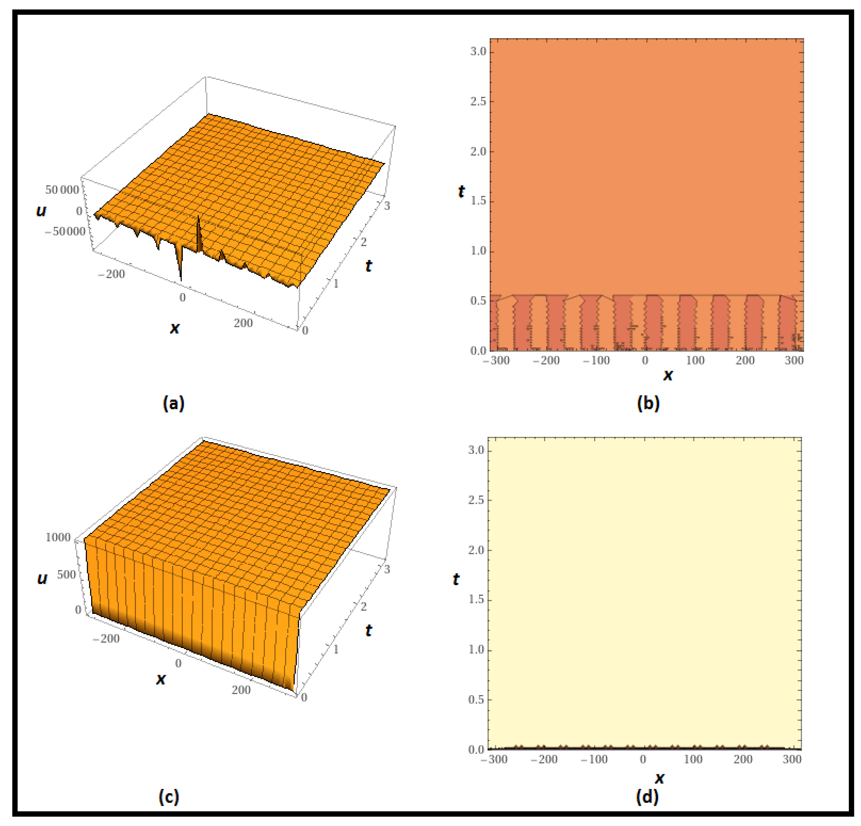
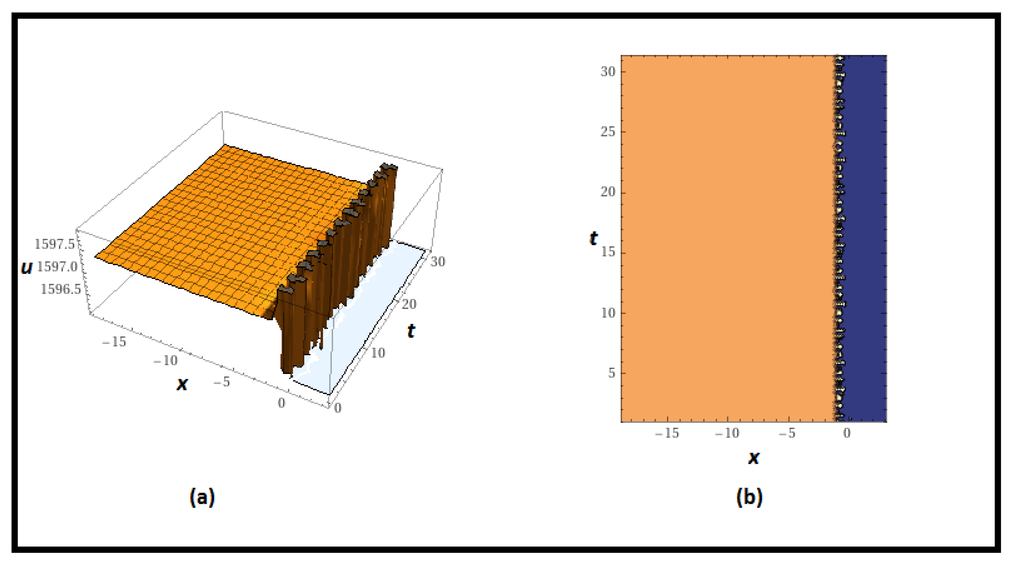
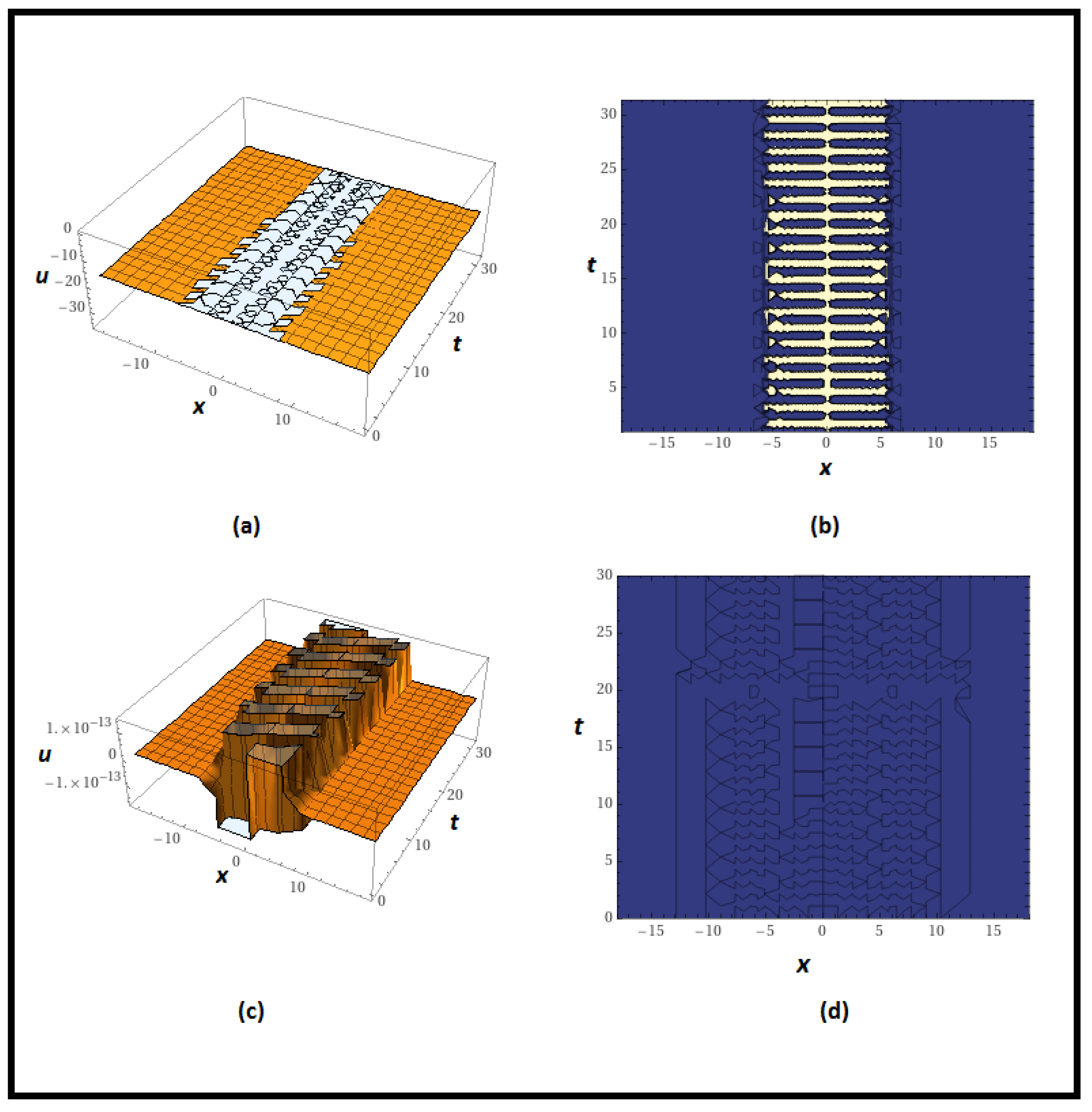
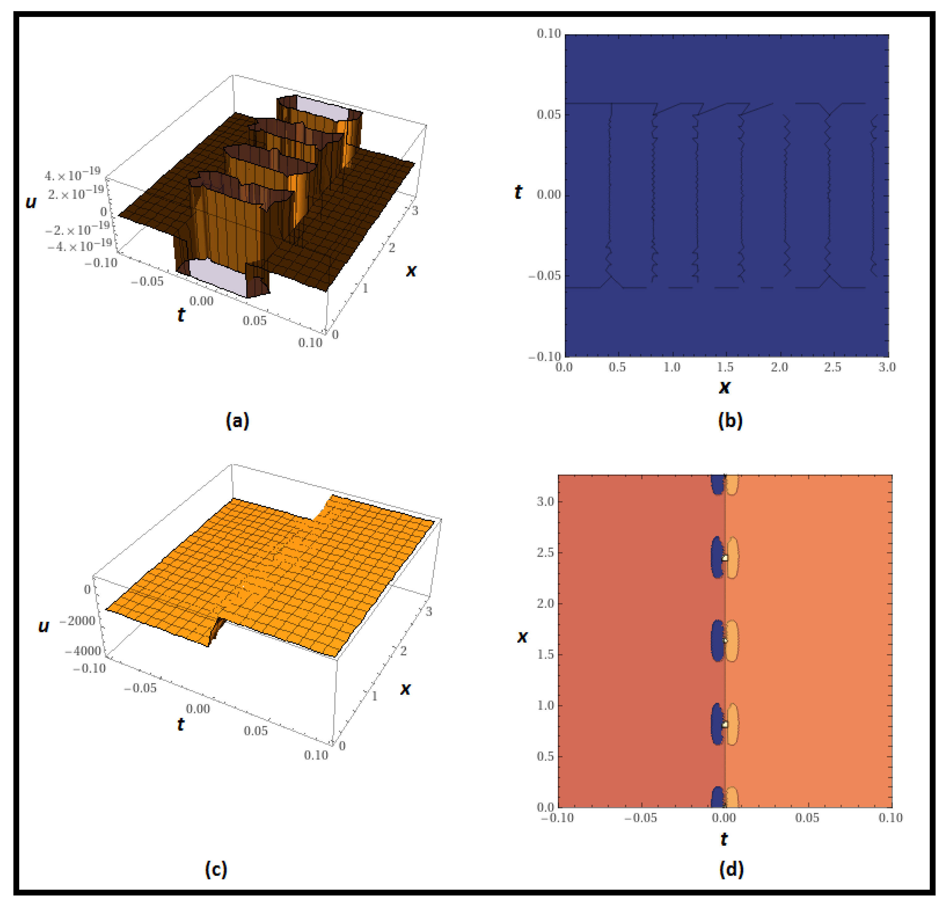
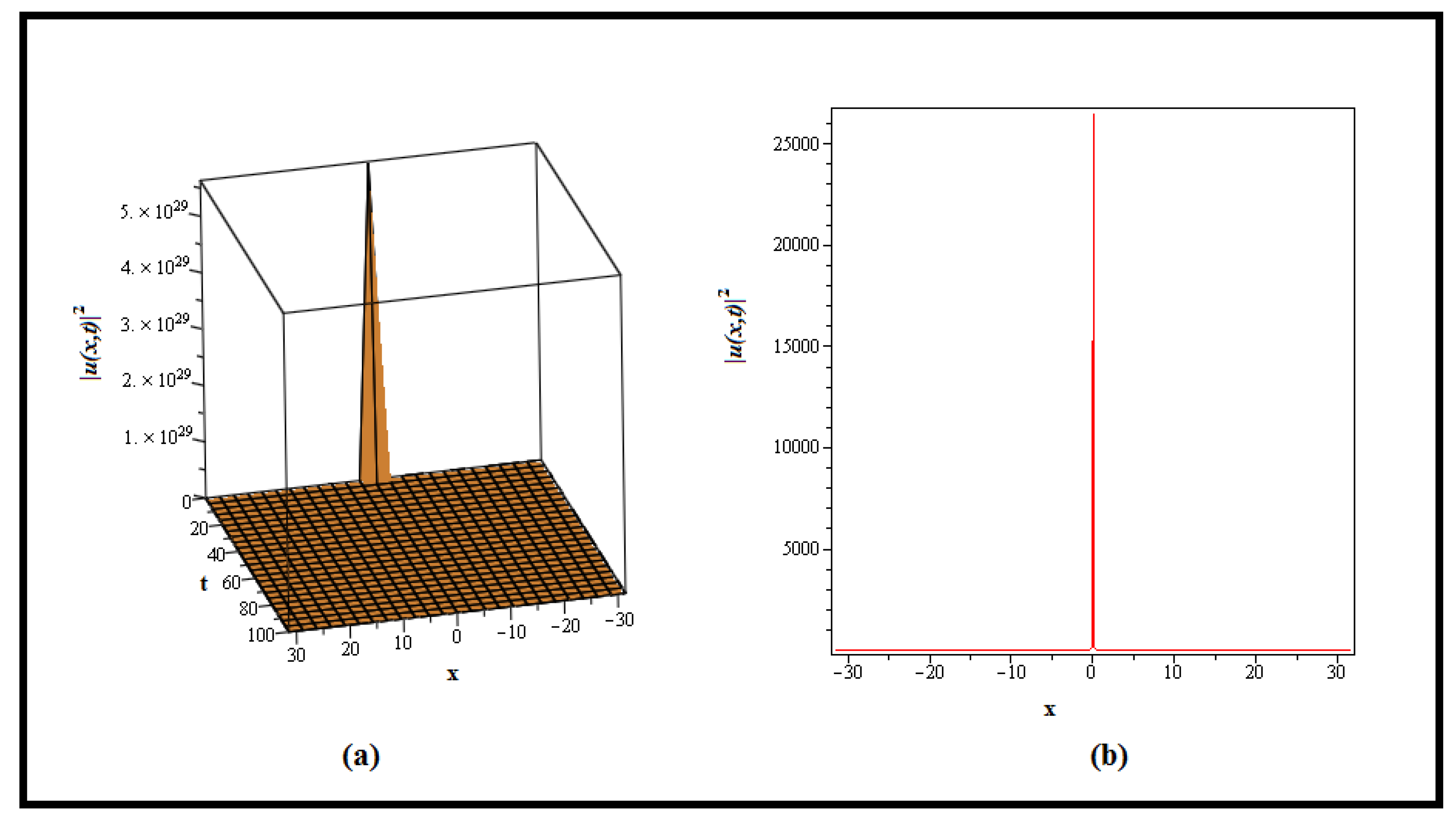
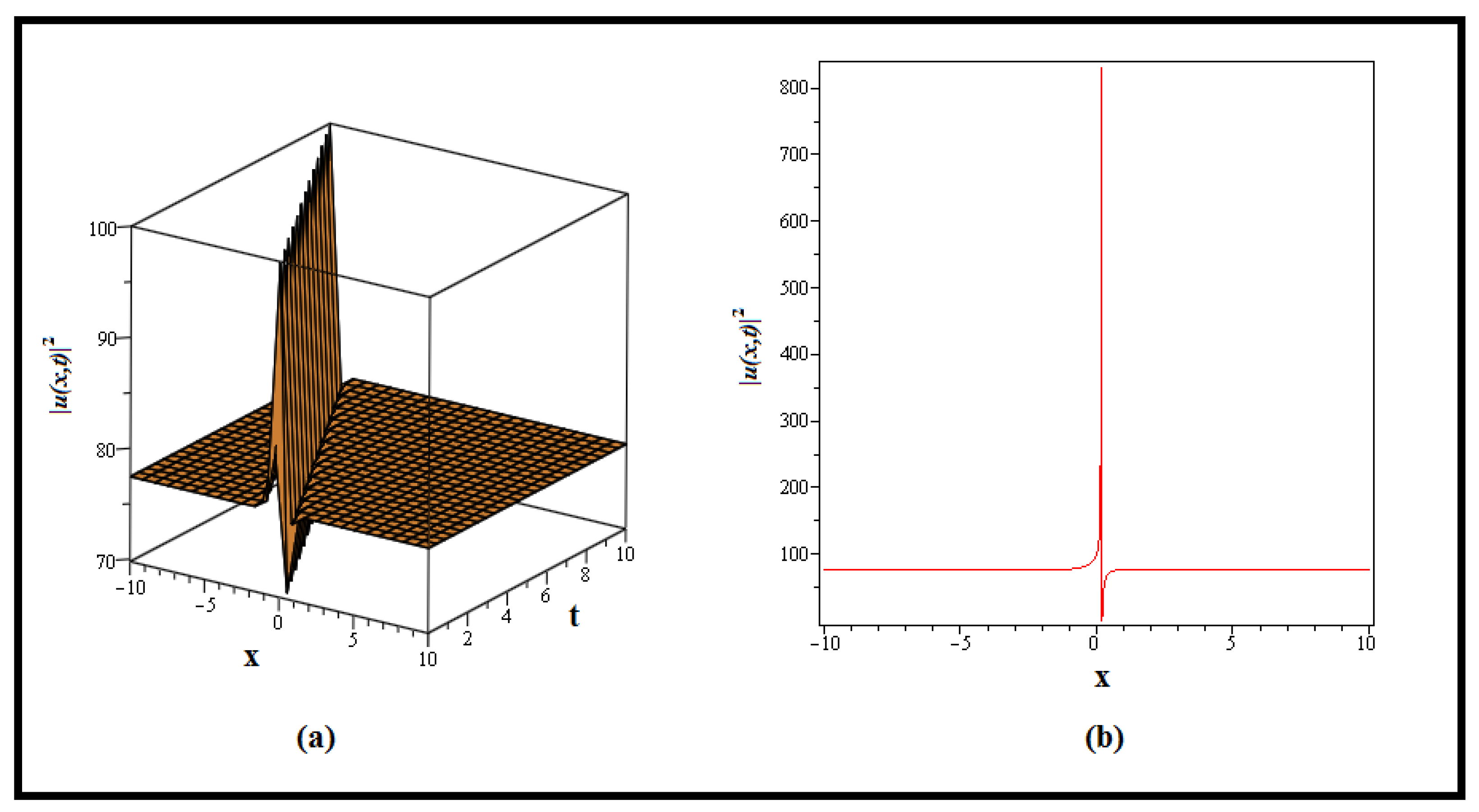
Remark 1.

Overall, Figure 1 shows the solitary kink wave profile, which is a special and distinctive wave form distinguished by a steep bend or abrupt change in direction.

Remark 2.

Overall, Figure 2 shows a lump wave, which is a little bulge or disturbance in a waveform that exhibits a quick rise in amplitude followed by a steady fall to its initial level.

Remark 3.

Figure 3 shows the periodic kink wave profile, which is a special and distinctive wave form distinguished by a steep bend or abrupt change in direction.

Remark 4.

Overall, lone rogue wave, a rare and extreme oceanic occurrence in physics, is depicted in Figure 4. With a noticeably larger amplitude and steeper profile than the other waves, it stands out for its size and unpredictability.

Remark 5.

Overall, a singular kink wave is depicted in Figure 5. Singular kink waves are nonlinear wave system amplitude or phase variations that occur in a variety of scientific environments, including particle physics. They are especially important in theories including scalar fields, such as the Higgs field in the Standard Model, which influences particle mass. To solve unexplained events, extensions such as the “Fractional Coupled Higgs System” include more scalar fields. The mEDAM’s analysis of these waves provides insights into the interaction of new scalar fields with the Higgs field. This research extends particle physics beyond the Standard Model by improving scalar field comprehension in the Higgs region.

Remark 6.

Overall, a lump wave is depicted in Figure 6. A lump wave, also known as a compacton, is a specialized localized solution in nonlinear systems that, unlike other waves, retains a fixed spatial extent while propagating. Nonlinear and dispersive effects cause this behavior. The study of lump waves is relevant in the context of the “Fractional Coupled Higgs System”, an extension of the Standard Model of particle physics. The study of lump waves within this system, which includes various scalar fields in addition to the Higgs field, provides insights on scalar field behavior and interactions. Exploring lump waves contributes to a better understanding of scalar field dynamics and their influence on system behavior, which contributes to the larger objective of grasping extended particle physics models and hypothetical phenomena beyond the standard model.

5. Conclusions

We used mEDAM’s power to construct insightful solitary wave solutions for the fractional coupled Higgs system, adding critical generalized functions to describe its intricate physical processes. We investigated the dynamic behavior of adjustable free parameters and built practical linkages by incorporating them. This study expands our understanding of the system’s features and dynamic patterns, proving mEDAM’s resilience in decoding complicated mathematical models. The relevance of these results extends beyond engineering and scientific areas, promising useful paths for future research into the complicated dynamics of the fractional coupled Higgs system and its associated phenomena.

References

1. Abro, K.A.; Atangana, A. Dual fractional modeling of rate type fluid through non-local differentiation. Numer. Methods Partial Differ. Equ. 2020, 38, 390–405. [Google Scholar] [CrossRef]
2. Metzler, R.; Glöckle, W.G.; Nonnenmacher, T.F. Fractional model equation for anomalous diffusion. Phys. Stat. Mech. Its Appl. 1994, 211, 13–24. [Google Scholar] [CrossRef]
3. Tarasov, V.E.; Zaslavsky, G.M. Fractional dynamics of systems with long-range interaction. Commun. Nonlinear Sci. Numer. Simul. 2006, 11, 885–898. [Google Scholar] [CrossRef]
4. Su, N. Random fractional partial differential equations and solutions for water movement in soils: Theory and applications. Hydrol. Process. 2023, 37, e14844. [Google Scholar] [CrossRef]
5. Che, J.; Guan, Q.; Wang, X. Image denoising based on adaptive fractional partial differential equations. In Proceedings of the 2013 6th International Congress on Image and Signal Processing (CISP), Hangzhou, China, 16–18 December 2013; Volume 1, pp. 288–292. [Google Scholar]
6. Kachhia, K.B.; Prajapati, J.C. Solution of fractional partial differential equation aries in study of heat transfer through diathermanous materials. J. Interdiscip. Math. 2015, 18, 125–132. [Google Scholar] [CrossRef]
7. Zhang, Y. A finite difference method for fractional partial differential equation. Appl. Math. Comput. 2009, 215, 524–529. [Google Scholar] [CrossRef]
8. Ford, N.J.; Xiao, J.; Yan, Y. A finite element method for time fractional partial differential equations. Fract. Calc. Appl. Anal. 2011, 14, 454–474. [Google Scholar] [CrossRef]
9. Lyu, W.; Wang, Z.A. Global classical solutions for a class of reaction-diffusion system with density-suppressed motility. arXiv 2021, arXiv:2102.08042. [Google Scholar] [CrossRef]
10. Li, C.; Chen, A. Numerical methods for fractional partial differential equations. Int. J. Comput. Math. 2018, 95, 1048–1099. [Google Scholar] [CrossRef]
11. Yang, Q.; Liu, F.; Turner, I. Numerical methods for fractional partial differential equations with Riesz space fractional derivatives. Appl. Math. Model. 2010, 34, 200–218. [Google Scholar] [CrossRef]
12. Lin, X.; Liu, Y.; Yu, J.; Yu, R.; Zhang, J.; Wen, H. Stability analysis of three-phase grid-connected inverter under the weak grids with asymmetrical grid impedance by LTP theory in time domain. Int. J. Electr. Power Energy Syst. 2022, 142, 108244. [Google Scholar] [CrossRef]
13. Naeem, M.; Azhar, O.F.; Zidan, A.M.; Nonlaopon, K.; Shah, R. Numerical analysis of fractional-order parabolic equations via Elzaki transform. J. Funct. Spaces 2021, 2021, 3484482. [Google Scholar] [CrossRef]
14. Liu, X.; Shi, T.; Zhou, G.; Liu, M.; Yin, Z.; Yin, L.; Zheng, W. Emotion classification for short texts: An improved multi-label method. Humanit. Soc. Sci. Commun. 2023, 10, 306. [Google Scholar] [CrossRef]
15. Al-Sawalha, M.M.; Ababneh, O.Y.; Shah, R.; Nonlaopon, K. Numerical analysis of fractional-order Whitham-Broer-Kaup equations with non-singular kernel operators. Aims Math. 2023, 8, 2308–2336. [Google Scholar] [CrossRef]
16. Liu, X.; Zhou, G.; Kong, M.; Yin, Z.; Li, X.; Yin, L.; Zheng, W. Developing Multi-Labelled Corpus of Twitter Short Texts: A Semi-Automatic Method. Systems 2023, 11, 390. [Google Scholar] [CrossRef]
17. Chen, D.; Wang, Q.; Li, Y.; Li, Y.; Zhou, H.; Fan, Y. A general linear free energy relationship for predicting partition coefficients of neutral organic compounds. Chemosphere 2020, 247, 125869. [Google Scholar] [CrossRef]
18. Elagan, S.K.; Sayed, M.; Higazy, M. An analytical study on fractional partial differential equations by Laplace transform operator method. Int. J. Appl. Eng. Res. 2018, 13, 545–549. [Google Scholar]
19. Mahor, T.C.; Mishra, R.; Jain, R. Analytical solutions of linear fractional partial differential equations using fractional Fourier transform. J. Comput. Appl. Math. 2021, 385, 113202. [Google Scholar] [CrossRef]
20. Thabet, H.; Kendre, S. New modification of Adomian decomposition method for solving a system of nonlinear fractional partial differential equations. Int. J. Adv. Appl. Math. Mech. 2019, 6, 1–13. [Google Scholar]
21. Duran, S. Exact solutions for time-fractional Ramani and Jimbo—Miwa equations by direct algebraic method. Adv. Sci. Eng. Med. 2020, 12, 982–988. [Google Scholar] [CrossRef]
22. Momani, S.; Odibat, Z. Homotopy perturbation method for nonlinear partial differential equations of fractional order. Phys. Lett. A 2007, 365, 345–350. [Google Scholar] [CrossRef]
23. Odibat, Z.; Momani, S. The variational iteration method: An efficient scheme for handling fractional partial differential equations in fluid mechanics. Comput. Math. Appl. 2009, 58, 2199–2208. [Google Scholar] [CrossRef]
24. Mirhosseini-Alizamini, S.M.; Rezazadeh, H.; Eslami, M.; Mirzazadeh, M.; Korkmaz, A. New extended direct algebraic method for the Tzitzica type evolution equations arising in nonlinear optics. Comput. Methods Differ. Equ. 2020, 8, 28–53. [Google Scholar]
25. Yasmin, H.; Aljahdaly, N.H.; Saeed, A.M.; Shah, R. Investigating Symmetric Soliton Solutions for the Fractional Coupled Konno–Onno System Using Improved Versions of a Novel Analytical Technique. Mathematics 2023, 11, 2686. [Google Scholar] [CrossRef]
26. Yasmin, H.; Aljahdaly, N.H.; Saeed, A.M.; Shah, R. Probing Families of Optical Soliton Solutions in Fractional Perturbed Radhakrishnan–Kundu–Lakshmanan Model with Improved Versions of Extended Direct Algebraic Method. Fractal Fract. 2023, 7, 512. [Google Scholar] [CrossRef]
27. Rezazadeh, H.; Mirhosseini-Alizamini, S.M.; Neirameh, A.; Souleymanou, A.; Korkmaz, A.; Bekir, A. Fractional Sine–Gordon equation approach to the coupled higgs system defined in time-fractional form. Iran. J. Sci. Technol. Trans. A Sci. 2019, 43, 2965–2973. [Google Scholar] [CrossRef]
28. Jabbari, A.; Kheiri, H.; Bekir, A. Exact solutions of the coupled Higgs equation and the Maccari system using He’s semi-inverse method and (G’/G)-expansion method. Comput. Math. Appl. 2011, 62, 2177–2186. [Google Scholar] [CrossRef]
29. Atas, S.S.; Ali, K.K.; Sulaiman, T.A.; Bulut, H. Invariant optical soliton solutions to the Coupled-Higgs equation. Opt. Quantum Electron. 2022, 54, 754. [Google Scholar] [CrossRef]
30. Seadawy, A.R.; Lu, D.; Khater, M.M. Bifurcations of traveling wave solutions for Dodd–Bullough–Mikhailov equation and coupled Higgs equation and their applications. Chin. J. Phys. 2017, 55, 1310–1318. [Google Scholar] [CrossRef]
31. Mu, G.; Qin, Z. Rogue waves for the coupled Schrödinger–Boussinesq equation and the coupled Higgs equation. J. Phys. Soc. Jpn. 2012, 81, 084001. [Google Scholar] [CrossRef]
32. Sikora, B. Remarks on the Caputo fractional derivative. MINUT 2023, 5, 76–84. [Google Scholar]
33. Khan, H.; Barak, S.; Kumam, P.; Arif, M. Analytical Solutions of Fractional Klein-Gordon and Gas Dynamics Equations, via the (G/G)-Expansion Method. Symmetry 2019, 11, 566. [Google Scholar] [CrossRef]
Figure 1. Graph of (28) in which (a,b) present 3D and contour plots of real part respectively while (c,d) present 3D and contour plots of imaginary part respectively for  a = 3 , b = 1 , c = 5 , A = e a 1 = 1000 , b 1 = 0 , γ = δ = 1 .
Fractalfract 07 00653 g001
Figure 2. Graph of (46) in which (a,b) present 3D and contour plots of real part respectively while (c,d) and present 3D and contour plots of imaginary part respectively for  a = 3 , b = 0 , c = 5 , A = e a 1 = 1000 , b 1 = 0 , γ = δ = 1 .
Fractalfract 07 00653 g002
Figure 3. Graph of the real part of (136) in which (a,b) present 3D and contour plots of real part respectively for  a = 3 , b = 10 , c = 5 , A = 2 , a 1 = 1000 , b 1 = 0 , γ = δ = 1 .
Fractalfract 07 00653 g003
Figure 4. Graph of (204) in which (a,b) present 3D and contour plots of real part respectively while (c,d) present 3D and contour plots of imaginary part respectively for  a = 3 , b = 0 , c = 3 , A = e a 1 = 1000 , b 1 = 10 , 000 , γ = δ = 1 .
Fractalfract 07 00653 g004
Figure 5. Depicts graph of the squared norm of (44). The 3D graph in (a) is plotted for  a = 3 b = 10 , c = 1 , A = e , a 1 = b 1 = 25 , γ = δ = 1 while the 2D graph in (b) is drawn for  t = 0 and the similar values of involved parameters.
Fractalfract 07 00653 g005
Figure 6. Depicts graph of the squared norm of (62). The 3D graph in (a) is plotted for  a = 2 b = 0 , c = 1 , A = e , a 1 = 0 , b 1 = 0 , γ = δ = 1 while the 2D graph in (b) is drawn for  t = 0 and the similar values of involved parameters.
Fractalfract 07 00653 g006
Disclaimer/Publisher’s Note: The statements, opinions and data contained in all publications are solely those of the individual author(s) and contributor(s) and not of MDPI and/or the editor(s). MDPI and/or the editor(s) disclaim responsibility for any injury to people or property resulting from any ideas, methods, instructions or products referred to in the content.