Computational Study for Fiber Bragg Gratings with Dispersive Reflectivity Using Fractional Derivative

Abstract

In this paper, the new representations of optical wave solutions to fiber Bragg gratings with cubic–quartic dispersive reflectivity having the Kerr law of nonlinear refractive index structure are retrieved with high accuracy. The residual power series technique is used to derive power series solutions to this model. The fractional derivative is taken in Caputo’s sense. The residual power series technique (RPST) provides the approximate solutions in truncated series form for specified initial conditions. By using three test applications, the efficiency and validity of the employed technique are demonstrated. By considering the suitable values of parameters, the power series solutions are illustrated by sketching 2D, 3D, and contour profiles. The analysis of the obtained results reveals that the RPST is a significant addition to exploring the dynamics of sustainable and smooth optical wave propagation across long distances through optical fibers.

1. Introduction

Over the last few decades, the investigation of optical wave propagation has caught the attention of different scientists in applied mathematics. Many significant developments have been made in the field of nonlinear optics [1,2,3,4,5]. In the realm of nonlinear optics, it is widely known that the propagation of an optical pulse in nonlinear media, including Kerr law and non-Kerr law, may be represented by the nonlinear Schrödinger equation [6]. The Kerr law of nonlinearity arises when a light wave in an optical fiber experiences nonlinear responses due to nonharmonic motion of electrons caused by an external electric field [7,8,9]. Low chromatic dispersion is one of the fundamental issues with soliton transmission over intercontinental distances. To manage and lessen this effect, a number of strategies and approaches have been applied. The project was then successfully completed by adding gratings to optical fibers [10,11,12].

One of the most inventive technologies applied to nonlinear optics is fiber Bragg grating (FBG) [13]. FBG technology has been embraced by the field of fiber optics since its discovery. Presently, most fiber optic sensor systems use FBG technology. Due to the inherent benefits of FBGs, including their compact size, quick reaction, dispersed sensing, and immunity to the electromagnetic field, FBG-based sensing has attracted a lot of research interest [14]. Measurements of numerous physical parameters, including temperature, pressure, and strain are frequently performed using FBG technology [15]. For a wide range of applications, FBGs are also useful in signal shaping as well as filtering components [16].

Occasionally, another difficulty comes when the chromatic dispersion is gradually depleted, and hence, there is an unstable balance between the chromatic dispersion and the nonlinearity, being followed by a possible pulse collapse. To overcome this difficulty, the chromatic dispersion is replaced by a combination of third-order and fourth-order dispersions.

Optical waves in FBGs with different nonlinear refractive indices, where the chromatic dispersion is replaced by the third- and fourth-order dispersions together with the dispersive reflectivity have been retrieved analytically in the earlier studies. For example, Wang et al. [17] investigated this model by implementing the trial equation approach to retrieve cubic–quartic optical solitons in FBGs. Yildirim et al. [18] retrieved the soliton solutions of this model with the sine-Gordon equation method. Malik et al. [19] investigated the nonlinear Schrödinger equation, which considered the cubic–quartic form of nonlinear refractive index with parabolic law of nonlinearity by Lie symmetry. Arnous et al. [20] derived the optical solitons in FBGs with cubic–quartic dispersive reflectivity with the aid of enhanced Kudryashov’s technique. Zayed et al. [21] used the auxiliary equation approach to explore solitons in FBGs with cubic–quartic dispersive reflectivity having the Kerr law of nonlinear refractive index.

In this paper, we consider a model in FBGs with cubic–quartic dispersive reflectivity having a Kerr nonlinear refractive index and Caputo’s time-fractional derivative of order $\varrho$ ($0<\varrho \le 1$). The mathematical form of the considered model is expressed as

$$\begin{array}{cc}\hfill \iota D_t^{\varrho }n+\iota a_1{o}_{\varpi \varpi \varpi }+b_1{o}_{\varpi \varpi \varpi \varpi }+(c_1{\left|n\right|}^2+d_1{\left|o\right|}^2)n+\iota {\alpha }_1{n}_{\varpi }+{\beta }_{1}o=0,& \\ \hfill \iota D_t^{\varrho }o+\iota a_2{n}_{\varpi \varpi \varpi }+b_2{n}_{\varpi \varpi \varpi \varpi }+(c_2{\left|n\right|}^2+d_2{\left|n\right|}^2)o+\iota {\alpha }_2{o}_{\varpi }+{\beta }_{2}n=0,\end{array}$$

(1)

where $n(\varpi ,t)$ and $o(\varpi ,t)$ denote wave profiles, and t and $\varpi$ denote the time in dimensionless form and the non-dimensional distance, respectively. The coefficients $a_j,b_j,{\alpha }_j,c_j,d_j$ and ${\beta }_j$ correspond to third-order dispersion, fourth-order dispersion, intermodal dispersion, self-phase modulation, cross-phase modulation, and detuning parameters, respectively. The exact solution of this model at $\varrho =1$ is reported by Ming-Yue-Wang et al. [17].

The primary goal of this work is to present the optical wave solutions and their graphical observations for the considered model in FBGs with Caputo’s time-fractional derivative using the residual power series technique (RPST). The obtained results are novel, and the proposed technique is utilized for the first time to study the considered fractional model in this work.

The discipline of fractional calculus has seen tremendous advancements in study at the intersection of probability, chaos, differential equations, and mathematical physics [22,23,24,25,26]. The nonlocal property of fractional differential equations (FDEs) is a significant advantage of employing them in various mathematical modeling. Retrieving the analytical solutions for FDEs is sometimes difficult to achieve due to the computational complexities of fractional operators. In this respect, numerous methods have been constructed and motivated to investigate the approximate solution for FDEs, among which are the Sinc-collocation method [27], the predictor–corrector compact difference scheme [28], the variational iteration method [29], the homotopy analysis technique [30], the homotopy asymptotic method [31], the homotopy perturbation scheme [32], the differential transform method [33], the linearly compact scheme [34], the Adomian decomposition method [35] etc.

One of the most efficient techniques for exploring approximate analytic solutions for linear and nonlinear FDEs is the residual power series technique (RPST) [36,37,38,39,40]. The RPST was introduced by the Jordan mathematician Abu Arqub [41]. The RPST has been successfully used to construct the approximate analytic solutions of FDEs without implementing linearization, perturbation, or discretization techniques, showing the reliability and simplicity of this technique. This proposed technique has been successfully applied to investigate the solutions of time-fractional Whitham–Broer–Kaup equations [42], Black–Scholes European option pricing equations [43], the KdV equation [44], the nonlinear Schrödinger equation [45], the Biswas–Milovic equation [46], the Caudrey–Dodd–Gibbon–Sawada–Kotera equation [47], etc. The suggested technique is a reliable, practical, and astonishingly effective tool for examining the approximate solutions of many types of real-life nonlinear models.

The RPST has several advantages. It is well-known for its accuracy and simplicity to obtain the desired results. It does not require variable discretization, and there is no requirement for huge computer memory or time to reach the solutions. Its nature is global regarding the approximate analytical solutions, which makes it useful to investigate various mathematical, engineering, and physical problems. Being analytic expressions, the results obtained through the RPST can be further explored with derivative calculations.

The arrangement of this paper is given in the following manner. Some preliminaries of fractional calculus and the RPST are presented in Section 2. A description of the fundamental steps of the proposed method and the construction of a solution to the suggested problem is illustrated in Section 3. Graphical findings for different applications are exhibited in Section 4. The conclusion is presented in the last section.

2. Preliminaries

This section introduces the fundamental properties of fractional calculus theory, allowing us to follow the solutions of a coupled nonlinear Schrödinger equation for the Kerr law of nonlinear refractive index in FBGs.

The Caputo technique is chosen in this study because it is appropriate for real-world physical problems, and it specifies integer-order initial conditions for FDEs.

Definition 1 

([22]). Caputo’s time-fractional derivative of order ϱ of $\delta (\varpi ,t)$ is defined as

$$D_t^{\varrho }\delta (\varpi ,t)=\left\{\begin{array}{c}\frac{1}{\Gamma (\zeta -\varrho )}{\int }_0^t{(t-\psi )}^{\zeta -\varrho -1}\frac{{\partial }^{\zeta }\delta (\varpi ,\psi )}{\partial {\psi }^{\zeta }}d\psi ,0\le \zeta -1<\varrho <\zeta ,t>\psi >s\ge 0,\varpi \in I,\hfill \\ \\ \frac{{\partial }^{\zeta }\delta (\varpi ,t)}{\partial t^{\zeta }},\varrho =\zeta \in N.\hfill \end{array}\right.$$

Theorem 1 

([22]). If $\zeta -1<\varrho \le \zeta ,$$\zeta \in N$, then

(a) 

$D_t^{\varrho }{I}_t^{\varrho }\delta (\varpi ,t)=\delta (\varpi ,t),$

(b) 

$I_t^{\varrho }{D}_t^{\varrho }\delta (\varpi ,t)=\delta (\varpi ,t)-{\sum }_{i=0}^{n-1}\frac{{\partial }^i\delta (\varpi ,s^{+})}{\partial t^i}\frac{t^i}{i!}.$

Lemma 1 

([22]). If $f(\varpi )$ is a continuous function and $\varrho ,\vartheta >0$, then the following result holds:

$$I_a^{\varrho }{I}_a^{\vartheta }f(\varpi )=I_a^{\varrho }{I}_a^{\vartheta }f(\varpi )=I_a^{\varrho +\vartheta }f(\varpi ).$$

(2)

Other basic properties of fractional-order derivatives are shown in [22,23,24]. Some results from [48] that are important for the RPST are as follows:

Definition 2. 

A power series of the following form

$$\sum _{k=0}^{\infty }{e}_k{(t-t_0)}^{k\varrho }=e_0+e_1{(t-t_0)}^{\varrho }+e_2{(t-t_0)}^{2\varrho }+\dots ,0\le \zeta -1<\varrho \le \zeta ,t\ge t_0,$$

(3)

is a fractional power series about $t=t_0$.

Definition 3. 

A multiple fractional power series about $t=t_0$, for $0\le \zeta -1<\varrho \le \zeta$ is defined as follows:

$$\sum _{k=0}^{\infty }\widetilde{{\delta }_k}(\varpi ){(t-t_0)}^{k\varrho }=\widetilde{{\delta }_0}(\varpi )+\widetilde{{\delta }_1}(\varpi ){(t-t_0)}^{\varrho }+\widetilde{{\delta }_2}(\varpi ){(t-t_0)}^{2\varrho }+\dots ,t\ge t_0,$$

(4)

where the coefficients of the series are ${\tilde{\delta }}_k$ and are functions of ϖ.

Theorem 2. 

Assume that δ has a fractional power series representation of the form at $t=t_0$,

$$\delta (t)=\sum _{k=0}^{\infty }{e}_k{(t-t_0)}^{k\varrho },0\le \zeta -1<\varrho \le \zeta ,t_0\le t<t_0+R.$$

(5)

If $D^{k\varrho }\delta (t)$ are continuous on $(t_0,t_0+R),k=0,1,2,\dots ,$ then the coefficients “$e_k$" appearing in Equation (5) can be determined as

$$e_k=\frac{D^{k\varrho }\delta (t_0)}{\Gamma (k\varrho +1)},$$

where R is considered as the series’s radius of convergence.

Other results related to the RPST can be found in [37,48,49].

3. RPST to FBGs for Cubic-Quartic Dispersive Reflectivity with Time-Fractional Derivative

Consider a coupled nonlinear Schrödinger equation with the cubic–quartic dispersive reflectivity having the Kerr law of nonlinear refractive index as

$$\begin{array}{cc}\hfill \iota D_t^{\varrho }n+\iota a_1{o}_{\varpi \varpi \varpi }+b_1{o}_{\varpi \varpi \varpi \varpi }+(c_1{\left|n\right|}^2+d_1{\left|o\right|}^2)n+\iota {\alpha }_1{n}_{\varpi }+{\beta }_{1}o=0,& \\ \hfill \iota D_t^{\varrho }o+\iota a_2{n}_{\varpi \varpi \varpi }+b_2{n}_{\varpi \varpi \varpi \varpi }+(c_2{\left|n\right|}^2+d_2{\left|n\right|}^2)o+\iota {\alpha }_2{o}_{\varpi }+{\beta }_{2}n=0,\end{array}$$

(6)

subject to the initial conditions

$$\begin{array}{cc}\hfill n(\varpi ,0)=\tilde{q}(\varpi ),& \\ \hfill o(\varpi ,0)=\tilde{r}(\varpi ),\end{array}$$

(7)

where $D_t^{\varrho }$ represents Caputo’s time-fractional derivative of order $\varrho$. The fundamental goal of this work is to develop the solution for Equations (6) and (7) by its power series expansion among its truncated residual function.

For the construction of power series solutions of Equations (6) and (7), let

$$\begin{array}{cc}\hfill n(\varpi ,t)=p(\varpi ,t)+\iota s(\varpi ,t),& \\ \hfill o(\varpi ,t)=u(\varpi ,t)+\iota w(\varpi ,t),\end{array}$$

(8)

where $n(\varpi ,0)=p(\varpi ,0)+\iota s(\varpi ,0)$, and $o(\varpi ,0)=u(\varpi ,0)+\iota w(\varpi ,0)$. The following system can be obtained using the above equations in (6) and (7) as

$$\begin{array}{cc}\hfill D_t^{\varrho }s+a_1{w}_{\varpi \varpi \varpi }-b_1{u}_{\varpi \varpi \varpi \varpi }-c_{1}p(p^2+s^2)-d_{1}p(u^2+w^2)+{\alpha }_1{s}_{\varpi }-{\beta }_{1}u=0,& \\ \hfill D_t^{\varrho }p+a_1{u}_{\varpi \varpi \varpi }+b_1{w}_{\varpi \varpi \varpi \varpi }+c_{1}s(p^2+s^2)+d_{1}s(u^2+w^2)+{\alpha }_1{p}_{\varpi }+{\beta }_{1}w=0,& \\ \hfill D_t^{\varrho }w+a_2{s}_{\varpi \varpi \varpi }-b_2{p}_{\varpi \varpi \varpi \varpi }-c_{2}u(u^2+w^2)-d_{2}u(p^2+s^2)+{\alpha }_2{w}_{\varpi }-{\beta }_{2}p=0,& \\ \hfill D_t^{\varrho }u+a_2{p}_{\varpi \varpi \varpi }+b_2{s}_{\varpi \varpi \varpi \varpi }+c_{2}w(u^2+w^2)+d_{2}w(p^2+s^2)+{\alpha }_2{u}_{\varpi }+{\beta }_{2}s=0,\end{array}$$

(9)

with initial conditions

$$\begin{array}{cc}\hfill p(\varpi ,0)={\sigma }_1(\varpi ),& \\ \hfill s(\varpi ,0)={\sigma }_2(\varpi ),& \\ \hfill u(\varpi ,0)={\xi }_1(\varpi ),& \\ \hfill w(\varpi ,0)={\xi }_2(\varpi ),\end{array}$$

(10)

where $\tilde{q}(\varpi )={\sigma }_1(\varpi )+\iota {\sigma }_2(\varpi )$, and $\tilde{r}(\varpi )={\xi }_1(\varpi )+\iota {\xi }_2(\varpi ).$

3.1. General Procedure of the RPST

The following are the primary steps for the recommended process.

• Step A. Assume the fractional power series solutions of above system regarding the initial point $(t=0)$ as

  $$\begin{array}{cc}\hfill & p(\varpi ,t)=\sum _{k=0}^{\infty }{g}_k(\varpi )\frac{t^{k\varrho }}{\Gamma (k\varrho +1)},\hfill \\ \hfill & s(\varpi ,t)=\sum _{k=0}^{\infty }{f}_k(\varpi )\frac{t^{k\varrho }}{\Gamma (k\varrho +1)},\hfill \\ \hfill & u(\varpi ,t)=\sum _{k=0}^{\infty }{l}_k(\varpi )\frac{t^{k\varrho }}{\Gamma (k\varrho +1)},\hfill \\ \hfill & w(\varpi ,t)=\sum _{k=0}^{\infty }{m}_k(\varpi )\frac{t^{k\varrho }}{\Gamma (k\varrho +1)}.\hfill \end{array}$$

  (11)

For the numerical values of fractional power series solutions for the system of equations with initial conditions, take the $z-th$ truncated series of $p(\varpi ,t),s(\varpi ,t),u(\varpi ,t)$, and $w(\varpi ,t)$ as $p_z(\varpi ,t),s_z(\varpi ,t),u_z(\varpi ,t)$, and $w_z(\varpi ,t)$, respectively, i.e.,

$$\begin{array}{cc}\hfill & p_z(\varpi ,t)=\sum _{k=0}^z{g}_k(\varpi )\frac{t^{k\varrho }}{\Gamma (k\varrho +1)},\hfill \\ \hfill & s_z(\varpi ,t)=\sum _{k=0}^z{f}_k(\varpi )\frac{t^{k\varrho }}{\Gamma (k\varrho +1)},\hfill \\ \hfill & u_z(\varpi ,t)=\sum _{k=0}^z{l}_k(\varpi )\frac{t^{k\varrho }}{\Gamma (k\varrho +1)},\hfill \\ \hfill & w_z(\varpi ,t)=\sum _{k=0}^z{m}_k(\varpi )\frac{t^{k\varrho }}{\Gamma (k\varrho +1)}.\hfill \end{array}$$

(12)

Using the initial conditions, the $0-th$ fractional power series solutions can be obtained as

$$\begin{array}{cc}\hfill p_0(\varpi ,t)=g_0(\varpi )={\sigma }_1(\varpi ),& \\ \hfill s_0(\varpi ,t)=f_0(\varpi )={\sigma }_2(\varpi ),& \\ \hfill u_0(\varpi ,t)=l_0(\varpi )={\xi }_1(\varpi ),& \\ \hfill w_0(\varpi ,t)=m_0(\varpi )={\xi }_2(\varpi ).\end{array}$$

(13)

The system of Equations (12) can be rewritten as

$$\begin{array}{cc}\hfill p_z(\varpi ,t)={\sigma }_1(\varpi )+\sum _{k=1}^z{g}_k(\varpi )\frac{t^{k\varrho }}{\Gamma (k\varrho +1)},& \\ \hfill s_z(\varpi ,t)={\sigma }_2(\varpi )+\sum _{k=1}^z{f}_k(\varpi )\frac{t^{k\varrho }}{\Gamma (k\varrho +1)},& \\ \hfill u_z(\varpi ,t)={\xi }_1(\varpi )+\sum _{k=1}^z{l}_k(\varpi )\frac{t^{k\varrho }}{\Gamma (k\varrho +1)},& \\ \hfill w_z(\varpi ,t)={\xi }_2(\varpi )+\sum _{k=1}^z{m}_k(\varpi )\frac{t^{k\varrho }}{\Gamma (k\varrho +1)}.\end{array}$$

(14)

The required expressions for $z-th$ fractional power series solutions will be obtained by varying $k=1,2,3,\cdots ,z$ in $p(\varpi ,t),s(\varpi ,t),u(\varpi ,t)$, and $w(\varpi ,t)$.

• Step B. For Equations (9) and (10), the residual functions will be constructed. This construction will be made in the following manner as

  $$\begin{array}{cc}\hfill Re{s}_p(\varpi ,t)=\frac{{\partial }^{\varrho }s}{\partial t^{\varrho }}+a_1\frac{{\partial }^{3}w}{\partial {\varpi }^3}-b_1\frac{{\partial }^{4}u}{\partial {\varpi }^4}-c_{1}p(p^2+s^2)-d_{1}p(u^2+w^2)+{\alpha }_1\frac{\partial s}{\partial \varpi }-{\beta }_{1}u,& \\ \hfill Re{s}_s(\varpi ,t)=\frac{{\partial }^{\varrho }p}{\partial t^{\varrho }}+a_1\frac{{\partial }^{3}u}{\partial {\varpi }^3}+b_1\frac{{\partial }^{4}w}{\partial {\varpi }^4}+c_{1}s(p^2+s^2)+d_{1}s(u^2+w^2)+{\alpha }_1\frac{\partial p}{\partial \varpi }+{\beta }_{1}w,& \\ \hfill Re{s}_u(\varpi ,t)=\frac{{\partial }^{\varrho }w}{\partial t^{\varrho }}+a_2\frac{{\partial }^{3}s}{\partial {\varpi }^3}-b_2\frac{{\partial }^{4}p}{\partial {\varpi }^4}-c_{2}u(u^2+w^2)-d_{2}p(p^2+s^2)+{\alpha }_2\frac{\partial w}{\partial \varpi }-{\beta }_{2}p,& \\ \hfill Re{s}_w(\varpi ,t)=\frac{{\partial }^{\varrho }u}{\partial t^{\varrho }}+a_2\frac{{\partial }^{3}p}{\partial {\varpi }^3}+b_2\frac{{\partial }^{4}s}{\partial {\varpi }^4}+c_{2}w(u^2+w^2)+d_{2}w(p^2+s^2)+{\alpha }_2\frac{\partial u}{\partial \varpi }+{\beta }_{2}s.\end{array}$$

  (15)

Taking $p_z=p_z(\varpi ,t),s_z=s_z(\varpi ,t),u_z=u_z(\varpi ,t)$, and $w_z=w_z(\varpi ,t)$, then the $z-th$ residual functions $z=1,2,3,\cdots$ can be defined as

$$\begin{array}{c}\hfill Re{s}_{p,z}(\varpi ,t)=\frac{{\partial }_z^{\varrho }s}{\partial t^{\varrho }}+a_1\frac{{\partial }^3{w}_z}{\partial {\varpi }^3}-b_1\frac{{\partial }^4{u}_z}{\partial {\varpi }^4}-c_1{p}_z(p_z^2+s_z^2)-d_1{p}_z(u_z^2+w_z^2)+{\alpha }_1\frac{\partial s_z}{\partial \varpi }-{\beta }_1{u}_z,\end{array}$$

$$\begin{array}{c}\hfill Re{s}_{s,z}(\varpi ,t)=\frac{{\partial }^{\varrho }{p}_z}{\partial t^{\varrho }}+a_1\frac{{\partial }^3{u}_z}{\partial {\varpi }^3}+b_1\frac{{\partial }^4{w}_z}{\partial {\varpi }^4}+c_1{s}_z(p_z^2+s_z^2)+d_1{s}_z(u_z^2+w_z^2)+{\alpha }_1\frac{\partial p_z}{\partial \varpi }+{\beta }_1{w}_z,\end{array}$$

$$\begin{array}{c}\hfill Re{s}_{u,z}(\varpi ,t)=\frac{{\partial }^{\varrho }{w}_z}{\partial t^{\varrho }}+a_2\frac{{\partial }^3{s}_z}{\partial {\varpi }^3}-b_2\frac{{\partial }^4{p}_z}{\partial {\varpi }^4}-c_2{u}_z(u_z^2+w_z^2)-d_2{p}_z(p_z^2+s_z^2)+{\alpha }_2\frac{\partial w_z}{\partial \varpi }-{\beta }_2{p}_z,\end{array}$$

$$\begin{array}{c}\hfill Re{s}_{w,z}(\varpi ,t)=\frac{{\partial }^{\varrho }{u}_z}{\partial t^{\varrho }}+a_2\frac{{\partial }^3{p}_z}{\partial {\varpi }^3}+b_2\frac{{\partial }^4{s}_z}{\partial {\varpi }^4}+c_2{w}_z(u_z^2+w_z^2)+d_2{w}_z(p_z^2+s_z^2)+{\alpha }_2\frac{\partial u_z}{\partial \varpi }+{\beta }_2{s}_z.\end{array}$$

(16)

Some important results of $Re{s}_p(\varpi ,t),Re{s}_s(\varpi ,t),Re{s}_u(\varpi ,t)$, and $Re{s}_w(\varpi ,t)$ that are useful for the residual power series solutions for $i=1,2,\cdots ,z$ are stated below:

• $Re{s}_p(\varpi ,t)=0,Re{s}_s(\varpi ,t)=0,Re{s}_u(\varpi ,t)=0,Re{s}_w(\varpi ,t)=0$
• $\underset{z\to \infty }{lim}Re{s}_{p,z}(\varpi ,t)=Re{s}_p(\varpi ,t),\underset{z\to \infty }{lim}Re{s}_{s,z}(\varpi ,t)=Re{s}_s(\varpi ,t)$,
  $\underset{z\to \infty }{lim}Re{s}_{u,z}(\varpi ,t)=Re{s}_u(\varpi ,t),\underset{z\to \infty }{lim}Re{s}_{w,z}(\varpi ,t)=Re{s}_w(\varpi ,t)$ for each $\varpi \in I$ and $t=0$,
• $D^{i\varrho }Re{s}_p(\varpi ,0)=D^{i\varrho }Re{s}_{p,z}(\varpi ,0)=0,$
  $D^{i\varrho }Re{s}_s(\varpi ,0)=D^{i\varrho }Re{s}_{s,z}(\varpi ,0)=0,$
  $D^{i\varrho }Re{s}_u(\varpi ,0)=D^{i\varrho }Re{s}_{u,z}(\varpi ,0)=0,$
  $D^{i\varrho }Re{s}_w(\varpi ,0)=D^{i\varrho }Re{s}_{w,z}(\varpi ,0)=0.$

• Step C. Substituting $p_z(\varpi ,t),s_z(\varpi ,t),u_z(\varpi ,t)$, and $w_z(\varpi ,t)$ into (16) and calculating the fractional derivative $D_t^{(z-1)\varrho }$ of $Re{s}_{p,z}(\varpi ,t),Re{s}_{s,z}(\varpi ,t),Re{s}_{u,z}(\varpi ,t)$, and $Re{s}_{w,z}(\varpi ,t)$, $z=1,2,3,\cdots$ at the initial point $(t=0)$, together with results mentioned in Step B, the resulting algebraic systems are as follows:

  $$\begin{array}{cc}\hfill D_t^{(z-1)\varrho }Re{s}_{p,z}(\varpi ,0)=0,& \\ \hfill D_t^{(z-1)\varrho }Re{s}_{s,z}(\varpi ,0)=0,& \\ \hfill D_t^{(z-1)\varrho }Re{s}_{u,z}(\varpi ,0)=0,& \\ \hfill D_t^{(z-1)\varrho }Re{s}_{w,z}(\varpi ,0)=0.\end{array}$$

  (17)
• Step D. The required values of $g_k(\varpi ),f_k(\varpi ),l_k(\varpi )$, and $m_k(\varpi )$, $k=1,2,\cdots ,z$ can be derived by solving Systems (17). Finally, the $z-th$ residual power series solutions can be obtained.

In the next discussion, the first, second, and third residual power series solutions of the suggested problem are developed in detail by following the above steps.

3.2. Residual Power Series Solutions of Proposed Model

For $z=1$, the first approximated residual power series solutions can be written as

$$\begin{array}{cc}\hfill & p_1(\varpi ,t)={\sigma }_1(\varpi )+g_1(\varpi )\frac{t^{\varrho }}{\Gamma (\varrho +1)},\hfill \\ \hfill & s_1(\varpi ,t)={\sigma }_2(\varpi )+f_1(\varpi )\frac{t^{\varrho }}{\Gamma (\varrho +1)},\hfill \\ \hfill & u_1(\varpi ,t)={\xi }_1(\varpi )+l_1(\varpi )\frac{t^{\varrho }}{\Gamma (\varrho +1)},\hfill \\ \hfill & w_1(\varpi ,t)={\xi }_2(\varpi )+m_1(\varpi )\frac{t^{\varrho }}{\Gamma (\varrho +1)}.\hfill \end{array}$$

Following are the first residual functions:

$$\begin{array}{c}\hfill Re{s}_{p,1}(\varpi ,t)=\frac{{\partial }^{\varrho }{s}_1}{\partial t^{\varrho }}+a_1\frac{{\partial }^3{w}_1}{\partial {\varpi }^3}-b_1\frac{{\partial }^4{u}_1}{\partial {\varpi }^4}-c_1{p}_1(p_1^2+s_1^2)-d_1{p}_1(u_1^2+w_1^2)+{\alpha }_1\frac{\partial s_1}{\partial \varpi }-{\beta }_1{u}_1,\\ \hfill Re{s}_{s,1}(\varpi ,t)=\frac{{\partial }^{\varrho }{p}_1}{\partial t^{\varrho }}+a_1\frac{{\partial }^3{u}_1}{\partial {\varpi }^3}+b_1\frac{{\partial }^4{w}_1}{\partial {\varpi }^4}+c_1{s}_1(p_1^2+s_1^2)+d_1{s}_1(u_1^2+w_1^2)+{\alpha }_1\frac{\partial p_1}{\partial \varpi }+{\beta }_1{w}_1,\\ \hfill Re{s}_{u,1}(\varpi ,t)=\frac{{\partial }^{\varrho }{w}_1}{\partial t^{\varrho }}+a_2\frac{{\partial }^3{s}_1}{\partial {\varpi }^3}-b_2\frac{{\partial }^4{p}_1}{\partial {\varpi }^4}-c_2{u}_1(u_1^2+w_1^2)-d_2{u}_1(p_1^2+s_1^2)+{\alpha }_2\frac{\partial w_1}{\partial \varpi }-{\beta }_2{p}_1,\\ \hfill Re{s}_{w,1}(\varpi ,t)=\frac{{\partial }^{\varrho }{u}_1}{\partial t^{\varrho }}+a_2\frac{{\partial }^3{p}_1}{\partial {\varpi }^3}+b_2\frac{{\partial }^4{s}_1}{\partial {\varpi }^4}+c_2{w}_1(u_1^2+w_1^2)+d_2{w}_1(p_1^2+s_1^2)+{\alpha }_2\frac{\partial u_1}{\partial \varpi }+{\beta }_2{s}_1,\end{array}$$

(18)

where $p_1=p_1(\varpi ,t),s_1=s_1(\varpi ,t),u_1=u_1(\varpi ,t)$, and $w_1=w_1(\varpi ,t)$. Substitute the $1st$ truncated series $p_1(\varpi ,t),s_1(\varpi ,t),u_1(\varpi ,t)$, and $w_1(\varpi ,t)$ into the first residual functions, $Re{s}_{p,1}(\varpi ,t)$, $Re{s}_{s,1}(\varpi ,t)$, $Re{s}_{u,1}(\varpi ,t)$, and $Re{s}_{w,1}(\varpi ,t)$, respectively, as

$$\begin{array}{cc}\hfill Re{s}_{p,1}(\varpi ,t)=& f_1(\varpi )+a_1\frac{{\partial }^3}{\partial {\varpi }^3}\left({\xi }_1(\varpi )+m_1(\varpi )\frac{t^{\varrho }}{\Gamma (\varrho +1)}\right)-b_1\frac{{\partial }^4}{\partial {\varpi }^4}\left({\xi }_1(\varpi )+l_1(\varpi )\frac{t^{\varrho }}{\Gamma (\varrho +1)}\right)\hfill \\ & -c_1\left({\sigma }_1(\varpi )+g_1(\varpi )\frac{t^{\varrho }}{\Gamma (1+\varrho )}\right)[{\left({\sigma }_1(\varpi )+g_1(\varpi )\frac{t^{\varrho }}{\Gamma (1+\varrho )}\right)}^2+({\sigma }_2(\varpi )+f_1(\varpi )\hfill \\ & \frac{t^{\varrho }}{\Gamma (1+\varrho )}{)}^2]-d_1\left({\sigma }_1(\varpi )+g_1(\varpi )\frac{t^{\varrho }}{\Gamma (1+\varrho )}\right)[{\left({\xi }_1(\varpi )+l_1(\varpi )\frac{t^{\varrho }}{\Gamma (1+\varrho )}\right)}^2\hfill \\ & +{\left({\xi }_2(\varpi )+m_1(\varpi )\frac{t^{\varrho }}{\Gamma (1+\varrho )}\right)}^2]+{\alpha }_1\frac{\partial }{\partial \varpi }\left({\sigma }_2(\varpi )+f_1(\varpi )\frac{t^{\varrho }}{\Gamma (1+\varrho )}\right)\hfill \\ & -{\beta }_1\left({\xi }_1(\varpi )+l_1(\varpi )\frac{t^{\varrho }}{\Gamma (1+\varrho )}\right),\hfill \end{array}$$

$$\begin{array}{cc}\hfill Re{s}_{s,1}(\varpi ,t)=& g_1(\varpi )+a_1\frac{{\partial }^3}{\partial {\varpi }^3}\left({\xi }_1(\varpi )+l_1(\varpi )\frac{t^{\varrho }}{\Gamma (1+\varrho )}\right)+b_1\frac{{\partial }^4}{\partial {\varpi }^4}\left({\xi }_2(\varpi )+m_1(\varpi )\frac{t^{\varrho }}{\Gamma (1+\varrho )}\right)\hfill \\ & +c_1\left({\sigma }_2(\varpi )+f_1(\varpi )\frac{t^{\varrho }}{\Gamma (1+\varrho )}\right)[{\left({\sigma }_1(\varpi )+g_1(\varpi )\frac{t^{\varrho }}{\Gamma (1+\varrho )}\right)}^2+({\sigma }_2(\varpi )+f_1(\varpi )\hfill \\ & \frac{t^{\varrho }}{\Gamma (1+\varrho )}{)}^2]+d_1\left({\sigma }_2(\varpi )+g_1(\varpi )\frac{t^{\varrho }}{\Gamma (1+\varrho )}\right)[{\left({\xi }_1(\varpi )+l_1(\varpi )\frac{t^{\varrho }}{\Gamma (1+\varrho )}\right)}^2+\hfill \\ & {\left({\xi }_2(\varpi )+m_1(\varpi )\frac{t^{\varrho }}{\Gamma (1+\varrho )}\right)}^2]+{\alpha }_1\frac{\partial }{\partial \varpi }\left({\sigma }_2(\varpi )+g_1(\varpi )\frac{t^{\varrho }}{\Gamma (1+\varrho )}\right)\hfill \\ & +{\beta }_1\left({\xi }_2(\varpi )+m_1(\varpi )\frac{t^{\varrho }}{\Gamma (1+\varrho )}\right),\hfill \end{array}$$

$$\begin{array}{cc}\hfill Re{s}_{u,1}(\varpi ,t)=& m_1(\varpi )+a_2\frac{{\partial }^3}{\partial {\varpi }^3}\left({\sigma }_2(\varpi )+f_1(\varpi )\frac{t^{\varrho }}{\Gamma (1+\varrho )}\right)-b_2\frac{{\partial }^4}{\partial {\varpi }^4}\left({\sigma }_1(\varpi )+g_1(\varpi )\frac{t^{\varrho }}{\Gamma (1+\varrho )}\right)\hfill \\ & -c_2\left({\xi }_1(\varpi )+l_1(\varpi )\frac{t^{\varrho }}{\Gamma (1+\varrho )}\right)[{\left({\xi }_1(\varpi )+l_1(\varpi )\frac{t^{\varrho }}{\Gamma (1+\varrho )}\right)}^2+({\xi }_2(\varpi )+m_1(\varpi )\hfill \\ & \frac{t^{\varrho }}{\Gamma (1+\varrho )}{)}^2]-d_2\left({\sigma }_1(\varpi )+g_1(\varpi )\frac{t^{\varrho }}{\Gamma (1+\varrho )}\right)[{\left({\sigma }_1(\varpi )+g_1(\varpi )\frac{t^{\varrho }}{\Gamma (1+\varrho )}\right)}^2+\hfill \\ & {\left({\sigma }_2(\varpi )+f_1(\varpi )\frac{t^{\varrho }}{\Gamma (1+\varrho )}\right)}^2]+{\alpha }_2\frac{\partial }{\partial \varpi }\left({\xi }_2(\varpi )+m_1(\varpi )\frac{t^{\varrho }}{\Gamma (1+\varrho )}\right)\hfill \\ & -{\beta }_2\left({\sigma }_1(\varpi )+g_1(\varpi )\frac{t^{\varrho }}{\Gamma (1+\varrho )}\right),\hfill \end{array}$$

$$\begin{array}{cc}\hfill Re{s}_{w,1}(\varpi ,t)=& l_1(\varpi )+a_2\frac{{\partial }^3}{\partial {\varpi }^3}\left({\sigma }_1(\varpi )+g_1(\varpi )\frac{t^{\varrho }}{\Gamma (1+\varrho )}\right)+b_2\frac{{\partial }^4}{\partial {\varpi }^4}\left({\sigma }_2(\varpi )+f_1(\varpi )\frac{t^{\varrho }}{\Gamma (1+\varrho )}\right)\hfill \\ & +c_2\left({\xi }_2(\varpi )+m_1(\varpi )\frac{t^{\varrho }}{\Gamma (1+\varrho )}\right)[{\left({\xi }_1(\varpi )+l_1(\varpi )\frac{t^{\varrho }}{\Gamma (1+\varrho )}\right)}^2+({\xi }_2(\varpi )+m_1(\varpi )\hfill \\ & \frac{t^{\varrho }}{\Gamma (1+\varrho )}{)}^2]+d_2\left({\xi }_2(\varpi )+m_1(\varpi )\frac{t^{\varrho }}{\Gamma (1+\varrho )}\right)[{\left({\sigma }_1(\varpi )+g_1(\varpi )\frac{t^{\varrho }}{\Gamma (1+\varrho )}\right)}^2+\hfill \\ & {\left({\sigma }_2(\varpi )+f_1(\varpi )\frac{t^{\varrho }}{\Gamma (1+\varrho )}\right)}^2]+{\alpha }_2\frac{\partial }{\partial \varpi }\left({\xi }_1(\varpi )+l_1(\varpi )\frac{t^{\varrho }}{\Gamma (1+\varrho )}\right)\hfill \\ & +{\beta }_2\left({\sigma }_2(\varpi )+f_1(\varpi )\frac{t^{\varrho }}{\Gamma (1+\varrho )}\right).\hfill \end{array}$$

(19)

By using Equations (17) and (19), the required values of $f_1(\varpi ),g_1(\varpi ),l_1(\varpi )$, and $m_1(\varpi )$ are given as

$$\begin{array}{cc}\hfill & f_1(\varpi )={\xi }_1(\varpi )+{\xi }_1{(\varpi )}^2{\sigma }_1(\varpi )+{\xi }_2{(\varpi )}^2{\sigma }_1(\varpi )+{\sigma }_1{(\varpi )}^3+{\sigma }_1(\varpi ){\sigma }_2{(\varpi )}^2-{\sigma }_2^{\prime }(\varpi )-{\xi }_2^{(3)}(\varpi )+{\xi }_1^{(4)}(\varpi ),\hfill \\ \hfill & g_1(\varpi )=-{\xi }_2(\varpi )-{\xi }_1{(\varpi )}^2{\sigma }_2(\varpi )-{\xi }_2{(\varpi )}^2{\sigma }_2(\varpi )-{\sigma }_2{(\varpi )}^3-{\sigma }_1{(\varpi )}^2{\sigma }_2(\varpi )-{\sigma }_1^{\prime }(\varpi )-{\xi }_1^{(3)}(\varpi )-{\xi }_2^{(4)}(\varpi ),\hfill \\ \hfill & m_1(\varpi )={\sigma }_1(\varpi )+{\xi }_1(\varpi ){\xi }_2{(\varpi )}^2+{\xi }_1(\varpi ){\sigma }_1{(\varpi )}^2+{\xi }_1{(\varpi )}^3+{\xi }_1(\varpi ){\sigma }_2{(\varpi )}^2-{\xi }_2^{\prime }(\varpi )-{\sigma }_2^{(3)}(\varpi )+{\sigma }_1^{(4)}(\varpi ),\hfill \\ \hfill & l_1(\varpi )=-{\sigma }_2(\varpi )-{\xi }_1{(\varpi )}^2{\xi }_2(\varpi )-{\xi }_2(\varpi ){\sigma }_1{(\varpi )}^2-{\xi }_2{(\varpi )}^3+{\xi }_2(\varpi ){\sigma }_2{(\varpi )}^2-{\xi }_1^{\prime }(\varpi )-{\sigma }_1^{(3)}(\varpi )-{\sigma }_2^{(4)}(\varpi ).\hfill \end{array}$$

The approximate solutions with $z=1$ can be written as

$$\begin{array}{cc}\hfill p_1(\varpi ,t)& ={\sigma }_1(\varpi )+\frac{t^{\varrho }}{\Gamma (1+\varrho )}(-{\xi }_2(\varpi )-{\xi }_1{(\varpi )}^2{\sigma }_2(\varpi )-{\xi }_2{(\varpi )}^2{\sigma }_2(\varpi )-{\sigma }_2{(\varpi )}^3-{\sigma }_1{(\varpi )}^2{\sigma }_2(\varpi )\hfill \\ & -{\sigma }_1^{\prime }(\varpi )-{\xi }_1^{(3)}(\varpi )-{\xi }_2^{(4)}(\varpi )),\hfill \end{array}$$

$$\begin{array}{cc}\hfill s_1(\varpi ,t)& ={\sigma }_2(\varpi )+\frac{t^{\varrho }}{\Gamma (1+\varrho )}({\xi }_1(\varpi )+{\xi }_1{(\varpi )}^2{\sigma }_1(\varpi )+{\xi }_2{(\varpi )}^2{\sigma }_1(\varpi )+{\sigma }_1{(\varpi )}^3+{\sigma }_1(\varpi ){\sigma }_2{(\varpi )}^2\hfill \\ & -{\sigma }_2^{\prime }(\varpi )-{\xi }_2^{(3)}(\varpi )+{\xi }_1^{(4)}(\varpi )),\hfill \end{array}$$

$$\begin{array}{cc}\hfill u_1(\varpi ,t)& ={\xi }_1(\varpi )+\frac{t^{\varrho }}{\Gamma (1+\varrho )}(-{\sigma }_2(\varpi )-{\xi }_1{(\varpi )}^2{\xi }_2(\varpi )-{\xi }_2(\varpi ){\sigma }_1{(\varpi )}^2-{\xi }_2{(\varpi )}^3+{\xi }_2(\varpi ){\sigma }_2{(\varpi )}^2\hfill \\ & -{\xi }_1^{\prime }(\varpi )-{\sigma }_1^{(3)}(\varpi )-{\sigma }_2^{(4)}(\varpi )),\hfill \end{array}$$

$$\begin{array}{cc}\hfill w_1(\varpi ,t)& ={\xi }_2(\varpi )+\frac{t^{\varrho }}{\Gamma (1+\varrho )}({\sigma }_1(\varpi )+{\xi }_1(\varpi ){\xi }_2{(\varpi )}^2+{\xi }_1(\varpi ){\sigma }_1{(\varpi )}^2+{\xi }_1{(\varpi )}^3+{\xi }_1(\varpi ){\sigma }_2{(\varpi )}^2\hfill \\ & -{\xi }_2^{\prime }(\varpi )-{\sigma }_2^{(3)}(\varpi )+{\sigma }_1^{(4)}(\varpi )).\hfill \end{array}$$

For $z=2$, the second approximated residual power series solutions can be written as

$$\begin{array}{c}\hfill p_2(\varpi ,t)={\sigma }_1(\varpi )+g_1(\varpi )\frac{t^{\varrho }}{\Gamma (1+\varrho )}+g_2(\varpi )\frac{t^{2\varrho }}{\Gamma (1+2\varrho )},\\ \hfill s_2(\varpi ,t)={\sigma }_2(\varpi )+f_1(\varpi )\frac{t^{\varrho }}{\Gamma (1+\varrho )}+f_2(\varpi )\frac{t^{2\varrho }}{\Gamma (1+2\varrho )},\\ \hfill u_2(\varpi ,t)={\xi }_1(\varpi )+l_1(\varpi )\frac{t^{\varrho }}{\Gamma (1+\varrho )}+l_2(\varpi )\frac{t^{2\varrho }}{\Gamma (1+2\varrho )},\\ \hfill w_2(\varpi ,t)={\xi }_2(\varpi )+m_1(\varpi )\frac{t^{\varrho }}{\Gamma (1+\varrho )}+m_2(\varpi )\frac{t^{2\varrho }}{\Gamma (1+2\varrho )}.\end{array}$$

Following are the second residual functions:

$$\begin{array}{c}\hfill Re{s}_{p,2}(\varpi ,t)=\frac{{\partial }^{\varrho }{s}_2}{\partial t^{\varrho }}+a_1\frac{{\partial }^3{w}_2}{\partial {\varpi }^3}-b_1\frac{{\partial }^4{u}_2}{\partial {\varpi }^4}-c_1{p}_2(p_2^2+s_2^2)-d_1{p}_2(u_2^2+w_2^2)+{\alpha }_1\frac{\partial s_2}{\partial \varpi }-{\beta }_1{u}_2,\\ \hfill Re{s}_{s,2}(\varpi ,t)=\frac{{\partial }^{\varrho }{p}_2}{\partial t^{\varrho }}+a_1\frac{{\partial }^3{u}_2}{\partial {\varpi }^3}+b_1\frac{{\partial }^4{w}_2}{\partial {\varpi }^4}+c_1{s}_2(p_2^2+s_2^2)+d_1{s}_2(u_2^2+w_2^2)+{\alpha }_1\frac{\partial p_2}{\partial \varpi }+{\beta }_1{w}_2,\\ \hfill Re{s}_{u,2}(\varpi ,t)=\frac{{\partial }^{\varrho }{w}_2}{\partial t^{\varrho }}+a_2\frac{{\partial }^3{s}_2}{\partial {\varpi }^3}-b_2\frac{{\partial }^4{u}_2}{\partial {\varpi }^4}-c_2{u}_2(u_2^2+w_2^2)-d_2{u}_2(p_2^2+s_2^2)+{\alpha }_2\frac{\partial w_2}{\partial \varpi }-{\beta }_2{p}_2,\\ \hfill Re{s}_{w,2}(\varpi ,t)=\frac{{\partial }^{\varrho }{u}_2}{\partial t^{\varrho }}+a_2\frac{{\partial }^3{p}_2}{\partial {\varpi }^3}+b_2\frac{{\partial }^4{s}_2}{\partial {\varpi }^4}+c_2{w}_2(u_2^2+w_2^2)+d_2{w}_2(p_2^2+s_2^2)+{\alpha }_2\frac{\partial u_2}{\partial \varpi }+{\beta }_2{s}_2.\end{array}$$

Substitute the second truncated series $p_2(\varpi ,t),s_2(\varpi ,t),u_2(\varpi ,t)$, and $w_2(\varpi ,t)$ into the second residual functions $Re{s}_{p,2}(\varpi ,t),Re{s}_{s,2}(\varpi ,t),Re{s}_{u,2}(\varpi ,t)$, and $Re{s}_{w,2}(\varpi ,t)$, respectively, as

$$\begin{array}{cc}\hfill Re{s}_{p,2}(\varpi ,t)& =f_1(\varpi )+f_2(\varpi )\frac{t^{\varrho }}{\Gamma (1+\varrho )}+a_1\frac{{\partial }^3}{\partial {\varpi }^3}\left({\xi }_1(\varpi )+m_1(\varpi )\frac{t^{\varrho }}{\Gamma (1+\varrho )}+m_2(\varpi )\frac{t^{2\varrho }}{\Gamma (1+2\varrho )}\right)\hfill \\ & -b_1\frac{{\partial }^4}{\partial {\varpi }^4}\left({\xi }_1(\varpi )+l_1(\varpi )\frac{t^{\varrho }}{\Gamma (1+\varrho )}+l_2(\varpi )\frac{t^{2\varrho }}{\Gamma (1+2\varrho )}\right)-c_1({\sigma }_1(\varpi )+g_1(\varpi )\frac{t^{\varrho }}{\Gamma (1+\varrho )}\hfill \\ & +g_2(\varpi )\frac{t^{2\varrho }}{\Gamma (1+2\varrho )})[{\left({\sigma }_1(\varpi )+g_1(\varpi )\frac{t^{\varrho }}{\Gamma (1+\varrho )}+g_2(\varpi )\frac{t^{2\varrho }}{\Gamma (1+2\varrho )}\right)}^2+({\sigma }_2(\varpi )+f_1(\varpi )\hfill \\ & \frac{t^{\varrho }}{\Gamma (1+\varrho )}+f_2(\varpi )\frac{t^{2\varrho }}{\Gamma (1+2\varrho )}{)}^2]-d_1\left({\sigma }_1(\varpi )+g_1(\varpi )\frac{t^{\varrho }}{\Gamma (1+\varrho )}+g_2(\varpi )\frac{t^{2\varrho }}{\Gamma (1+2\varrho )}\right)\hfill \\ & [{\left({\xi }_1(\varpi )+l_1(\varpi )\frac{t^{\varrho }}{\Gamma (1+\varrho )}+l_2(\varpi )\frac{t^{2\varrho }}{\Gamma (1+2\varrho )}\right)}^2+({\xi }_2(\varpi )+m_1(\varpi )\frac{t^{\varrho }}{\Gamma (1+\varrho )}+m_2(\varpi )\hfill \\ & \frac{t^{2\varrho }}{\Gamma (1+2\varrho )}{)}^2]+{\alpha }_1\frac{\partial }{\partial \varpi }\left({\sigma }_2(\varpi )+f_1(\varpi )\frac{t^{\varrho }}{\Gamma (1+\varrho )}+f_2(\varpi )\frac{t^{2\varrho }}{\Gamma (1+2\varrho )}\right)\hfill \\ & -{\beta }_1\left({\xi }_1(\varpi )+l_1(\varpi )\frac{t^{\varrho }}{\Gamma (1+\varrho )}+l_2(\varpi )\frac{t^{2\varrho }}{\Gamma (1+2\varrho )}\right),\hfill \end{array}$$

$$\begin{array}{cc}\hfill Re{s}_{s,2}(\varpi ,t)=& g_1(\varpi )+g_2(\varpi )\frac{t^{\varrho }}{\Gamma (1+\varrho )}+a_1\frac{{\partial }^3}{\partial {\varpi }^3}\left({\xi }_1(\varpi )+l_1(\varpi )\frac{t^{\varrho }}{\Gamma (1+\varrho )}+l_2(\varpi )\frac{t^{2\varrho }}{\Gamma (1+2\varrho )}\right)\hfill \\ & +b_1\frac{{\partial }^4}{\partial {\varpi }^4}\left({\xi }_2(\varpi )+m_1(\varpi )\frac{t^{\varrho }}{\Gamma (1+\varrho )}+m_2(\varpi )\frac{t^{2\varrho }}{\Gamma (1+2\varrho )}\right)+c_1({\sigma }_2(\varpi )+f_1\hfill \\ & (\varpi )\frac{t^{\varrho }}{\Gamma (1+\varrho )}+f_2(\varpi )\frac{t^{2\varrho }}{\Gamma (1+2\varrho )})[{\left({\sigma }_1(\varpi )+g_1(\varpi )\frac{t^{\varrho }}{\Gamma (1+\varrho )}+g_2(\varpi )\frac{t^{2\varrho }}{\Gamma (1+2\varrho )}\right)}^2\hfill \\ & +{\left({\sigma }_2(\varpi )+f_1(\varpi )\frac{t^{\varrho }}{\Gamma (1+\varrho )}+f_2(\varpi )\frac{t^{2\varrho }}{\Gamma (1+2\varrho )}\right)}^2]+d_1({\sigma }_2(\varpi )+f_1(\varpi )\frac{t^{\varrho }}{\Gamma (1+\varrho )}+f_2(\varpi )\hfill \\ & \frac{t^{2\varrho }}{\Gamma (1+2\varrho )})[{\left({\xi }_1(\varpi )+l_1(\varpi )\frac{t^{\varrho }}{\Gamma (1+\varrho )}+l_2(\varpi )\frac{t^{2\varrho }}{\Gamma (1+2\varrho )}\right)}^2+({\xi }_2(\varpi )+m_1(\varpi )\frac{t^{\varrho }}{\Gamma (1+\varrho )}\hfill \\ & +m_2(\varpi )\frac{t^{2\varrho }}{\Gamma (1+2\varrho )}{)}^2]+{\alpha }_1\frac{\partial }{\partial \varpi }\left({\sigma }_1(\varpi )+g_1(\varpi )\frac{t^{\varrho }}{\Gamma (1+\varrho )}+g_2(\varpi )\frac{t^{2\varrho }}{\Gamma (1+2\varrho )}\right)\hfill \\ & +{\beta }_1\left({\xi }_2(\varpi )+m_1(\varpi )\frac{t^{\varrho }}{\Gamma (1+\varrho )}+m_2(\varpi )\frac{t^{2\varrho }}{\Gamma (1+2\varrho )}\right),\hfill \end{array}$$

$$\begin{array}{cc}\hfill Re{s}_{u,2}(\varpi ,t)=& m_1(\varpi )+m_2(\varpi )\frac{t^{\varrho }}{\Gamma (1+\varrho )}+a_2\frac{{\partial }^3}{\partial {\varpi }^3}\left({\sigma }_2(\varpi )+f_1(\varpi )\frac{t^{\varrho }}{\Gamma (1+\varrho )}+f_2(\varpi )\frac{t^{2\varrho }}{\Gamma (1+2\varrho )}\right)\hfill \\ & -b_2\frac{{\partial }^4}{\partial {\varpi }^4}\left({\sigma }_1(\varpi )+g_1(\varpi )\frac{t^{\varrho }}{\Gamma (1+\varrho )}+g_2(\varpi )\frac{t^{2\varrho }}{\Gamma (1+2\varrho )}\right)-c_2({\xi }_1(\varpi )+l_1(\varpi )\hfill \\ & \frac{t^{\varrho }}{\Gamma (1+\varrho )}+l_2(\varpi )\frac{t^{2\varrho }}{\Gamma (1+2\varrho )})[{\left({\xi }_1(\varpi )+l_1(\varpi )\frac{t^{\varrho }}{\Gamma (1+\varrho )}+l_2(\varpi )\frac{t^{2\varrho }}{\Gamma (1+2\varrho )}\right)}^2\hfill \\ & +{\left({\xi }_2(\varpi )+m_1(\varpi )\frac{t^{\varrho }}{\Gamma (1+\varrho )}+m_2(\varpi )\frac{t^{2\varrho }}{\Gamma (1+2\varrho )}\right)}^2]-d_2({\sigma }_1(\varpi )+g_1(\varpi )\frac{t^{\varrho }}{\Gamma (1+\varrho )}\hfill \\ & +g_2(\varpi )\frac{t^{2\varrho }}{\Gamma (1+2\varrho )})[{\left({\sigma }_1(\varpi )+g_1(\varpi )\frac{t^{\varrho }}{\Gamma (1+\varrho )}+g_2(\varpi )\frac{t^{2\varrho }}{\Gamma (1+2\varrho )}\right)}^2+({\sigma }_2(\varpi )\hfill \\ & +f_1(\varpi )\frac{t^{\varrho }}{\Gamma (1+\varrho )}+f_2(\varpi )\frac{t^{2\varrho }}{\Gamma (1+2\varrho )}{)}^2]+{\alpha }_2\frac{\partial }{\partial \varpi }({\xi }_2(\varpi )+m_1(\varpi )\frac{t^{\varrho }}{\Gamma (1+\varrho )}\hfill \\ & +m_2(\varpi )\frac{t^{2\varrho }}{\Gamma (1+2\varrho )})-{\beta }_2\left({\sigma }_1(\varpi )+g_1(\varpi )\frac{t^{\varrho }}{\Gamma (1+\varrho )}+g_2(\varpi )\frac{t^{2\varrho }}{\Gamma (1+2\varrho )}\right),\hfill \end{array}$$

$$\begin{array}{cc}\hfill Re{s}_{w,2}(\varpi ,t)=& l_1(\varpi )+l_2(\varpi )\frac{t^{\varrho }}{\Gamma (1+\varrho )}+a_2\frac{{\partial }^3}{\partial {\varpi }^3}\left({\sigma }_1(\varpi )+g_1(\varpi )\frac{t^{\varrho }}{\Gamma (1+\varrho )}+g_2(\varpi )\frac{t^{2\varrho }}{\Gamma (1+2\varrho )}\right)\hfill \\ & +b_2\frac{{\partial }^4}{\partial {\varpi }^4}\left({\sigma }_2(\varpi )+f_1(\varpi )\frac{t^{\varrho }}{\Gamma (1+\varrho )}+f_2(\varpi )\frac{t^{2\varrho }}{\Gamma (1+2\varrho )}\right)+c_2({\xi }_2(\varpi )+m_1\hfill \\ & (\varpi )\frac{t^{\varrho }}{\Gamma (1+\varrho )}+m_2(\varpi )\frac{t^{2\varrho }}{\Gamma (1+2\varrho )})[{\left({\xi }_1(\varpi )+l_1(\varpi )\frac{t^{\varrho }}{\Gamma (1+\varrho )}+l_2(\varpi )\frac{t^{2\varrho }}{\Gamma (1+2\varrho )}\right)}^2\hfill \\ & +{\left({\xi }_2(\varpi )+m_1(\varpi )\frac{t^{\varrho }}{\Gamma (1+\varrho )}+m_2(\varpi )\frac{t^{2\varrho }}{\Gamma (1+2\varrho )}\right)}^2]+d_2({\xi }_2(\varpi )+m_1(\varpi )\frac{t^{\varrho }}{\Gamma (1+\varrho )}\hfill \\ & +m_2(\varpi )\frac{t^{2\varrho }}{\Gamma (1+2\varrho )})[{\left({\sigma }_1(\varpi )+g_1(\varpi )\frac{t^{\varrho }}{\Gamma (1+\varrho )}+g_2(\varpi )\frac{t^{2\varrho }}{\Gamma (1+2\varrho )}\right)}^2+({\sigma }_2(\varpi )\hfill \\ & +f_1(\varpi )\frac{t^{\varrho }}{\Gamma (1+\varrho )}+f_2(\varpi )\frac{t^{2\varrho }}{\Gamma (1+2\varrho )}{)}^2]+{\alpha }_2\frac{\partial }{\partial \varpi }({\xi }_1(\varpi )+l_1(\varpi )\frac{t^{\varrho }}{\Gamma (1+\varrho )}\hfill \\ & +l_2(\varpi )\frac{t^{2\varrho }}{\Gamma (1+2\varrho )})+{\beta }_2\left({\sigma }_2(\varpi )+f_1(\varpi )\frac{t^{\varrho }}{\Gamma (1+\varrho )}+f_2(\varpi )\frac{t^{2\varrho }}{\Gamma (1+2\varrho )}\right).\hfill \end{array}$$

(20)

By using Equations (17) and (20), the required values of $f_2(\varpi ),g_2(\varpi ),l_2(\varpi )$, and $m_2(\varpi )$ are given as

$$\begin{array}{cc}\hfill f_2(\varpi )=& l_1(\varpi )+g_1(\varpi ){\xi }_1^2(\varpi )+g_1(\varpi ){\xi }_2{(\varpi )}^2+2l_1(\varpi ){\xi }_1(\varpi ){\sigma }_1(\varpi )+2m_1(\varpi ){\xi }_2(\varpi ){\sigma }_1(\varpi )\hfill \\ & +3g_1(\varpi ){\sigma }_1{(\varpi )}^2+2f_1(\varpi ){\sigma }_1(\varpi ){\sigma }_2(\varpi )+g_1(\varpi ){\sigma }_2{(\varpi )}^2-f_1^{\prime }(\varpi )-m_1^{(3)}(\varpi )+l_1^{(4)}(\varpi ),\hfill \end{array}$$

$$\begin{array}{cc}\hfill g_2(\varpi )=& -m_1(\varpi )-f_1(\varpi ){\xi }_1^2(\varpi )-f_1(\varpi ){\xi }_2{(\varpi )}^2-2l_1(\varpi ){\xi }_1(\varpi ){\sigma }_2(\varpi )-2m_1(\varpi ){\xi }_2(\varpi ){\sigma }_2(\varpi )\hfill \\ & -3f_1(\varpi ){\sigma }_2{(\varpi )}^2-2g_1(\varpi ){\sigma }_1(\varpi ){\sigma }_2(\varpi )-g_1(\varpi ){\sigma }_2{(\varpi )}^2-g_1^{\prime }(\varpi )-l_1^{(3)}(\varpi )-m_1^{(4)}(\varpi ),\hfill \end{array}$$

$$\begin{array}{cc}\hfill m_2(\varpi )=& g_1(\varpi )+l_1(\varpi ){\xi }_2^2(\varpi )+l_1(\varpi ){\sigma }_1{(\varpi )}^2+2g_1(\varpi ){\xi }_1(\varpi ){\sigma }_1(\varpi )+2f_1(\varpi ){\xi }_1(\varpi ){\sigma }_2(\varpi )\hfill \\ & +3l_1(\varpi ){\xi }_1{(\varpi )}^2+2m_1(\varpi ){\xi }_1(\varpi ){\xi }_2(\varpi )+l_1(\varpi ){\sigma }_2{(\varpi )}^2-m_1^{\prime }(\varpi )-f_1^{(3)}(\varpi )+g_1^{(4)}(\varpi ),\hfill \end{array}$$

$$\begin{array}{cc}\hfill l_2(\varpi )=& -f_1(\varpi )-m_1(\varpi ){\sigma }_1^2(\varpi )-m_1(\varpi ){\xi }_1{(\varpi )}^2-2g_1(\varpi ){\xi }_2(\varpi ){\sigma }_1(\varpi )-2f_1(\varpi ){\xi }_2(\varpi ){\sigma }_2(\varpi )\hfill \\ & -3m_1(\varpi ){\xi }_2{(\varpi )}^2-2l_1(\varpi ){\xi }_1(\varpi ){\xi }_2(\varpi )-m_1(\varpi ){\sigma }_2{(\varpi )}^2-l_1^{\prime }(\varpi )-g_1^{(3)}(\varpi )-f_1^{(4)}(\varpi ).\hfill \end{array}$$

The following are approximate solutions with $z=2$:

$$\begin{array}{cc}\hfill p_2(\varpi ,t)=& {\sigma }_1(\varpi )+\frac{t^{\varrho }}{\Gamma (1+\varrho )}(-{\xi }_2(\varpi )-{\xi }_1{(\varpi )}^2{\sigma }_2(\varpi )-{\xi }_2{(\varpi )}^2{\sigma }_2(\varpi )-{\sigma }_2{(\varpi )}^3-{\sigma }_1{(\varpi )}^2{\sigma }_2(\varpi )-{\sigma }_1^{\prime }(\varpi )\hfill \\ & -{\xi }_1^{(3)}(\varpi )-{\xi }_2^{(4)}(\varpi ))+\frac{t^{2\varrho }}{\Gamma (1+2\varrho )}(-m_1(\varpi )-f_1(\varpi ){\xi }_1^2(\varpi )-f_1(\varpi ){\xi }_2{(\varpi )}^2-2l_1(\varpi ){\xi }_1(\varpi ){\sigma }_2(\varpi )\hfill \\ & -2m_1(\varpi ){\xi }_2(\varpi ){\sigma }_2(\varpi )-3f_1(\varpi ){\sigma }_2{(\varpi )}^2-2g_1(\varpi ){\sigma }_1(\varpi ){\sigma }_2(\varpi )-g_1(\varpi ){\sigma }_2{(\varpi )}^2\hfill \\ & -g_1^{\prime }(\varpi )-l_1^{(3)}(\varpi )-m_1^{(4)}(\varpi )),\hfill \end{array}$$

$$\begin{array}{cc}\hfill s_2(\varpi ,t)=& {\sigma }_2(\varpi )+\frac{t^{\varrho }}{\Gamma (1+\varrho )}({\xi }_1(\varpi )+{\xi }_1{(\varpi )}^2{\sigma }_1(\varpi )+{\xi }_2{(\varpi )}^2{\sigma }_1(\varpi )+{\sigma }_1{(\varpi )}^3+{\sigma }_1(\varpi ){\sigma }_2{(\varpi )}^2-{\sigma }_2^{\prime }(\varpi )\hfill \\ & -{\xi }_2^{(3)}(\varpi )+{\xi }_1^{(4)}(\varpi ))+\frac{t^{2\varrho }}{\Gamma (1+2\varrho )}(l_1(\varpi )+g_1(\varpi ){\xi }_1^2(\varpi )+g_1(\varpi ){\xi }_2{(\varpi )}^2+2l_1(\varpi ){\xi }_1(\varpi ){\sigma }_1(\varpi )\hfill \\ & +2m_1(\varpi ){\xi }_2(\varpi ){\sigma }_1(\varpi )+3g_1(\varpi ){\sigma }_1{(\varpi )}^2+2f_1(\varpi ){\sigma }_1(\varpi ){\sigma }_2(\varpi )+g_1(\varpi ){\sigma }_2{(\varpi )}^2\hfill \\ & -f_1^{\prime }(\varpi )-m_1^{(3)}(\varpi )+l_1^{(4)}(\varpi )),\hfill \end{array}$$

$$\begin{array}{cc}\hfill u_2(\varpi ,t)=& {\xi }_1(\varpi )+\frac{t^{\varrho }}{\Gamma (1+\varrho )}(-{\sigma }_2(\varpi )-{\xi }_1{(\varpi )}^2{\xi }_2(\varpi )-{\xi }_2(\varpi ){\sigma }_1{(\varpi )}^2-{\xi }_2{(\varpi )}^3+{\xi }_2(\varpi ){\sigma }_2{(\varpi )}^2-{\xi }_1^{\prime }(\varpi )\hfill \\ & -{\sigma }_1^{(3)}(\varpi )-{\sigma }_2^{(4)}(\varpi ))+\frac{t^{2\varrho }}{\Gamma (1+2\varrho )}(-f_1(\varpi )-m_1(\varpi ){\sigma }_1^2(\varpi )-m_1(\varpi ){\xi }_1{(\varpi )}^2-2g_1(\varpi ){\xi }_2(\varpi ){\sigma }_1(\varpi )\hfill \\ & -2f_1(\varpi ){\xi }_2(\varpi ){\sigma }_2(\varpi )-3m_1(\varpi ){\xi }_2{(\varpi )}^2-2l_1(\varpi ){\xi }_1(\varpi ){\xi }_2(\varpi )-m_1(\varpi ){\sigma }_2{(\varpi )}^2\hfill \\ & -l_1^{\prime }(\varpi )-g_1^{(3)}(\varpi )-f_1^{(4)}(\varpi )),\hfill \end{array}$$

$$\begin{array}{cc}\hfill w_2(\varpi ,t)=& {\xi }_2(\varpi )+\frac{t^{\varrho }}{\Gamma (1+\varrho )}({\sigma }_1(\varpi )+{\xi }_1(\varpi ){\xi }_2{(\varpi )}^2+{\xi }_1(\varpi ){\sigma }_1{(\varpi )}^2+{\xi }_1{(\varpi )}^3+{\xi }_1(\varpi ){\sigma }_2{(\varpi )}^2-{\xi }_2^{\prime }(\varpi )\hfill \\ & -{\sigma }_2^{(3)}(\varpi )+{\sigma }_1^{(4)}(\varpi ))+\frac{t^{2\varrho }}{\Gamma (1+2\varrho )}(g_1(\varpi )+l_1(\varpi ){\xi }_2^2(\varpi )+l_1(\varpi ){\sigma }_1{(\varpi )}^2+2g_1(\varpi ){\xi }_1(\varpi ){\sigma }_1(\varpi )\hfill \\ & +2f_1(\varpi ){\xi }_1(\varpi ){\sigma }_2(\varpi )+3l_1(\varpi ){\xi }_1{(\varpi )}^2+2m_1(\varpi ){\xi }_1(\varpi ){\xi }_2(\varpi )+l_1(\varpi ){\sigma }_2{(\varpi )}^2\hfill \\ & -m_1^{\prime }(\varpi )-f_1^{(3)}(\varpi )+g_1^{(4)}(\varpi )).\hfill \end{array}$$

For $z=3$, the third approximated residual power series solutions can be written as

$$\begin{array}{c}\hfill p_3(\varpi ,t)={\sigma }_1(\varpi )+g_1(\varpi )\frac{t^{\varrho }}{\Gamma (1+\varrho )}+g_2(\varpi )\frac{t^{2\varrho }}{\Gamma (1+2\varrho )}+g_3(\varpi )\frac{t^{3\varrho }}{\Gamma (1+3\varrho )},\\ \hfill s_3(\varpi ,t)={\sigma }_2(\varpi )+f_1(\varpi )\frac{t^{\varrho }}{\Gamma (1+\varrho )}+f_2(\varpi )\frac{t^{2\varrho }}{\Gamma (1+2\varrho )}+f_3(\varpi )\frac{t^{3\varrho }}{\Gamma (1+3\varrho )},\\ \hfill u_3(\varpi ,t)={\xi }_1(\varpi )+l_1(\varpi )\frac{t^{\varrho }}{\Gamma (1+\varrho )}+l_2(\varpi )\frac{t^{2\varrho }}{\Gamma (1+2\varrho )}+l_3(\varpi )\frac{t^{3\varrho }}{\Gamma (1+3\varrho )},\\ \hfill w_3(\varpi ,t)={\xi }_2(\varpi )+m_1(\varpi )\frac{t^{\varrho }}{\Gamma (1+\varrho )}+m_2(\varpi )\frac{t^{2\varrho }}{\Gamma (1+2\varrho )}+m_3(\varpi )\frac{t^{3\varrho }}{\Gamma (1+3\varrho )}.\end{array}$$

Following are the third residual functions:

$$\begin{array}{c}\hfill Re{s}_{p,3}(\varpi ,t)=\frac{{\partial }^{\varrho }{s}_3}{\partial t^{\varrho }}+a_1\frac{{\partial }^3{w}_3}{\partial {\varpi }^3}-b_1\frac{{\partial }^4{u}_3}{\partial {\varpi }^4}-c_1{p}_3(p_3^2+s_3^2)-d_1{p}_3(u_3^2+w_3^2)+{\alpha }_1\frac{\partial s_3}{\partial \varpi }-{\beta }_1{u}_3,\\ \hfill Re{s}_{s,3}(\varpi ,t)=\frac{{\partial }^{\varrho }{p}_3}{\partial t^{\varrho }}+a_1\frac{{\partial }^3{u}_3}{\partial {\varpi }^3}+b_1\frac{{\partial }^4{w}_3}{\partial {\varpi }^4}+c_1{s}_3(p_2^2+s_2^2)+d_1{s}_3(u_3^2+w_3^2)+{\alpha }_1\frac{\partial p_3}{\partial \varpi }+{\beta }_1{w}_3,\\ \hfill Re{s}_{u,3}(\varpi ,t)=\frac{{\partial }^{\varrho }{w}_3}{\partial t^{\varrho }}+a_2\frac{{\partial }^3{s}_3}{\partial {\varpi }^3}-b_2\frac{{\partial }^4{u}_3}{\partial {\varpi }^4}-c_2{u}_3(u_3^2+w_3^2)-d_2{u}_3(p_3^2+s_3^2)+{\alpha }_2\frac{\partial w_3}{\partial \varpi }-{\beta }_2{p}_3,\\ \hfill Re{s}_{w,3}(\varpi ,t)=\frac{{\partial }^{\varrho }{u}_3}{\partial t^{\varrho }}+a_2\frac{{\partial }^3{p}_3}{\partial {\varpi }^3}+b_2\frac{{\partial }^4{s}_3}{\partial {\varpi }^4}+c_2{w}_3(u_3^2+w_3^2)+d_2{w}_3(p_3^2+s_3^2)+{\alpha }_2\frac{\partial u_3}{\partial \varpi }+{\beta }_2{s}_3.\end{array}$$

Substitute the third truncated series $p_3(\varpi ,t),s_3(\varpi ,t),u_3(\varpi ,t)$, and $w_3(\varpi ,t)$ into the third residual functions, $Re{s}_{p,3}(\varpi ,t),Re{s}_{s,3}(\varpi ,t),Re{s}_{u,3}(\varpi ,t)$, and $Re{s}_{w,3}(\varpi ,t)$, respectively, as

$$\begin{array}{cc}\hfill Re{s}_{p,3}(\varpi ,t)& =f_1(\varpi )+f_2(\varpi )\frac{t^{\varrho }}{\Gamma (1+\varrho )}+f_3(\varpi )\frac{t^{2\varrho }}{\Gamma (1+2\varrho )}+a_1\frac{{\partial }^3}{\partial {\varpi }^3}({\xi }_1(\varpi )+m_1(\varpi )\frac{t^{\varrho }}{\Gamma (1+\varrho )}\hfill \\ & +m_2(\varpi )\frac{t^{2\varrho }}{\Gamma (1+2\varrho )}+m_3(\varpi )\frac{t^{3\varrho }}{\Gamma (1+3\varrho )})-b_1\frac{{\partial }^4}{\partial {\varpi }^4}({\xi }_1(\varpi )+l_1(\varpi )\frac{t^{\varrho }}{\Gamma (1+\varrho )}+l_2(\varpi )\hfill \\ & \frac{t^{2\varrho }}{\Gamma (1+2\varrho )}+l_3(\varpi )\frac{t^{3\varrho }}{\Gamma (1+3\varrho )})-c_1({\sigma }_1(\varpi )+g_1(\varpi )\frac{t^{\varrho }}{\Gamma (1+\varrho )}+g_2(\varpi )\frac{t^{2\varrho }}{\Gamma (1+2\varrho )}\hfill \\ & +g_3(\varpi )\frac{t^{3\varrho }}{\Gamma (1+3\varrho )})[({\sigma }_1(\varpi )+g_1(\varpi )\frac{t^{\varrho }}{\Gamma (1+\varrho )}+g_2(\varpi )\frac{t^{2\varrho }}{\Gamma (1+2\varrho )}+g_3(\varpi )\hfill \\ & \frac{t^{3\varrho }}{\Gamma (1+3\varrho )}{)}^2+({\sigma }_2(\varpi )+f_1(\varpi )\frac{t^{\varrho }}{\Gamma (1+\varrho )}+f_2(\varpi )\frac{t^{2\varrho }}{\Gamma (1+2\varrho )}+f_3(\varpi )\hfill \\ & \frac{t^{3\varrho }}{\Gamma (1+3\varrho )}{)}^2]-d_1({\sigma }_1(\varpi )+g_1(\varpi )\frac{t^{\varrho }}{\Gamma (1+\varrho )}+g_2(\varpi )\frac{t^{2\varrho }}{\Gamma (1+2\varrho )}+g_3(\varpi )\hfill \\ & \frac{t^{3\varrho }}{\Gamma (1+3\varrho )})[({\xi }_1(\varpi )+l_1(\varpi )\frac{t^{\varrho }}{\Gamma (1+\varrho )}+l_2(\varpi )\frac{t^{2\varrho }}{\Gamma (1+2\varrho )}+l_3(\varpi )\hfill \\ & \frac{t^{3\varrho }}{\Gamma (1+3\varrho )}{)}^2+({\xi }_2(\varpi )+m_1(\varpi )\frac{t^{\varrho }}{\Gamma (1+\varrho )}+m_2(\varpi )\frac{t^{2\varrho }}{\Gamma (1+2\varrho )}+m_3(\varpi )\hfill \\ & \frac{t^{3\varrho }}{\Gamma (1+3\varrho )}{)}^2]+{\alpha }_1\frac{\partial }{\partial \varpi }({\sigma }_2(\varpi )+f_1(\varpi )\frac{t^{\varrho }}{\Gamma (1+\varrho )}+f_2(\varpi )\hfill \\ & \frac{t^{2\varrho }}{\Gamma (1+2\varrho )}+f_3(\varpi )\frac{t^{3\varrho }}{\Gamma (1+3\varrho )})-{\beta }_1({\xi }_1(x)+l_1(\varpi )\frac{t^{\varrho }}{\Gamma (1+\varrho )}+l_2(\varpi )\hfill \\ & \frac{t^{2\varrho }}{\Gamma (1+2\varrho )}+l_3(\varpi )\frac{t^{3\varrho }}{\Gamma (1+3\varrho )}),\hfill \end{array}$$

$$\begin{array}{cc}\hfill Re{s}_{s,3}(\varpi ,t)& =g_1(\varpi )+g_2(\varpi )\frac{t^{\varrho }}{\Gamma (1+\varrho )}+g_3(\varpi )\frac{t^{2\varrho }}{\Gamma (1+2\varrho )}+a_1\frac{{\partial }^3}{\partial {\varpi }^3}({\xi }_1(\varpi )+l_1(\varpi )\frac{t^{\varrho }}{\Gamma (1+\varrho )}\hfill \\ & +l_2(\varpi )\frac{t^{2\varrho }}{\Gamma (1+2\varrho )}+m_3(\varpi )\frac{t^{3\varrho }}{\Gamma (1+3\varrho )})+b_1\frac{{\partial }^4}{\partial {\varpi }^4}({\xi }_2(\varpi )+m_1(\varpi )\frac{t^{\varrho }}{\Gamma (1+\varrho )}+m_2(\varpi )\frac{t^{2\varrho }}{\Gamma (1+2\varrho )}\hfill \\ & +m_3(\varpi )\frac{t^{3\varrho }}{\Gamma (1+3\varrho )})+c_1\left({\sigma }_2(\varpi )+f_1(\varpi )\frac{t^{\varrho }}{\Gamma (1+\varrho )}+f_2(\varpi )\frac{t^{2\varrho }}{\Gamma (1+2\varrho )}+f_3(\varpi )\frac{t^{3\varrho }}{\Gamma (1+3\varrho )}\right)\hfill \\ & [{\left({\sigma }_1(\varpi )+g_1(\varpi )\frac{t^{\varrho }}{\Gamma (1+\varrho )}+g_2(\varpi )\frac{t^{2\varrho }}{\Gamma (1+2\varrho )}+g_3(\varpi )\frac{t^{3\varrho }}{\Gamma (1+3\varrho )}\right)}^2+({\sigma }_2(\varpi )+f_1(\varpi )\frac{t^{\varrho }}{\Gamma (1+\varrho )}\hfill \\ & +f_2(\varpi )\frac{t^{2\varrho }}{\Gamma (1+2\varrho )}+f_3(\varpi )\frac{t^{3\varrho }}{\Gamma (1+3\varrho )}{)}^2]+d_1({\sigma }_2(\varpi )+f_1(\varpi )\frac{t^{\varrho }}{\Gamma (1+\varrho )}+f_2(\varpi )\frac{t^{2\varrho }}{\Gamma (1+2\varrho )}\hfill \\ & +f_3(\varpi )\frac{t^{3\varrho }}{\Gamma (1+3\varrho )})[{\left({\xi }_1(\varpi )+l_1(\varpi )\frac{t^{\varrho }}{\Gamma (1+\varrho )}+l_2(\varpi )\frac{t^{2\varrho }}{\Gamma (1+2\varrho )}+l_3(\varpi )\frac{t^{3\varrho }}{\Gamma (1+3\varrho )}\right)}^2+({\xi }_2(\varpi )\hfill \\ & +m_1(\varpi )\frac{t^{\varrho }}{\Gamma (1+\varrho )}+m_2(\varpi )\frac{t^{2\varrho }}{\Gamma (1+2\varrho )}+m_3(\varpi )\frac{t^{3\varrho }}{\Gamma (1+3\varrho )}{)}^2]+{\alpha }_1\frac{\partial }{\partial \varpi }({\sigma }_1(\varpi )+g_1(\varpi )\hfill \\ & \frac{t^{\varrho }}{\Gamma (1+\varrho )}+g_2(\varpi )\frac{t^{2\varrho }}{\Gamma (1+2\varrho )}+f_3(\varpi )\frac{t^{3\varrho }}{\Gamma (1+3\varrho )})+{\beta }_1({\xi }_2(\varpi )+m_1(\varpi )\frac{t^{\varrho }}{\Gamma (1+\varrho )}+m_2(\varpi )\hfill \\ & \frac{t^{2\varrho }}{\Gamma (1+2\varrho )}+m_3(\varpi )\frac{t^{3\varrho }}{\Gamma (1+3\varrho )}),\hfill \end{array}$$

$$\begin{array}{cc}\hfill Re{s}_{u,3}(\varpi ,t)& =m_1(\varpi )+m_2(\varpi )\frac{t^{\varrho }}{\Gamma (1+\varrho )}+m_3(\varpi )\frac{t^{2\varrho }}{\Gamma (1+2\varrho )}+a_2\frac{{\partial }^3}{\partial {\varpi }^3}({\sigma }_2(\varpi )+f_1(\varpi )\frac{t^{\varrho }}{\Gamma (1+\varrho )}\hfill \\ & +f_2(\varpi )\frac{t^{2\varrho }}{\Gamma (1+2\varrho )}+f_3(\varpi )\frac{t^{3\varrho }}{\Gamma (1+3\varrho )})-b_2\frac{{\partial }^4}{\partial {\varpi }^4}({\sigma }_1(\varpi )+g_1(\varpi )\frac{t^{\varrho }}{\Gamma (1+\varrho )}+g_2(\varpi )\hfill \\ & \frac{t^{2\varrho }}{\Gamma (1+2\varrho )}+g_3(\varpi )\frac{t^{3\varrho }}{\Gamma (1+3\varrho )})-c_2({\xi }_1(\varpi )+l_1(\varpi )\frac{t^{\varrho }}{\Gamma (1+\varrho )}+l_2(\varpi )\frac{t^{2\varrho }}{\Gamma (1+2\varrho )}+\hfill \\ & l_3(\varpi )\frac{t^{3\varrho }}{\Gamma (1+3\varrho )})[{\left({\xi }_1(\varpi )+l_1(\varpi )\frac{t^{\varrho }}{\Gamma (1+\varrho )}+l_2(\varpi )\frac{t^{2\varrho }}{\Gamma (1+2\varrho )}+l_3(\varpi )\frac{t^{3\varrho }}{\Gamma (1+3\varrho )}\right)}^2\hfill \\ & +{\left({\xi }_2(\varpi )+m_1(\varpi )\frac{t^{\varrho }}{\Gamma (1+\varrho )}+m_2(\varpi )\frac{t^{2\varrho }}{\Gamma (1+2\varrho )}+m_3(\varpi )\frac{t^{3\varrho }}{\Gamma (1+3\varrho )}\right)}^2]-d_2({\sigma }_1(\varpi )\hfill \\ & +g_1(\varpi )\frac{t^{\varrho }}{\Gamma (1+\varrho )}+g_2(\varpi )\frac{t^{2\varrho }}{\Gamma (1+2\varrho )}+g_3(\varpi )\frac{t^{3\varrho }}{\Gamma (1+3\varrho )})[({\sigma }_1(\varpi )+g_1(\varpi )\hfill \\ & \frac{t^{\varrho }}{\Gamma (1+\varrho )}+g_2(\varpi )\frac{t^{2\varrho }}{\Gamma (1+2\varrho )}+g_3(\varpi )\frac{t^{3\varrho }}{\Gamma (1+3\varrho )}{)}^2+({\sigma }_2(\varpi )+f_1(\varpi )\frac{t^{\varrho }}{\Gamma (1+\varrho )}\hfill \\ & +f_2(\varpi )\frac{t^{2\varrho }}{\Gamma (1+2\varrho )}+f_3(\varpi )\frac{t^{3\varrho }}{\Gamma (1+3\varrho )}{)}^2]+{\alpha }_2\frac{\partial }{\partial \varpi }({\xi }_2(\varpi )+m_1(\varpi )\frac{t^{\varrho }}{\Gamma (1+\varrho )}\hfill \\ & +m_2(\varpi )\frac{t^{2\varrho }}{\Gamma (1+2\varrho )}+m_3(\varpi )\frac{t^{3\varrho }}{\Gamma (1+3\varrho )})-{\beta }_2({\sigma }_1(\varpi )+g_1(\varpi )\frac{t^{\varrho }}{\Gamma (1+\varrho )}+g_2(\varpi )\hfill \\ & \frac{t^{2\varrho }}{\Gamma (1+2\varrho )}+g_3(\varpi )\frac{t^{3\varrho }}{\Gamma (1+3\varrho )}),\hfill \end{array}$$

$$\begin{array}{cc}\hfill Re{s}_{w,3}(\varpi ,t)& =l_1(\varpi )+l_2(\varpi )\frac{t^{\varrho }}{\Gamma (1+\varrho )}+l_3(\varpi )\frac{t^{2\varrho }}{\Gamma (1+2\varrho )}+a_2\frac{{\partial }^3}{\partial {\varpi }^3}({\sigma }_1(\varpi )+g_1(\varpi )\frac{t^{\varrho }}{\Gamma (1+\varrho )}\hfill \\ & +g_2(\varpi )\frac{t^{2\varrho }}{\Gamma (1+2\varrho )}+g_3(\varpi )\frac{t^{3\varrho }}{\Gamma (1+3\varrho )})+b_2\frac{{\partial }^4}{\partial {\varpi }^4}({\sigma }_2(\varpi )+f_1(\varpi )\frac{t^{\varrho }}{\Gamma (1+\varrho )}+f_2(\varpi )\hfill \\ & \frac{t^{2\varrho }}{\Gamma (1+2\varrho )}+f_3(\varpi )\frac{t^{3\varrho }}{\Gamma (1+3\varrho )})+c_2({\xi }_2(\varpi )+m_1(\varpi )\frac{t^{\varrho }}{\Gamma (1+\varrho )}+m_2(\varpi )\frac{t^{2\varrho }}{\Gamma (1+2\varrho )}+\hfill \\ & m_3(\varpi )\frac{t^{3\varrho }}{\Gamma (1+3\varrho )})[{\left({\xi }_1(\varpi )+l_1(\varpi )\frac{t^{\varrho }}{\Gamma (1+\varrho )}+l_2(\varpi )\frac{t^{2\varrho }}{\Gamma (1+2\varrho )}+l_3(\varpi )\frac{t^{3\varrho }}{\Gamma (1+3\varrho )}\right)}^2\hfill \\ & +{\left({\xi }_2(\varpi )+m_1(\varpi )\frac{t^{\varrho }}{\Gamma (1+\varrho )}+m_2(\varpi )\frac{t^{2\varrho }}{\Gamma (1+2\varrho )}+m_3(\varpi )\frac{t^{3\varrho }}{\Gamma (1+3\varrho )}\right)}^2]+d_2({\xi }_2(\varpi )\hfill \\ & +m_1(\varpi )\frac{t^{\varrho }}{\Gamma (1+\varrho )}+m_2(\varpi )\frac{t^{2\varrho }}{\Gamma (1+2\varrho )}+m_3(\varpi )\frac{t^{3\varrho }}{\Gamma (1+3\varrho )})[({\sigma }_1(\varpi )+g_1(\varpi )\frac{t^{\varrho }}{\Gamma (1+\varrho )}\hfill \\ & +g_2(\varpi )\frac{t^{2\varrho }}{\Gamma (1+2\varrho )}+g_3(\varpi )\frac{t^{3\varrho }}{\Gamma (1+3\varrho )}{)}^2+({\sigma }_2(\varpi )+f_1(\varpi )\frac{t^{\varrho }}{\Gamma (1+\varrho )}+f_2(\varpi )\frac{t^{2\varrho }}{\Gamma (1+2\varrho )}\hfill \\ & +f_3(\varpi )\frac{t^{3\varrho }}{\Gamma (1+3\varrho )}{)}^2]+{\alpha }_2\frac{\partial }{\partial \varpi }({\xi }_1(\varpi )+l_1(\varpi )\frac{t^{\varrho }}{\Gamma (1+\varrho )}+l_2(\varpi )\frac{t^{2\varrho }}{\Gamma (1+2\varrho )}\hfill \\ & +l_3(\varpi )\frac{t^{3\varrho }}{\Gamma (1+3\varrho )})+{\beta }_2\left({\sigma }_2(\varpi )+f_1(\varpi )\frac{t^{\varrho }}{\Gamma (1+\varrho )}+f_2(\varpi )\frac{t^{2\varrho }}{\Gamma (1+2\varrho )}+f_3(\varpi )\frac{t^{3\varrho }}{\Gamma (1+3\varrho )}\right).\hfill \end{array}$$

(21)

By using Equations (17) and (21), we get the values of $f_3(\varpi ),g_3(\varpi ),l_3(\varpi )$, and $m_3(\varpi )$ as,

$$\begin{array}{cc}\hfill f_3(\varpi )=& l_2(\varpi )+g_2(\varpi ){\xi }_1{(\varpi )}^2+g_2(\varpi ){\xi }_2{(\varpi )}^2+2l_2(\varpi ){\xi }_1(\varpi ){\sigma }_1(\varpi )+2m_2(\varpi ){\xi }_2(\varpi ){\sigma }_1(\varpi )\hfill \\ & +3g_2(\varpi ){\sigma }_1{(\varpi )}^2+2f_2(\varpi ){\sigma }_1(\varpi ){\sigma }_2(\varpi )+g_2(\varpi ){\sigma }_2{(\varpi )}^2+\frac{\Gamma (1+2\varrho )}{\Gamma {(1+\varrho )}^2}(2g_1(\varpi )\hfill \\ & l_1(\varpi ){\xi }_1(\varpi )+2g_1(\varpi )m_1(\varpi ){\xi }_2(\varpi )+f_1{(\varpi )}^2{\sigma }_1(\varpi )+3g_1{(\varpi )}^2{\sigma }_1(\varpi )+l_1{(\varpi )}^2{\sigma }_1(\varpi )\hfill \\ & +m_1{(\varpi )}^2{\sigma }_1(\varpi )+2f_1(\varpi )g_1(\varpi ){\sigma }_2(\varpi ))-f_2^{\prime }(\varpi )-m_2^{(3)}(\varpi )+l_2^{(4)}(\varpi ),\hfill \end{array}$$

$$\begin{array}{cc}\hfill g_3(\varpi )=& -m_2(\varpi )-f_2(\varpi ){\xi }_1{(\varpi )}^2-f_2(\varpi ){\xi }_2{(\varpi )}^2-2l_2(\varpi ){\xi }_1(\varpi ){\sigma }_2(\varpi )-2m_2(\varpi ){\xi }_2(\varpi ){\sigma }_2(\varpi )\hfill \\ & -3f_2(\varpi ){\sigma }_2{(\varpi )}^2-2g_2(\varpi ){\sigma }_1(\varpi ){\sigma }_2(\varpi )+f_2(\varpi ){\sigma }_1{(\varpi )}^2-\frac{\Gamma (1+2\varrho )}{\Gamma {(1+\varrho )}^2}(2f_1(\varpi )\hfill \\ & l_1(\varpi ){\xi }_1(\varpi )+2f_1(\varpi )m_1(\varpi ){\xi }_2(\varpi )+m_1{(\varpi )}^2{\sigma }_2(\varpi )+3f_1{(\varpi )}^2{\sigma }_2(\varpi )+g_1{(\varpi )}^2{\sigma }_2(\varpi )\hfill \\ & +l_1{(\varpi )}^2{\sigma }_2(\varpi )+2f_1(\varpi )g_1(\varpi ){\sigma }_1(\varpi ))-g_2^{\prime }(\varpi )-l_2^{(3)}(\varpi )-m_2^{(4)}(\varpi ),\hfill \end{array}$$

$$\begin{array}{cc}\hfill m_3(\varpi )=& g_2(\varpi )+l_2(\varpi ){\sigma }_1{(\varpi )}^2+l_2(\varpi ){\sigma }_2{(\varpi )}^2+2f_2(\varpi ){\xi }_1(\varpi ){\sigma }_2(\varpi )+2g_2(\varpi ){\xi }_1(\varpi ){\sigma }_1(\varpi )\hfill \\ & +3l_2(\varpi ){\xi }_1{(\varpi )}^2+2m_2(\varpi ){\xi }_1(\varpi ){\xi }_2(\varpi )+l_2(\varpi ){\xi }_2{(\varpi )}^2+\frac{\Gamma (1+2\varrho )}{\Gamma {(1+\varrho )}^2}(2l_1(\varpi )\hfill \\ & m_1(\varpi ){\xi }_2(\varpi )+2f_1(\varpi )l_1(\varpi ){\sigma }_2(\varpi )+m_1{(\varpi )}^2{\xi }_1(\varpi )+3l_1{(\varpi )}^2{\xi }_1(\varpi )+g_1{(\varpi )}^2{\xi }_1(\varpi )\hfill \\ & +f_1{(\varpi )}^2{\xi }_1(\varpi )+2g_1(\varpi )l_1(\varpi ){\sigma }_1(\varpi ))-m_2^{\prime }(\varpi )-f_2^{(3)}(\varpi )+g_2^{(4)}(\varpi ),\hfill \end{array}$$

$$\begin{array}{cc}\hfill l_3(\varpi )=& -f_2(\varpi )-m_2(\varpi ){\xi }_1{(\varpi )}^2-2l_2{\xi }_1(\varpi ){\xi }_2(\varpi )-3m_2(\varpi ){\xi }_2{(\varpi )}^2-2f_2(\varpi ){\xi }_2(\varpi ){\sigma }_2(\varpi )\hfill \\ & -2g_2{(\varpi )}^2{\xi }_2(\varpi ){\sigma }_1(\varpi )-m_2(\varpi ){\sigma }_1{(\varpi )}^2+m_2(\varpi ){\sigma }_2{(\varpi )}^2-\frac{\Gamma (1+2\varrho )}{\Gamma {(1+\varrho )}^2}(2f_1(\varpi )\hfill \\ & m_1(\varpi ){\xi }_2(\varpi )2f_1(\varpi )m_1(\varpi ){\sigma }_2(\varpi )+l_1(\varpi )m_1(\varpi ){\xi }_1(\varpi )+f_1{(\varpi )}^2{\xi }_2(\varpi )+l_1{(\varpi )}^2{\xi }_2(\varpi )\hfill \\ & +g_1{(\varpi )}^2{\xi }_2(\varpi )m_1{(\varpi )}^2{\xi }_2(\varpi )+3m_1{(\varpi )}^2{\xi }_1(\varpi )+2g_1(\varpi )m_1(\varpi ){\sigma }_1(\varpi ))\hfill \\ & +l_2^{\prime }(\varpi )+g_2^{(3)}(\varpi )+f_2^{(4)}(\varpi ).\hfill \end{array}$$

Thus, following are the approximate solutions with $z=3$:

$$\begin{array}{cc}\hfill p_3(\varpi ,t)=& {\sigma }_1(\varpi )+\frac{t^{\varrho }}{\Gamma (1+\varrho )}(-{\xi }_2(\varpi )-{\xi }_1{(\varpi )}^2{\sigma }_2(\varpi )-{\xi }_2{(\varpi )}^2{\sigma }_2(\varpi )-{\sigma }_2{(\varpi )}^3-{\sigma }_1{(\varpi )}^2{\sigma }_2(\varpi )\hfill \\ & -{\sigma }_1^{\prime }(\varpi )-{\xi }_1^{(3)}(\varpi )-{\xi }_2^{(4)}(\varpi ))+\frac{t^{2\varrho }}{\Gamma (1+2\varrho )}(-m_1(\varpi )-f_1(\varpi ){\xi }_1^2(\varpi )-f_1(\varpi ){\xi }_2{(\varpi )}^2\hfill \\ & -2l_1(\varpi ){\xi }_1(\varpi ){\sigma }_2(\varpi )-2m_1(\varpi ){\xi }_2(\varpi ){\sigma }_2(\varpi )-3f_1(\varpi ){\sigma }_2{(\varpi )}^2-2g_1(\varpi ){\sigma }_1(\varpi ){\sigma }_2(\varpi )\hfill \\ & -g_1(\varpi ){\sigma }_2{(\varpi )}^2-g_1^{\prime }(\varpi )-l_1^{(3)}(\varpi )-m_1^{(4)}(\varpi ))+\frac{t^{3\varrho }}{\Gamma (1+3\varrho )}(-m_2(\varpi )\hfill \\ & -f_2(\varpi ){\xi }_1{(\varpi )}^2-f_2(\varpi ){\xi }_2{(\varpi )}^2-2l_2(\varpi ){\xi }_1(\varpi ){\sigma }_2(\varpi )-2m_2(\varpi ){\xi }_2(\varpi ){\sigma }_2(\varpi )\hfill \\ & -3f_2(\varpi ){\sigma }_2{(\varpi )}^2-2g_2(\varpi ){\sigma }_1(\varpi ){\sigma }_2(\varpi )+f_2(\varpi ){\sigma }_1{(\varpi )}^2-\frac{\Gamma (1+2\varrho )}{\Gamma {(1+\varrho )}^2}[2f_1(\varpi )\hfill \\ & l_1(\varpi ){\xi }_1(\varpi )+2f_1(\varpi )m_1(\varpi ){\xi }_2(\varpi )+m_1{(\varpi )}^2{\sigma }_2(\varpi )+3f_1{(\varpi )}^2{\sigma }_2(\varpi )+g_1{(\varpi )}^2{\sigma }_2(\varpi )\hfill \\ & +l_1{(\varpi )}^2{\sigma }_2(\varpi )+2f_1(\varpi )g_1(\varpi ){\sigma }_1(\varpi )]-g_2^{\prime }(\varpi )-l_2^{(3)}(\varpi )-m_2^{(4)}(\varpi )),\hfill \end{array}$$

$$\begin{array}{cc}\hfill s_3(\varpi ,t)=& {\sigma }_2(\varpi )+\frac{t^{\varrho }}{\Gamma (1+\varrho )}({\xi }_1(\varpi )+{\xi }_1{(\varpi )}^2{\sigma }_1(\varpi )+{\xi }_2{(\varpi )}^2{\sigma }_1(\varpi )+{\sigma }_1{(\varpi )}^3+{\sigma }_1(\varpi ){\sigma }_2{(\varpi )}^2\hfill \\ & -{\sigma }_2^{\prime }(\varpi )-{\xi }_2^{(3)}(\varpi )+{\xi }_1^{(4)}(\varpi ))+\frac{t^{2\varrho }}{\Gamma (1+2\varrho )}(l_1(\varpi )+g_1(\varpi ){\xi }_1^2(\varpi )+g_1(\varpi ){\xi }_2{(\varpi )}^2\hfill \\ & +2l_1(\varpi ){\xi }_1(\varpi ){\sigma }_1(\varpi )+2m_1(\varpi ){\xi }_2(\varpi ){\sigma }_1(\varpi )+3g_1(\varpi ){\sigma }_1{(\varpi )}^2+2f_1(\varpi ){\sigma }_1(\varpi ){\sigma }_2(\varpi )\hfill \\ & +g_1(\varpi ){\sigma }_2{(\varpi )}^2-f_1^{\prime }(\varpi )-m_1^{(3)}(\varpi )+l_1^{(4)}(\varpi ))+\frac{t^{3\varrho }}{\Gamma (1+3\varrho )}(l_2(\varpi )\hfill \\ & +g_2(\varpi ){\xi }_1{(\varpi )}^2+g_2(\varpi ){\xi }_2{(\varpi )}^2+2l_2(\varpi ){\xi }_1(\varpi ){\sigma }_1(\varpi )+2m_2(\varpi ){\xi }_2(\varpi ){\sigma }_1(\varpi )\hfill \\ & +3g_2(\varpi ){\sigma }_1{(\varpi )}^2+2f_2(\varpi ){\sigma }_1(\varpi ){\sigma }_2(\varpi )+g_2(\varpi ){\sigma }_2{(\varpi )}^2+\frac{\Gamma (1+2\varrho )}{\Gamma {(1+\varrho )}^2}[2g_1(\varpi )\hfill \\ & l_1(\varpi ){\xi }_1(\varpi )+2g_1(\varpi )m_1(\varpi ){\xi }_2(\varpi )+f_1{(\varpi )}^2{\sigma }_1(\varpi )+3g_1{(\varpi )}^2{\sigma }_1(\varpi )+l_1{(\varpi )}^2{\sigma }_1(\varpi )\hfill \\ & +m_1{(\varpi )}^2{\sigma }_1(\varpi )+2f_1(\varpi )g_1(\varpi ){\sigma }_2(\varpi )]-f_2^{\prime }(\varpi )-m_2^{(3)}(\varpi )+l_2^{(4)}(\varpi ))),\hfill \end{array}$$

$$\begin{array}{cc}\hfill u_3(\varpi ,t)=& {\xi }_1(\varpi )+\frac{t^{\varrho }}{\Gamma (1+\varrho )}(-{\sigma }_2(\varpi )-{\xi }_1{(\varpi )}^2{\xi }_2(\varpi )-{\xi }_2(\varpi ){\sigma }_1{(\varpi )}^2-{\xi }_2{(\varpi )}^3+{\xi }_2(\varpi ){\sigma }_2{(\varpi )}^2\hfill \\ & -{\xi }_1^{\prime }(\varpi )-{\sigma }_1^{(3)}(\varpi )-{\sigma }_2^{(4)}(\varpi ))+\frac{t^{2\varrho }}{\Gamma (1+2\varrho )}(-f_1(\varpi )-m_1(\varpi ){\sigma }_1^2(\varpi )-m_1(\varpi ){\xi }_1{(\varpi )}^2\hfill \\ & -2g_1(\varpi ){\xi }_2(\varpi ){\sigma }_1(\varpi )-2f_1(\varpi ){\xi }_2(\varpi ){\sigma }_2(\varpi )-3m_1(\varpi ){\xi }_2{(\varpi )}^2-2l_1(\varpi ){\xi }_1(\varpi ){\xi }_2(\varpi )\hfill \\ & -m_1(\varpi ){\sigma }_2{(\varpi )}^2-l_1^{\prime }(\varpi )-g_1^{(3)}(\varpi )-f_1^{(4)}(\varpi ))+\frac{t^{3\varrho }}{\Gamma (1+3\varrho )}(-f_2(\varpi )\hfill \\ & -m_2(\varpi ){\xi }_1{(\varpi )}^2-2l_2{\xi }_1(\varpi ){\xi }_2(\varpi )-3m_2(\varpi ){\xi }_2{(\varpi )}^2-2f_2(\varpi ){\xi }_2(\varpi ){\sigma }_2(\varpi )\hfill \\ & -2g_2{(\varpi )}^2{\xi }_2(\varpi ){\sigma }_1(\varpi )-m_2(\varpi ){\sigma }_1{(\varpi )}^2+m_2(\varpi ){\sigma }_2{(\varpi )}^2-\frac{\Gamma (1+2\varrho )}{\Gamma {(1+\varrho )}^2}[2f_1(\varpi )\hfill \\ & m_1(\varpi ){\xi }_2(\varpi )2f_1(\varpi )m_1(\varpi ){\sigma }_2(\varpi )+l_1(\varpi )m_1(\varpi ){\xi }_1(\varpi )+f_1{(\varpi )}^2{\xi }_2(\varpi )+l_1{(\varpi )}^2{\xi }_2(\varpi )\hfill \\ & +g_1{(\varpi )}^2{\xi }_2(\varpi )m_1{(\varpi )}^2{\xi }_2(\varpi )+3m_1{(\varpi )}^2{\xi }_1(\varpi )+2g_1(\varpi )m_1(\varpi ){\sigma }_1(\varpi )]\hfill \\ & +l_2^{\prime }(\varpi )+g_2^{(3)}(\varpi )+f_2^{(4)}(\varpi )),\hfill \end{array}$$

$$\begin{array}{cc}\hfill w_3(\varpi ,t)=& {\xi }_2(\varpi )+\frac{t^{\varrho }}{\Gamma (1+\varrho )}({\sigma }_1(\varpi )+{\xi }_1(\varpi ){\xi }_2{(\varpi )}^2+{\xi }_1(\varpi ){\sigma }_1{(\varpi )}^2+{\xi }_1{(\varpi )}^3+{\xi }_1(\varpi ){\sigma }_2{(\varpi )}^2\hfill \\ & -{\xi }_2^{\prime }(\varpi )-{\sigma }_2^{(3)}(\varpi )+{\sigma }_1^{(4)}(\varpi ))+\frac{t^{2\varrho }}{\Gamma (1+2\varrho )}(g_1(\varpi )+l_1(\varpi ){\xi }_2^2(\varpi )+l_1(\varpi ){\sigma }_1{(\varpi )}^2\hfill \\ & +2g_1(\varpi ){\xi }_1(\varpi ){\sigma }_1(\varpi )+2f_1(\varpi ){\xi }_1(\varpi ){\sigma }_2(\varpi )+3l_1(\varpi ){\xi }_1{(\varpi )}^2+2m_1(\varpi ){\xi }_1(\varpi ){\xi }_2(\varpi )\hfill \\ & +l_1(\varpi ){\sigma }_2{(\varpi )}^2-m_1^{\prime }(\varpi )-f_1^{(3)}(\varpi )+g_1^{(4)}(\varpi ))+\frac{t^{3\varrho }}{\Gamma (1+3\varrho )}(g_2(\varpi )\hfill \\ & +l_2(\varpi ){\sigma }_1{(\varpi )}^2+l_2(\varpi ){\sigma }_2{(\varpi )}^2+2f_2(\varpi ){\xi }_1(\varpi ){\sigma }_2(\varpi )+2g_2(\varpi ){\xi }_1(\varpi ){\sigma }_1(\varpi )\hfill \\ & +3l_2(\varpi ){\xi }_1{(\varpi )}^2+2m_2(\varpi ){\xi }_1(\varpi ){\xi }_2(\varpi )+l_2(\varpi ){\xi }_2{(\varpi )}^2+\frac{\Gamma (1+2\varrho )}{\Gamma {(1+\varrho )}^2}[2l_1(\varpi )\hfill \\ & m_1(\varpi ){\xi }_2(\varpi )+2f_1(\varpi )l_1(\varpi ){\sigma }_2(\varpi )+m_1{(\varpi )}^2{\xi }_1(\varpi )+3l_1{(\varpi )}^2{\xi }_1(\varpi )+g_1{(\varpi )}^2{\xi }_1(\varpi )\hfill \\ & +f_1{(\varpi )}^2{\xi }_1(\varpi )+2g_1(\varpi )l_1(\varpi ){\sigma }_1(\varpi )]-m_2^{\prime }(\varpi )-f_2^{(3)}(\varpi )+g_2^{(4)}(\varpi )).\hfill \end{array}$$

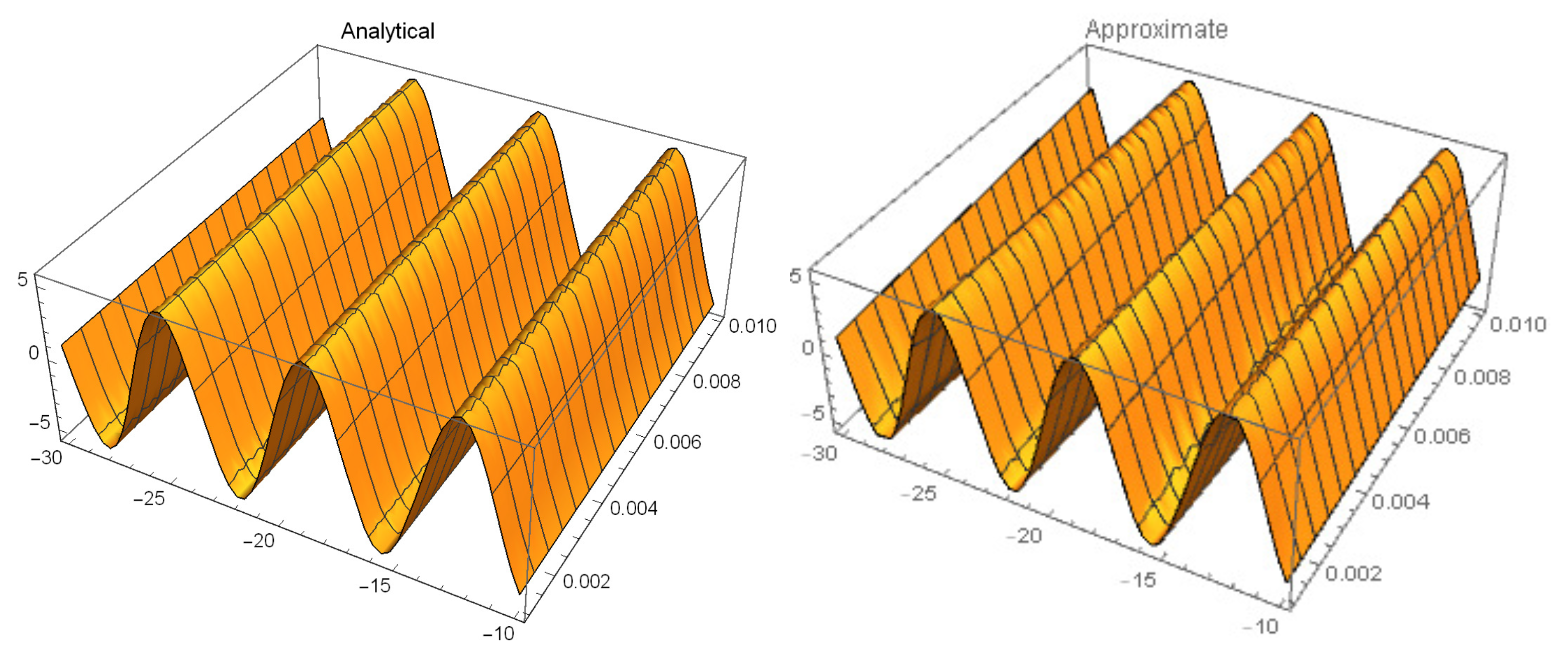
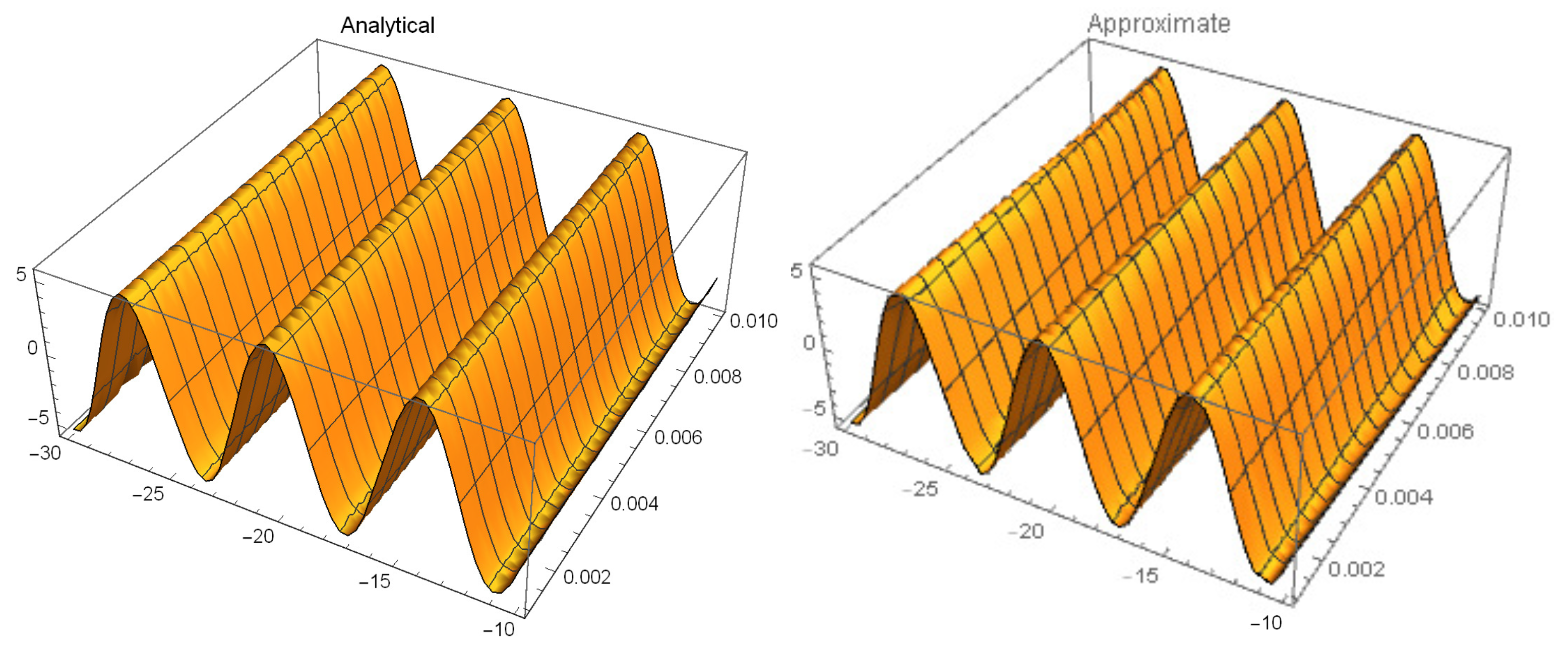
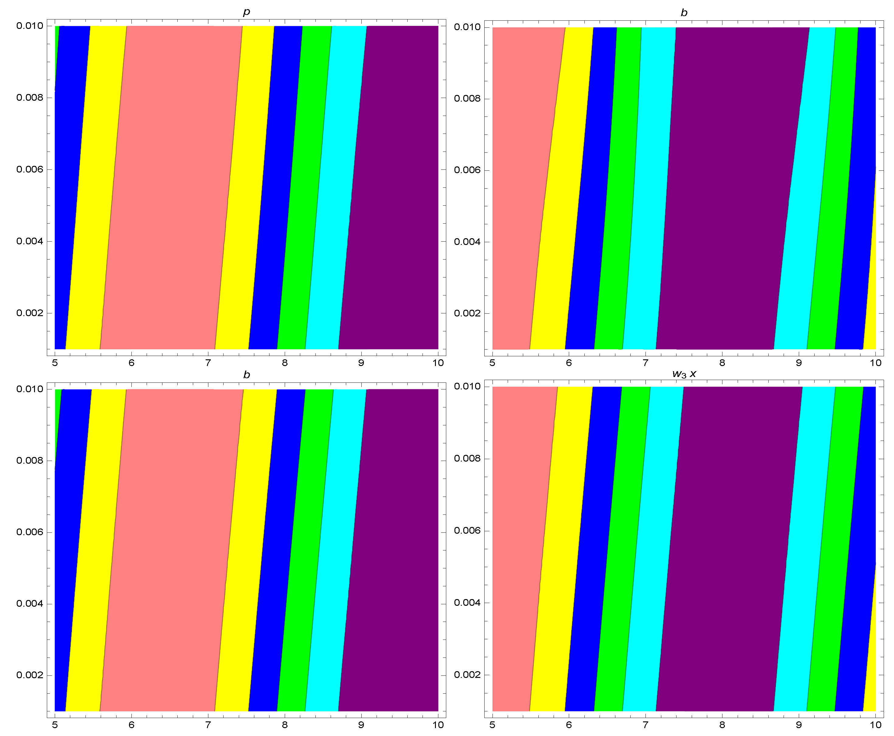
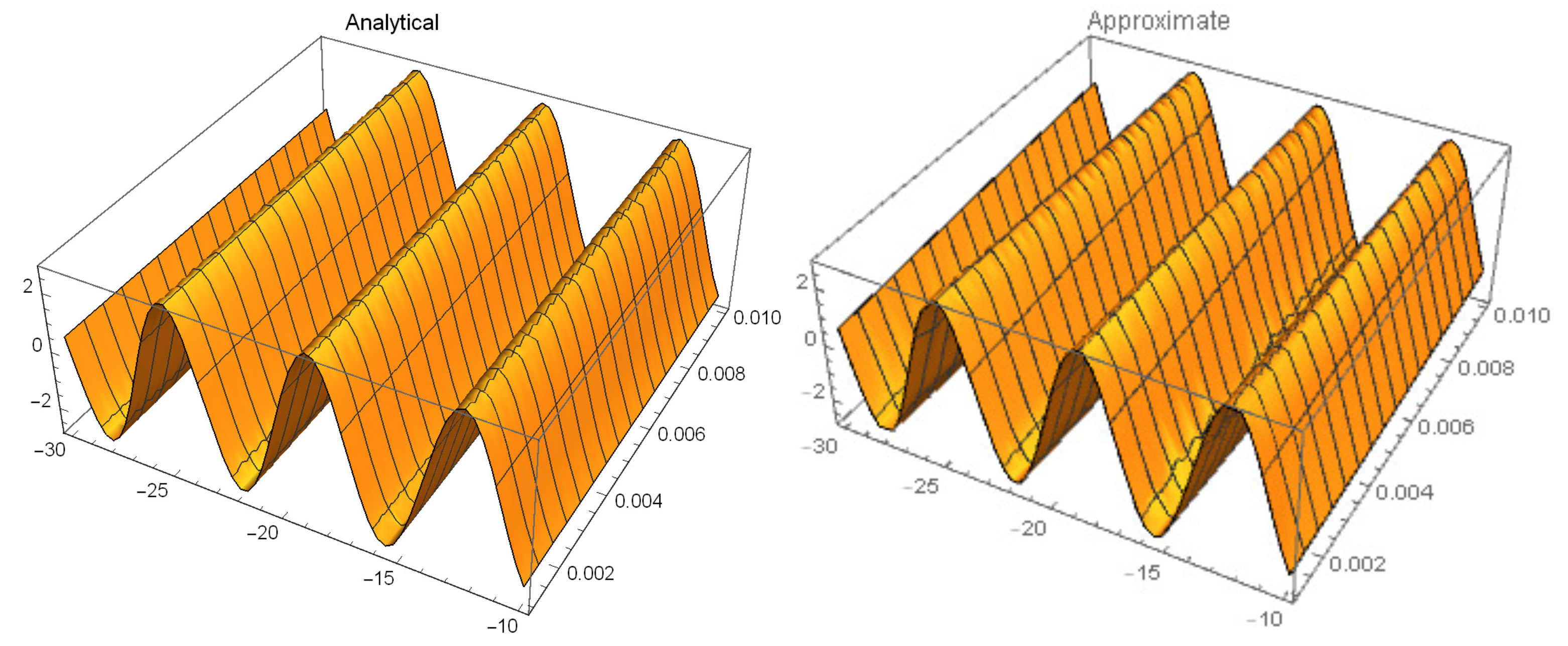
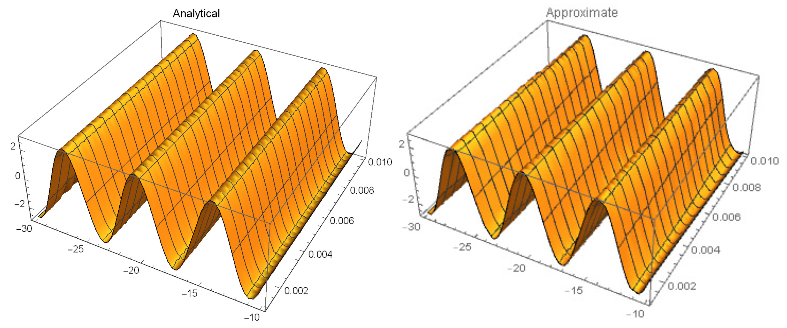
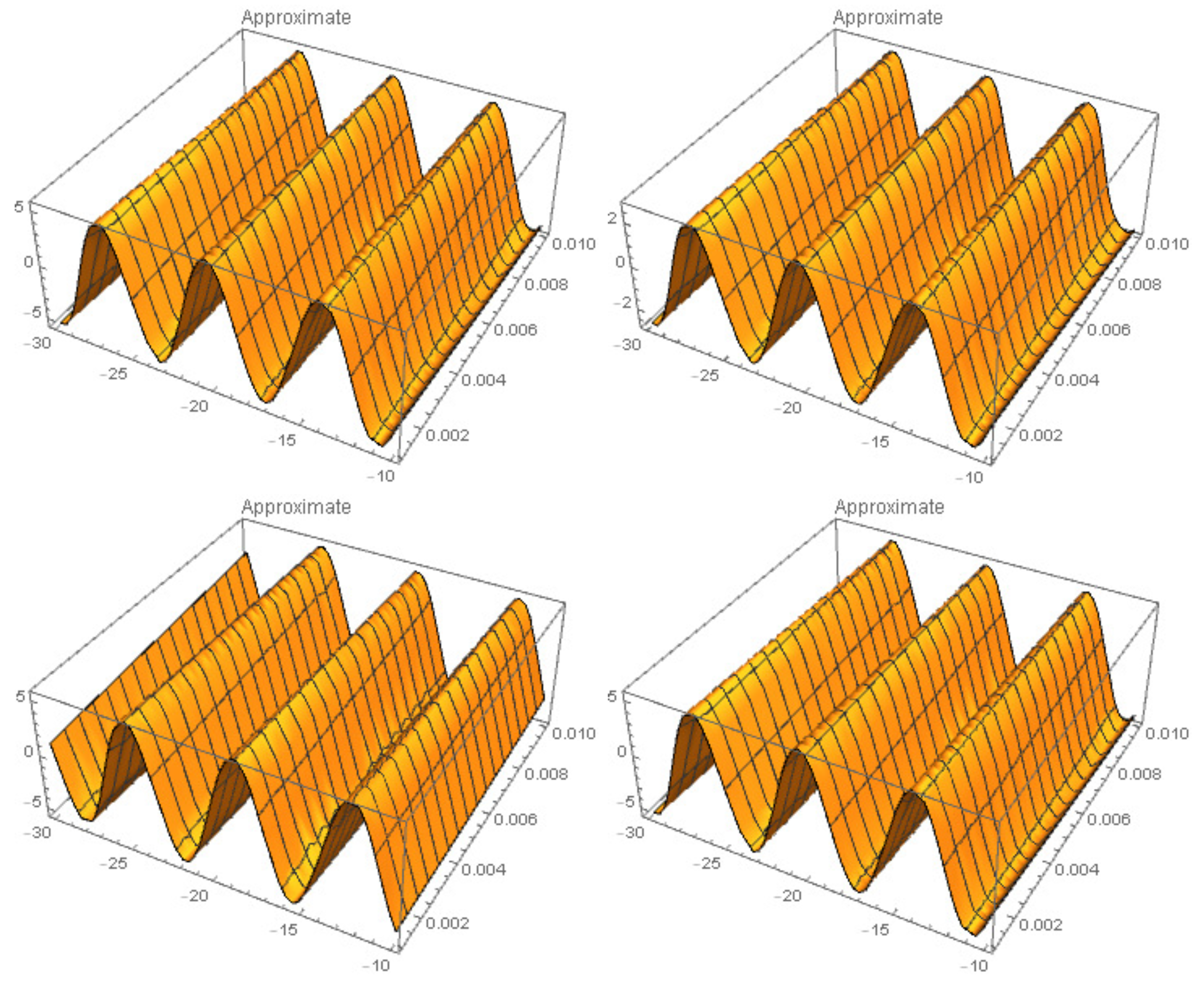
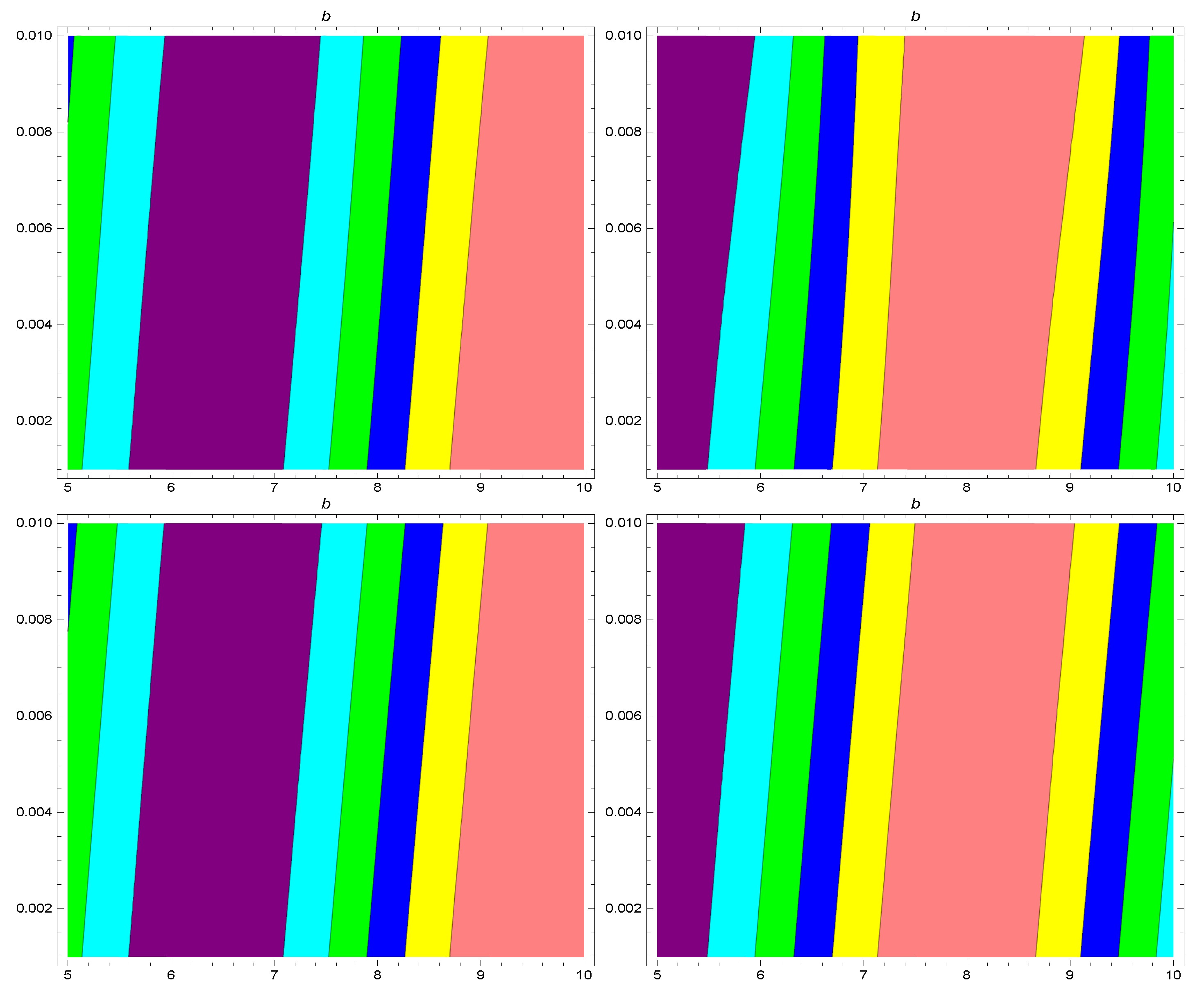
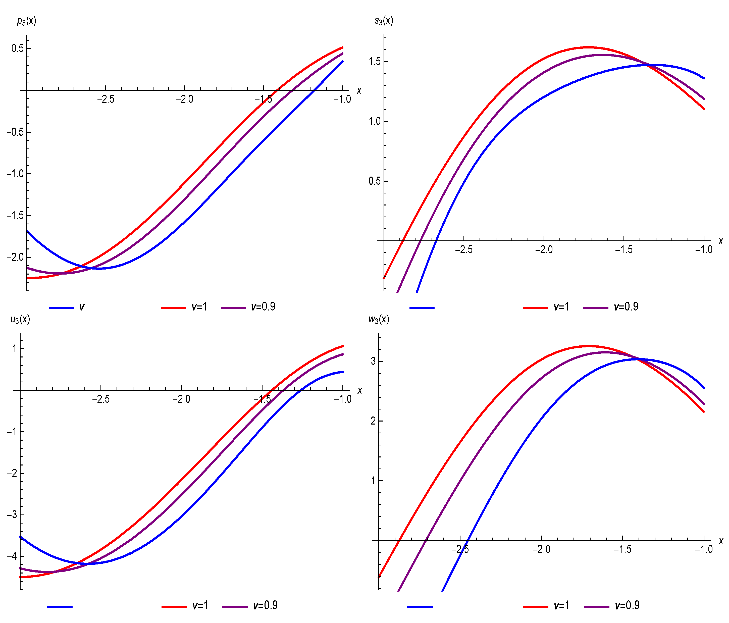
4. Graphical Representation

To depict the reliability of the RPST to obtain the optical solutions to fiber Bragg gratings with cubic–quartic dispersive reflectivity having the Kerr law of nonlinear refractive index structures, three applications are examined. The fractional derivative is defined by Caputo’s sense.

Example 1. 

Examine the system,

$$\begin{array}{cc}\hfill \iota D_t^{\varrho }n+\iota a_1{o}_{\varpi \varpi \varpi }+b_1{o}_{\varpi \varpi \varpi \varpi }+(c_1{\left|n\right|}^2+d_1{\left|o\right|}^2)n+\iota {\alpha }_1{n}_{\varpi }+{\beta }_{1}o=0,& \\ \hfill \iota D_t^{\varrho }o+\iota a_2{n}_{\varpi \varpi \varpi }+b_2{n}_{\varpi \varpi \varpi \varpi }+(c_2{\left|n\right|}^2+d_2{\left|n\right|}^2)o+\iota {\alpha }_2{o}_{\varpi }+{\beta }_{2}n=0,\end{array}$$

(22)

where $0<\varrho <1$, subject to the initial conditions,

$$\begin{array}{c}\hfill n(\varpi ,0)=\left({\left(\frac{-2A_3}{15k^2}\right)}^{\frac{-1}{6}}\left[({\gamma }_1-{\gamma }_2){tanh}^2\left(\frac{\sqrt{({\gamma }_1-{\gamma }_2)}}{2}\left({\left(\frac{-2A_3}{15k^2}\right)}^{\frac{-1}{6}}\xi -{\xi }_0\right)\right)+{\gamma }_2\right]\right){exp}^{\iota (-\kappa \varpi +\theta )},\end{array}$$

(23)

$$\begin{array}{c}\hfill o(\varpi ,0)=2\left({\left(\frac{-2A_3}{15k^2}\right)}^{\frac{-1}{6}}\left[({\gamma }_1-{\gamma }_2){tanh}^2\left(\frac{\sqrt{({\gamma }_1-{\gamma }_2)}}{2}\left({\left(\frac{-2A_3}{15k^2}\right)}^{\frac{-1}{6}}\xi -{\xi }_0\right)\right)+{\gamma }_2\right]\right){exp}^{\iota (-\kappa \varpi +\theta )}.\end{array}$$

(24)

This problem has an analytical solution for $\varrho =1$ that is provided in [17] as

$$\begin{array}{c}\hfill n(\varpi ,t)=\left({\left(\frac{-2A_3}{15k^2}\right)}^{\frac{-1}{6}}\left[({\gamma }_1-{\gamma }_2){tanh}^2\left(\frac{\sqrt{({\gamma }_1-{\gamma }_2)}}{2}\left({\left(\frac{-2A_3}{15k^2}\right)}^{\frac{-1}{6}}\xi -{\xi }_0\right)\right)+{\gamma }_2\right]\right){exp}^{\iota (-\kappa \varpi +\omega t+\theta )},\end{array}$$

(25)

$$\begin{array}{c}\hfill o(\varpi ,t)=2\left({\left(\frac{-2A_3}{15k^2}\right)}^{\frac{-1}{6}}\left[({\gamma }_1-{\gamma }_2){tanh}^2\left(\frac{\sqrt{({\gamma }_1-{\gamma }_2)}}{2}\left({\left(\frac{-2A_3}{15k^2}\right)}^{\frac{-1}{6}}\xi -{\xi }_0\right)\right)+{\gamma }_2\right]\right){exp}^{\iota (-\kappa \varpi +\omega t+\theta )}.\end{array}$$

(26)

For graphical observations, 2D plotting, contour plotting, and 3D plotting are constructed for Example 1 and shown in the Figure 1, Figure 2, Figure 3, Figure 4, Figure 5 and Figure 6. It can be seen that the power series solutions very accurately agreed with the analytical solutions. Finally, by employing a large number of terms from the residual power series approximations, a lower error can be attained. The 2D graphs for Example 1 illustrate that the solution had nearly identical behavior for the standard case $\varrho =1$ and various values of $\varrho$ in terms of accuracy.

Example 2. 

Examine the system

$$\begin{array}{cc}\hfill \iota D_t^{\varrho }n+\iota a_1{o}_{\varpi \varpi \varpi }+b_1{o}_{\varpi \varpi \varpi \varpi }+(c_1{\left|n\right|}^2+d_1{\left|o\right|}^2)n+\iota {\alpha }_1{n}_{\varpi }+{\beta }_{1}o=0,& \\ \hfill \iota D_t^{\varrho }o+\iota a_2{n}_{\varpi \varpi \varpi }+b_2{n}_{\varpi \varpi \varpi \varpi }+(c_2{\left|n\right|}^2+d_2{\left|n\right|}^2)o+\iota {\alpha }_2{o}_{\varpi }+{\beta }_{2}n=0,\end{array}$$

(27)

where $0<\varrho <1$, subject to the initial conditions

$$\begin{array}{c}\hfill n(\varpi ,0)=\left({\left(\frac{-2A_3}{15k^2}\right)}^{\frac{-1}{6}}\left[({\gamma }_1-{\gamma }_2){tanh}^2\left(\frac{\sqrt{({\gamma }_1-{\gamma }_2)}}{2}\left({\left(\frac{-2A_3}{15k^2}\right)}^{\frac{-1}{6}}\xi -{\xi }_0\right)\right)+{\gamma }_2\right]\right)\\ \hfill tanh(-\kappa \varpi +\theta ){exp}^{\iota (-\kappa \varpi +\theta )},\end{array}$$

(28)

$$\begin{array}{c}\hfill o(\varpi ,0)=2\left({\left(\frac{-2A_3}{15k^2}\right)}^{\frac{-1}{6}}\left[({\gamma }_1-{\gamma }_2){tanh}^2\left(\frac{\sqrt{({\gamma }_1-{\gamma }_2)}}{2}\left({\left(\frac{-2A_3}{15k^2}\right)}^{\frac{-1}{6}}\xi -{\xi }_0\right)\right)+{\gamma }_2\right]\right)\\ \hfill tanh(-\kappa \varpi +\theta ){exp}^{\iota (-\kappa \varpi +\theta )}.\end{array}$$

(29)

The advantage of using the RPST is that it establishes the continuous approximated solutions. In the Figure 7, Figure 8 and Figure 9, the power series generated solutions of (27) are depicted geometrically by 3D plotting, contour plotting and 2D plotting. Error can be reduced by taking many terms, and the efficiency of the method can be increased.

Example 3. 

Examine the system,

$$\begin{array}{cc}\hfill \iota D_t^{\varrho }n+\iota a_1{o}_{\varpi \varpi \varpi }+b_1{o}_{\varpi \varpi \varpi \varpi }+(c_1{\left|n\right|}^2+d_1{\left|o\right|}^2)n+\iota {\alpha }_1{n}_{\varpi }+{\beta }_{1}o=0,& \\ \hfill \iota D_t^{\varrho }o+\iota a_2{n}_{\varpi \varpi \varpi }+b_2{n}_{\varpi \varpi \varpi \varpi }+(c_2{\left|n\right|}^2+d_2{\left|n\right|}^2)o+\iota {\alpha }_2{o}_{\varpi }+{\beta }_{2}n=0,\end{array}$$

(30)

where $0<\varrho <1$, subject to the initial conditions,

$$\begin{array}{c}\hfill n(\varpi ,0)=\left({\left(\frac{-2A_3}{15k^2}\right)}^{\frac{-1}{6}}\left[({\gamma }_1-{\gamma }_2){tanh}^2\left(\frac{\sqrt{({\gamma }_1-{\gamma }_2)}}{2}\left({\left(\frac{-2A_3}{15k^2}\right)}^{\frac{-1}{6}}\xi -{\xi }_0\right)\right)+{\gamma }_2\right]\right)\\ \hfill sinh(-\kappa \varpi +\theta ){exp}^{\iota (-\kappa \varpi +\theta )},\end{array}$$

(31)

$$\begin{array}{c}\hfill o(\varpi ,0)=2\left({\left(\frac{-2A_3}{15k^2}\right)}^{\frac{-1}{6}}\left[({\gamma }_1-{\gamma }_2){tanh}^2\left(\frac{\sqrt{({\gamma }_1-{\gamma }_2)}}{2}\left({\left(\frac{-2A_3}{15k^2}\right)}^{\frac{-1}{6}}\xi -{\xi }_0\right)\right)+{\gamma }_2\right]\right)\\ \hfill sinh(-\kappa \varpi +\theta ){exp}^{\iota (-\kappa \varpi +\theta )}.\end{array}$$

(32)

Figure 10 represents the mathematical behavior of Equation (30) subject to initial conditions Equations (31) and (32). It can be clearly observed that the obtained solution also depends on the initial conditions. By varying the initial conditions, the mathematical behavior of a problem also changes. Consequently, the proposed technique is an effective technique for the approximated solutions of different fractional-order models.

5. Conclusions

In this paper, the RPST with Caputo’s time-fractional derivative is applied to develop the approximate solutions to FBGs with cubic–quartic dispersive reflectivity having the Kerr law of nonlinear refractive index, with high accuracy for the first time. The efficiency and reliability of the RPST are established by three test applications with different initial conditions. It is worth mentioning that the RPST structure has a rapidly converging series with components that are easily calculated with symbolic calculation software. The obtained results are also demonstrated through 2D and 3D representations by taking different values of $\varrho$. Since the exact solution of the problem for $\varrho =1$ is available in the literature, a graphical comparison is made to confirm that the RPS approximation solutions are in agreement with the exact solutions for $\varrho =1$. The variation in the solutions for change in the value of $\varrho$ is also observed. The consequence found by using the active RPST is that it can be successfully used to investigate the dynamics of nonlinear models in the field of optical fibers.

References

1. Biswas, A.; Fessak, M.; Johnson, S.; Beatrice, S.; Milovic, D.; Jovanoski, Z.; Majid, F. Optical soliton perturbation in non-Kerr law media: Traveling wave solution. Opt. Laser Technol. 2012, 44, 263–268. [Google Scholar] [CrossRef]
2. Kudryashov, N.A. Periodic and solitary waves in optical fiber Bragg gratings with dispersive reflectivity. Chin. J. Phys. 2020, 66, 401–405. [Google Scholar] [CrossRef]
3. Kan, K.V.; Kudryashov, N.A. Solitary waves described by a high-order system in optical fiber Bragg gratings with arbitrary refractive index. Math. Methods Appl. Sci. 2022, 45, 1072–1079. [Google Scholar] [CrossRef]
4. Zayed, E.M.; Nofal, T.A.; Gepreel, K.A.; Shohib, R.M.; Alngar, M.E. Cubic-quartic optical soliton solutions in fiber Bragg gratings with Lakshmanan-Porsezian-Daniel model by two integration schemes. Opt. Quantum Electron. 2021, 53, 249. [Google Scholar] [CrossRef]
5. Biswas, A.; Konar, S. Introduction to Non-Kerr Law Optical Solitons; Chapman and Hall/CRC: Boca Raton, FL, USA, 2006. [Google Scholar]
6. Zhou, Q.; Yao, D.; Xu, Q.; Liu, X. Optical soliton perturbation with time and space dependent dissipation (orgain) and nonlinear dispersion in Kerr and non-Kerr media. Optik 2013, 124, 2368–2372. [Google Scholar] [CrossRef]
7. Biswas, A.; Ekici, M.; Sonmezoglu, A.; Belic, M.R. Highly dispersive optical solitons with Kerr law nonlinearity by F-expansion. Optik 2019, 181, 1028–1038. [Google Scholar] [CrossRef]
8. Alkhidhr, H.A. Closed-form solutions to the perturbed NLSE with Kerr law nonlinearity in optical fibers. Results Phys. 2021, 22, 103875. [Google Scholar] [CrossRef]
9. Gunay, B. Optical soliton solutions to a higher-order nonlinear Schrödinger equation with Kerr law nonlinearity. Results Phys. 2021, 27, 104515. [Google Scholar] [CrossRef]
10. Malik, S.; Kumar, S.; Biswas, A.; Yildirim, Y.; Moraru, L.; Moldovanu, S.; Iticescu, C.; Moshokoa, S.P.; Bibicu, D.; Alotaibi, A. Gap Solitons in Fiber Bragg Gratings Having Polynomial Law of Nonlinear Refractive Index and Cubic-Quartic Dispersive Reflectivity by Lie Symmetry. Symmetry 2023, 15, 963. [Google Scholar] [CrossRef]
11. Triki, H.; Zhou, Q.; Biswas, A.; Liu, W.; Yildirim, Y.; Alshehri, H.M.; Belic, M.R. Chirped optical solitons having polynomial law of nonlinear refractive index with self-steepening and nonlinear dispersion. Phys. Lett. A 2021, 417, 127698. [Google Scholar] [CrossRef]
12. Zayed, E.M.; Shohib, R.M.; Alngar, M.E. Cubic-quartic optical solitons in Bragg gratings fibers for NLSE having parabolic non-local law nonlinearity using two integration schemes. Opt. Quantum Electron. 2021, 53, 452. [Google Scholar] [CrossRef]
13. Zayed, E.M.; Alngar, M.E.; El-Horbaty, M.; Biswas, A.; Alshomrani, A.S.; Khan, S.; Triki, H. Optical solitons in fiber Bragg gratings having Kerr law of refractive index with extended Kudryashov method and new extended auxiliary equation approach. Chin. J. Phys. 2020, 66, 187–205. [Google Scholar] [CrossRef]
14. Yildirim, Y.; Biswas, A.; Khan, S.; Guggilla, P.; Alzahrani, A.K.; Belic, M.R. Optical solitons in fiber Bragg gratings with dispersive reflectivity by sine-Gordon equation approach. Optik 2021, 237, 166684. [Google Scholar] [CrossRef]
15. Sahota, J.K.; Gupta, N.; Dhawan, D. Fiber Bragg grating sensors for monitoring of physical parameters: A comprehensive review. Opt. Eng. 2020, 59, 060901. [Google Scholar] [CrossRef]
16. Zhao, H.; Zhang, M.; Zhu, C.; Li, H. Multichannel fiber bragg grating based on DC-sampling method. Opt. Commun. 2019, 445, 142–146. [Google Scholar] [CrossRef]
17. Wang, M.Y.; Biswas, A.; Yildirim, Y.; Alshehri, H.M.; Moraru, L.; Moldovanu, S. Optical solitons in fiber Bragg gratings with dispersive reflectivity having five nonlinear forms of refractive index. Axioms 2022, 11, 640. [Google Scholar] [CrossRef]
18. Yildirim, Y.; Biswas, A.; Guggilla, P.; Khan, S.; Alshehri, H.M.; Belic, M.R. Optical solitons in fibre Bragg gratings with third and fourth order dispersive reflectivities. Ukr. J. Phys. Opt. 2021, 22, 239–254. [Google Scholar] [CrossRef]
19. Malik, S.; Kumar, S.; Biswas, A.; Yildirim, Y.; Moraru, L.; Moldovanu, S.; Iticescu, C.; Alshehri, H.M. Cubic-quartic optical solitons in fiber bragg gratings with dispersive reflectivity having parabolic law of nonlinear refractive index by lie symmetry. Symmetry 2022, 14, 2370. [Google Scholar] [CrossRef]
20. Arnous, A.H.; Zhou, Q.; Biswas, A.; Guggilla, P.; Khan, S.; Yildirim, Y.; Alshomrani, A.S.; Alshehri, H.M. Optical solitons in fiber Bragg gratings with cubic-quartic dispersive reflectivity by enhanced Kudryashov’s approach. Phys. Lett. A 2022, 422, 127797. [Google Scholar] [CrossRef]
21. Zayed, E.M.; Alngar, M.E.; Biswas, A.; Ekici, M.; Alzahrani, A.K.; Belic, M.R. Solitons in fiber Bragg gratings with cubic-quartic dispersive reflectivity having Kerr law of nonlinear refractive index. J. Nonlinear Opt. Phys. Mater. 2020, 29, 2050011. [Google Scholar] [CrossRef]
22. Podlubny, I. Fractional Differential Equations: An Introduction to Fractional Derivatives, Fractional Differential Equations, to Methods of Their Solution and Some of Their Applications; Elsevier: Amsterdam, The Netherlands, 1998. [Google Scholar]
23. Oldham, K.B.; Spanier, J. The Fractional Calculus; Academic Press: New York, NY, USA, 1974. [Google Scholar]
24. Sabatier, J.; Agrawal, O.P.; Machado, J.A.T. Advances in Fractional Calculus; Springer: Dordrecht, The Netherlands, 2007; Volume 4. [Google Scholar]
25. Tian, Q.; Yang, X.; Zhang, H.; Xu, D. An implicit robust numerical scheme with graded meshes for the modified Burgers model with nonlocal dynamic properties. Comput. Appl. Math. 2023, 42, 246. [Google Scholar] [CrossRef]
26. Guo, L.; Zhao, X.L.; Gu, X.M.; Zhao, Y.L.; Zheng, Y.B.; Huang, T.Z. Three-dimensional fractional total variation regularized tensor optimized model for image deblurring. Appl. Math. Comput. 2021, 404, 126224. [Google Scholar] [CrossRef]
27. Yang, X.; Wu, L.; Zhang, H. A space-time spectral order sinc-collocation method for the fourth-order nonlocal heat model arising in viscoelasticity. Appl. Math. Comput. 2023, 457, 128192. [Google Scholar] [CrossRef]
28. Jiang, X.; Wang, J.; Wang, W.; Zhang, H. A Predictor-Corrector Compact Difference Scheme for a Nonlinear Fractional Differential Equation. Fractal Fract. 2023, 7, 521. [Google Scholar] [CrossRef]
29. Wu, G.C. A fractional variational iteration method for solving fractional nonlinear differential equations. Comput. Math. Appl. 2011, 61, 2186–2190. [Google Scholar] [CrossRef]
30. Ganjiani, M. Solution of nonlinear fractional differential equations using homotopy analysis method. Appl. Math. Model. 2010, 34, 1634–1641. [Google Scholar] [CrossRef]
31. Hashim, D.J.; Jameel, A.F.; Ying, T.Y.; Alomari, A.K.; Anakira, N.R. Optimal homotopy asymptotic method for solving several models of first order fuzzy fractional IVPs. Alex. Eng. J. 2022, 61, 4931–4943. [Google Scholar] [CrossRef]
32. Nadeem, M.; He, J.H.; Islam, A. The homotopy perturbation method for fractional differential equations: Part 1 Mohand transform. Int. J. Numer. Methods Heat Fluid Flow 2021, 31, 3490–3504. [Google Scholar] [CrossRef]
33. Alkresheh, H.A.; Ismail, A.I. Multi-step fractional differential transform method for the solution of fractional order stiff systems. Ain Shams Eng. J. 2021, 12, 4223–4231. [Google Scholar] [CrossRef]
34. Zhang, Q.; Qin, Y.; Sun, Z.Z. Linearly compact scheme for 2D Sobolev equation with Burgers’ type nonlinearity. Numer. Algorithms 2022, 91, 1081–1114. [Google Scholar] [CrossRef]
35. Jafari, H.; Daftardar-Gejji, V. Solving a system of nonlinear fractional differential equations using Adomian decomposition. J. Comput. Appl. Math. 2006, 196, 644–651. [Google Scholar] [CrossRef]
36. Korpinar, T.; Korpinar, Z. Approximate solutions for optical magnetic and electric phase with fractional optical Heisenberg ferromagnetic spin by RPSM. Optik 2021, 247, 167819. [Google Scholar] [CrossRef]
37. Tariq, H.; Akram, G. Residual power series method for solving time-space-fractional Benney-Lin equation arising in falling film problems. J. Appl. Math. Comput. 2017, 55, 683–708. [Google Scholar] [CrossRef]
38. Burqan, A.; Saadeh, R.; Qazza, A.; Momani, S. ARA-residual power series method for solving partial fractional differential equations. Alex. Eng. J. 2023, 62, 47–62. [Google Scholar] [CrossRef]
39. Saadeh, R. A reliable algorithm for solving system of multi-pantograph equations. WSEAS Trans. Math 2022, 21, 792–800. [Google Scholar] [CrossRef]
40. Ismail, G.M.; Abdl-Rahim, H.R.; Ahmad, H.; Chu, Y.M. Fractional residual power series method for the analytical and approximate studies of fractional physical phenomena. Open Phys. 2020, 18, 799–805. [Google Scholar] [CrossRef]
41. Arqub, O.A. Series solution of fuzzy differential equations under strongly generalized differentiability. J. Adv. Res. Appl. Math 2013, 5, 31–52. [Google Scholar] [CrossRef]
42. Wang, L.; Chen, X. Approximate analytical solutions of time fractional Whitham-Broer-Kaup equations by a residual power series method. Entropy 2015, 17, 6519–6533. [Google Scholar] [CrossRef]
43. Dubey, V.P.; Kumar, R.; Kumar, D. A reliable treatment of residual power series method for time-fractional Black-Scholes European option pricing equations. Phys. A Stat. Mech. Its Appl. 2019, 533, 122040. [Google Scholar] [CrossRef]
44. Senol, M.; Ata, A. Approximate solution of time-fractional KdV equations by residual power series method. BAUN Fen Bil. Enst. Dergisi 2018, 20, 430–439. [Google Scholar] [CrossRef]
45. Tariq, H.; Sadaf, M.; Akram, G.; Rezazadeh, H.; Baili, J.; Lv, Y.P.; Ahmad, H. Computational study for the conformable nonlinear Schrödinger equation with cubic-quintic-septic nonlinearities. Results Phys. 2021, 30, 104839. [Google Scholar] [CrossRef]
46. Korpinar, Z.; Inc, M. Numerical simulations for fractional variation of (1 + 1)-dimensional Biswas-Milovic equation. Optik 2018, 166, 77–85. [Google Scholar] [CrossRef]
47. Tariq, H.; Ahmed, H.; Rezazadeh, H.; Javeed, S.; Alimgeer, K.S.; Nonlaopon, K.; Khedher, K.M. New travelling wave analytic and residual power series solutions of conformable Caudrey-Dodd-Gibbon-Sawada-Kotera equationequation. Results Phys. 2021, 29, 104591. [Google Scholar] [CrossRef]
48. Tariq, H.; Akram, G. New traveling wave exact and approximate solutions for the nonlinear Cahn-Allen equation: Evolution of a nonconserved quantity. Nonlinear Dyn. 2017, 88, 581–594. [Google Scholar] [CrossRef]
49. Kumar, S.; Kumar, A.; Baleanu, D. Two analytical methods for time-fractional nonlinear coupled Boussinesq-Burger’s equations arise in propagation of shallow water waves. Nonlinear Dyn. 2016, 85, 699–715. [Google Scholar] [CrossRef]
Figure 1. Two-dimensional (2D) graphs of the 3rd residual power series solutions with various values of ϱ for Example 1 with A 3 = 1 , k = 1 , γ 1 = 2 , γ 2 = 1 , ξ 0 = 0 , κ = 1 , t = 0.01 , and θ = 0 .
Fractalfract 07 00625 g001
Figure 2. Contour plots for the 3rd residual power series solutions p 3 ( ϖ , t ) , s 3 ( ϖ , t ) , u 3 ( ϖ , t ) , and w 3 ( ϖ , t ) with various values of ϱ for Example 1 with A 3 = 1 , k = 1 , γ 1 = 2 , γ 2 = 1 , ξ 0 = 0 , κ = 1 , t = 0.01 , and θ = 0 .
Fractalfract 07 00625 g002
Figure 3. Three-dimensional (3D) surface plots of analytical solution and approximate solutions p 3 ( ϖ , t ) at ϱ = 1 of Example 1 with A 3 = 1 , k = 1 , γ 1 = 2 , γ 2 = 1 , ξ 0 = 0 , κ = 1 , and θ = 0 .
Fractalfract 07 00625 g003
Figure 4. Three-dimensional (3D) surface plots of analytical solution and approximate solutions s 3 ( ϖ , t ) at ϱ = 1 of Example 1 with A 3 = 1 , k = 1 , γ 1 = 2 , γ 2 = 1 , ξ 0 = 0 , κ = 1 , and θ = 0 .
Fractalfract 07 00625 g004
Figure 5. Three-dimensional (3D) surface plots of analytical solution and approximate solutions u 3 ( ϖ , t ) at ϱ = 1 of Example 1 with A 3 = 1 , k = 1 , γ 1 = 2 , γ 2 = 1 , ξ 0 = 0 , κ = 1 , and θ = 0 .
Fractalfract 07 00625 g005
Figure 6. Three-dimensional (3D) surface plots of analytical solution and approximate solutions w 3 ( ϖ , t ) at ϱ = 1 of Example 1 with A 3 = 1 , k = 1 , γ 1 = 2 , γ 2 = 1 , ξ 0 = 0 , κ = 1 , and θ = 0 .
Fractalfract 07 00625 g006
Figure 7. Three-dimensional (3D) surface plots approximate solutions p 3 ( ϖ , t ) , s 3 ( ϖ , t ) , u 3 ( ϖ , t ) , and w 3 ( ϖ , t ) at ϱ = 1 of Example 2 with A 3 = 1 , k = 1 , γ 1 = 2 , γ 2 = 1 , ξ 0 = 0 , κ = 1 , and θ = 0 .
Fractalfract 07 00625 g007
Figure 8. Contour plots for the 3rd residual power series solutions with various values of ϱ for Example 2 with A 3 = 1 , k = 1 , γ 1 = 2 , γ 2 = 1 , ξ 0 = 0 , κ = 1 , t = 0.01 , and θ = 0 .
Fractalfract 07 00625 g008
Figure 9. Two-dimensional (2D) graphs of the 3rd residual power series solutions p 3 ( ϖ , t ) , s 3 ( ϖ , t ) , u 3 ( ϖ , t ) , and w 3 ( ϖ , t ) with various values of ϱ for Example 2 with A 3 = 1 , k = 1 , γ 1 = 2 , γ 2 = 1 , ξ 0 = 0 , κ = 1 , t = 0.01 , and θ = 0 .
Fractalfract 07 00625 g009
Figure 10. Two-dimensional (2D) graphs of the 3rd residual power series solutions with various values of ϱ for Example 3 with A 3 = 1 , k = 1 , γ 1 = 2 , γ 2 = 1 , ξ 0 = 0 , κ = 1 , t = 0.01 , and θ = 0 .
Fractalfract 07 00625 g010
Disclaimer/Publisher’s Note: The statements, opinions and data contained in all publications are solely those of the individual author(s) and contributor(s) and not of MDPI and/or the editor(s). MDPI and/or the editor(s) disclaim responsibility for any injury to people or property resulting from any ideas, methods, instructions or products referred to in the content.