Applying the DEMATEL Method to Analyze the Influence of Different Grey Accumulated Generating Operators on Samples

Abstract

Since the introduction of the grey forecasting model, various improvements have been developed in the field of grey accumulated generating operators (AGOs). Fractional accumulated generating operator (FAGO) and other novel AGOs have enriched the grey theory and expanded its application scope. Nevertheless, limited attention has been given to interrelationships and contributions of new and old information. To fill this research gap, this study employed the DEMATEL method to calculate the influence degree of samples under different grey AGOs. Additionally, the pattern of influence degree variation with respect to the accumulation order was determined. The results demonstrate that, compared to traditional first-order AGO, FAGO and its corresponding grey forecasting models can effectively utilize the advantages of new information by altering the accumulation order.

1. Introduction

Accurate and efficient forecasting is an indispensable and crucial part of the management decision-making process. In recent years, various predictive analysis methods have emerged, including forecasting models suitable for big data, such as regression forecasting [1], and neural network models, according to intelligent optimization algorithms [2], etc. Nevertheless, obtaining sufficient sample data is often challenging in many real-world scenarios. In comparison to forecasting methods that require a massive amount of data, the grey forecasting model achieves reliable predictive results with only a small amount of data. The grey forecasting model originates from research on nonlinear and uncertain problems. By performing accumulation generation and modeling on data sequences, it can extract useful information from a small amount of data and make effective predictions [3]. Compared to other methods, the grey forecasting model offers several advantages: (1) it exhibits strong capability in handling small sample data or missing data; (2) the model is simple, computationally convenient, and suitable for rapid prediction; (3) it can capture inherent patterns and trends within a system. Therefore, it has gained extensive applications in diverse social science fields. For example, in the economic domain, it can be employed to predict stock prices [4], energy prices [5], economic growth rates [6], etc. In environmental science, it can be utilized to assess air quality [7], water resource utilization [8], energy consumption [9], etc.

Since Deng [10] proposed the grey prediction model in 1982, numerous scholars have made significant improvements to the model from various perspectives. Research efforts have primarily concentrated on optimizing background values and initial conditions [11,12], transforming functions [13], adjusting residual errors through the incorporation of correction factors [14,15,16], and enhancing the accumulated generating operator (AGO) [17,18,19]. As a data transformation method, AGO is an essential component that distinguishes the grey model from other theories and holds a crucial position within the grey prediction model. By applying AGO, the original data can be transformed into accumulated values. The traditional grey prediction model employs the first-order accumulated generating operator (1-AGO) to preprocess the original data and enhance the regularity of the fitting sequence. However, the 1-AGO imposes restrictions on the forecasting ability of the grey model in nonlinear problems, and its fixed model structure also reduces its applicability in complex systems [20]. To enhance the stability of the model solution and obtain more accurate forecasting results, it is necessary to fully exploit the advantages of new information in the data [21]. Consequently, many researchers endeavored to improve the effectiveness of the grey AGOs, thus expanding the application scope of the grey model. FAGO reveals the trend of changes in the original data by performing fractional accumulation. It can handle nonlinear data and reveal trends in complex or irregular data.

Table 1. Research process regarding grey AGOs.

Author’s Information	AGOs	Contribution
Wu (2013) [17]	Fractional accumulated generating operator (FAGO)	Reducing inherent randomness in data and enhancing the performance of the model for nonlinear forecasting problems.
Chen (2020) [22]	Fractional Hausdorff accumulated generating operator (FHAGO)	Improving the predictive accuracy of traditional grey model and validating its applicability through three cases.
Ma (2020) [23]	Conformable fractional accumulated generating operator (CFAGO)	Predicting natural gas consumption in 11 countries to demonstrate its higher efficiency in long-term and non-stationary time series prediction.
Zhou (2017) [24]	New information priority accumulated generating operator (NIPAGO)	Further reflecting the information priority and validating the effectiveness of the model.
Liu (2021) [25]	Damping accumulated generating operator (DAGO)	Flexibly adjusting the trend component and correcting the results and validating the applicability through four cases.
Zhu (2022) [26]	Weakened fractional order accumulated generating operator (WFAGO)	Reducing the ill-condition of the discrete grey system and improving its performance and verifying the feasibility by predicting electricity consumption in Zhejiang and Heilongjiang.
Zhao (2020) [19]	Adjacent accumulated generating operator (AAGO)	Demonstrating its stability and high predictive accuracy, predicting the renewable energy consumption in the Asia–Pacific Economic Cooperation region.
Xiao (2017) [27]	Cycle truncation accumulated generating operator (CAGO)	Converting the traffic flow sequence of seasonal fluctuation into a flat sequence and verifying performance through predicting the traffic flow in China and Canada.
Li (2022) [28]	Generalized accumulated generating operator (GAGO)	Introducing a new information priority generalized accumulative grey model and forecasting greenhouse gas emissions in Shanghai Cooperation Organization member states.
Guo (2021) [29]	Quarterly compound accumulated generating operator (QAGO)	Introducing two seasonal parameters into the model and forecasting air quality in 22 cities.
Che (2013) [30]	Opposite-direction accumulated generating operator (OAGO)	Making full use of the new information and validating its applicability by predicting fatigue experimental data of Ti alloy.

presents the research process regarding grey AGOs.

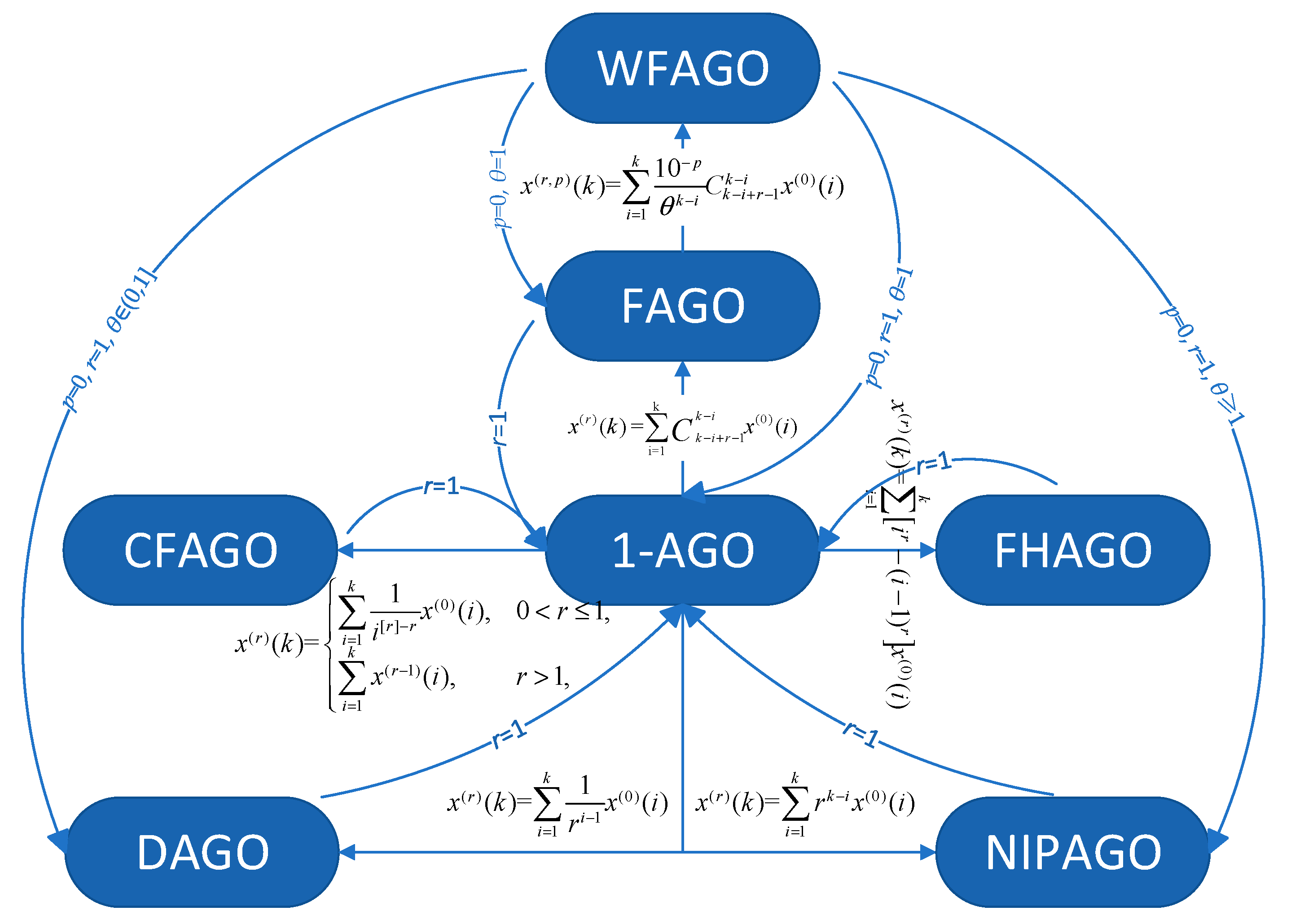
The above AGOs have significantly enriched grey theory and expanded the application scope of grey forecasting models. Nevertheless, there are still deficiencies in the research about the mathematical theoretical analysis of these AGOs. To investigate the difference in the utilization of new and old information under different AGOs, this paper adopts the decision-making trial and evaluation laboratory (DEMATEL) method to calculate the influence degree of each sample after accumulation. The DEMATEL method allows for the quantification of interrelationships and contributions between various factors in the system. This provides a more comprehensive understanding of the interactions among different AGOs and facilitates the evaluation of their importance in predicting model outcomes. The selected AGOs in this study are FAGO, FHAGO, CFAGO, NIPAGO, DAGO, and WFAGO, as illustrated in Figure 1.

The rest of this paper is organized as follows: Section 2 outlines the process of using the DEMATEL method to calculate the influence degree and presents the coefficient matrix of different AGOs. Section 3 analyzes the variations in influence degree between new and old information under various accumulation methods. Section 4 summarizes the variation regularity of the influence degree resulting from different accumulation orders and offers relevant suggestions accordingly.

2. Method and Model

2.1. The Grey Forecasting Model

The grey forecasting model is typically used for modeling and forecasting data with exponential growth patterns. Its core steps include data accumulation, equalization, the establishment of a differential equation, parameter estimation, and model testing. AGO facilitates the transformation of non-stationary time series into stationary sequences through accumulation, thereby enhancing the modeling and prediction processes. Improved AGOs have evolved to address different growth trends within time series, enabling a more effective capture of underlying tendencies. The whitening differential equation serves as a mathematical transformation aimed at enhancing estimation accuracy. The integration of AGO and whitening differential equations confers grey models with improved versatility and adaptability, resulting in better performance in modeling and prediction.

The GM(1,1) is a commonly used grey forecasting model. It utilizes the 1-AGO for modeling and forecasting. The original sequence is $X^{(0)}=\{x^{(0)}(1),x^{(0)}(2),\cdots ,x^{(0)}\left(\mathrm{n}\right)\}$. The 1-AGO sequence $X^{(1)}=\{x^{(1)}(1),x^{(1)}(2),\cdots ,x^{\left(1\right)}\left(\mathrm{n}\right)\}$ is obtained by $x^{(1)}(k)={\displaystyle \sum _{i=1}^k{x}^{(0)}(i)}$, $k=1,2,\cdots ,n$. Subsequently, the white differential equation is established using the accumulated sequence, enabling data fitting and prediction in a more accessible manner.

It is important to note that the GM(1,1) model is primarily suitable for data with exponential growth patterns and may not perform well for data with non-exponential growth. Additionally, it relies on the assumption of linear relationships and may not fit well for data with nonlinear relationships. Moreover, in the process of model selection, it is important to evaluate and validate the suitability of the model based on the specific problem at hand.

2.2. Different Grey AGOs and Coefficient Matrix

The original sequence is given as $X^{(0)}=\{x^{(0)}(1),x^{(0)}(2),\cdots ,x^{(0)}\left(\mathrm{n}\right)\}$. The r-order FAGO sequence of $X^{(r)}=\{x^{(r)}(1),x^{(r)}(2),\cdots ,x^{\left(r\right)}\left(\mathrm{n}\right)\}$ is obtained by the accumulative formula:

$$x^{(r)}(k)={\displaystyle \sum _{i=1}^k{{\displaystyle C}}_{k-i+r-1}^{k-i}}{x}^{(0)}(i)$$

(1)

where ${{\displaystyle C}}_{r-1}^0=1$, ${{\displaystyle C}}_k^{k+1}=0$, ${{\displaystyle C}}_{k-i+r-1}^{k-i}=\frac{(k-i+r-1)(k-i+r-2)\cdots (r+1)r}{(k-i)!}$, $k=1,2,\cdots ,n$.

According to Equation (1), the coefficient matrix under FAGO is

$$\left(\begin{array}{ccccc}0& C_r^1& \cdots & C_{n+r-3}^{n-2}& C_{n+r-2}^{n-1}\\ 0& 0& \cdots & C_{n+r-4}^{n-3}& C_{n+r-3}^{n-2}\\ ⋮& ⋮& ⋮& ⋮& ⋮\\ 0& 0& \cdots & 0& C_r^1\\ 0& 0& \cdots & 0& 0\end{array}\right)$$

(2)

The r-order accumulation sequence of the fractional Hausdorff grey model is obtained by FHAGO on the original sequence. The FHAGO sequence is

$$x^{(r)}(k)={\displaystyle \sum _{i=1}^k\left[i^r-{(i-1)}^r\right]}{x}^{(0)}(i),k=1,2,\cdots ,n.$$

(3)

The coefficient matrix under FHAGO is

$$\left(\begin{array}{ccccc}0& 1& \cdots & 1& 1\\ 0& 0& \cdots & 2^r-1& 2^r-1\\ ⋮& ⋮& ⋮& ⋮& ⋮\\ 0& 0& \cdots & 0& {(n-1)}^r-{(n-2)}^r\\ 0& 0& \cdots & 0& 0\end{array}\right)$$

(4)

The conformable fractional grey model proposes CFAGO to predict more effectively in long-term forecasts and non-smooth time series [23]. Based on the original sequence, the CFAGO is applied to obtain the r-order accumulation sequence of the conformable fractional grey model. The CFAGO sequence is

$$x^{(r)}(k)=\left\{\begin{array}{l}{\displaystyle \sum _{i=1}^k\frac{1}{i^{[r]-r}}}{x}^{(0)}(i), 0<r\le 1,\\ {\displaystyle \sum _{i=1}^k{x}^{(r-1)}(i)}, r>1,\end{array}\right.k=1,2,\cdots ,n.$$

(5)

where [r] is the smallest integer greater than or equal to r. When r is close to 1, the CFAGO sequence is close to the 1-AGO sequence, and when r is close to 2, the conformable fractional accumulation sequence is close to the second-order accumulated generating operator (2-AGO) sequence.

When $0<r\le 1$, the coefficient matrix under CFAGO is

$$\left(\begin{array}{ccccc}0& 1& \cdots & 1& 1\\ 0& 0& \cdots & \frac{1}{2^{[r]-r}}& \frac{1}{2^{[r]-r}}\\ ⋮& ⋮& ⋮& ⋮& ⋮\\ 0& 0& \cdots & 0& \frac{1}{{(n-1)}^{[r]-r}}\\ 0& 0& \cdots & 0& 0\end{array}\right)$$

(6)

When $r>1$, the coefficient matrix under CFAGO is

$$\left(\begin{array}{ccccc}0& C_{[r]}^1& \cdots & C_{n+[r]-3}^{n-2}& C_{n+[r]-2}^{n-1}\\ 0& 0& \cdots & \frac{C_{n+[r]-4}^{n-3}}{2^{[r]-r}}& \frac{C_{n+[r]-3}^{n-2}}{2^{[r]-r}}\\ ⋮& ⋮& ⋮& ⋮& ⋮\\ 0& 0& \cdots & 0& \frac{C_{[r]}^1}{{(n-1)}^{[r]-r}}\\ 0& 0& \cdots & 0& 0\end{array}\right)$$

(7)

The r-order accumulation sequence of the new information priority grey model is obtained by NIPAGO on the original sequence. The NIPAGO sequence is

$$x^{(r)}(k)={\displaystyle \sum _{i=1}^k{r}^{k-i}}{x}^{(0)}(i),k=1,2,\cdots ,n.$$

(8)

The coefficient matrix under NIPAGO is

$$\left(\begin{array}{ccccc}0& r& \cdots & r^{n-2}& r^{n-1}\\ 0& 0& \cdots & r^{n-3}& r^{n-2}\\ ⋮& ⋮& ⋮& ⋮& ⋮\\ 0& 0& \cdots & 0& r\\ 0& 0& \cdots & 0& 0\end{array}\right)$$

(9)

Based on the original sequence, the DAGO is applied to obtain the r-order accumulation sequence of the damping grey model. The DAGO sequence is

$$x^{(r)}(k)={\displaystyle \sum _{i=1}^k\frac{1}{r^{i-1}}}{x}^{(0)}(i),k=1,2,\cdots ,n.$$

(10)

The coefficient matrix under DAGO is

$$\left(\begin{array}{ccccc}0& 1& \cdots & 1& 1\\ 0& 0& \cdots & \frac{1}{r}& \frac{1}{r}\\ ⋮& ⋮& ⋮& ⋮& ⋮\\ 0& 0& \cdots & 0& \frac{1}{r^{n-2}}\\ 0& 0& \cdots & 0& 0\end{array}\right)$$

(11)

The r-order accumulation sequence of the weakened fractional grey model is obtained by WFAGO on the original sequence. The WFAGO sequence is

$$x^{(r,p)}(k)={\displaystyle \sum _{i=1}^k\frac{{10}^{-p}}{{\theta }^{k-i}}}{C}_{k-i+r-1}^{k-i}{x}^{(0)}(i),k=1,2,\cdots ,n.$$

(12)

where θ and p are the parameters to control the swift growth trend of the data. Zhu et al. utilized the examples of electricity consumption in Heilongjiang and Zhejiang to demonstrate the superiority of WFAO over other AGOs in terms of predictive performance and system ill-condition [26]. WFAGO combines multiplicative transformation with the modified FAGO. It can reduce initial data size through multiplicative transformation and adapt to different time series by adjusting hyperparameters. This flexibility and adaptability highlight the effectiveness of WFAGO in various applications. The existing 1-AGO, r-AGO, NIPAO, and DAGO are all special forms of WFAO. When the parameters p, r, and θ take different values, WFAGO can degenerate into 1-AGO (p = 0, r = 1, θ = 1), FAGO (p = 0, θ = 1), NIPAGO (p = 0, r = 1, θ ≥ 1), and DAGO (p = 0, r = 1, θ∈(0,1]), respectively.

The coefficient matrix under WFAGO is

$$\left(\begin{array}{ccccc}0& C_r^1\frac{{10}^{-p}}{{\theta }^{}}& \cdots & C_{n+r-3}^{n-2}\frac{{10}^{-p}}{{\theta }^{n-2}}& C_{n+r-2}^{n-1}\frac{{10}^{-p}}{{\theta }^{n-1}}\\ 0& 0& \cdots & C_{n+r-4}^{n-3}\frac{{10}^{-p}}{{\theta }^{n-3}}& C_{n+r-3}^{n-2}\frac{{10}^{-p}}{{\theta }^{n-2}}\\ ⋮& ⋮& ⋮& ⋮& ⋮\\ 0& 0& \cdots & 0& C_r^1\frac{{10}^{-p}}{{\theta }^{}}\\ 0& 0& \cdots & 0& 0\end{array}\right)$$

(13)

By utilizing the coefficient matrix for various AGOs, the influence degree of each operator can be calculated. The calculation steps are described in Section 2.4. The comparison of different AGOs is shown in

Table 2. The comparison of different AGOs.

AGOs	Advantages	Disadvantages
FAGO	It can handle nonlinear data and reveal trends in complex or irregular data.	High computational requirements.
FHAGO	It can satisfy the high stability of the model solution and simplify the integration operation process.	Unable to utilize initial value
CFAGO	It can maintain data consistency and stability, possess linear characteristics, and have relatively simple calculations.	Significant errors may occur when dealing with non-linear data.
NIPAGO	It assigns increasing weights to historical data through series operations to ensure that new data has greater importance than old data.	The contribution of older data may be excessively disregarded.
DAGO	During the accumulation process, each data point is given the same weight, so that the accumulation sequence still has monotonicity.	There may be significant errors for non-linear data.
WFAGO	It can alleviate the pathological state of the system by reducing the differences between system elements.	High computational requirements.

.

2.3. The DEMATEL Method

DEMATEL is an analytical approach for the analysis of various factors in a system, developed by the Battelle Institute [31]. This method combines graph theory and matrix tools and constructs a direct impact matrix based on the logic relations among the system elements. By describing the interrelationships of each element, the influence factors can be identified [32]. As an effective method to evaluate and identify the causal relationships between elements, it has been widely used to study the interactions in complex systems [33,34,35]. The existing literature on DEMATEL analysis mainly focuses on its development and improvement. In addition, hybrid models combining it with techniques such as grey model [36], analytic network process [37], or fuzzy logic [38] were proposed and studied. These studies provide insights into the relative performance and applicability of DEMATEL in different contexts. In this study, we introduce the application of DEMATEL to analyze AGOs in complex grey systems, demonstrating the practicality of this method in this new scenario. This paper uses the DEMATEL method to analyze the information priority. To facilitate understanding, we only select the influence degree to measure and investigate.

2.4. Influence Degree Calculation

The coefficient matrix of the grey model is used as the direct relation matrix of DEMATEL. In consideration of rationality, it is assumed that new information has no influence on old information, and thus its influence degree is assigned as 0. For example, the influence degree of $x^{(0)}(2)$ on $x^{(0)}(1)$ is considered to be 0, and similarly, the influence degree of $x^{(0)}(3)$ on both $x^{(0)}(1)$ and $x^{(0)}(2)$ is also 0. Moreover, the influence degree of each sample on itself is recorded as 0. For instance, the influence degree of $x^{(0)}(1)$ on itself is 0.

Taking five samples under 1-AGO as an example, the influence of each sample in $X^{(0)}=\{x^{(0)}(1),x^{(0)}(2),x^{(0)}(3),x^{(0)}(4),x^{(0)}\left(5\right)\}$ can be calculated, the calculation process is as follows.

Step 1: The direct relation matrix is generated by the coefficient matrix of the 1-AGO, as shown in

Table 3. The direct relation matrix A.

	x(0) (1)	x(0) (2)	x(0) (3)	x(0) (4)	x(0) (5)
x(0) (1)	0	1	1	1	1
x(0) (2)	0	0	1	1	1
x(0) (3)	0	0	0	1	1
x(0) (4)	0	0	0	0	1
x(0) (5)	0	0	0	0	0

.

Step 2: The direct relation matrix is normalized by summing each row in matrix A and taking the maximum value of the row sum. Each value in matrix A is divided by the maximum value, and the normalized relation matrix Z can be obtained, as shown in

Table 4. The normalized relation matrix Z.

	x(0) (1)	x(0) (2)	x(0) (3)	x(0) (4)	x(0) (5)
x(0) (1)	0	0.25	0.25	0.25	0.25
x(0) (2)	0	0	0.25	0.25	0.25
x(0) (3)	0	0	0	0.25	0.25
x(0) (4)	0	0	0	0	0.25
x(0) (5)	0	0	0	0	0

.

Step 3: The total relation matrix $\mathrm{C}$ can be calculated by $C=Z{(I-Z)}^{-1}$, where $Z$ is the normalized relation matrix, $I$ is the identity matrix, ${(I-Z)}^{-1}$ is the inverse matrix of $(I-Z)$. The matrix $Z$ multiplication represents the indirect effects that elements have on each other. After $Z$ is repeatedly multiplied, all its values will approach zero. When all the indirect effects are summed up, the formula is $C={\displaystyle \sum _{k=1}^{\infty }{Z}^k}\stackrel{\underset{k\to \infty }{\lim }{Z}^k=0}{\to }C=Z{(I-Z)}^{-1}$.

The total relation matrix C is shown in

Table 5. The total relation matrix C.

	x(0) (1)	x(0) (2)	x(0) (3)	x(0) (4)	x(0) (5)
x(0) (1)	0	0.25	0.31	0.39	0.49
x(0) (2)	0	0	0.25	0.31	0.39
x(0) (3)	0	0	0	0.25	0.31
x(0) (4)	0	0	0	0	0.25
x(0) (5)	0	0	0	0	0

.

Step 4: According to the total relation matrix, the influence degree of each sample after accumulation can be calculated. The influence degree indicates the sum of the direct and indirect impacts of the corresponding individual sample on other individual samples, and it corresponds to the sum of each row except the last column. The affected degree indicates that the samples are influenced by the other criteria directly or indirectly. In this paper, for the convenience of discussion, we only selected the degree of influence to observe. The calculation results are shown in

Table 6. The influence degree of each sample.

	x(0) (1)	x(0) (2)	x(0) (3)	x(0) (4)	x(0) (5)
Influence degree	1.44	0.95	0.56	0.25	0

.

Step 5: The above process calculates the influence degree for samples under 1-AGO, and this calculation process applies uniformly to samples under varying AGOs. Different AGOs have different direct relation matrices. For example, by employing Equation (1) to bring the coefficient matrix of FAGO into the direct relation matrix, the influence degree of each sample in FAGO under different accumulation orders can be obtained, as shown in

Table 7. The influence degree of each sample under different accumulation orders.

Influence Degree	Accumulation Orders
	1	0.9	0.8	0.7	0.6	0.5	0.4	0.3	0.2	0.1
x(0) (1)	1.44	1.48	1.51	1.55	1.60	1.65	1.70	1.77	1.84	1.91
x(0) (2)	0.95	0.99	1.02	1.06	1.10	1.15	1.20	1.25	1.31	1.38
x(0) (3)	0.56	0.59	0.62	0.65	0.68	0.72	0.75	0.80	0.84	0.89
x(0) (4)	0.25	0.27	0.28	0.30	0.32	0.34	0.37	0.39	0.42	0.45
x(0) (5)	0	0	0	0	0	0	0	0	0	0

.

Step 6: The influence weight of each sample can be obtained by summing each column of influence degree in Table 7 and then dividing each value by the sum of each column, as shown in

Table 8. The influence weight of each sample under different accumulation orders after processing.

Influence Weight	Accumulation Orders
	1	0.9	0.8	0.7	0.6	0.5	0.4	0.3	0.2	0.1
x(0) (1)	0.45	0.44	0.44	0.44	0.43	0.43	0.42	0.42	0.42	0.41
x(0) (2)	0.30	0.30	0.30	0.30	0.30	0.30	0.30	0.30	0.30	0.30
x(0) (3)	0.18	0.18	0.18	0.18	0.18	0.19	0.19	0.19	0.19	0.19
x(0) (4)	0.08	0.08	0.08	0.08	0.09	0.09	0.09	0.09	0.10	0.10
x(0) (5)	0	0	0	0	0	0	0	0	0	0

.

3. Results and Discussion

3.1. The Impact of FAGO on Different Sample Size

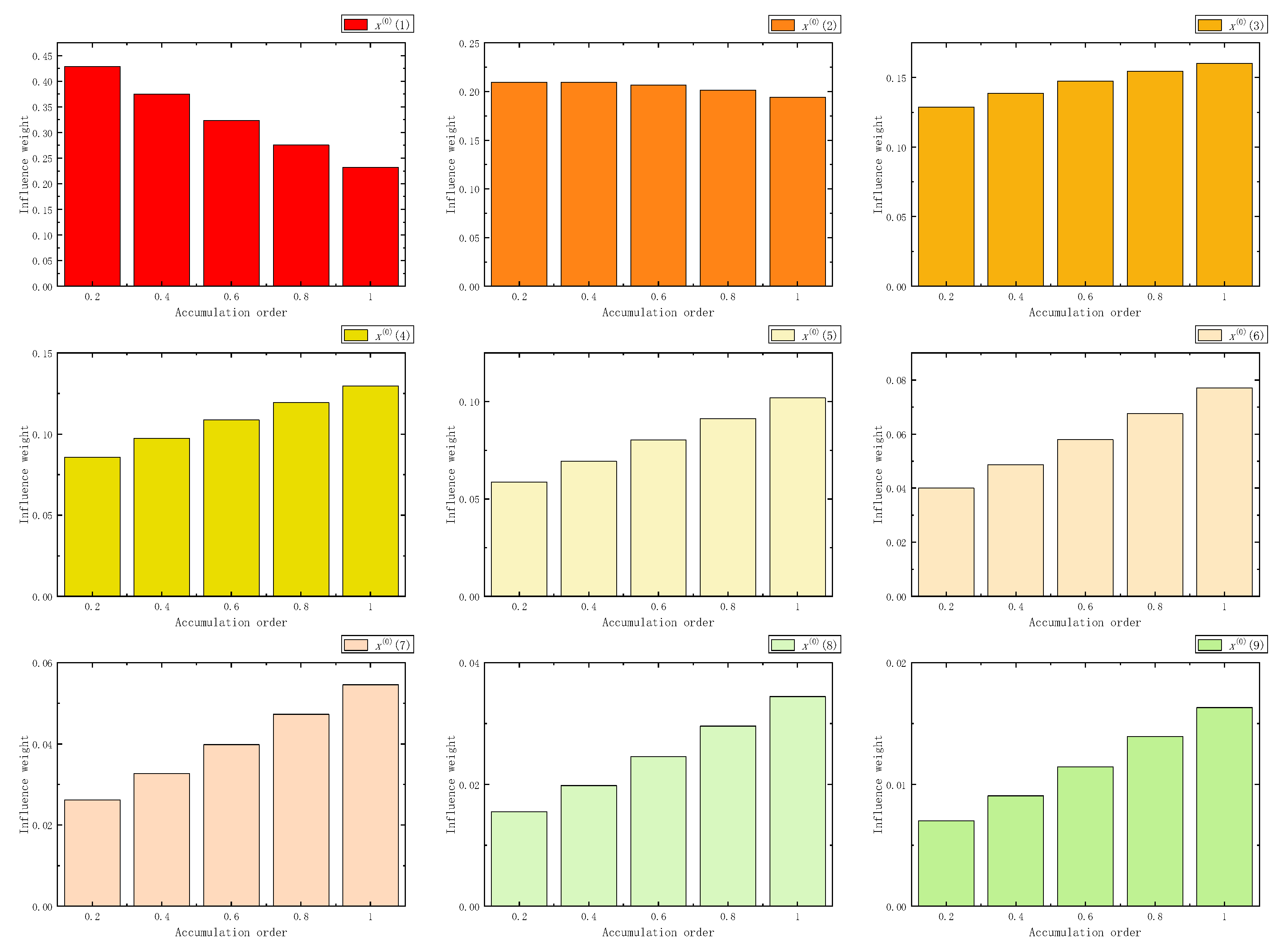
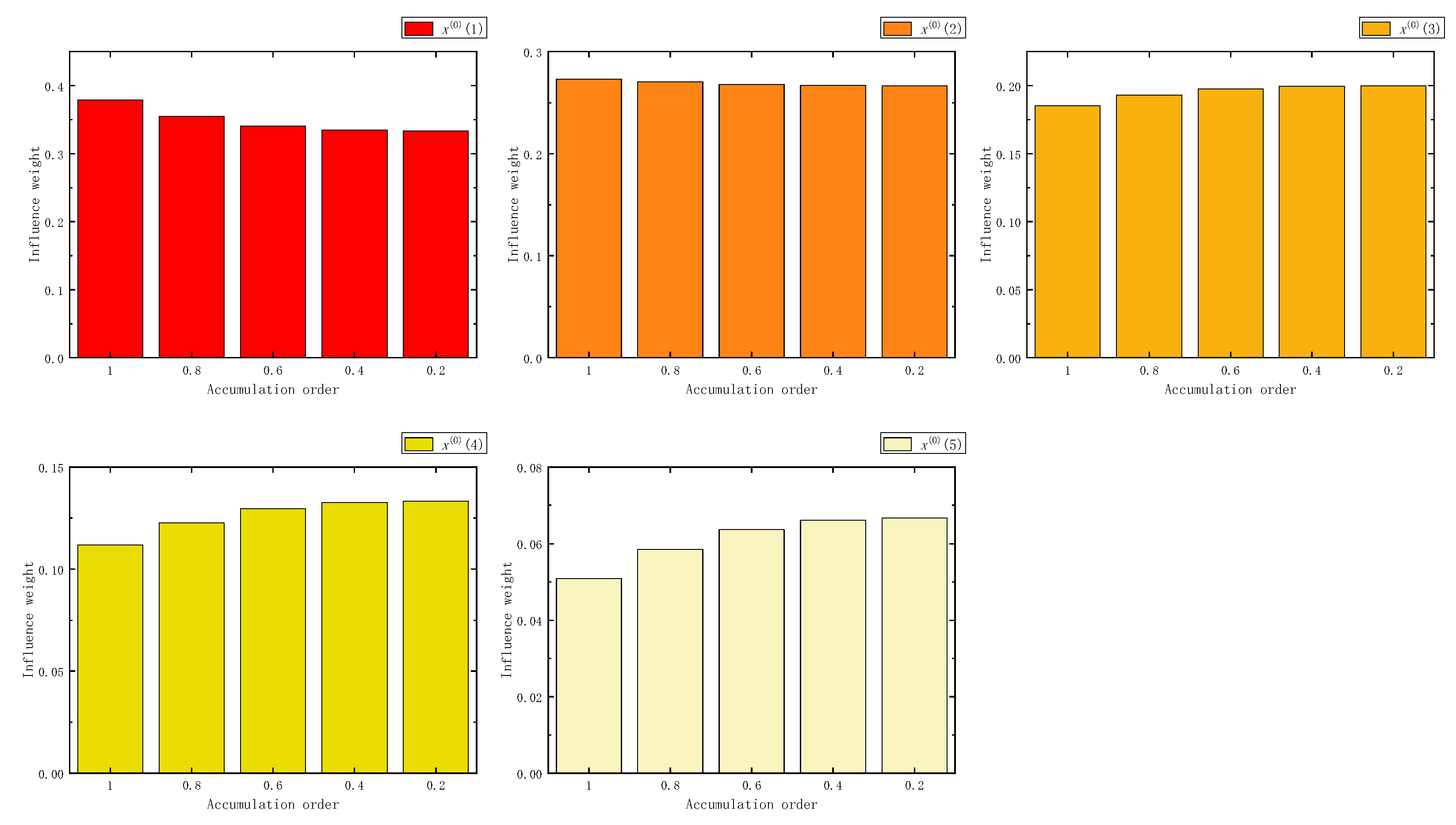
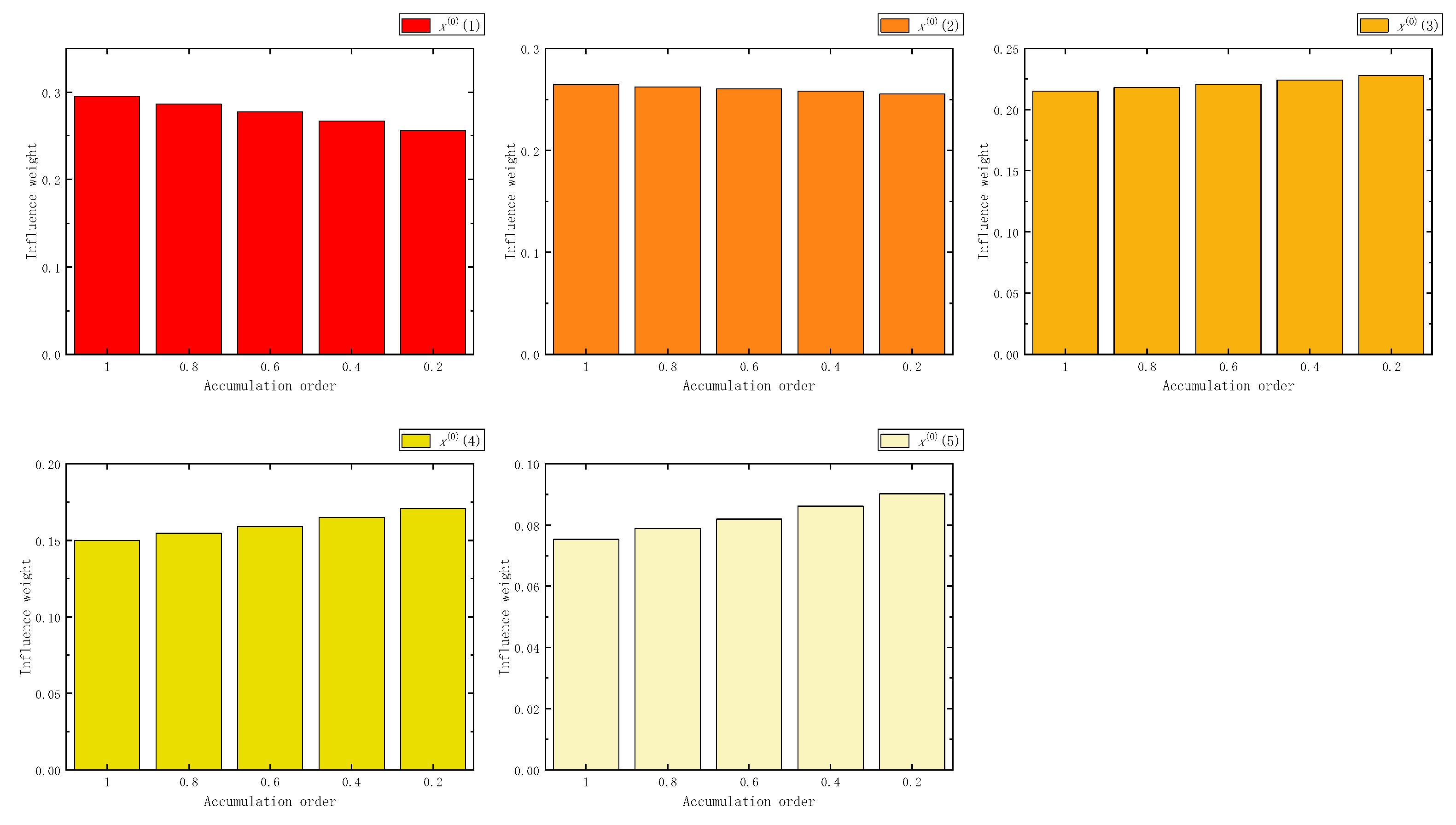
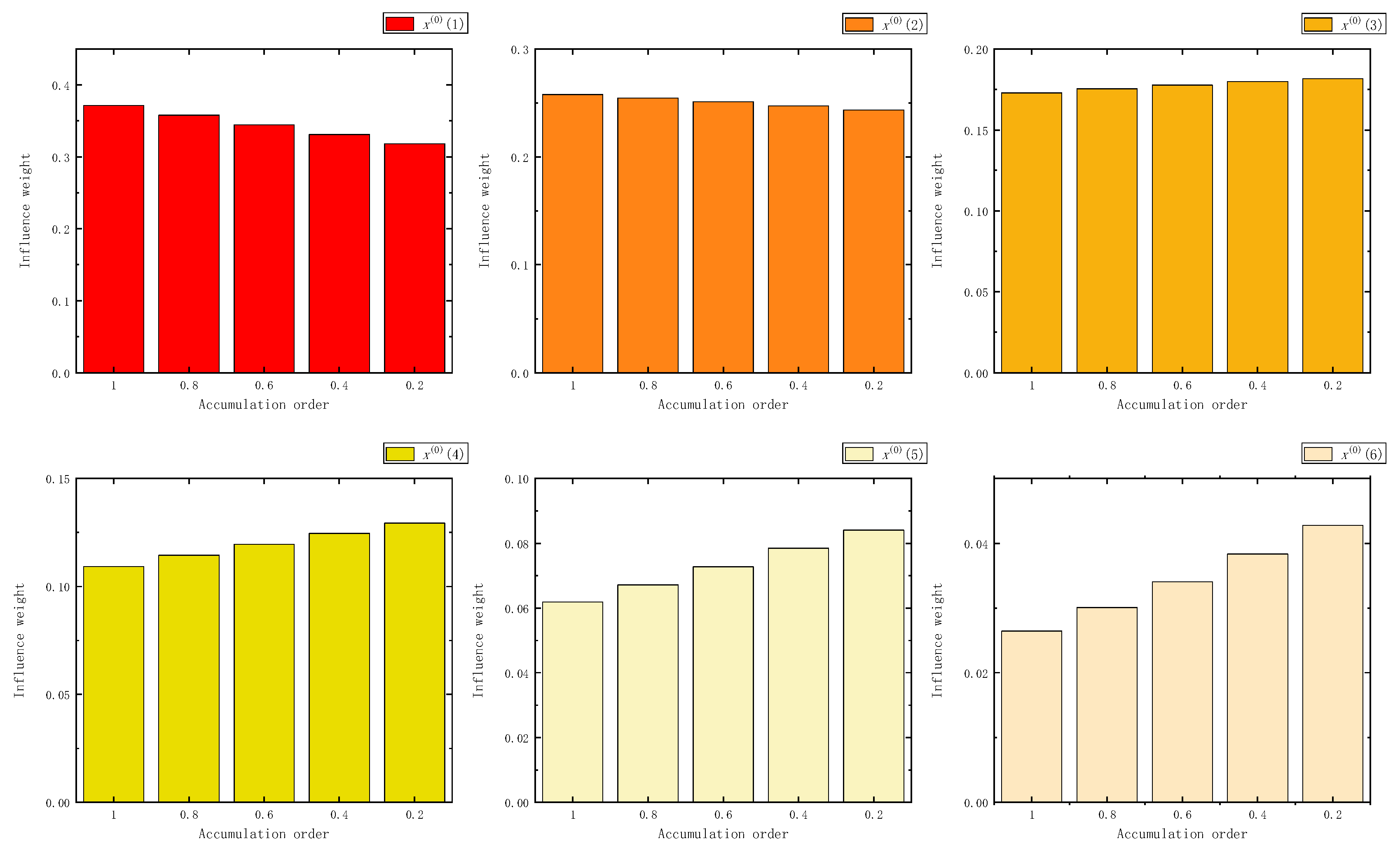
According to the FAGO in Equation (1), the variations in the influence degree of each sample under different accumulation orders are calculated, respectively. To further explore the influence degree of new and old information in the process of fractional order accumulation, the results were normalized. After the normalization process, the influence weight of the sample in FAGO is shown in Figure 2.

We can see that new information had the least influence weight, and old information had the greatest influence weight. Compared with the traditional first-order accumulation, in the sequence obtained by FAGO, as the accumulation order decreased, the influence weight of the new information increased, and the weight of the old information was reduced. New information always has a smaller influence than old information.

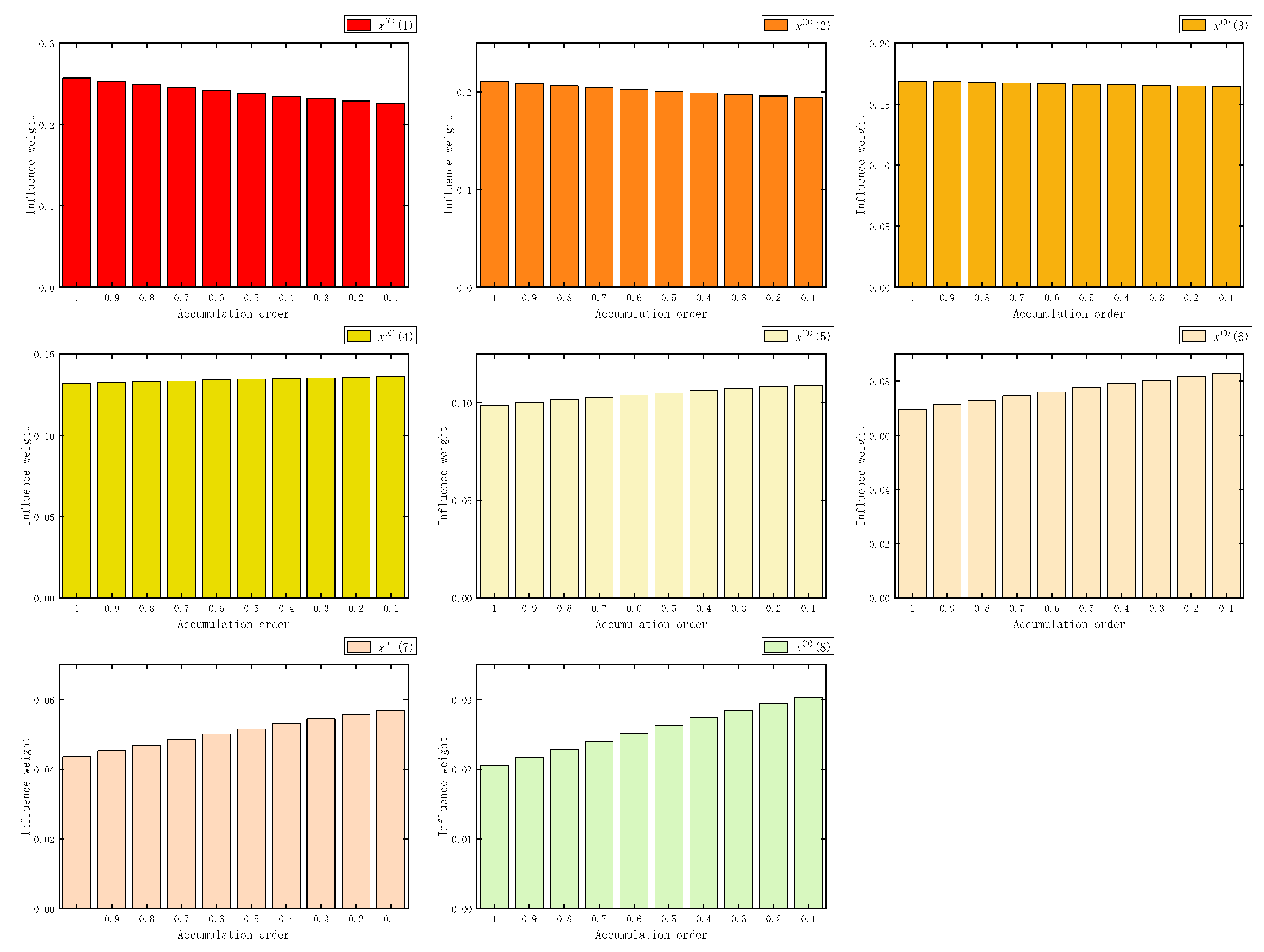
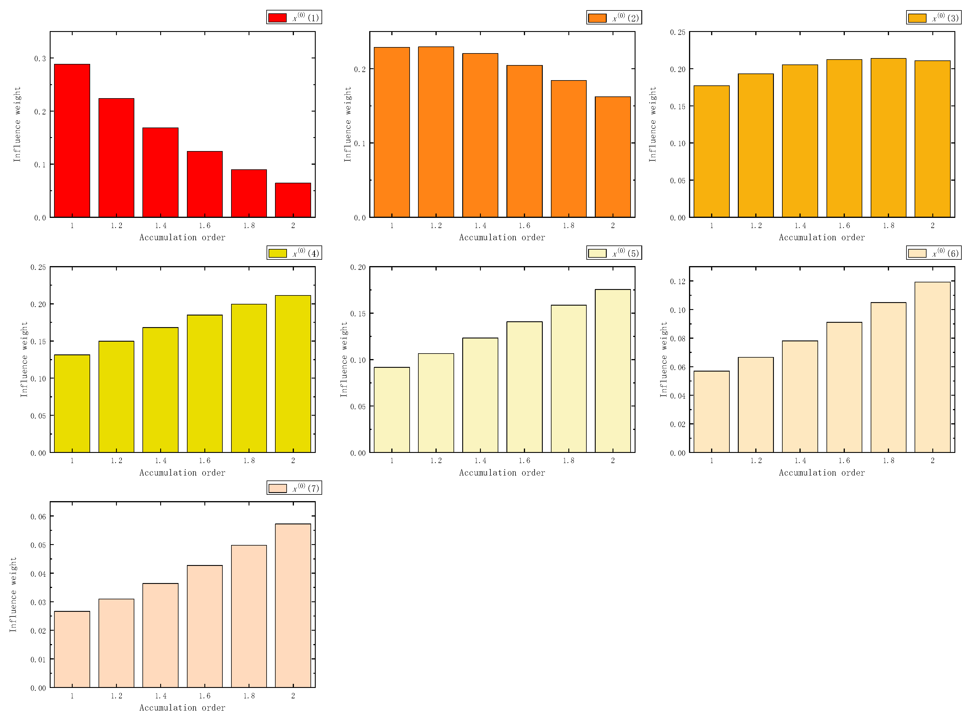
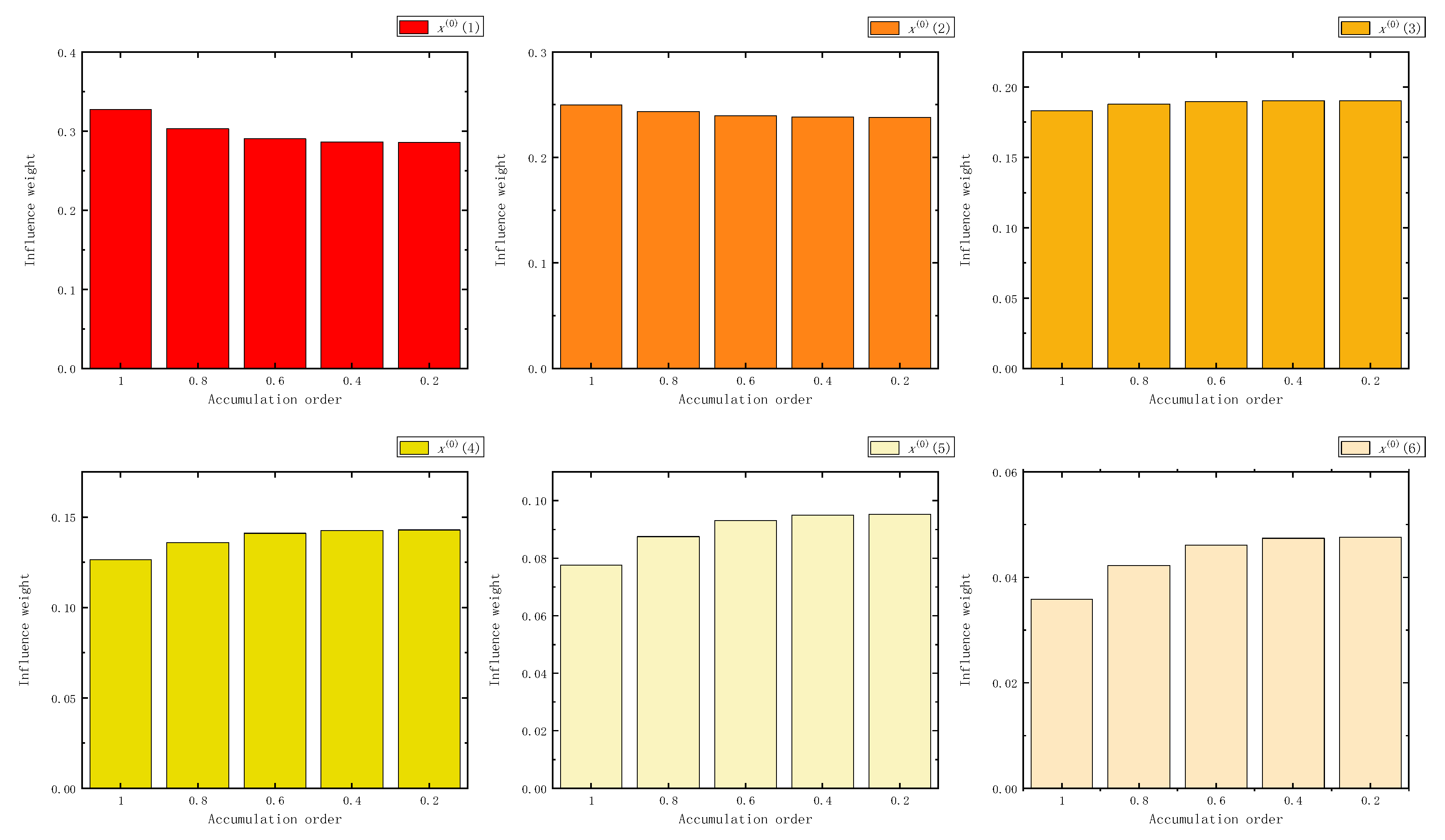
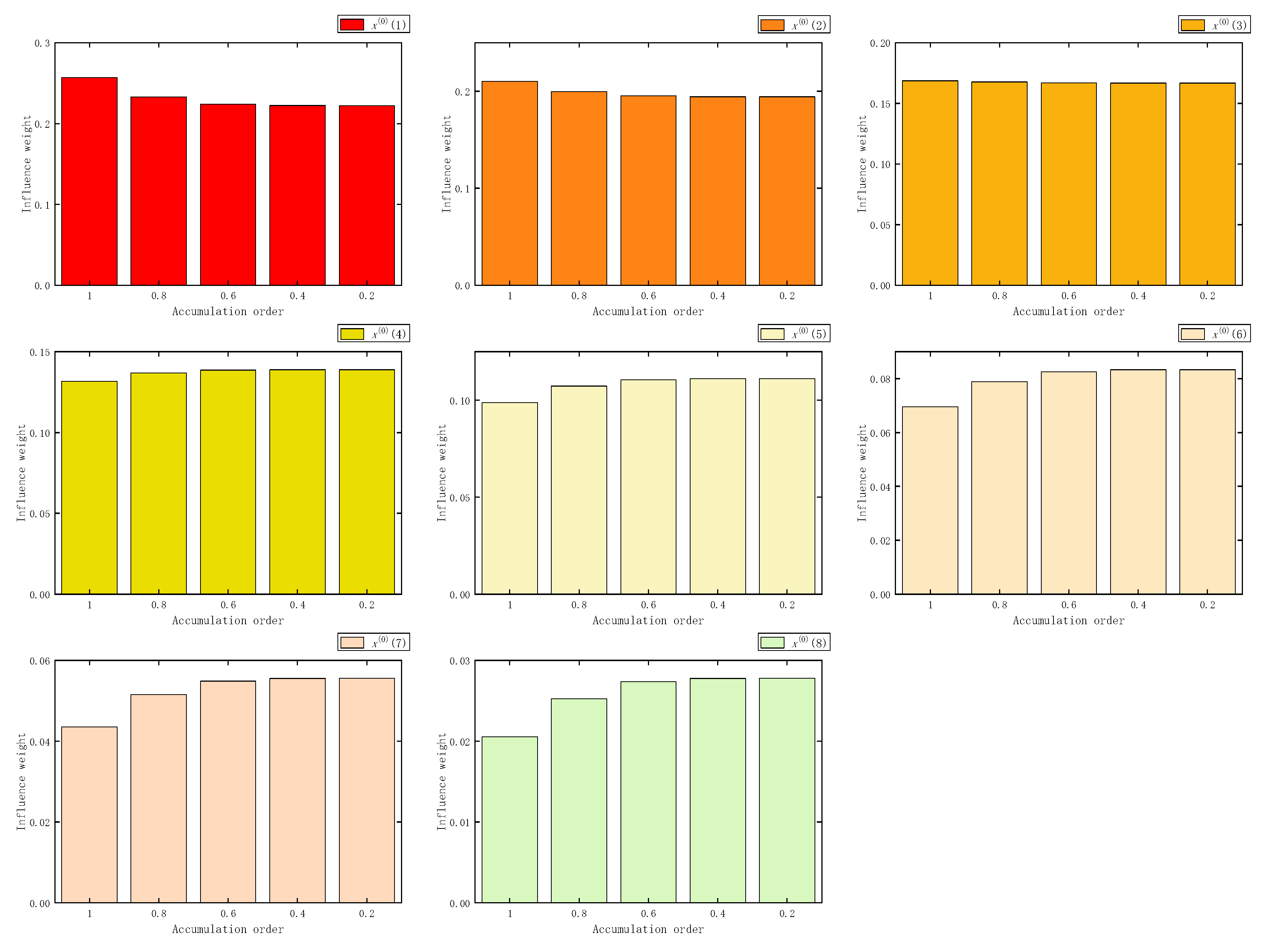
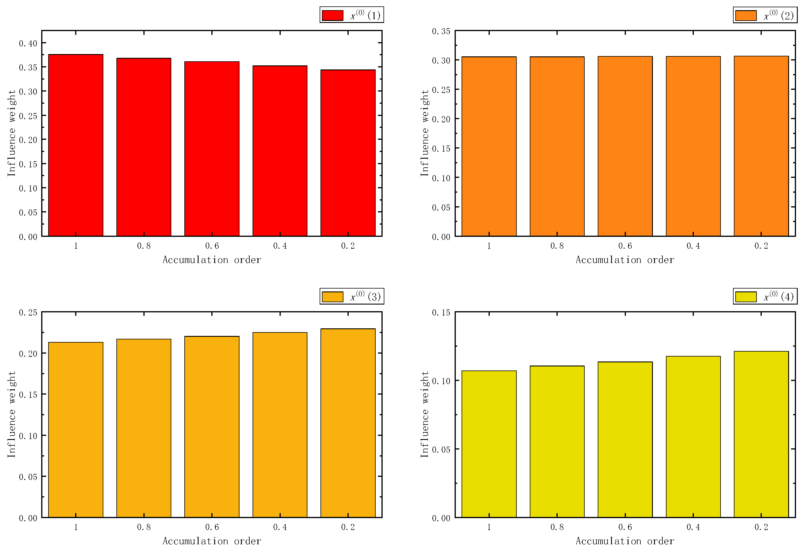
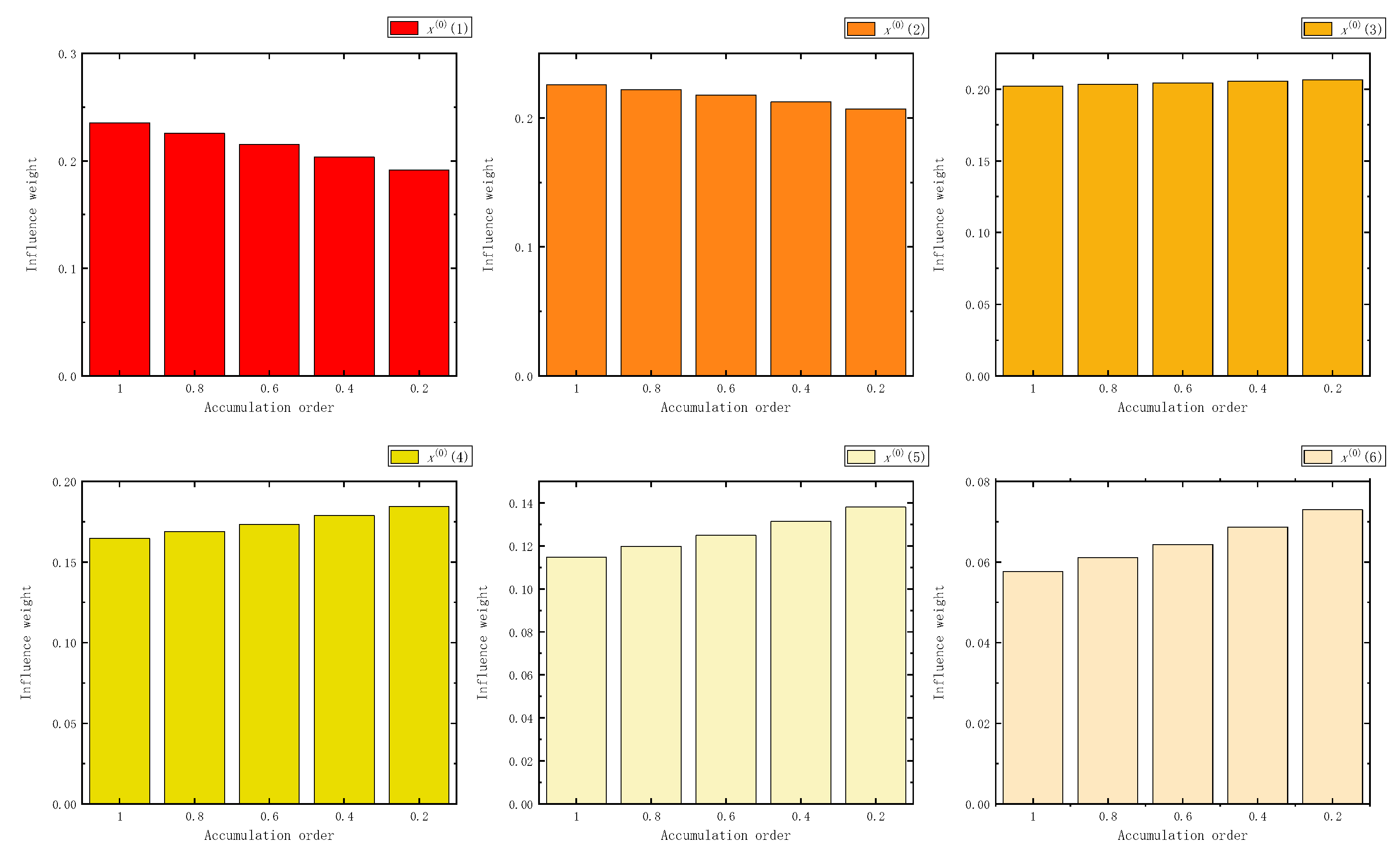
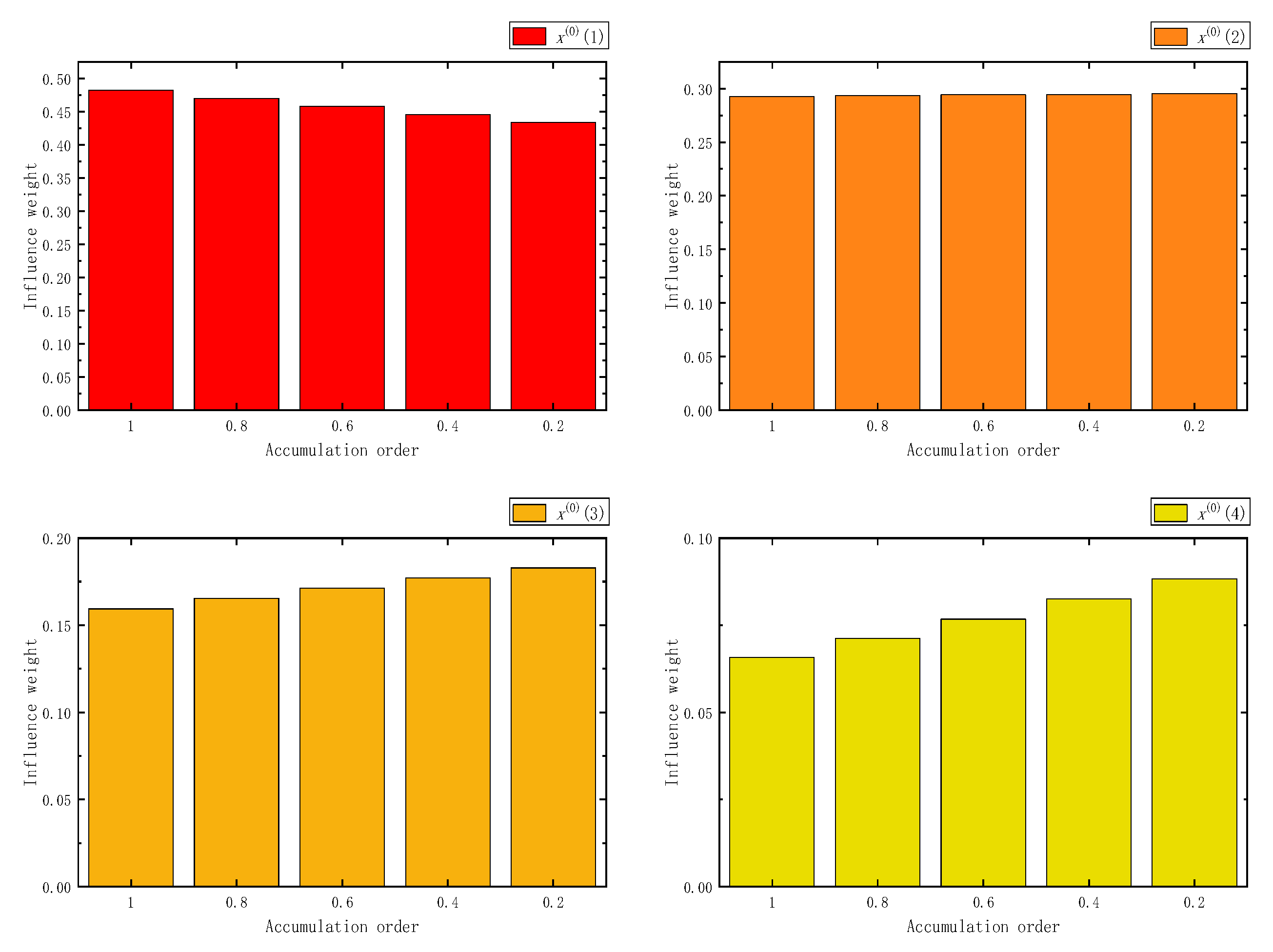
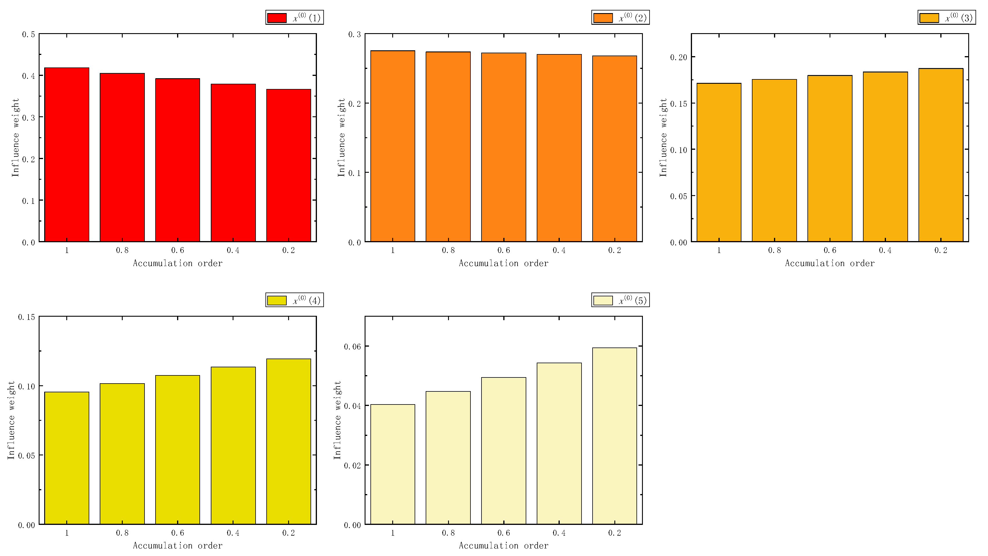
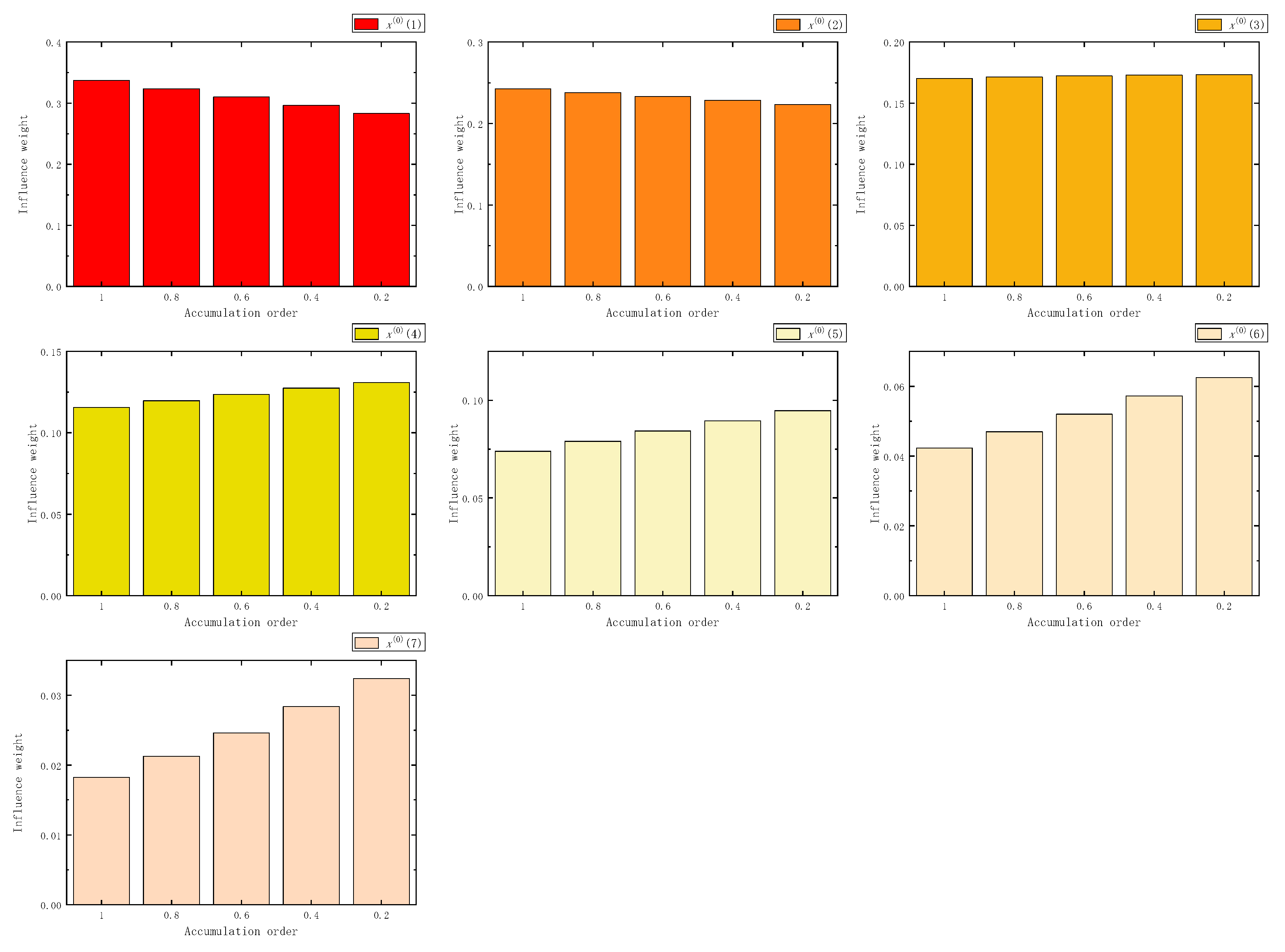
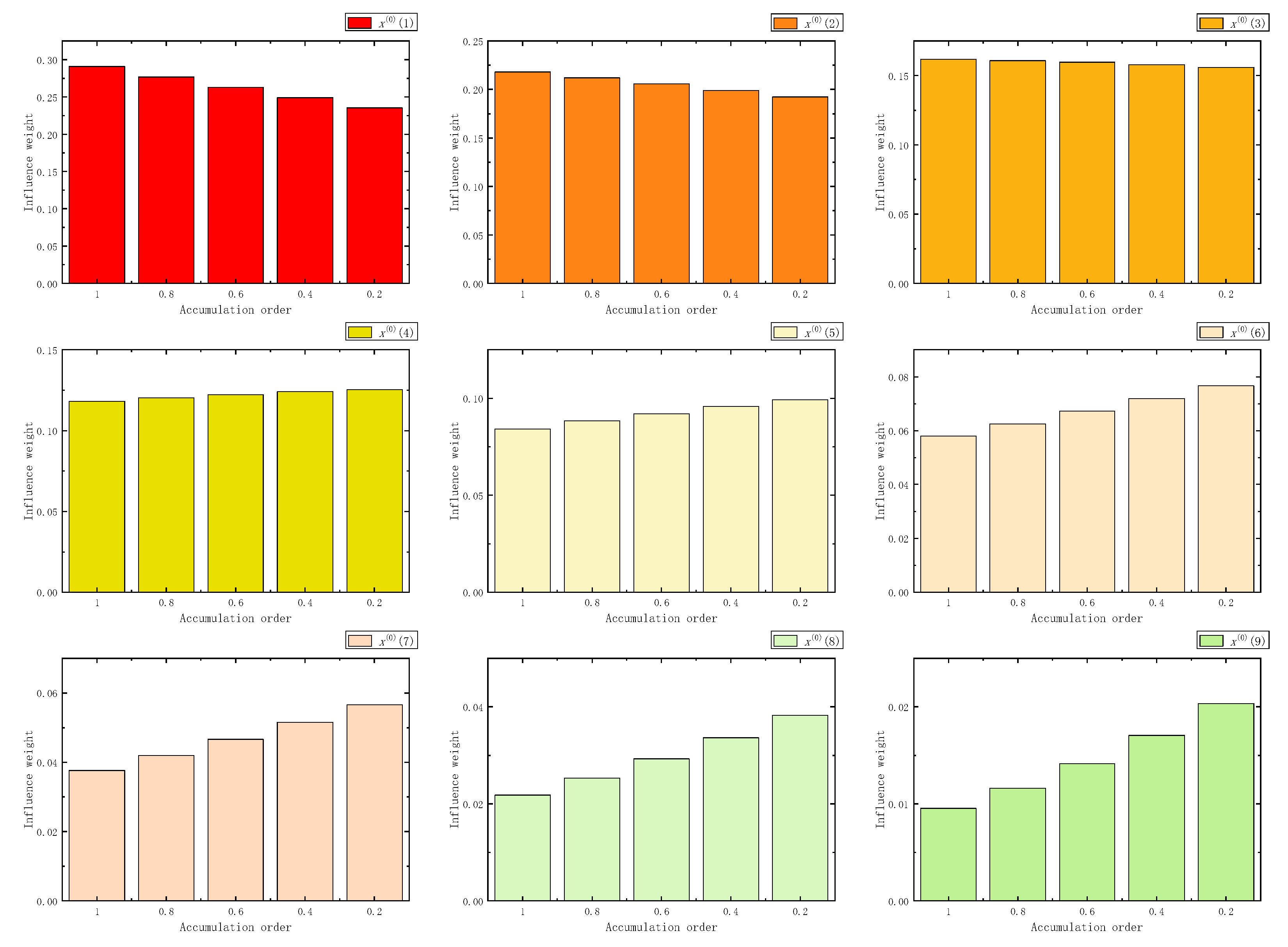
To verify whether the rule will fail due to the change in sample number, we calculated the variation of the influence weight with the accumulation order when the number of samples was 6 to 10, respectively, and the results are shown in Figure 3, Figure 4, Figure 5, Figure 6 and Figure 7.

Although the influence weight of each sample changed with the sample size, the above rules will not alter due to the increase in sample size. Therefore, it can be concluded that FAGO had an impact on the influence weight of new and old information. According to the above rules, the advantages of new information can be better utilized by changing the accumulation order.

3.2. The Impact of FHAGO on Different Sample Sizes

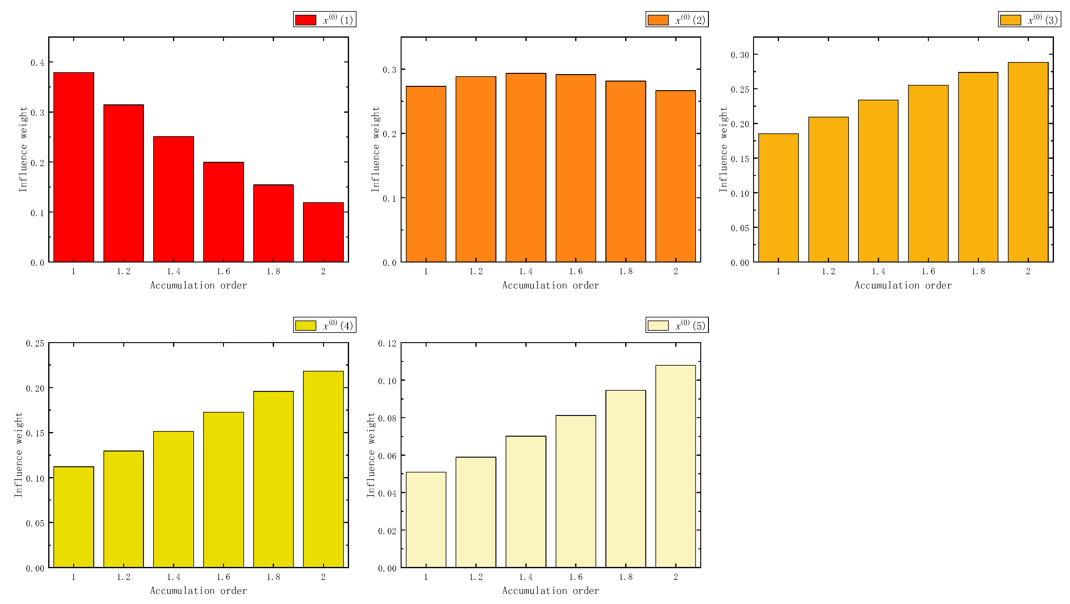
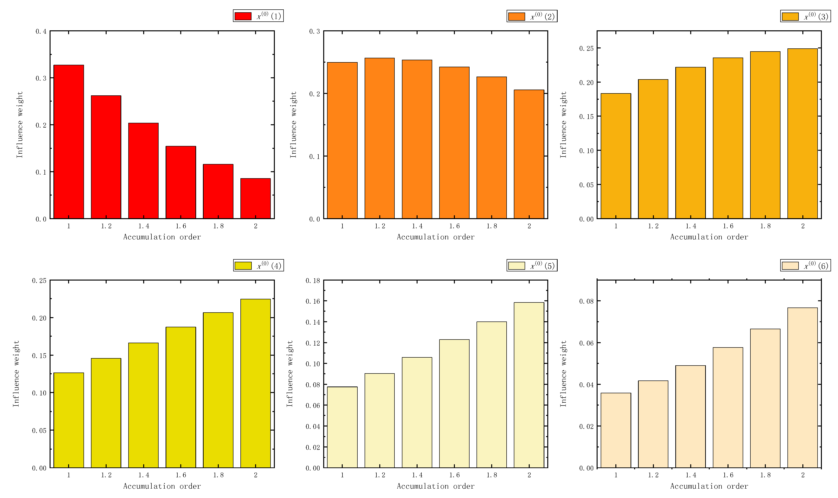
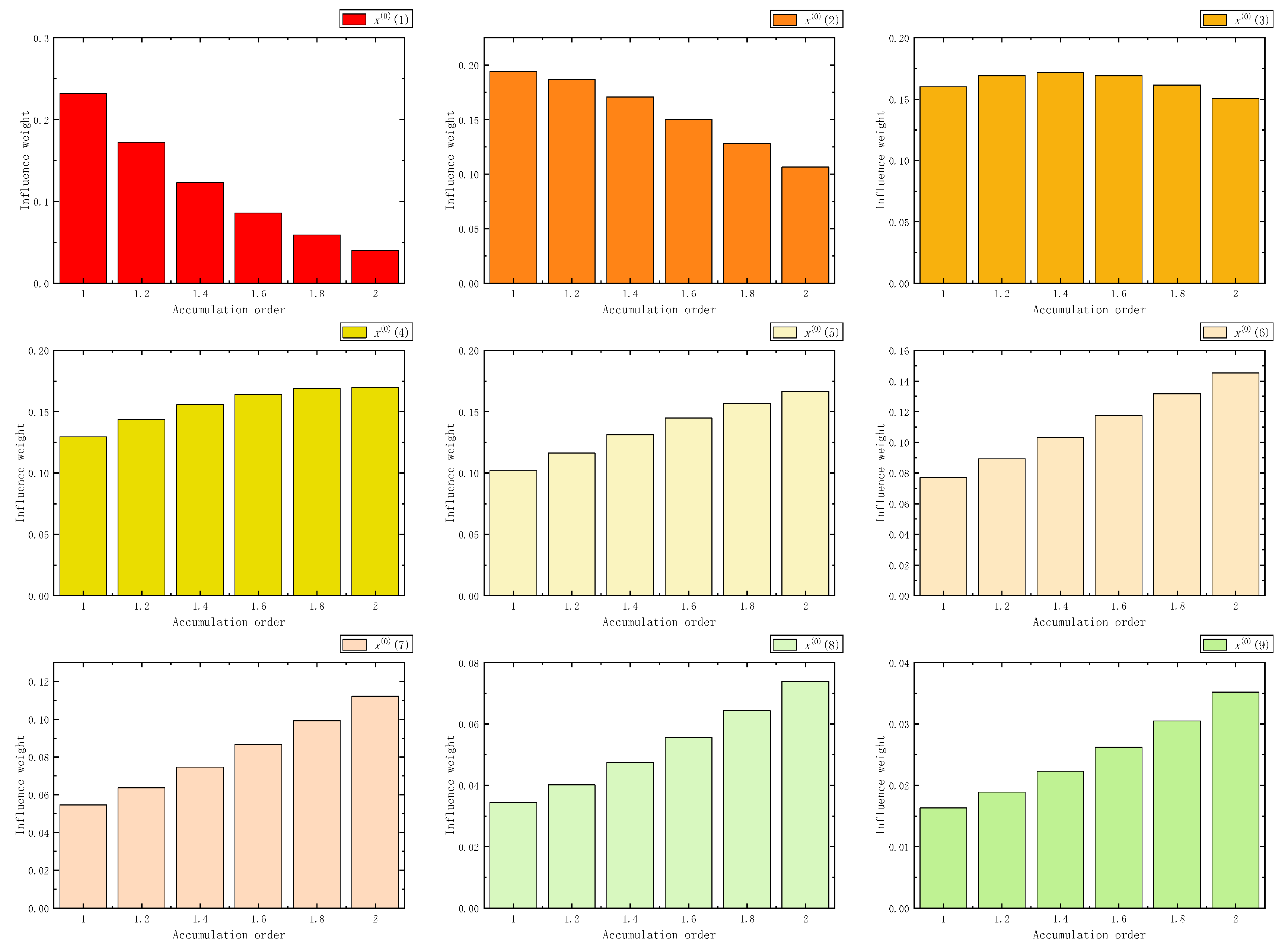
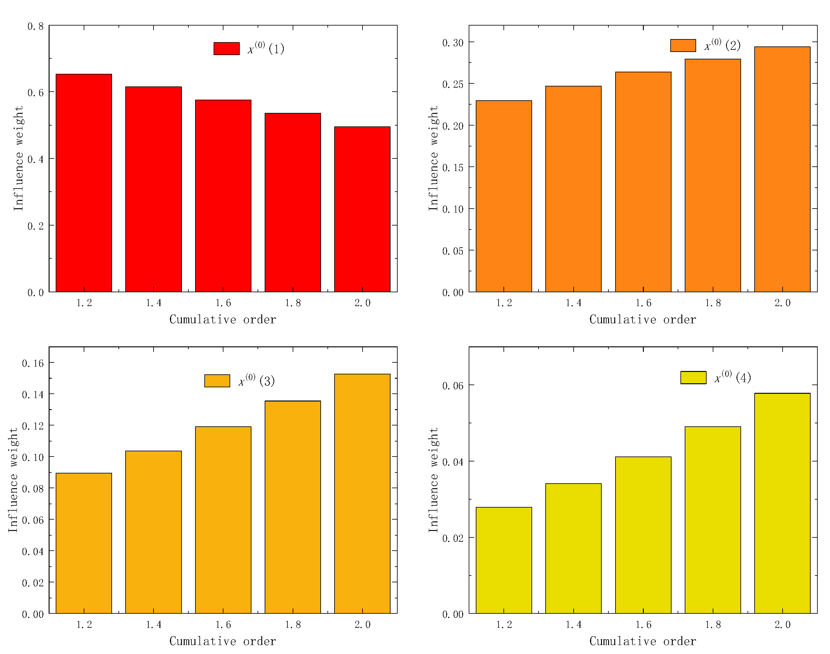
The results show that the restore error of the fractional Hausdorff grey model will be small when the order r > 1. Using the DEMATEL method to verify the influence of each sample in the model, the results are shown in Figure 8, Figure 9, Figure 10, Figure 11, Figure 12 and Figure 13.

As the accumulation order increased, the influence weight of new information showed an upward trend, and the influence weight of old information showed a downward trend, accordingly. In addition, when the sample size changed, the influence weight of each sample also changed accordingly, and the above rules did not alter due to the increase in sample size. Therefore, it can be concluded that FHAGO had an impact on the influence weight of the new and old information.

3.3. The Impact of CFAGO on Different Sample Sizes

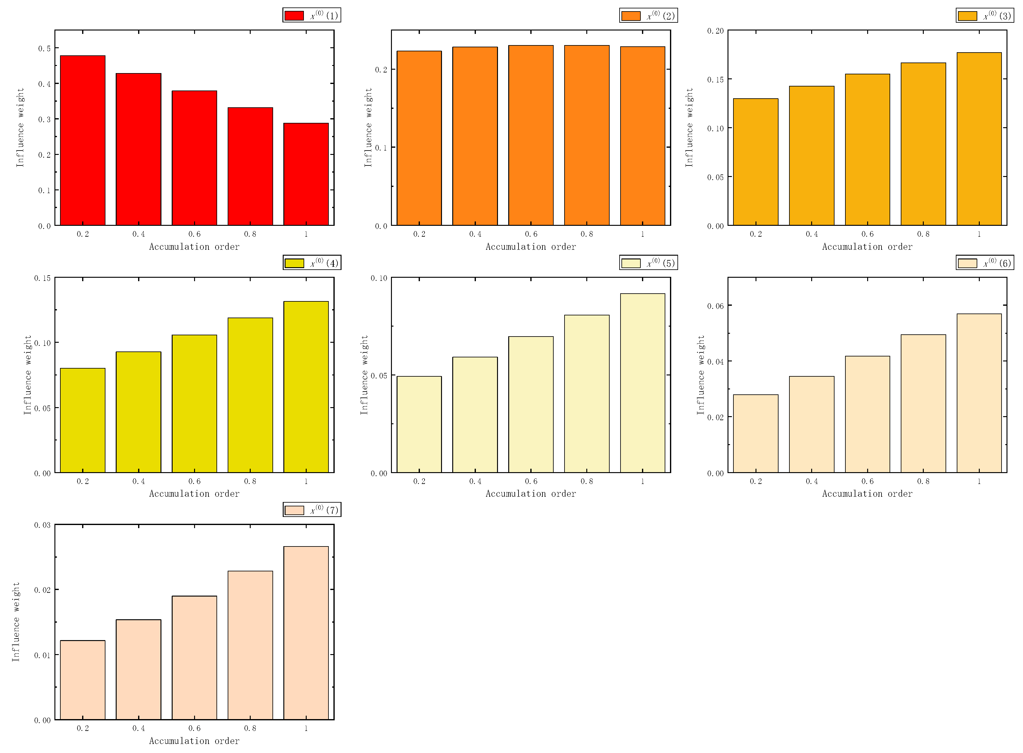
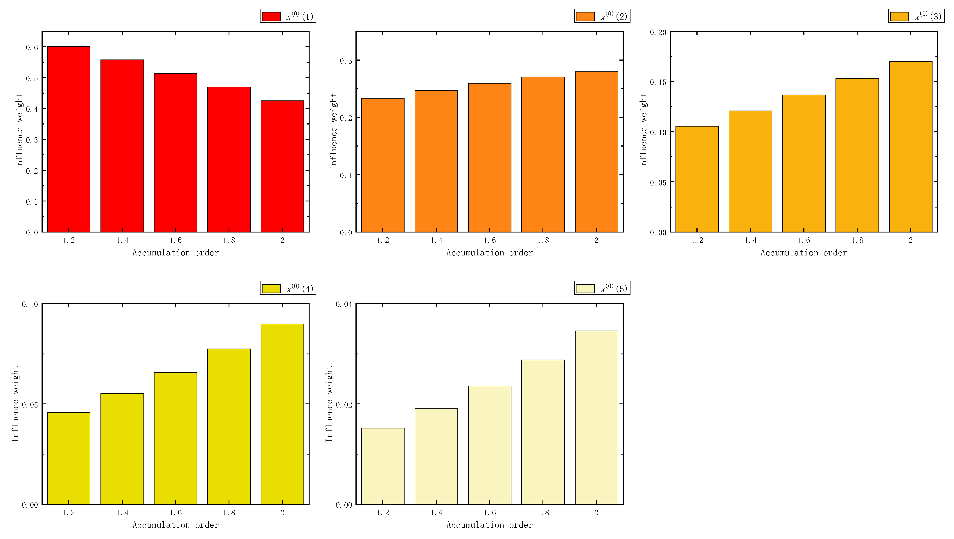
Since the range of accumulation order will cause different accumulation coefficients, we discuss the two cases of $0<r\le 1$ and $r>1$, respectively. When $0<r\le 1$, using the DEMATEL method to verify the influence of each sample in the model, the results are shown in Figure 14, Figure 15, Figure 16, Figure 17, Figure 18 and Figure 19.

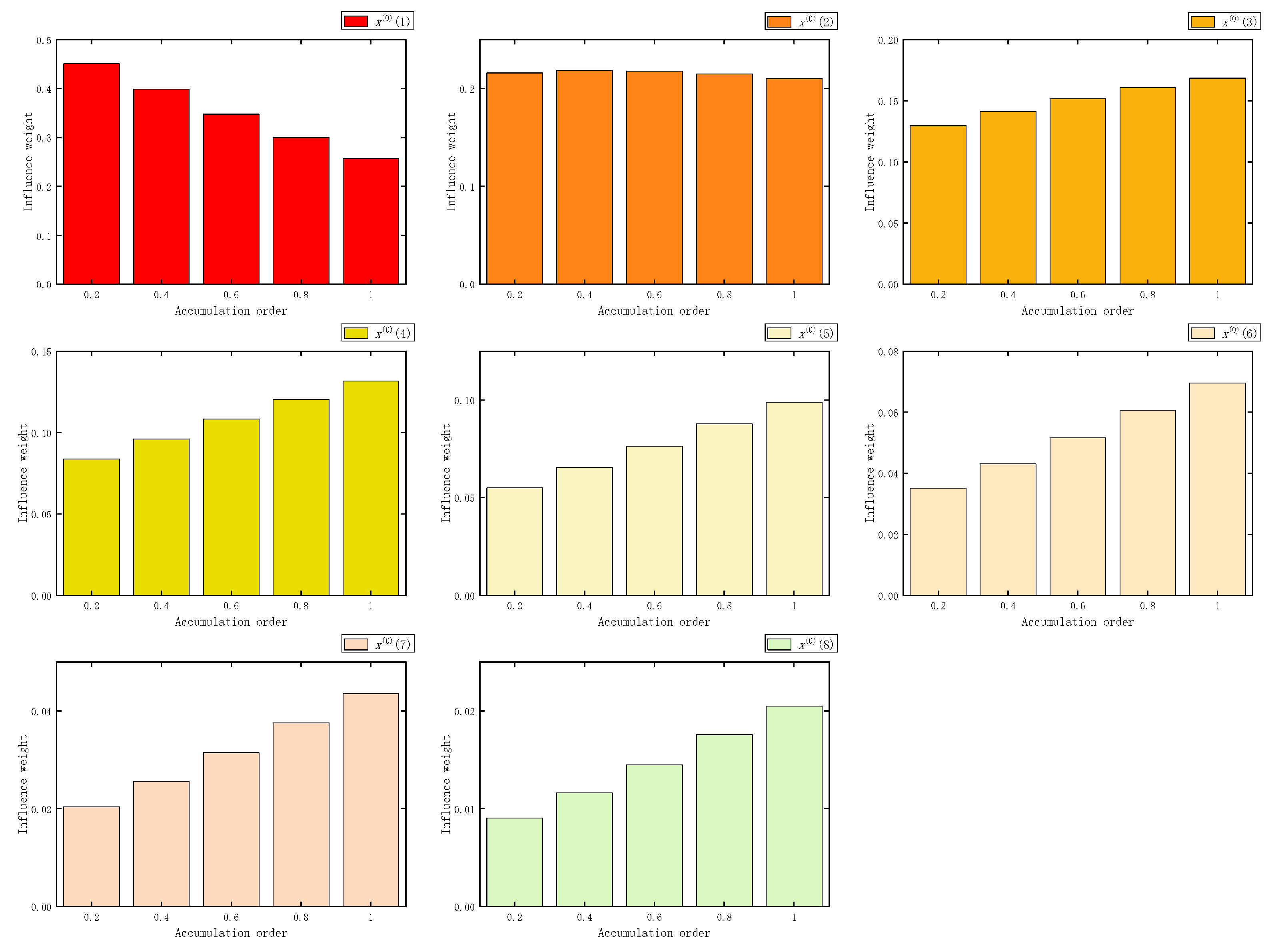
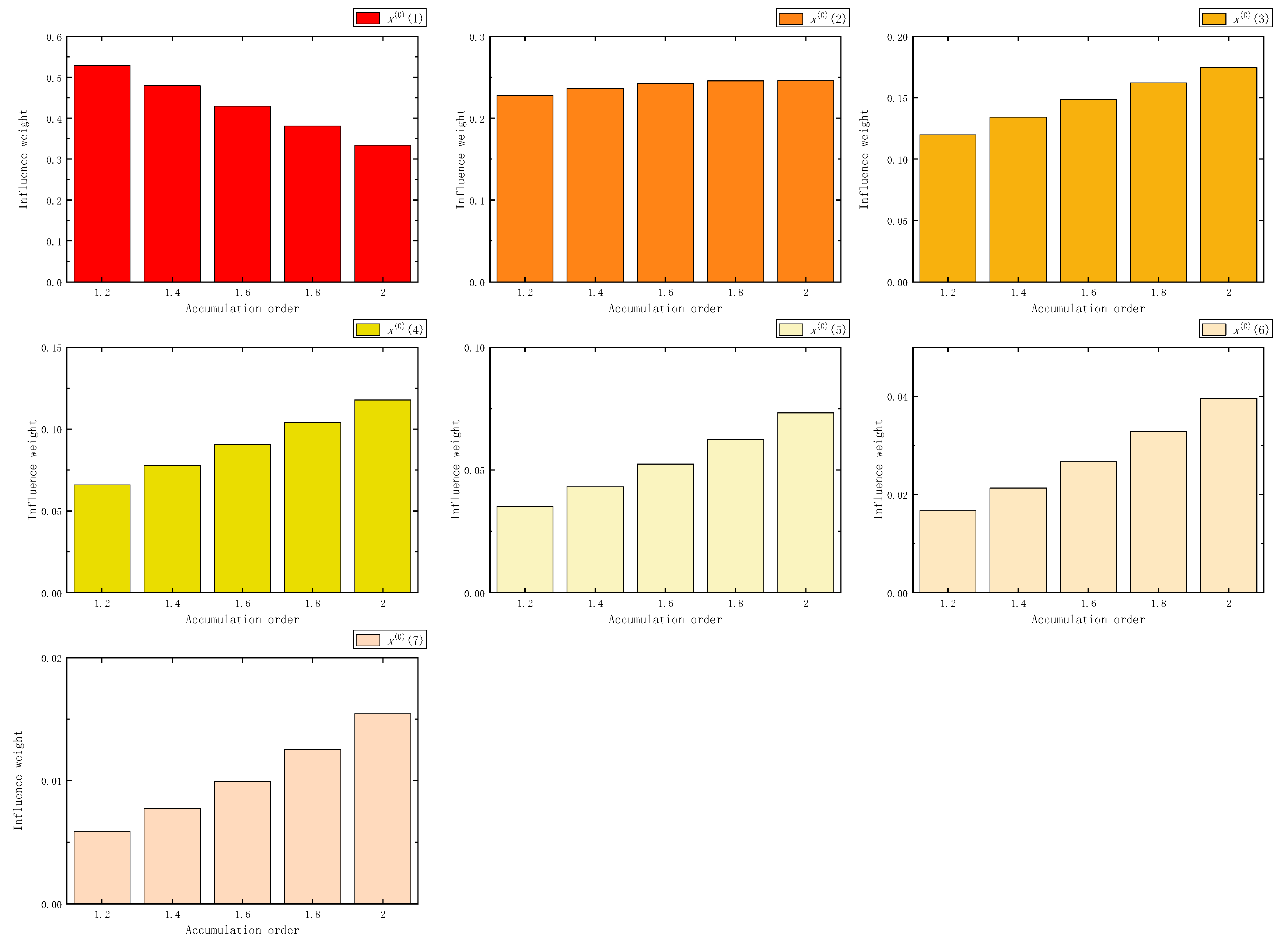
As can be seen from Figure 14, Figure 15, Figure 16, Figure 17, Figure 18 and Figure 19, when $0<r\le 1$, the influence weight of new information showed an upward trend with the accumulation order increasing, and the influence weight of old information accordingly showed a downward trend. When $r>1$, using the DEMATEL method to verify the influence of each sample in the model, the results are shown in Figure 20, Figure 21, Figure 22, Figure 23, Figure 24 and Figure 25.

From Figure 14, Figure 15, Figure 16, Figure 17, Figure 18, Figure 19, Figure 20, Figure 21, Figure 22, Figure 23, Figure 24 and Figure 25, the change in influence weight when $r>1$ was the same as that when $0<r\le 1$. The influence weight of new information showed an upward trend with the accumulation order increasing, and the influence weight of old information accordingly showed a downward trend.

In addition, when the sample size changed, the influence weight of each sample also changed accordingly, and the above rules did not alter due to the increase in sample size. Therefore, it can be concluded that CFAGO has an impact on the influence weight of the new and old information.

3.4. The Impact of NIPAGO on Different Sample Sizes

Using the DEMATEL method to verify the influence of each sample in the model, the results are shown in Figure 26, Figure 27, Figure 28, Figure 29, Figure 30 and Figure 31.

When $0.5<r<1$, the influence weight of new information increased as the accumulation order decreased, and the influence weight of old information decreased accordingly. Compared with the previous model, the change range of the influence weight of NIPAGO samples was relatively small, and after reaching a certain value, it would no longer change with the accumulation order dropping. In addition, when the sample size changed, the influence weight of each sample also changed accordingly, and the above rules would not alter due to the increase in sample size.

3.5. The Impact of DAGO on Different Sample Sizes

Using the DEMATEL method to verify the influence of each sample in the model, the results are shown in Figure 32, Figure 33, Figure 34, Figure 35, Figure 36 and Figure 37.

The influence weight of new information increased as the accumulation order decreased, and the influence weight of old information decreased accordingly. Moreover, when the sample size changed, the influence weight of each sample also changed accordingly, and the above rules would not alter due to the increase in sample size.

3.6. The Impact of WFAGO on Different Sample Sizes

Using the DEMATEL method to verify the influence of each sample in the model, the results are shown in Figure 38, Figure 39, Figure 40, Figure 41, Figure 42 and Figure 43.

Parallel to the 1-AGO, FAGO, NIPAGO, and DAGO, the influence weight in the calculation process of the WFAGO conformed to the variation regularity of all previous AGOs. When 0 < r ≤ 1, the influence weight of new information increased with the reduction of r, and the influence weight of old information decreased with the reduction of r. The rest of the parameters in the combined model except r also had an impact on the influence weight of old and new information, which will not be repeated here.

3.7. Summary of Influence Degree under Different AGOs

Based on the above results, it can be observed that the sample size did not affect the pattern of the influence degree with respect to the order. According to the principle of new information priority, our objective was to maximize the utilization of new information. In other words, we wanted to minimize the influence degree of old information and maximize the influence degree of new information. The influence degree regularity under different AGOs is shown in

Table 9. Influence degree regularity under different AGOs.

AGOs	Accumulation Order	Influence Degree
		New Information	Old Information
1-AGO	Fixed	Fixed	Fixed
FAGO	Decreasing	Increasing	Decreasing
FHAGO	Increasing	Significantly increasing	Significantly decreasing
CFAGO	Increasing	Significantly increasing	Significantly decreasing
NIPAGO	Decreasing	Increasing	Decreasing
DAGO	Decreasing	Significantly increasing	Significantly decreasing
WFAGO	Decreasing	Increasing	Decreasing

.

The 1-AGO could not be adjusted, resulting in a fixed influence degree for both old and new information. Nevertheless, the FAGO and other AGOs allowed the influence degree to vary with the accumulation order. In FAGO, NIPAGO, DAGO, and WFAGO, the influence degree of new information significantly increased as the accumulation order decreased. In CFAGO, the influence weight of new information showed an upward trend with an increase in the accumulation order. FHAGO exhibited the largest increase when r > 1. Accordingly, in FAGO, NIPAGO, DAGO, and WFAGO, a smaller accumulation order resulted in a higher influence degree of new information. Conversely, a larger accumulation order in FHAGO and CFAGO led to a higher influence degree of new information. This may enable researchers to select a more appropriate accumulation order that aligns with the principle of new information priority.

4. Conclusions

In this paper, we have summarized different AGOs in grey system models and revealed the relationships and influences among them based on the DEMATEL method. Subsequently, the variation regularity of the influence degree on separate accumulation orders in each AGO was obtained. Based on the calculation and analysis, the following conclusions can be drawn.

• Compared with the traditional 1-AGO, the FAGO, FHAGO, CFAGO, NIPAGO, DAGO, and WFAGO can change the influence degree of new and old information to sufficiently utilize the data advantages of new information.
• Different accumulation methods have different effects on new and old information, i.e., FAGO, NIPAGO, DAGO, and WFAGO make the influence degree of new information show an upward trend with a reduction in the accumulation order, while FHAGO and CFAGO make the influence degree of new information increase with the acceleration of the accumulation order. Furthermore, this rule does not fail with the variation of the sample size.

According to the above rules, the advantages of new information can be better utilized by changing the accumulation order. It can provide some reference for the selection of the accumulation orders of various grey forecasting models. Future research will further expand the application scope of this method. It can delve deeper into exploring the potential application of DEMATEL in other models, such as assessing the impact of new and old information in the metabolic grey model to determine whether it has a new information priority. Additionally, it can also combine other evaluation indicators for comprehensive analysis to investigate the utilization of information under different AGOs.

References

1. Johannesen, N.J.; Kolhe, M.; Goodwin, M. Relative Evaluation of Regression Tools for Urban Area Electrical Energy Demand Forecasting. J. Clean. Prod. 2019, 218, 555–564. [Google Scholar] [CrossRef]
2. Cabaneros, S.M.; Calautit, J.K.; Hughes, B.R. A Review of Artificial Neural Network Models for Ambient Air Pollution Prediction. Environ. Modell. Softw. 2019, 119, 285–304. [Google Scholar] [CrossRef]
3. He, J.; Mao, S.; Kang, Y. Augmented Fractional Accumulation Grey Model and Its Application: Class Ratio and Restore Error Perspectives. Math. Comput. Simul. 2023, 209, 220–247. [Google Scholar] [CrossRef]
4. Singh, P.K.; Pandey, A.K.; Bose, S.C. A New Grey System Approach to Forecast Closing Price of Bitcoin, Bionic, Cardano, Dogecoin, Ethereum, XRP Cryptocurrencies. Qual. Quant. 2023, 57, 2429–2446. [Google Scholar] [CrossRef]
5. Duan, H.; Liu, Y.; Wang, G. A Novel Dynamic Time-Delay Grey Model of Energy Prices and Its Application in Crude Oil Price Forecasting. Energy 2022, 251, 123968. [Google Scholar] [CrossRef]
6. Li, Q.; Wang, Z.-X.; Zhang, X.-Y. An Improved Gray Bernoulli Model for Estimating the Relationship between Economic Growth and Pollution Emissions. Environ. Sci. Pollut. R. 2020, 27, 25638–25654. [Google Scholar] [CrossRef]
7. Zhang, Z.; Wu, L.; Chen, Y. Forecasting PM2.5 and PM10 Concentrations Using GMCN(1,N) Model with the Similar Meteorological Condition: Case of Shijiazhuang in China. Ecol. Indic. 2020, 119, 106871. [Google Scholar] [CrossRef]
8. Manivanna Boopathi, A.; Mohamed Ali, E.A.; Subha, V.; Abudhahir, A. Forecasting the Generation and Consumption of Electricity and Water in Kingdom of Bahrain Using Grey Models. Int. J. Comput. Digit. Syst. 2021, 10, 1–8. [Google Scholar] [CrossRef]
9. Şahin, U. Future of Renewable Energy Consumption in France, Germany, Italy, Spain, Turkey and UK by 2030 Using Optimized Fractional Nonlinear Grey Bernoulli Model. Sustain. Prod. Consum. 2021, 25, 1–14. [Google Scholar] [CrossRef] [PubMed]
10. Deng, J.L. Control Problems of Grey Systems. Syst. Control Lett. 1982, 1, 288–294. [Google Scholar] [CrossRef]
11. Getanda, V.B.; Kihato, P.K.; Hinga, P.K.; Oya, H. Data Grouping and Modified Initial Condition in Grey Model Improvement for Short-Term Traffic Flow Forecasting. Automatika 2022, 64, 178–188. [Google Scholar] [CrossRef]
12. Madhi, M.H.; Mohamed, N. An Improved GM(1,1) Model Based on Modified Background Value. Inf. Technol. J. 2017, 16, 11–16. [Google Scholar] [CrossRef]
13. Cao, C.; Fan, C.; Hu, Z. Grey Forecasting Model and Its Application Based on the Sine Function Transformation. J. Math. 2013, 33, 697–701. [Google Scholar] [CrossRef]
14. Nguyen, N.T.; Phan, V.T.; Malara, Z. Nonlinear Grey Bernoulli Model Based on Fourier Transformation and Its Application in Forecasting the Electricity Consumption in Vietnam. J. Intell. Fuzzy Syst. 2019, 37, 7631–7641. [Google Scholar] [CrossRef]
15. Zhou, D.; AlDurra, A.; Zhang, K.; Ravey, A.; Gao, F. A Robust Prognostic Indicator for Renewable Energy Technologies: A Novel Error Correction Grey Prediction Model. IEEE Trans. Ind. Electron. 2019, 66, 9312–9325. [Google Scholar] [CrossRef]
16. Rajesh, R.; Agariya, A.K.; Rajendran, C. Predicting Resilience in Retailing Using Grey Theory and Moving Probability Based Markov Models. J. Retail. Consum. Serv. 2021, 62, 102599. [Google Scholar] [CrossRef]
17. Wu, L.F.; Liu, S.F.; Yao, L.G.; Yan, S.L.; Liu, D.L. Grey System Model with the Fractional Order Accumulation. Commun. Nonlinear Sci. Numer. Simul. 2013, 18, 1775–1785. [Google Scholar] [CrossRef]
18. Gao, M.; Yang, H.; Xiao, Q.; Goh, M. A Novel Fractional Grey Riccati Model for Carbon Emission Prediction. J. Clean. Prod. 2021, 282, 124471. [Google Scholar] [CrossRef]
19. Zhao, H.; Wu, L. Forecasting the Non-Renewable Energy Consumption by an Adjacent Accumulation Grey Model. J. Clean. Prod. 2020, 275, 124113. [Google Scholar] [CrossRef]
20. Wu, L.F.; Zhao, H.Y. Discrete Grey Model with the Weighted Accumulation. Soft Comput. 2019, 23, 12873–12881. [Google Scholar] [CrossRef]
21. Wu, L.F.; Liu, S.F.; Fang, Z.G.; Xu, H.Y. Properties of the GM(1,1) with Fractional Order Accumulation. Appl. Math. Comput. 2015, 252, 287–293. [Google Scholar] [CrossRef]
22. Chen, Y.; Lifeng, W.; Lianyi, L.; Kai, Z. Fractional Hausdorff Grey Model and Its Properties. Chaos Solitons Fractals 2020, 138, 109915. [Google Scholar] [CrossRef]
23. Ma, X.; Wu, W.; Zeng, B.; Wang, Y.; Wu, X. The Conformable Fractional Grey System Model. ISA Trans. 2020, 96, 255–271. [Google Scholar] [CrossRef] [PubMed]
24. Zhou, W.J.; Zhang, H.R.; Dang, Y.G.; Wang, Z.X. The Construction and Application of the Grey Discrete Model of Innovation Priority Accumulation. Chin. J. Manag. Sci. 2017, 25, 140–148. [Google Scholar] [CrossRef]
25. Liu, L.; Chen, Y.; Wu, L. The Damping Accumulated Grey Model and Its Application. Commun. Nonlinear Sci. Numer. Simul. 2021, 95, 105665. [Google Scholar] [CrossRef]
26. Zhu, H.G.; Liu, C.; Wu, W.Z.; Xie, W.L.; Lao, T.F. Weakened Fractional-Order Accumulation Operator for Ill-Conditioned Discrete Grey System Models. Appl. Math. Model. 2022, 111, 349–362. [Google Scholar] [CrossRef]
27. Xiao, X.; Yang, J.; Mao, S.; Wen, J. An Improved Seasonal Rolling Grey Forecasting Model Using a Cycle Truncation Accumulated Generating Operation for Traffic Flow. Appl. Math. Model. 2017, 51, 386–404. [Google Scholar] [CrossRef]
28. Li, K.; Xiong, P.; Wu, Y.; Dong, Y. Forecasting Greenhouse Gas Emissions with the New Information Priority Generalized Accumulative Grey Model. Sci. Total Environ. 2022, 807, 150859. [Google Scholar] [CrossRef]
29. Guo, J.; Chen, Y.; Wu, L. Using the Quarterly Compound Fractional Grey Model to Predict the Air Quality in 22 Cities of China. J. Math. 2021, 2021, e4959457. [Google Scholar] [CrossRef]
30. Che, X.Y.; Luo, Y.X.; He, Z.M. Grey New Information GOM(1,1) Model Based on Opposite-Direction Accumulated Generating and Its Application. Appl. Mech. Mater. 2013, 364, 207–210. [Google Scholar] [CrossRef]
31. Si, S.; You, X.; Liu, H.; Zhang, P. DEMATEL Technique: A Systematic Review of the State-of-the-Art Literature on Methodologies and Applications. Math. Probl. Eng. 2018, 2018, e3696457. [Google Scholar] [CrossRef]
32. Thakkar, J.J. Decision-making trial and evaluation laboratory (DEMATEL). In Multi-Criteria Decision Making; Thakkar, J.J., Ed.; Studies in Systems, Decision and Control; Springer: Singapore, 2021; pp. 139–159. ISBN 978-981-334-745-8. [Google Scholar]
33. Liao, C. Applying the DEMATEL Method to Evaluate Social Media Criteria in Promoting Sustainable Health Behavior—A Case Study of Vegetarian Diet Promotion by a Non-Profit Organization. Sustainability 2022, 14, 16973. [Google Scholar] [CrossRef]
34. Shieh, J.; Wu, H.H.; Huang, K. A DEMATEL Method in Identifying Key Success Factors of Hospital Service Quality. Knowl. Based Syst. 2010, 23, 277–282. [Google Scholar] [CrossRef]
35. Zhang, W.; Deng, Y. Combining Conflicting Evidence Using the DEMATEL Method. Soft Comput. 2019, 23, 8207–8216. [Google Scholar] [CrossRef]
36. dos Santos Soares, T.; Silva, M.M.; Santos, S.M. A Hybrid Grey-DEMATEL Approach to Identify Barriers to the Implementation of an End-of-Life Vehicle Management System in Brazil. J. Clean. Prod. 2023, 386, 135791. [Google Scholar] [CrossRef]
37. Dubey, N.; Tanksale, A. A Study of Barriers for Adoption and Growth of Food Banks in India Using Hybrid DEMATEL and Analytic Network Process. Socio-Econ. Plan. Sci. 2022, 79, 101124. [Google Scholar] [CrossRef]
38. Li, H.; Wang, W.; Fan, L.; Li, Q.; Chen, X. A Novel Hybrid MCDM Model for Machine Tool Selection Using Fuzzy DEMATEL, Entropy Weighting and Later Defuzzification VIKOR. Appl. Soft Comput. 2020, 91, 106207. [Google Scholar] [CrossRef]
Figure 1. The relation between the 1-AGO and other AGOs.
Fractalfract 07 00626 g001
Figure 2. The influence weight of five samples in FAGO.
Fractalfract 07 00626 g002
Figure 3. The influence weight of six samples in FAGO.
Fractalfract 07 00626 g003
Figure 4. The influence weight of seven samples in FAGO.
Fractalfract 07 00626 g004
Figure 5. The influence weight of eight samples in FAGO.
Fractalfract 07 00626 g005
Figure 6. The influence weight of nine samples in FAGO.
Fractalfract 07 00626 g006
Figure 7. The influence weight of 10 samples in FAGO.
Fractalfract 07 00626 g007
Figure 8. The influence weight of five samples in FHAGO.
Fractalfract 07 00626 g008
Figure 9. The influence weight of six samples in FHAGO.
Fractalfract 07 00626 g009
Figure 10. The influence weight of seven samples in FHAGO.
Fractalfract 07 00626 g010
Figure 11. The influence weight of eight samples in FHAGO.
Fractalfract 07 00626 g011
Figure 12. The influence weight of nine samples in FHAGO.
Fractalfract 07 00626 g012
Figure 13. The influence weight of 10 samples in FHAGO.
Fractalfract 07 00626 g013
Figure 14. The influence weight of five samples in CFAGO when 0 < r 1 .
Fractalfract 07 00626 g014
Figure 15. The influence weight of six samples in CFAGO when 0 < r 1 .
Fractalfract 07 00626 g015
Figure 16. The influence weight of seven samples in CFAGO when 0 < r 1 .
Fractalfract 07 00626 g016
Figure 17. The influence weight of eight samples in CFAGO when 0 < r 1 .
Fractalfract 07 00626 g017
Figure 18. The influence weight of nine samples in CFAGO when 0 < r 1 .
Fractalfract 07 00626 g018
Figure 19. The influence weight of 10 samples in CFAGO when 0 < r 1 .
Fractalfract 07 00626 g019
Figure 20. The influence weight of five samples in CFAGO when r > 1 .
Fractalfract 07 00626 g020
Figure 21. The influence weight of six samples in CFAGO when r > 1 .
Fractalfract 07 00626 g021
Figure 22. The influence weight of seven samples in CFAGO when r > 1 .
Fractalfract 07 00626 g022
Figure 23. The influence weight of eight samples in CFAGO when r > 1 .
Fractalfract 07 00626 g023
Figure 24. The influence weight of nine samples in CFAGO when r > 1 .
Fractalfract 07 00626 g024
Figure 25. The influence weight of 10 samples in CFAGO when r > 1 .
Fractalfract 07 00626 g025
Figure 26. The influence weight of five samples in NIPAGO.
Fractalfract 07 00626 g026
Figure 27. The influence weight of six samples in NIPAGO.
Fractalfract 07 00626 g027
Figure 28. The influence weight of seven samples in NIPAGO.
Fractalfract 07 00626 g028
Figure 29. The influence weight of eight samples in NIPAGO.
Fractalfract 07 00626 g029
Figure 30. The influence weight of nine samples in NIPAGO.
Fractalfract 07 00626 g030
Figure 31. The influence weight of 10 samples in NIPAGO.
Fractalfract 07 00626 g031
Figure 32. The influence weight of five samples in DAGO.
Fractalfract 07 00626 g032
Figure 33. The influence weight of six samples in DAGO.
Fractalfract 07 00626 g033
Figure 34. The influence weight of seven samples in DAGO.
Fractalfract 07 00626 g034
Figure 35. The influence weight of eight samples in DAGO.
Fractalfract 07 00626 g035
Figure 36. The influence weight of nine samples in DAGO.
Fractalfract 07 00626 g036
Figure 37. The influence weight of 10 samples in DAGO.
Fractalfract 07 00626 g037
Figure 38. The influence weight of five samples in WFAGO.
Fractalfract 07 00626 g038
Figure 39. The influence weight of six samples in WFAGO.
Fractalfract 07 00626 g039
Figure 40. The influence weight of seven samples in WFAGO.
Fractalfract 07 00626 g040
Figure 41. The influence weight of eight samples in WFAGO.
Fractalfract 07 00626 g041
Figure 42. The influence weight of nine samples in WFAGO.
Fractalfract 07 00626 g042
Figure 43. The influence weight of 10 samples in WFAGO.
Fractalfract 07 00626 g043