Two-Dimensional Fractional Order Iterative Learning Control for Repetitive Processes

Abstract

The convergence and robustness rejecting parameters variations and external disturbance of the system are crucial for repetitive processes. In this paper, a two-dimensional robust fractional-order iterative learning control (FOILC) is proposed for the repetitive motion process to enhance the convergence and robustness. A fractional-order proportional derivative function (FOPDF) is designed as the control variable to replace the tracking error of the integer-order iterative learning control (IOILC) algorithm. The required dynamic output fractional-order iterative learning controller is constructed by solving a set of linear matrix inequalities (LMI), and the control parameters are adjusted according to the given specifications. Simulation and experimental results in robot torque control are given to prove the effectiveness and feasibility of the proposed design method.

1. Introduction

The motions of most manufacturing machines are repetitive; such as those of robots, computer numerical (CNC) control machines, injection molding machines and so on. Despite significant progresses in the repetitive process control in the past decade [1,2], achieving high tracking performance remains a challenging problem, especially when the process is subject to disturbance and time-varying uncertainties. Moreover, as the cycle duration of process becomes increasingly shorter, the requirements for the convergence rate and transient responses become more stringent. Thus, speeding up convergence and achieving robustness to suppress parameters variations and external disturbance of the system remain as challenges for repetitive processes [3].

Iterative learning control (ILC) is the most popular method for addressing the repetitive process [4,5]. The controller learns from the repetitive motions and improves tracking performance in each cycle. The ILC was firstly introduced to improve the robotic operations by Arimoto et al. [6] and was found to be extremely useful in practical applications [7]. The early works of ILC schemes considered an open-loop feed-forward compensator without using the cycle feedback. It was sensitive to perturbation and the control systems converged slowly [8]. Subsequently, Hybrid ILC algorithms were proposed to include the feedback in the direction of cycles [9,10,11]. However, the convergence and robustness of the hybrid ILC system were mainly focused on the cycle direction, with little analysis with time [12]. Two-dimensional (2D) system theory was introduced to design the feed-forward feedback ILC to improve the performance along the direction of cycles and the direction of time [13,14]. Since then, many batch control algorithms based on 2D frameworks have been proposed. Han et al. propose a model predictive control algorithm for batch processes based on a two-dimensional integration frame [15]. Zhang et al. design a predictive functional control strategy for batch processes in the two-dimensional framework [16]. A PI-based indirect type ILC based on the 2D model is proposed for batch processes with time-varying uncertainty [17]. Wang et al. analyze the control performance for ILC-controlled batch processes in a 2-D system framework [18]. An integrated robust iterative learning control strategy for batch processes based on a 2D system is reported in [19]. Hao et al. establish the two-dimensional delay compensation-based iterative learning control scheme for batch processes with both input and state delays [20]. A hybrid 2D fault-tolerant controller is designed for multi-phase batch processes with time delay [21]. A model predictive control method is presented for batch processes with 2D dynamics using extended non-minimal state space structure [22]. A robust ILC algorithm is developed to control PMSM based on 2D system theory [23]. However, most of these works focus on the stability and steady-state tracking error, with little consideration of the convergence rate and the robustness against uncertainty. In addition, the previous works focus on the use of 2D system theory to design integer-order iterative learning control (IOILC) solutions.

On the other hand, many theoretical and experimental results have been reported in the literature showing that the fractional calculus ILC outperforms the integer-order ILC in improving the transient and steady-state performances [24,25]. The fractional calculus uses the derivatives and integrals of any arbitrary real or complex order, while the fractional-order iterative learning control (FOILC) has benefited from the advantages of the fractional order [26,27,28,29]. Considering the benefits of fractional order, numerous studies have been conducted in this field. An ILC algorithm for fractional-order nonlinear systems is proposed in [30]. Yan et al. propose an FOILC for the nonlinear systems with delay [31]. Fractional order iterative learning control with randomly varying trial lengths is proposed by Liu. et al. [32]. An iterative learning control algorithm is proposed for fractional-order multi-agent systems [33,34]. These studies have shown that the FOILC not only retains the advantages of classic ILC, but also provides more degrees-of-freedom to achieve faster convergence rate and more robustness.

The FOILC has been demonstrated with improved performance in the transient and steady-state responses compared to conventional ILC strategies in the integer-order systems. However, as far as the authors know, the previous studies are limited to robust two-dimensional ILC of integer orders [35,36], but the two-dimensional robust FOILC has not been explored. This study aims to develop a robust FOILC method based on the 2D system framework for the repetitive process to improve the convergence and robustness of the system in the presence of the parameters variations and external disturbances.

The contributions of this paper include: (1) A robust fractional-order ILC algorithm based on two-dimensional system theory; (2) The linear matrix inequalities to synthesize learning control gains, which ensure guaranteed robustness and convergence rate; (3) The robustness to suppress parameter variations and external disturbance and improved convergence speed are demonstrated by theoretical, simulation and experimental results.

The remainder of this paper is organized as follows. Preliminaries of fractional calculus are given in Section 2. In Section 3, a robust FOILC scheme including fractional-order control law is developed based on 2D-system theory. In Section 4, the parameters tuning method for FOILC algorithm are proposed in Section 5. In Section 6, the control performance is analyzed. Simulations and experiments are carried out to validate the effectiveness of the proposed methods in Section 7. Concluding remarks and future work suggestions are made in Section 8.

2. Preliminaries

Lemma 1

([29]). The following autonomous system

$${}_{0}D_t^{r}x\left(t\right)=Ax\left(t\right),x\left(0\right)=x_0$$

(1)

where  $x\in R^n$,  $A\in R^{n\times n}$,  $0<r<2$, is asymptotically stable if and only if

$$\left|arg\left(spec\right(A\left)\right)\right|>r\pi /2$$

(2)

In this case, the components of the state decay towards 0 in the rate of $t^{-r}$.

Lemma 2

([37,38]). Let G, H and ∆ be real matrices with appropriate dimensions with ${∆}^T∆\le I$, then for any scalar $\sigma >0$, the following inequality holds

$$G∆H+{(G∆H)}^T\le \sigma G{G}^T+{\sigma }^{-1}{H}^{T}H$$

(3)

3. Robust FOILC Design

3.1. System Description

Considering the repetitive process described by a differential linear time-variant system with state–space model as follow:

$$\left\{\begin{array}{c}{\dot{x}}_k\left(\mathrm{t}\right)=\left(a+∆a\left(\mathrm{t}\right)\right)x_k\left(t\right)+\left(b+∆b\left(t\right)\right)u_k\left(t\right)+d\left(t\right)\\ y_k\left(\mathrm{t}\right)=C{x}_k\left(t\right),0\le t\le T_p,k=1,2,3,\dots n\end{array}\right.$$

(4)

where the subscribe k represents the trial index, t is the time, the $T_p$(>0) denotes the time of the cycle, $x_k\left(t\right)$ is the state of system, $y_k\left(t\right)$ and $u_k\left(t\right)$ are, respectively, the output and control input at time t in the kth trial. $d\left(t\right)$ is unknown external disturbance. a and b are both system parameters matrices with appropriate dimensions. Since the output is a linear combination of states, the output matrix C is known exactly and not subject to any uncertainty. $∆a\left(\mathrm{t}\right)$ and $∆b\left(t\right)$ respectively denote admissible uncertain perturbation of a and b. Note that, the system in continuous in the direction of time t, and is discrete in the direction of cycles k.

For the convenience of discussion, a discrete-time state–space model is derived by the zero-order-hold sampling of time with sampling time t_d from the continue-time state–space model (4). The discrete-time model can be obtained as

$${\sum }_s:\left\{\begin{array}{c}{x}_k\left(t_d+1\right)=\left(A+∆A\left(t_d\right)\right)x_k\left(t_d\right)+\left(B+∆B\left(t_d\right)\right)u_k\left(t_d\right)+d\left(t_d\right)\\ y_k\left(t_d\right)=C{x}_k\left(t_d\right),0\le t_d\le T_p,k=1,2,3,\dots n\end{array}\right.$$

(5)

where

$$\left\{\begin{array}{c}A+∆A\left(t_d\right)=a-I+∆a\left(t_d\right)\\ B+∆B\left(t_d\right)=b+∆b\left(t_d\right)\end{array}\right.$$

(6)

where $∆A\left(t_d\right)$ and $∆B\left(t_d\right)$ can be constrained as

$$\left\{\begin{array}{c}∆A\left(t_d\right)=G_1∆H_1\\ ∆B\left(t_d\right)=G_2∆H_2\end{array}\right., \left|∆\right|<I$$

(7)

where $\{G_1,H_1\}$ and $\{G_2,H_2$} are given real constant matrices, I is unit matrix.

3.2. Control Law Design

Usually, the purpose of 2D ILC is to drive the tracking error converge monotonically to a final admissible value with an acceptable transient response. The historical information along two dimensions, that is the samples index $t_d$ during a trial from step to step and the trial index k from trial to trial, to update the control input. Therefore, a causal iterative learning control input can be designed as

$$u_k\left(t_d\right)=u_{k-1}\left(t_d\right)+r_k\left(t_d\right)$$

(8)

where $r_k\left(t_d\right)$ denotes the control update law at time $t_d$ and at the kth operation.

The discrete-time linear state–space process model (5) with time-varying model uncertainty and disturbance d($t_d$) is written in the 2D setting as

$$\left\{\begin{array}{c}x\left(t_d+1,k\right)=\left(A+∆A(t_d,k)\right)x\left(t_d,k\right)+\left(B+∆B(t_d,k)\right)u\left(t_d,k\right)+d\left(t_d\right)\\ y\left(t_d,k\right)=Cx(t_d,k)\end{array}\right.$$

(9)

Introducing a state error between batch directions as follow:

$$\delta \left(x\left(t_d+1,k\right)\right)=x\left(t_d+1,k\right)-x\left(t_d+1,k-1\right)$$

(10)

Then substituting (9) into (10), yield

$$\delta \left(x\left(t_d+1,k\right)\right)=\left(A+∆A\left(t_d,k\right)\right)\delta \left(x\left(t_d,k\right)\right)+\left(B+∆B\left(t_d,k\right)\right)r\left(t_d,k\right)+\phi (t_d,k)$$

(11)

where

$$\phi \left(t_d,k\right)=\delta \left(∆A\left(t_d,k\right)\right)x\left(t_d,k-1\right)+\delta \left(∆B\left(t_d,k\right)\right)u\left(t_d,k-1\right)+\delta \left(d\left(t_d,k\right)\right)$$

(12)

Considering the tracking error

$$e\left(t_d+1,k\right)=y_r\left(t_d+1\right)-y\left(t_d+1,k\right)$$

(13)

where $y_r\left(t_d+1\right)$ represents as the reference trajectory to be followed.

Substituting (9) and (11) into (12), the feed-forward tracking error can be rewritten as

$$e\left(t_d+1,k\right)=e\left(t_d+1,k-1\right)-C\left(A+∆A\left(t_d,k\right)\right)\delta \left(x\left(t_d,k\right)\right)+C\left(B+∆B\left(t_d,k\right)\right)r\left(t_d,k\right)+C\phi (t_d,k)$$

(14)

In this paper, a fractional order proportional derivative function E($t_d$,k) is defined as

$$E\left(t_d,k\right)=e\left(t_d,k\right)+k_p{}_{0}D_t^{r}e\left(t_d,k\right)$$

(15)

where $k_p\in R^{+}$ is the gain of fractional order operator. ${}_{0}D_t^r\mathrm{g}(.)$ is the Caputo fractional derivative of function g(.) with respect to time t of order r [34].

According to (13) and (15), and after simple calculation, one can obtain

$$E\left(t_d+1,k\right)=E\left(t_d+1,k-1\right)-C\left(A+∆A\left(t_d,k\right)\right)\delta \left(x\left(t_d,k\right)\right)+C\left(B+∆B\left(t_d,k\right)\right)r\left(t_d,k\right)+\varnothing (t_d,k)$$

(16)

where

$$\varnothing \left(t_d,k\right)=C\phi \left(t_d,k\right)-k_p{}_{0}D_t^r\left(\left(A+∆A\left(t_d,k\right)\right)\delta \left(x\left(t_d,\mathrm{k}\right)\right)+C\left(B+∆B\left(t_d,k\right)\right)r\left(t_d,k\right)\right)$$

(17)

Then, (11) and (16) can be presented as a particular 2D Roesser [12] system as follows

$$\left(\begin{array}{c}\delta \left(x\left(t_d+1,k\right)\right)\\ E\left(t_d+1,k\right)\end{array}\right)=\left(\stackrel{̿}{A}+∆\stackrel{̿}{A}\right)\left(\begin{array}{c}\delta \left(x\left(t_d,k\right)\right)\\ E\left(t_d+1,k-1\right)\end{array}\right)+(\stackrel{̿}{B}+∆\stackrel{̿}{B})r\left(t_d,k\right)+D\vartheta (t_d,k)$$

(18)

where,

$$\begin{gathered} \stackrel{̿}{A}=\left(\begin{array}{cc}A& 0\\ -A& I\end{array}\right), \stackrel{̿}{B}=\left(\begin{array}{c}B\\ -CB\end{array}\right),∆\stackrel{̿}{A}=\left(\begin{array}{cc}∆A& 0\\ -∆A& 0\end{array}\right), ∆\stackrel{̿}{B}=\left(\begin{array}{c}∆B\\ -C∆B\end{array}\right), \\ \vartheta \left(t_d,k\right)=\left(\begin{array}{c}\phi \left(t_d,k\right)\\ \varnothing \left(t_d,k\right)\end{array}\right),D=\left(\begin{array}{cc}C& 0\\ 0& I\end{array}\right). \end{gathered}$$

It is also shown that from (18) designing FOILC update law $r\left(t_d,k\right)$ is equivalent to designing a state feedback controller for the 2D system. In this paper, the update law can be designed as

$$r\left(t_d,k\right)=P\left(\begin{array}{c}\delta \left(x\left(t_d,k\right)\right)\\ E\left(t_d+1,k-1\right)\end{array}\right)$$

(19)

where $P=\left(\begin{array}{cc}{p}_1& p_2\end{array}\right)$ denote the learning gain vector.

Substituting (19) into (18), the 2D system can be described as follows

$$\left(\begin{array}{c}\delta \left(x\left(t_d+1,k\right)\right)\\ E\left(t_d+1,k\right)\end{array}\right)=\left(\stackrel{̿}{A}+\stackrel{̿}{B}P+∆\stackrel{̿}{A}+∆\stackrel{̿}{B}P\right)\left(\begin{array}{c}\delta \left(x\left(t_d,k\right)\right)\\ E\left(t_d+1,k-1\right)\end{array}\right)+D\vartheta (t_d,k)$$

(20)

Substituting (15) into (19), the update law becomes

$$r\left(t_d,k\right)=p_1\delta \left(x\left(t_d,k\right)\right)+p_2\left(e\left(t_d+1,k-1\right)+k_p{}_{0}D_t^{r}e\left(t_d+1,k-1\right)\right)$$

(21)

It can be seen from the above update law that the FOILC output integrates the feedback state error information $\delta \left(x\left(t_d,k\right)\right)$ and feed-forward tracking error information $e\left(t_d+1,k-1\right)$ and its fractional derivative ${}_{0}D_t^{r}e\left(t_d+1,k-1\right)$. Therefore, the update law design consists of obtaining a learning gain P and $k_p$ and the fractional order parameter r that stabilize the batch process both during each trial and from cycle to cycle. The system framework of FOILC is shown as Figure 1.

4. Parameters Tuning

4.1. Fractional Order Parameters Tuning

Equation (15) describes a fractional-order proportional derivative(PD) controller. A continues-time state–space model is derived by the zero-order-hold from the discrete-time state–space model. Then, by applying the s-transforms to the continues-time state–space model, it can be rewritten as the transfer function form:

$$\frac{E_k\left(s\right)}{e_k\left(s\right)}=P\left(s\right)=1+k_p{s}^r$$

(22)

Then, Equation (22) can be represented in the frequency domain as

$$P\left(j\omega \right)=\left(1+k_p{\omega }^{r}cos\frac{r\pi }{2}\right)+j{k}_p{\omega }^{r}sin\frac{r\pi }{2}$$

(23)

Thus, the phase and gain of the fractional order PD controller are as follows:

$$Arg\left[P\left(j\omega \right)\right]={tan}^{-1}\frac{sin\frac{\left(1-r\right)\pi }{2}+k_p{\omega }^r}{cos\frac{\left(1-r\right)\pi }{2}}-\frac{\left(1-r\right)\pi }{2}$$

(24)

$$\left|P\left(j\omega \right)\right|=\sqrt{{\left(1+k_p{\omega }^{r}cos\frac{r\pi }{2}\right)}^2+{\left(k_p{\omega }^{r}sin\frac{r\pi }{2}\right)}^2}$$

(25)

Here, two specifications to be met are given in the following.

I.

Phase margin specification

$$Arg\left[P\left(j{\omega }_c\right)\right]=-\pi +{\varnothing }_m$$

(26)

where ${\omega }_c$ is the gain crossover frequency and ${\varnothing }_m$ is the phase margin required. The choice of the gain crossover frequency and the phase margin depends on the experience. In this paper, the feasible range is selected between 40 and 80.

II.

Gain crossover frequency specification

$${\left|P\left(j{\omega }_c\right)\right|}_{dB}=0$$

(27)

It means that the amplitude of the transfer function should be zero at the gain crossover frequency point.

According to specification 1, Equation (25) can be expressed as

$${\left.\left({tan}^{-1}\frac{sin\frac{\left(1-r\right)\pi }{2}+k_p{\omega }^r}{cos\frac{\left(1-r\right)\pi }{2}}-\frac{\left(1-r\right)\pi }{2}\right)\right|}_{\omega ={\omega }_c}=-\pi +{\varnothing }_m$$

(28)

Then, the relationship between $k_p$ and r can be established as

$$k_p=\frac{1}{{\omega }_c^r}\left(tan\left({\varnothing }_m-\frac{\left(1+r\right)\pi }{2}\right)cos\frac{\left(1-r\right)\pi }{2}-sin\frac{\left(1-r\right)\pi }{2}\right)$$

(29)

According to specification 2, another relationship between $k_p$ and r can be established as

$$\sqrt{{\left(1+k_p{\omega }_c^{r}cos\frac{r\pi }{2}\right)}^2+{\left(k_p{\omega }_c^{r}sin\frac{r\pi }{2}\right)}^2}=1$$

(30)

Therefore, by giving phase margin and gain margin, the values of $k_p$ and r can be obtained by solving Equations (29) and (30). Note that the tuning procedure for the fractional order proportional derivative function is limited to the continuous -time direction. Once the parameters are obtained, the control of the fractional order system can be achieved through discretization.

4.2. Learning Gain Synthesis Conditions

The sensitivity of the 2D system (18) to the external disturbance $\vartheta (t_d,k)$ and the tuning error of fractional parameters (e.g., $k_p$, r) directly affect the stability of the FOILC. A robust two-dimensional FOILC can be designed to ensure that the closed-loop 2D system (18) guarantee convergence rate and robustness suppressing model uncertainty and external disturbance.

Theorem 1.

For given scalars $\gamma >0$,  $0<\tau <1$ and  $0<\theta <1$, the 2D discrete-time system (20) is robust asymptotically stable with robust H∞ performance less than γ, robust convergence index along the time direction less than τ and robust convergence index along the trial direction less than θ, if there exist positive definite matrices Q_b, Q_t, J and positive scalars σ_1,2 > 0, such that the following LMIs condition is satisfied:

$$\left(\begin{array}{cccccc}-Q(\tau ,\theta )& {(\overline{\overline{A}}Q+\overline{\overline{B}}J)}^T& {\left(H_{1}Q\right)}^T& {\left(H_{2}J\right)}^T& {\left(CQ\right)}^T& 0\\ \overline{\overline{A}}Q+\overline{\overline{B}}J& -Q+{\sigma }_1{G}_1{G}_1^T+{\sigma }_2{G}_2{G}_2^T& 0& 0& 0& D\\ H_{1}Q& 0& -{\sigma }_{1}I& 0& 0& 0\\ H_{2}J& 0& 0& -{\sigma }_{2}I& 0& 0\\ CQ& 0& 0& 0& -\gamma I& 0\\ 0& D^T& 0& 0& 0& -\gamma I\end{array}\right)<0$$

(31)

where  $-Q\left(\tau ,\theta \right)\triangleq diag\left\{\tau Q_b,\theta Q_t\right\}>0$,  $Q\triangleq diag\left\{Q_b,Q_t\right\}>0$,  $Q=Q^T$.

If the above LMIs are feasible, the gain vector P can be obtained from

$$P=\left(\begin{array}{cc}{p}_1& p_2\end{array}\right)=J{Q}^{-1}$$

(32)

Proof of Theorem 1.

The two-dimensional closed-loop system (20) has $\mathrm{H}\mathrm{\infty }$ performance γ if there exist positive definite matrices $Q_b$ and $Q_t$ satisfying (7) for any uncertain disturbance, the following LMIs hold [38]:

$$\left[\begin{array}{cccc}-Q& Q{\left({\stackrel{-}{A}}_{cl}\right)}^T& Q{C_z}^T& 0\\ {\stackrel{-}{A}}_{cl}Q& -Q& 0& D\\ C_{z}Q& 0& -\gamma I& 0\\ 0& D^T& 0& -\gamma I\end{array}\right]<0$$

(33)

where ${\stackrel{-}{\mathrm{A}}}_{\mathrm{c}\mathrm{l}}=\stackrel{̿}{A}+\stackrel{̿}{B}P+∆\stackrel{̿}{A}+∆\stackrel{̿}{B}P,C_z=C$.

The robust asymptotical stability is proven firstly.

Pre- and post-multiply $\mathrm{d}\mathrm{i}\mathrm{a}\mathrm{g}(Q^{-1},Q^{-1})$ on both sides of (34), and use the Schur Complement Lemma, one can easily obtain (35).

$$\left[\begin{array}{cc}-Q\left(\vartheta ,\theta \right)& Q{\left({\stackrel{-}{A}}_{cl}\right)}^T\\ {\stackrel{-}{A}}_{cl}Q& -Q\end{array}\right]<0$$

(34)

$$A_{cl}^T{Q}^{-1}{A}_{cl}-\left[\begin{array}{cc}\vartheta & 0\\ 0& \theta \end{array}\right]Q^{-1}<0$$

(35)

Considering the Lyapunov function of tracking error dynamics in the direction of time,

$$V\left(t_d,k\right)={E\left(t_d,k\right)}^T{Q_b}^{-1}E\left(t_d,k\right)$$

then

$$V\left(t_d+1,k\right)={E\left(t_d+1,k\right)}^T{Q_b}^{-1}E\left(t_d+1,k\right)={E\left(t_d,k\right)}^T{A}_{cl}^T{Q_b}^{-1}{A}_{cl}E\left(t_d,k\right)<\vartheta V\left(t_d,k\right)$$

Similarly, in the direction of cycle k,

$$V\left(t_d,k+1\right)<\theta V\left(t_d,k\right)$$

Since $0<\vartheta <1$ and $0<\theta <1$,

$$\begin{array}{c}V\left(t_d,k\right)<{\vartheta }^{t}V\left(0,k\right),V\left(t_d,k\right)<{\theta }^{k}V\left(0,k\right)\\ \underset{t_d\to \infty }{\mathit{Lim}}V\left(t_d,k\right)=0\to E\left(\infty ,k\right)=0\\ \underset{k\to \infty }{\mathit{Lim}}V\left(t_d,k\right)=0\to E\left(t_d,\infty \right)=0\end{array}$$

Therefore, the closed-loop system is robust asymptotic stability under uncertainty.

Next, the robust $H_{\mathrm{\infty }}$ performance will be proved.

Since $0<\vartheta <1$ and $0<\theta <1$, then

$$\begin{gathered} \left[\begin{array}{ccc}-Q& Q{\left({\stackrel{-}{A}}_{cl}\right)}^T& \begin{array}{cc}Q{C_z}^T& 0\end{array}\\ {\stackrel{-}{A}}_{cl}Q& -Q& \begin{array}{cc}0& D\end{array}\\ \begin{array}{c}{C}_{z}Q\\ 0\end{array}& \begin{array}{c}0\\ D^T\end{array}& \begin{array}{cc}\begin{array}{c}-\gamma I\\ 0\end{array}& \begin{array}{c}0\\ -\gamma I\end{array}\end{array}\end{array}\right]<\left[\begin{array}{ccc}-Q\left(\vartheta ,\theta \right)& Q{\left({\stackrel{-}{A}}_{cl}\right)}^T& \begin{array}{cc}Q{C_z}^T& 0\end{array}\\ {\stackrel{-}{A}}_{cl}Q& -Q& \begin{array}{cc}0& D\end{array}\\ \begin{array}{c}{C}_{z}Q\\ 0\end{array}& \begin{array}{c}0\\ D^T\end{array}& \begin{array}{cc}\begin{array}{c}-\gamma I\\ 0\end{array}& \begin{array}{c}0\\ -\gamma I\end{array}\end{array}\end{array}\right] \\ =\left[\begin{array}{ccc}-Q\left(\vartheta ,\theta \right)& *& \begin{array}{cc}*& *\end{array}\\ \left(\stackrel{-}{A}+\stackrel{-}{B}K\right)Q& -Q& \begin{array}{cc}*& *\end{array}\\ \begin{array}{c}{C}_{z}Q\\ 0\end{array}& \begin{array}{c}0\\ D^T\end{array}& \begin{array}{cc}\begin{array}{c}-\gamma I\\ 0\end{array}& \begin{array}{c}0\\ -\gamma I\end{array}\end{array}\end{array}\right]+\left[\begin{array}{c}0\\ G_1\\ \begin{array}{c}0\\ 0\end{array}\end{array}\right]\nabla \left[\begin{array}{ccc}{H}_{1}Q& 0& \begin{array}{cc}0& 0\end{array}\end{array}\right]+\left[\begin{array}{c}{\left(H_{1}Q\right)}^T\\ 0\\ \begin{array}{c}0\\ 0\end{array}\end{array}\right]{\nabla }^T\left[\begin{array}{ccc}0& {G_1}^T& \begin{array}{cc}0& 0\end{array}\end{array}\right]+ \\ \left[\begin{array}{c}0\\ G_2\\ \begin{array}{c}0\\ 0\end{array}\end{array}\right]\nabla \left[\begin{array}{ccc}{H}_{2}KQ& 0& \begin{array}{cc}0& 0\end{array}\end{array}\right]+\left[\begin{array}{c}{\left(H_{2}KQ\right)}^T\\ 0\\ \begin{array}{c}0\\ 0\end{array}\end{array}\right]{\nabla }^T\left[\begin{array}{ccc}0& {G_2}^T& \begin{array}{cc}0& 0\end{array}\end{array}\right] \end{gathered}$$

(36)

Using the Lemma 2, the following LMI hold with constant positive scalar ${\mathsf{\sigma }}_1,{\mathsf{\sigma }}_2$:

$$\begin{gathered} \left[\begin{array}{ccc}-Q\left(\vartheta ,\theta \right)& *& \begin{array}{cc}*& *\end{array}\\ \left(\stackrel{-}{A}+\stackrel{-}{B}K\right)Q& -Q& \begin{array}{cc}*& *\end{array}\\ \begin{array}{c}{C}_{z}Q\\ 0\end{array}& \begin{array}{c}0\\ D^T\end{array}& \begin{array}{cc}\begin{array}{c}-\gamma I\\ 0\end{array}& \begin{array}{c}0\\ -\gamma I\end{array}\end{array}\end{array}\right]+{\sigma }_1\left[\begin{array}{c}0\\ G_1\\ \begin{array}{c}0\\ 0\end{array}\end{array}\right]\left[\begin{array}{ccc}0& {G_1}^T& \begin{array}{cc}0& 0\end{array}\end{array}\right]+{{\sigma }_1}^{-1}\left[\begin{array}{c}{\left(H_{1}Q\right)}^T\\ 0\\ \begin{array}{c}0\\ 0\end{array}\end{array}\right]\left[\begin{array}{ccc}{H}_{1}Q& 0& \begin{array}{cc}0& 0\end{array}\end{array}\right] \\ +{\sigma }_2\left[\begin{array}{c}0\\ G_2\\ \begin{array}{c}0\\ 0\end{array}\end{array}\right]\left[\begin{array}{ccc}0& {G_2}^T& \begin{array}{cc}0& 0\end{array}\end{array}\right]+{{\sigma }_2}^{-1}\left[\begin{array}{c}{\left(H_{2}KQ\right)}^T\\ 0\\ \begin{array}{c}0\\ 0\end{array}\end{array}\right]\left[\begin{array}{ccc}{H}_{2}KQ& 0& \begin{array}{cc}0& 0\end{array}\end{array}\right]=\left[\begin{array}{cc}N& M\\ M^T& -E\end{array}\right]<0 \end{gathered}$$

(37)

where

$$\begin{gathered} N=\left[\begin{array}{cc}-Q\left(\vartheta ,\theta \right)+{{\sigma }_1}^{-1}{\left(H_{1}Q\right)}^T{H}_{1}Q+{{\sigma }_2}^{-1}{\left(H_{2}KQ\right)}^T{H}_{2}KQ& *\\ \left(\stackrel{-}{A}+\stackrel{-}{B}K\right)Q& -Q+{\sigma }_1{G}_1{G_1}^T+{\sigma }_2{G}_2{G_2}^T\end{array}\right] \\ M=\left[\begin{array}{cc}{C}_{z}Q& 0\\ 0& D^T\end{array}\right],-E=\left[\begin{array}{cc}-\gamma I& 0\\ 0& -\gamma I\end{array}\right] \end{gathered}$$

By the Schur Complement, (37) is equivalent to

$$\left(\begin{array}{cccccc}-Q(\vartheta ,\theta )& {\left(H_{1}Q\right)}^T& {\left(H_{2}KQ\right)}^T& {\left[(\overline{A}+\overline{B}K)Q\right]}^T& {\left(C_{z}Q\right)}^T& 0\\ \ast & -{\sigma }_{1}I& 0& 0& 0& 0\\ \ast & 0& -{\sigma }_{2}I& 0& 0& 0\\ \ast & \ast & \ast & -Q+{\sigma }_1{G}_1{G}_1^T+{\sigma }_2{G}_2{G}_2^T& 0& D\\ \ast & \ast & \ast & \ast & -\gamma I& \ast \\ \ast & \ast & \ast & \ast & 0& -\gamma I\end{array}\right)<0$$

(38)

Setting $PQ=J$, and reordering the LMI items by similar matrix transformation. Then (31) is obtained and the controller can be obtained as $P=J{Q}^{-1}$.

The proof is completed. □

Remark 1.

Theorem 1 provides a sufficient condition for the 2D system to have robust $H\infty$ performance, where the parameter $\gamma$ is regarded as the upper limit of robustness $H\infty$ performance. Thus, the control law (21) with the least upper limit for the closed-loop 2D system (20) can be obtained by solving the following eigenvalue problem.

$${\mathsf{\gamma }}_{\min }=\mathrm{Minimize} \mathsf{\gamma }$$

while subject to (31).

Note that if there is a feasible solution for given $0<\tau <1$ and $0<\theta <1$, the control law (21) can be designed by $P=\left(\begin{array}{cc}{p}_1& p_2\end{array}\right)=J{Q}^{-1}$. Otherwise, the sufficient condition is not leading to a solution and one just needs to tune the robust convergence index $0<\tau <1$ and $0<\theta <1$.

5. Control Performance Analysis

5.1. Convergence Analysis

According to Theorem 1, the fractional order proportional derivative function E($t_d$,k) can converges to zero with guaranteed convergence rate. Namely, the following equation holds:

$$E\left(t_d,k\right)=e\left(t_d,k\right)+k_p{}_{0}D_t^{r}e\left(t_d,\mathrm{k}\right)=0$$

(39)

According to Lemma 1, if $k_p>0$ holds, the tracking error $e\left(t_d,k\right)$ converges to zero.

Therefore, the control law (21) can drive the tracking error e($t_d$,k) converge to 0 in a limited time.

5.2. Robustness Analysis

For ease of discussion, the following equation is introduced:

$$E\left(t_d,k\right)\cong E\left(x\right(t_d,k\left)\right)=0$$

(40)

Then, the following Theorem 2 on the robustness rejecting the parameters variation and external disturbance holds.

Remark 2.

The fractional-order ILC leads to stronger robustness than the$H\infty$ 2D control. This is why fractional-order ILC is introduced into 2D control. Below, Theorem 2 give a theory to prove robustness.

Theorem 2.

If the fractional order proportional derivative function E(t_d,k) converges to zero, that is, (40) is true, then the close-loop system (5) is invariant with regard to the multiplicative uncertainty $∆a\left(t\right)$ and  $∆b\left(t\right)$ and disturbance d(t).

Note that for better discussion, Theorem 2 is proposed and proved in continuous-time domains, but the same applies to discrete-time domains.

Proof of Theorem 2.

When the fractional order proportional derivative function E(t,k) converges to zero, one can represent the close-loop system (5) and (40) as follow:

$$\left\{\begin{array}{c}\dot{x}\left(t\right)=\left(a+∆a\left(t\right)\right)x\left(t\right)+\left(b+∆b\left(t\right)\right)u\left(t\right)+d\left(t\right)\\ E\left(x\right)=0\end{array}\right.$$

(41)

According to (7), it is not difficult to find ${\nabla }_{1,2,3}\in R$ to satisfy the following conditions

$$\left\{\begin{array}{c}∆a\left(t\right)=b{\nabla }_1\\ ∆b\left(t\right)=b{\nabla }_2\\ d\left(t\right)=b{\nabla }_3\end{array}\right.$$

(42)

Taking the time derivative of Equations (39) and (41) can be rewritten as

$$\left\{\begin{array}{c}\dot{x}\left(t\right)=\left(a+∆a\left(t\right)\right)x\left(t\right)+\left(b+∆b\left(t\right)\right)u\left(t\right)+d\left(t\right)\\ \dot{E}\left(x\right)=0\end{array}\right.$$

(43)

Then, yields,

$$\frac{\partial E}{\partial x}\left[\left(a+∆a\left(t\right)\right)x\left(t\right)+\left(b+∆b\left(t\right)\right)u\left(t\right)+d\left(t\right)\right]=0$$

(44)

By simple calculations, one obtains,

$$u\left(t\right)=-{\left[\frac{\partial E}{\partial x}\left(b+∆b\left(t\right)\right)\right]}^{-1}\frac{\partial E}{\partial x}\left[\left(a+∆a\left(t\right)\right)x\left(t\right)+d\left(t\right)\right]$$

(45)

Substituting (45) into (5), one can obtain:

$$\dot{x}\left(t\right)=\left(a+∆a\left(t\right)\right)x\left(t\right)-\left(b+∆b\left(t\right)\right){\left[\frac{\partial E}{\partial x}\left(b+∆b\left(t\right)\right)\right]}^{-1}\frac{\partial E}{\partial x}\left[\left(a+∆a\left(t\right)\right)x\left(t\right)+d\left(t\right)\right]+d(t)$$

(46)

Substituting (42) into (46), yields

$$\begin{gathered} \dot{x}\left(t\right)=\left(a+b{\nabla }_1\right)x\left(t\right)-\left(b+b{\nabla }_2\right){\left[\frac{\partial E}{\partial x}\left(b+b{\nabla }_2\right)\right]}^{-1}\frac{\partial E}{\partial x}\left[\left(a+b{\nabla }_1\right)x\left(t\right)+b{\nabla }_3\right]+b{\nabla }_3 \\ =\left(a+b{\nabla }_1\right)x\left(t\right)-b\left(1+{\nabla }_2\right){\left[\left(1+{\nabla }_2\right)\right]}^{-1}{\left(\frac{\partial E}{\partial x}b\right)}^{-1}\frac{\partial E}{\partial x}-b\left(1+{\nabla }_2\right){\left[\left(1+{\nabla }_2\right)\right]}^{-1}{\left(\frac{\partial E}{\partial x}b\right)}^{-1}\left(\frac{\partial E}{\partial x}b\right)\left({\nabla }_{1}x\left(t\right)+{\nabla }_3\right)+b{\nabla }_3 \\ =\left(a+b{\nabla }_1\right)x\left(t\right)-b{\left[\frac{\partial E}{\partial x}b\right]}^{-1}\frac{\partial E}{\partial x}a-b{\nabla }_{1}x\left(t\right)-b{\nabla }_3+b{\nabla }_3 \\ =ax(t)-b{\left[\frac{\partial E}{\partial x}b\right]}^{-1}\frac{\partial E}{\partial x} \end{gathered}$$

(47)

Hence, it can be seen from (47) that the system is invariant with regard to $∆a\left(t\right),∆b\left(t\right),d\left(t\right)$, when the fractional order proportional derivative function E(t,k) converges to zero. The proof is achieved completely. □

6. Simulation Results

Some simulation studies on velocity control for simulating repetitive motion processes of robots are carried out using the “Matlab/Simulink” software package to illustrate the feasibility of the proposed control method and to provide comparison results with previous method [36]. The robot model expressed as state–space equation is identified using a data fitting technology: step changes in the robot motion input are introduced to excite the corresponding robot joint, and then velocity responses are recorded and fitted. The state–space model is converted as below:

$$\left\{\begin{array}{c}{\dot{x}}_k\left(\mathrm{t}\right)=\left(-1.23+∆a\left(\mathrm{t}\right)\right)x_k\left(t\right)+\left(1.68+∆b\left(t\right)\right)u_k\left(t\right)+d\left(t\right)\\ y_k\left(\mathrm{t}\right)=C{x}_k\left(t\right),0\le t\le T_p,k=1,2,3,\dots n\end{array}\right.$$

(48)

The set-point profile used in these simulations is as follow:

$$Y_r=\left\{\begin{array}{c}1,\hspace{1em}0<t\le 10 \mathrm{s}\\ 0,\hspace{1em}10<t\le 20 \mathrm{s}\end{array}\right.$$

(49)

Given $\tau =\theta =0.868$, ${\omega }_c=70$, ${\varnothing }_m=70$.

Then, using the proposed tuning algorithm can obtain the following control parameters under ideal conditions.

The control parameters of FOILC are obtained as below:

$$P=\left\{\begin{array}{c}{p}_1=0.2366\\ p_2=\left(\begin{array}{cc}0.6386& 0.6835\end{array}\right)\end{array}\right.$$

(50)

$$\left\{\begin{array}{c}{k}_p=2.6315\\ r=1.0778\end{array}\right.$$

(51)

Some simulations are designed to demonstrate the effectiveness of the proposed control scheme. Figure 2 depicts the comparison of control performance between the proposed FOILC and previous IOILC [36] for the robot model (48). The step response for the speed control of the robot model with the proposed FOILC is shown on the left of Figure 2a. We can see the set-point profile after the 2nd cycle from the output track. There is a little tracking error in both the first and the second phase of the set-point profile. However, the tracking error is expected to taper off from cycle 1 to cycle 4. In addition, the system output jitters when the perturbation is added starting from the fifth cycle, but decays to almost zero after the third cycle, as shown on the left of Figure 2c. The disturbance is added from the fifth cycle, as shown in Figure 3.

The step response for the speed control of the robot model with the proposed FOILC is shown on the right of Figure 2a. It can be seen that the outputs track the set-point profile require more than 3 cycles. Overshoot in the dynamic response is expected to increase gradually from cycle 1 to cycle 4. When the disturbance is added from the fifth cycle, the system output jitters. Although the jitter is reduced, the overshoot continues, as shown on the right of Figure 2a,c.

These simulation results by comparing the proposed FOILC with the previous IOILC show that the FOILC algorithm can drive the output of the system to track the set-point profile quickly and stably in the 3th cycles, but the IOILC algorithm requires more than 4 cycles. These comparative results show that the proposed FOILC has better transient performance than the IOILC algorithm. In addition, the proposed FOILC exhibits better robust performance than the IOILC.

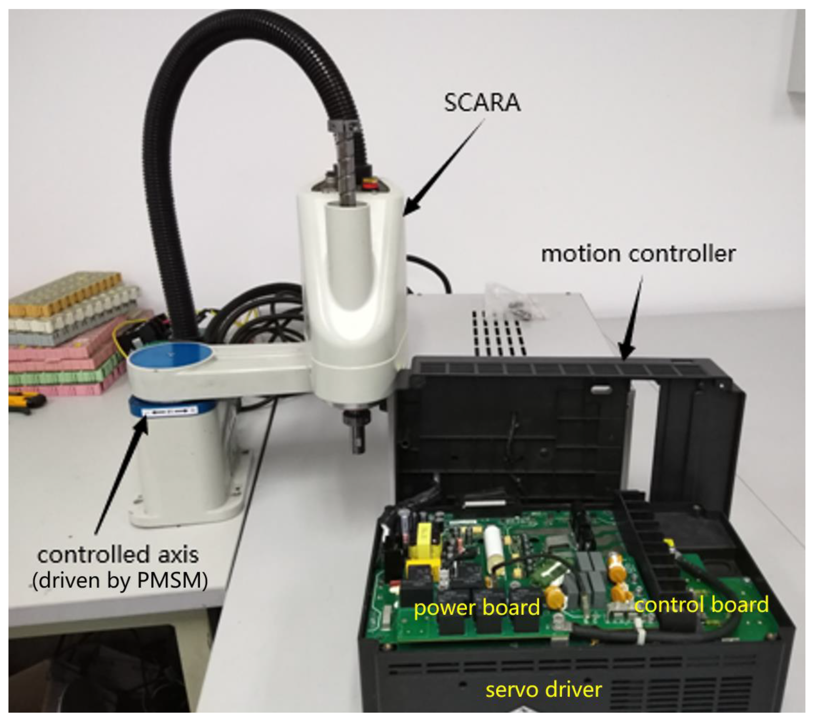
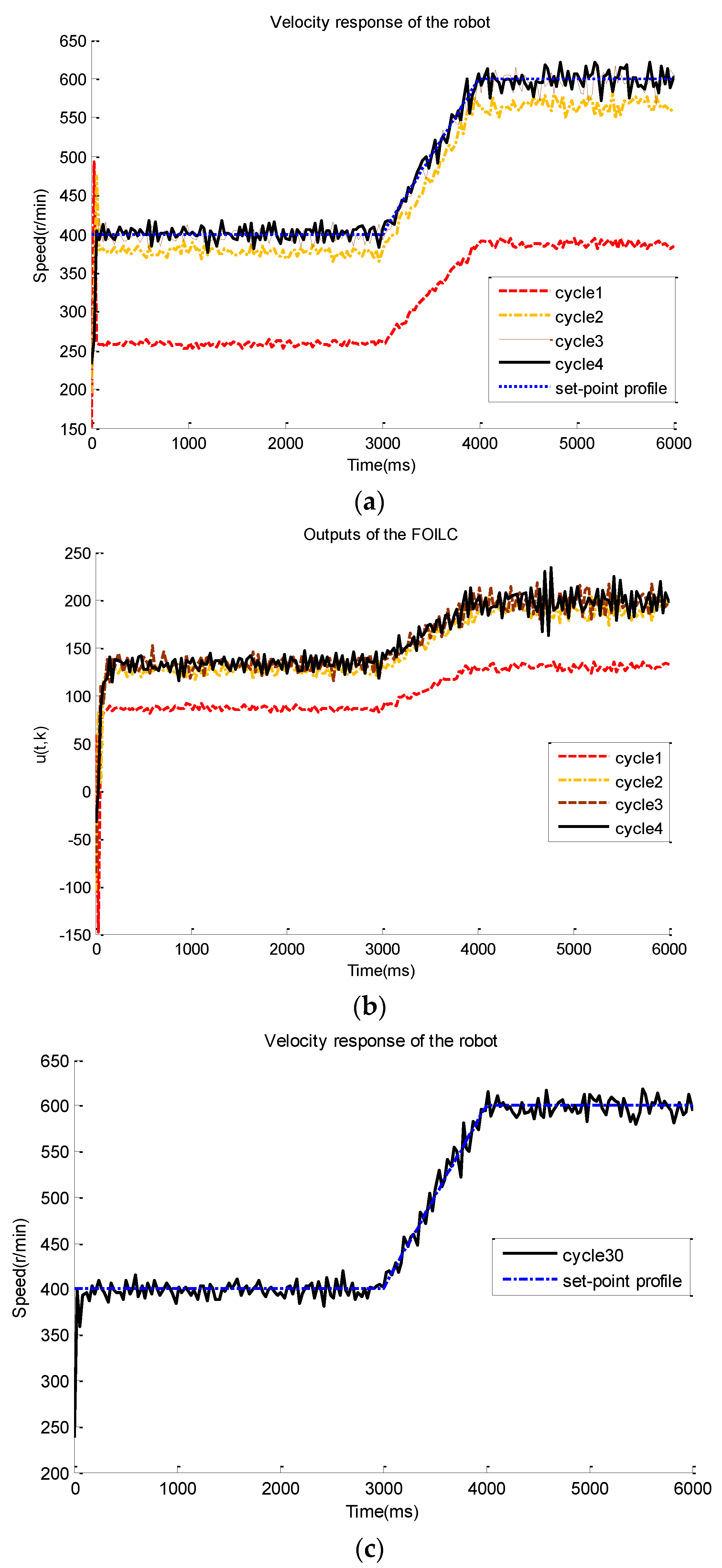
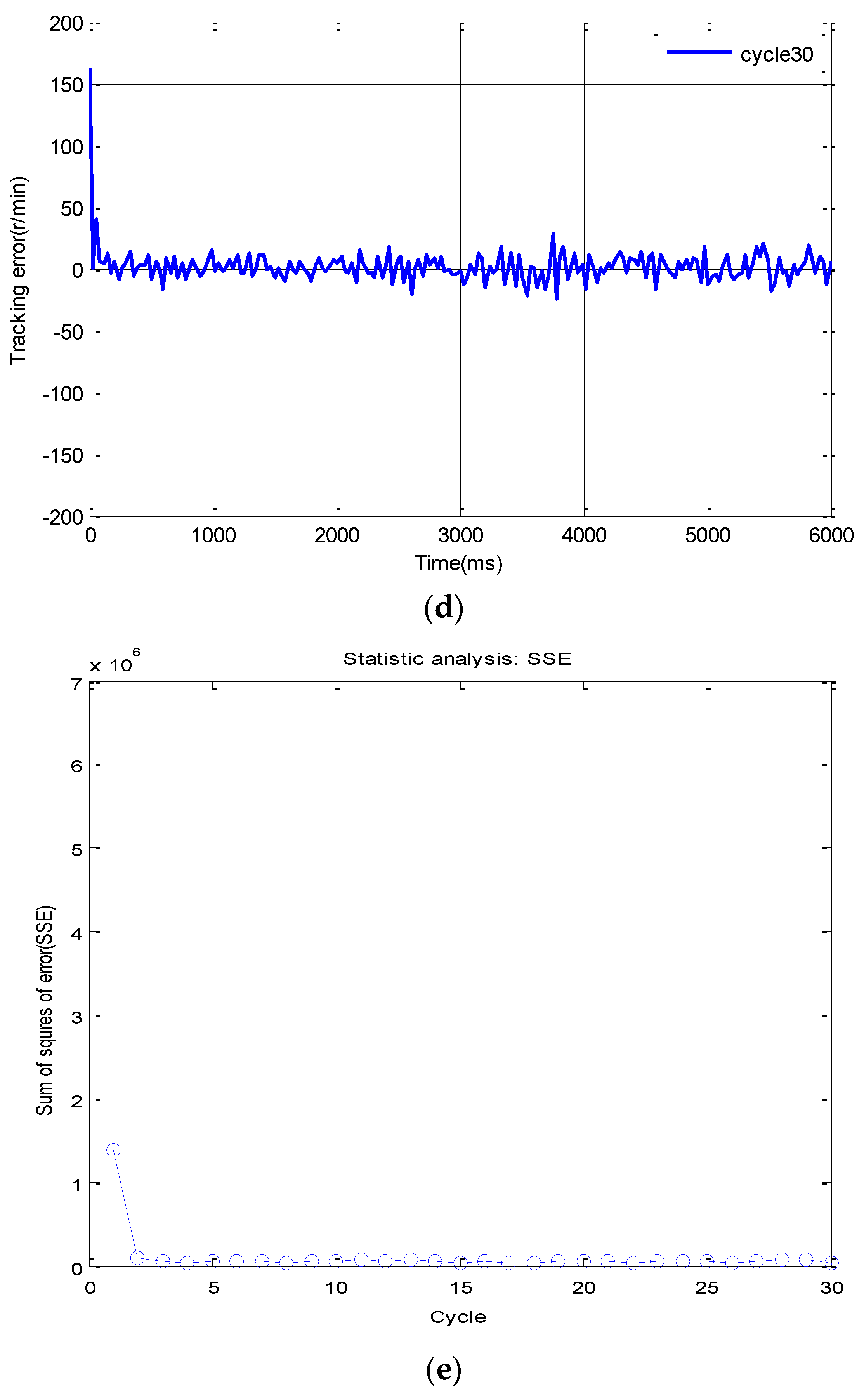
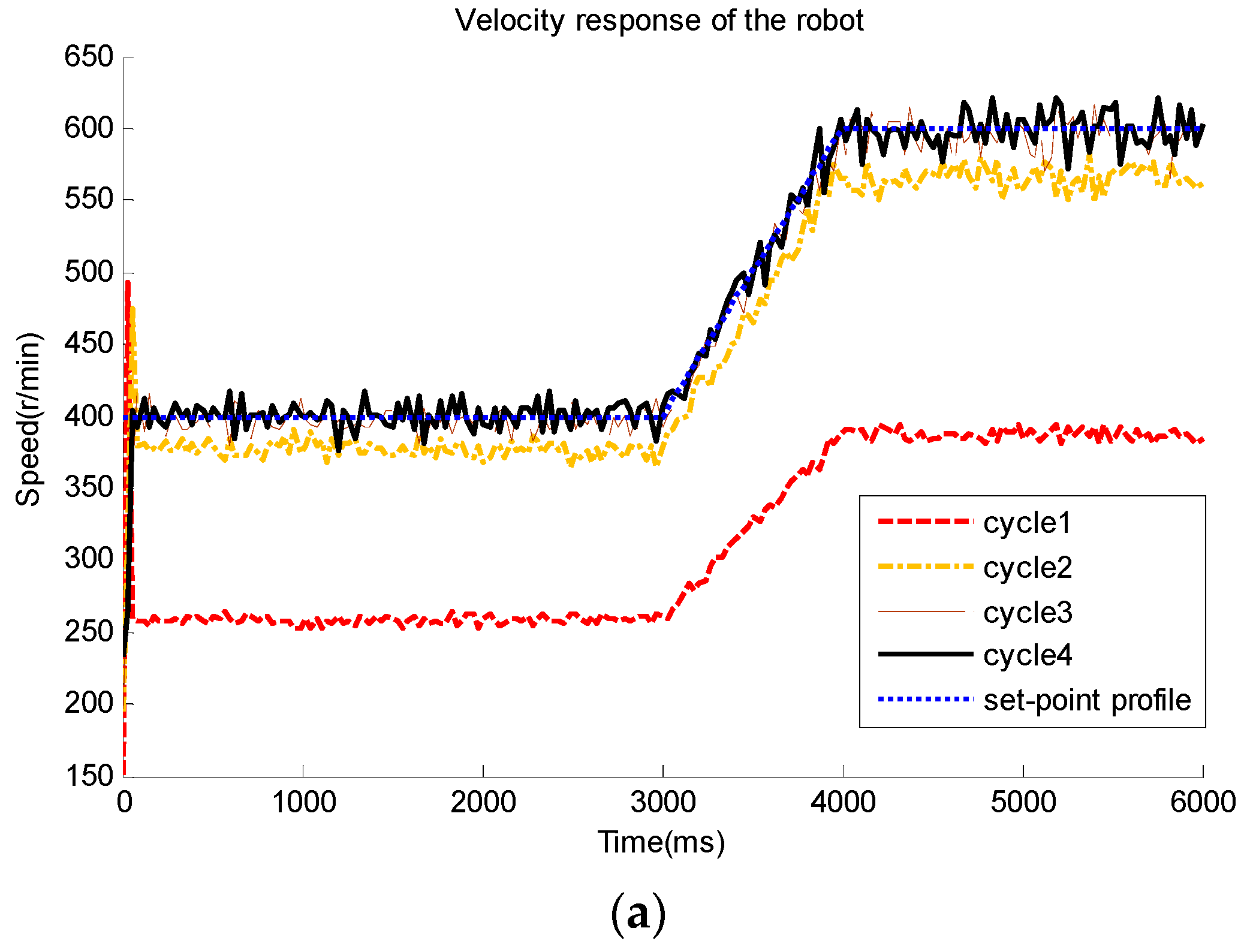
7. Experimental Results

The FOILC scheme proposed in this paper have been experimentally validated using the robot system and compared with IOILC algorithm proposed in reference [36]. The configuration of the four degrees-of-freedom SCARA robot is shown in Figure 4. Experiments are focused on controlling one of the axes depicted in Figure 4 denoted by “controlled axis”, which is driven by a permanent magnet synchronous motor (PMSM). The motion controller and servo driver are both based on “TMSC320F28335” DSP. The motion controller sets a reference value, and the servo driver receives the given value through field bus communication. The speed of controlled axis is obtained by differentiating angular displacement, which is detected by the resolver.

The state–space equation of the controlled axis is modeled based on step response tests, which is converted as (48). The performance parameters are given the same as simulations parameters, which result in the same control parameters with simulations. The set-point profiles are as follows:

$$Y_r=\left\{\begin{array}{cc}400,& 0<t\le 3000\\ 0.2\times (t-3000)+400,& 3000<t\le 4000\\ 600,& 4000<t\le 6000\end{array}\right.$$

(52)

Given $\tau =\theta =0.868$, ${\omega }_c=70$, ${\varnothing }_m=70$.

Using the proposed tuning algorithm can obtain the following control parameters under ideal conditions.

The control parameters of FOILC are obtained as (50) and (51).

The experimental result of step and slope responses by the FOILC for the speed control of the robot are depicted in Figure 5. It can be observed from Figure 5a that the outputs of the system converge quickly, and the control performance is optimized from cycle 1 to cycle 4. Figure 5c,d show that the velocity response can quickly follow the set-point profile when the trial number increases to 30. In Figure 5e, the sum-of-squares error (SSE) standards is used to measure the output tracking error along the batch direction. It can be seen from Figure 5 that perfect tracking has reached nearly the fifth cycles. In addition, there is no steady-state output tracking error from the first cycle.

The results of velocity responses by the IOILC designed following the reference [36] procedure are illustrated in Figure 6a, and the corresponding control inputs are plotted in Figure 6b. These experiments results show that the system output of the first cycle is far from the set point. The system output response converges rapidly after the fourth cycle, and the acceptable control performance is obtained in the 30th cycle, while the output tracking error in terms of SSE along the batch direction is plotted in Figure 6e. It can be seen from Figure 6 that there is no steady-state output tracking error from the fifth cycle.

Both of simulations and experiments results demonstrate the effectiveness of the proposed control schemes. Due to the ideal condition for the simulations, the design control approaches can obtain excellent control performance. Furthermore, experimental results with velocity response of robot show that the outputs can track the reference input quickly and stably despite existent nonlinear and time varying characteristics. These obtained results by comparing the proposed FOILC scheme with the previous IOILC indicate that the proposed FOILC has better control performance than that of the IOILC algorithm.

8. Conclusions

The FOILC scheme has been developed based on 2D system theory for the batch motion process in this paper. Moreover, the control parameters are tuned by LMIs and given specifications. The simulations and experimental results show that the proposed control scheme can achieve favorable performance for the speed control of robots. A comparison with an IOILC method clearly illustrates that the FOILC can track the set point in the 30th cycles to obtain very small tracking error, but the IOILC requires more than four cycles to reach favorable control performance. Importantly, FOILC exhibits better robust performance than IOILC. These obtained results further prove that FOILC adopts the proposed enhanced error function to replace the error of IOILC, which not only has faster response, but also has stronger robustness to reject the parameter variations and external disturbance. It should be further noted that the results obtained by the method proposed in this paper are limited to the variations of system parameters and external disturbances satisfying certain conditions. Therefore, our future work is to broaden the applicability of the proposed method to system parameter changes and external disturbances.

References

1. Sammons, P.M.; Gegel, M.L.; Bristow, D.A.; Landers, R.G. Repetitive Process Control of Additive Manufacturing with Application to Laser Metal Deposition. IEEE Trans. Control Syst. Technol. 2019, 27, 566–575. [Google Scholar] [CrossRef]
2. Mooren, N.; Witvoet, G.; Oomen, T. Gaussian process repetitive control: Beyond periodic internal models through kernels. Automatica 2022, 140, 1–13. [Google Scholar] [CrossRef]
3. Steinbuch, M. Repetitive control for systems with uncertain period-time. Automatica 2002, 38, 2103–2109. [Google Scholar] [CrossRef]
4. Moore, K.L.; Dahleh, M.; Bhattacharyya, S.P. Iterative learning control: A survey and new results. J. Robot. Syst. 1992, 9, 563–594. [Google Scholar] [CrossRef]
5. Yao, J.; Jiao, Z.; Ma, D. A Practical Nonlinear Adaptive Control of Hydraulic Servomechanisms with Periodic-Like Disturbances. IEEE/ASME Trans. Mechatron. 2015, 20, 2752–2760. [Google Scholar] [CrossRef]
6. Arimoto, S.; Kawamura, S.; Miyazaki, F. Bettering operation of robots by learning. J. Robot. Syst. 1984, 1, 123–140. [Google Scholar] [CrossRef]
7. Xu, J.-X.; Bien, Z.Z. The frontiers of iterative learning control. In Iterative Learning Control: Analysis, Design, Integration and Application; Kluwer Academic Publishers: Boston, MA, USA; Dordrecht, The Netherlands; London, UK, 1998; pp. 9–35. [Google Scholar]
8. Amann, N.; Owens, D.H.; Rogers, E. Iterative learning control using optimal feedback and feedforward actions. Int. J. Control 1996, 65, 277–293. [Google Scholar] [CrossRef]
9. Amann, N.; Owens, D.H.; Rogers, E. Predictive optimal iterative learning control. Int. J. Control 1998, 69, 203–226. [Google Scholar] [CrossRef]
10. Moon, J.-H.; Doh, T.-Y.; Chung, M.J. A robust approach to iterative learning control design for uncertain systems. Automatica 1998, 34, 1001–1004. [Google Scholar] [CrossRef]
11. Tayebi, A.; Zaremba, M.B. Robust iterative learning control design is straightforward for uncertain LTI systems satisfying the robust performance condition. IEEE Trans. Autom. Control 2003, 48, 101–106. [Google Scholar] [CrossRef]
12. Shi, J.; Gao, F.; Wu, T.-J. Robust design of integrated feedback and iterative learning control of a batch process based on a 2D Roesser system. J. Process Control 2005, 15, 907–924. [Google Scholar] [CrossRef]
13. Shi, J.; Zhou, H.; Cao, Z.; Jiang, Q. A design method for indirect iterative learning control based on two-dimensional generalized predictive control algorithm. J. Process Control 2014, 24, 1527–1537. [Google Scholar] [CrossRef]
14. Li, D.W.; Xi, Y.G.; Lu, J.Y.; Gao, F.R. Synthesis of real-time feedback-based 2Diterative learning control model predictive control for constrained batch processes with unknown input nonlinearity. Ind. Eng. Chem. Res. 2016, 55, 13074–13084. [Google Scholar] [CrossRef]
15. Han, C.; Jia, L.; Peng, D.G. Model predictive control of batch processes based on two-dimensional integration frame. Nonlinear Anal. Hybrid Syst. 2018, 28, 75–86. [Google Scholar] [CrossRef]
16. Zhang, R.; Wu, S.; Tao, J. A new design of predictive functional control strategy for batch processes in the two-dimensional framework. IEEE Trans. Ind. Inform. 2019, 15, 2905–2914. [Google Scholar] [CrossRef]
17. Hao, S.; Liua, T.; Gao, F. PI based indirect-type iterative learning control for batch processes with time-varying uncertainties: A 2D FM model based approach. J. Process Control 2019, 78, 57–67. [Google Scholar] [CrossRef]
18. Wang, Y.; Zhang, H.; Wei, S.; Zhou, D.; Huang, B. Control performance assessment for ILC-controlled batch processes in a 2-D system framework. IEEE Trans. Syst. Man Cybern. 2018, 48, 1493–1504. [Google Scholar] [CrossRef]
19. Zhou, L.; Jia, L.; Wang, Y.-L. An integrated robust iterative learning control strategy for batch processes based on 2D system. J. Process Control 2020, 85, 136–148. [Google Scholar] [CrossRef]
20. Hao, S. Two-dimensional delay compensation based iterative learning control scheme for batch processes with both input and state delays. J. Frankl. Inst. 2019, 356, 8118–8137. [Google Scholar] [CrossRef]
21. Shen, Y.; Wang, L.; Yu, J.; Zhang, R.; Gao, F. A hybrid 2D fault-tolerant controller design for multi-phase batch processes with time delay. J. Process Control. 2018, 69, 138–157. [Google Scholar] [CrossRef]
22. Wu, S.; Zhang, R. A two-dimensional design of model predictive control for batch processes with two-dimensional (2D) dynamics using extended non-minimal state space structure. J. Process Control 2019, 81, 172–189. [Google Scholar] [CrossRef]
23. Mandra, S.; Galkowski, K.; Rogers, E.; Rauh, A.; Aschemann, H. Performance-Enhanced Robust Iterative Learning Control with Experimental Application to PMSM Position Tracking. IEEE Trans. Control Syst. Technol. 2019, 27, 1813–1819. [Google Scholar] [CrossRef]
24. Li, Y.; Chen, Y.Q.; Ahn, H.-S. Fractional-order iterative learning control for fractional-order linear systems. Asian J. Control 2011, 13, 1–10. [Google Scholar] [CrossRef]
25. Sabatier, J.; Agrawal, O.P.; Tenreiro Machado, J.A. (Eds.) Advances in Fractional Calculus: Theoretical Developments and Applications in Physics and Engineering; Springer: Dordrecht, The Netherlands, 2007. [Google Scholar]
26. Li, Y.; Chen, Y.; Ahn, H.-S. A Survey on Fractional-Order Iterative Learning Control. J. Optim. Theory Appl. 2013, 156, 127–140. [Google Scholar] [CrossRef]
27. Chen, Y.Q.; Moore, K.L. On Dα-type iterative learning control. Proc. IEEE Conf. Decis. Control. 2001, 5, 4451–4456. [Google Scholar]
28. Ye, Y.; Tayebi, A.; Liu, X. All-pass filtering in iterative learning control. Automatica 2009, 45, 257–264. [Google Scholar] [CrossRef]
29. Ahmed, E.; El-Sayed, A.M.A.; El-Saka, H.A.A. Equilibrium points, stability and numerical solutions of fractional-order predator prey and rabies models. J. Math. Anal. 2007, 325, 542–553. [Google Scholar] [CrossRef]
30. Lan, Y.-H. Iterative learning control with initial state learning for fractional order nonlinear systems. Comput. Math. Appl. 2012, 64, 3210–3216. [Google Scholar] [CrossRef]
31. Yan, L.; Wei, J. Fractional order nonlinear systems with delay in iterative learning control. Appl. Math. Comput. 2015, 257, 546–552. [Google Scholar] [CrossRef]
32. Liu, S.; Wang, J.R. Fractional order iterative learning control with randomly varying trial lengths. J. Frankl. Inst. 2017, 354, 967–992. [Google Scholar] [CrossRef]
33. Luo, D.; Wang, J.; Shen, D. Iterative learning control for fractional-order multi-agent systems. J. Frankl. Inst. 2019, 356, 6328–6351. [Google Scholar] [CrossRef]
34. Luo, D.; Wang, J.; Shen, D. Iterative Learning Control for Locally Lipschitz Nonlinear Fractional-order Multi-agent Systems. J. Frankl. Inst. 2020, 357, 6671–6693. [Google Scholar] [CrossRef]
35. Mandra, S.; Galkowski, K.; Aschemann, H. Robust guaranteed cost ILC with dynamic feedforward and disturbance compensation for accurate PMSM position control. Control Eng. Pract. 2017, 65, 36–47. [Google Scholar] [CrossRef]
36. Du, C.; Xie, L.; Zhang, C. H∞ control and robust stabilization of two-dimensional systems in Roesser models. Automatica 2001, 37, 205–211. [Google Scholar] [CrossRef]
37. Cao, Y.Y.; Sun, Y.X.; Lam, J. Delay dependent robust H∞ for uncertain systems with time-varying delays. IEEE Proc. Control Theory Appl. 1998, 143, 338–344. [Google Scholar] [CrossRef]
38. Boyd, S.; Ghaoui, L.E.; Feron, E.; Balakrishnan, V. Linear Matrix Inequalities in System and Control Theory; SIAM: Philadelphia, PA, USA, 1994. [Google Scholar]
Figure 1. System framework of FOILC.
Fractalfract 07 00624 g001
Figure 2. Comparison of control performance between the proposed FOILC and previous IOILC [36]. (a) Step responses for the speed control of the robot model with FOILC (left) or IOILC (right); (b) Control output of the FOILC (left) or IOILC (right); (c) Tracking error for response with the FOILC (left) or IOILC (right).
Fractalfract 07 00624 g002
Figure 3. Signal of disturbance (d(t)).
Fractalfract 07 00624 g003
Figure 4. SCARA robot plant.
Fractalfract 07 00624 g004
Figure 5. Step and slope responses for the speed control of the robot with FOILC: (a) outputs of the robot from cycle 1 to cycle 4; (b) output of the FOILC from cycle 1 to cycle 4; (c) output of the robot in the cycle 30; (d) tracking error in the 30cycle; (e) Sum-of-squares error of the output following the input in the 30 cycles.
Fractalfract 07 00624 g005aFractalfract 07 00624 g005b
Figure 6. Step and slope responses for the speed control of the robot with IOILC [36]: (a) outputs of the robot from cycle 1 to cycle 4; (b) outputs of the IOILC from cycle 1 to cycle 4; (c) output of the robot in the cycle 30; (d) tracking error in the 30cycle; (e) Sum-of-squares error of the output following input in the 30 cycles.
Fractalfract 07 00624 g006aFractalfract 07 00624 g006bFractalfract 07 00624 g006c
Disclaimer/Publisher’s Note: The statements, opinions and data contained in all publications are solely those of the individual author(s) and contributor(s) and not of MDPI and/or the editor(s). MDPI and/or the editor(s) disclaim responsibility for any injury to people or property resulting from any ideas, methods, instructions or products referred to in the content.