Solving Generalized Heat and Generalized Laplace Equations Using Fractional Fourier Transform

Abstract

In the present work, the main objective is to find the solution of the generalized heat and generalized Laplace equations using the fractional Fourier transform, which is a general form of the solution of the heat equation and Laplace equation using the classical Fourier transform. We also formulate its solution using a sampling formula related to the fractional Fourier transform. The fractional Fourier transform is introduced, and related theorems and essential properties are collected. Several results related to the sampling formula are derived. A few examples are presented to illustrate the effectiveness and powerfulness of the proposed method compared to the classical Fourier transform method.

1. Introduction

As is well known, the fractional Fourier transform is a generalization of the classical Fourier transform. The fractional Fourier transform is a rapidly developing branch of mathematics, and has become a powerful method for various applications arising in many areas of science and engineering. This is because the transformation becomes very captivating. In recent years, some researchers have been trying to extend several applications of the Fourier transform to the fractional Fourier transform. In Refs. [1,2,3,4,5], the authors applied the fractional Fourier transform to optical signal processing. The authors of [6,7] discussed the use of the fractional Fourier transform in quantum mechanics. Until now, in the literature, very little work has been reported on the application of the fractional Fourier transform in partial differential equation problems. For example, the authors of [8] utilized the fractional Fourier transform to find the solution of the wave equation. The solution can be considered an extension of the solution of the wave equation using the classical Fourier transform. The authors of [9,10] generalized the solutions of the heat and wave equations using the linear canonical transform and the quadratic-phase Fourier transform, respectively. However, solutions of the heat and Laplace equations using the fractional Fourier transform do not exist as far as we know. Therefore, our current work focuses on the solution of the generalized heat and Laplace equations using the fractional Fourier transform method. To accomplish this, we first provide the definition of the fractional Fourier transform, as well as related theorems, and construct a basic relationship between the convolution theorem for the fractional Fourier transform and the convolution theorem for the classical Fourier transform. Then, we develop the results and relationship to obtain the solutions of the generalized heat and Laplace equations. Several examples are also demonstrated to verify the validity and applicability of the proposed approach compared to the classical Fourier transform.

The remaining parts of the present paper are organized as follows. In Section 2, we present some preliminaries that will be useful in this paper. The definition of the fractional Fourier transform and its useful properties are provided in Section 3. Section 4 is devoted to finding the solution of the generalized heat and Laplace equations using the fractional Fourier transform. Section 5 discusses the solution of the generalized heat equation using the sampling formula. Section 6 discusses a future research direction. Section 7 draws conclusions.

2. Notations

Let us first state a few notations and lemmas, which will be used throughout article.

Definition 1.

For $1\le s<\infty$, the Banach space $L^s\left(\mathbb{R}\right)$ of measurable functions is defined on $\mathbb{R}$ with the norm

$${\Vert f\Vert }_{L^s\left(\mathbb{R}\right)}={\left({\int }_{\mathbb{R}}{|f\left(x\right)|}^{s}dx\right)}^{\frac{1}{s}}<\infty .$$

(1)

In particular, $L^2\left(\mathbb{R}\right)$ is a Hilbert space with the usual inner product

$$\langle f,g\rangle ={\int }_{\mathbb{R}}f\left(x\right)\overline{g\left(x\right)}dx.$$

Now, we recall the definition of the Fourier transform (FT) and the related lemmas.

Definition 2.

The Fourier transform of a function $f\in L^1\left(\mathbb{R}\right)$ is defined by

$$\widehat{f}\left(\omega \right)=\mathcal{F}\left\{f\right\}\left(\omega \right)=\frac{1}{\sqrt{2\pi }}{\int }_{\mathbb{R}}{e}^{-i\omega x}f\left(x\right)dx,\omega \in \mathbb{R},$$

(2)

and for any $f,\widehat{f}\in L^1\left(\mathbb{R}\right)$, then its inversion formula is calculated by

$$f\left(x\right)={\mathcal{F}}^{-1}\left\{\widehat{f}\left(\omega \right)\right\}\left(x\right)=\frac{1}{\sqrt{2\pi }}{\int }_{\mathbb{R}}{e}^{i\omega x}\widehat{f}\left(\omega \right)d\omega ,x\in \mathbb{R}.$$

(3)

Lemma 1.

The Fourier transformation of a Gaussian function is given by

$$\mathcal{F}\left\{e^{-\alpha x^2}\right\}\left(\omega \right)=\frac{1}{\sqrt{2\alpha }}{e}^{-\frac{{\omega }^2}{4\alpha }},$$

(4)

where $\alpha >0$. 

Lemma 2.

The Fourier transformation of the Poisson kernel is given by

$$\mathcal{F}\left\{\sqrt{\frac{2}{\pi }}\frac{y}{x^2+y^2}\right\}\left(\omega \right)=e^{-y\left|\omega \right|}.$$

(5)

Definition 3.

Let $f\in L^1\left(\mathbb{R}\right)$. The translation, modulation, and dilation operators of the function f are expressed as follows

$$T_{a}f\left(x\right)=f\left(x-a\right),M_{b}f\left(x\right)=e^{ibx}f\left(x\right),D_{c}f\left(x\right)=\frac{1}{\sqrt{\left|c\right|}}f\left(\frac{x}{c}\right).$$

(6)

where $a,b,c$ are real constants. 

Definition 4.

Let $f,g\in L^1\left(\mathbb{R}\right)$, the convolution of the functions f and g denoted by $f\ast g$, be defined as

$$\left(f\ast g\right)\left(x\right)=\frac{1}{\sqrt{2\pi }}{\int }_{\mathbb{R}}f\left(t\right)g\left(x-t\right)dt,$$

(7)

and

$$(f\ast g)\left(x\right)={\mathcal{F}}^{-1}\left\{\mathcal{F}\left\{f\right\}\left(\omega \right)\mathcal{F}\left\{g\right\}\left(\omega \right)\right\}\left(x\right).$$

(8)

3. Fractional Fourier Transform and Properties

In what follows, we provide a definition of the fractional Fourier transform (FrFT), as well as the related theorems and properties. For more details, see the references [1,3,11,12,13,14,15,16,17,18,19,20,21,22,23,24,25,26].

Definition 5.

The one-dimensional fractional Fourier transform with angle θ of $f\in L^1\left(\mathbb{R}\right)$ denoted by ${\mathcal{F}}^{\theta }\left\{f\right\}\left(\omega \right)={\widehat{f}}^{\theta }\left(\omega \right)$ is defined as

$${\mathcal{F}}^{\theta }\left\{f\right\}\left(\omega \right)={\widehat{f}}^{\theta }\left(\omega \right)={\int }_{\mathbb{R}}{K}^{\theta }(x,\omega )f\left(x\right)dx,$$

(9)

where the kernel $K^{\theta }(x,\omega )$ is given by

$$K^{\theta }(x,\omega )=\left\{\begin{array}{cc}{C}^{\theta }{e}^{i(x^2+{\omega }^2)\frac{cot\theta }{2}-ix\omega csc\theta },& \theta \ne n\pi \hfill \\ \delta (x-\omega ),& \theta =2n\pi \hfill \\ \delta (x+\omega ),& \theta =(2n+1)\pi ,n\in Z\hfill \end{array},\right.$$

(10)

for which

$$C^{\theta }={(2\pi isin\theta )}^{-1/2}{e}^{i\theta /2}=\sqrt{\frac{1-icot\theta }{2\pi }}.$$

The inversion formula of the FrFT is described by

$$f\left(x\right)={\mathcal{F}}^{-1}\left\{{\widehat{f}}^{\theta }\left(\omega \right)\right\}\left(x\right)={\int }_{\mathbb{R}}\overline{K^{\theta }(x,\omega )}{\widehat{f}}^{\theta }\left(\omega \right)d\omega ,$$

(11)

where

$$\overline{K^{\theta }(x,\omega )}=\overline{C^{\theta }}{e}^{-i(x^2+{\omega }^2)\frac{cot\theta }{2}+ix\omega csc\theta }=K^{-\theta }(x,\omega ),$$

The relation between the FT and the FrFT is

$$\mathcal{F}\left\{r\right\}(\omega csc\theta )={(2\pi isin\theta )}^{\frac{1}{2}}{e}^{-\frac{i\theta }{2}}{e}^{-i{\omega }^2\frac{cot\theta }{2}}{\mathcal{F}}^{\theta }\left\{f\right\}\left(\omega \right),$$

(12)

where

$$r\left(x\right)=f\left(x\right)e^{i{x}^2\frac{cot\theta }{2}}.$$

(13)

Some useful properties of the FrFT are summarized in the following results.

Theorem 1

(Translation property). If $\varphi \in L^1\left(\mathbb{R}\right)$, then for any nonzero constant $r\in \mathbb{R}$, one has

$${\mathcal{F}}^{\theta }\left\{\varphi \left(x-r\right)\right\}\left(\omega \right)=e^{\frac{i}{4}\left(r^{2}sin2\theta -4\omega rsin\theta \right)}{\mathcal{F}}^{\theta }\left\{\varphi \left(x\right)\right\}\left(\omega -rcos\theta \right).$$

(14)

Theorem 2

(Modulation property). If $\varphi \in L^1\left(\mathbb{R}\right)$ and $m\in \mathbb{Z}$, then

$${\mathcal{F}}^{\theta }\left\{\varphi \left(x\right)e^{imx}\right\}\left(\omega \right)=e^{\frac{i}{4}\left(4\omega mcos\theta -m^{2}sin2\theta \right)}{\mathcal{F}}^{\theta }\left\{\varphi \left(x\right)\right\}(\omega -msin\theta ).$$

(15)

Theorem 3

(Dilation Property). If $\varphi \in L^1\left(\mathbb{R}\right)$, then for any nonzero constant $k\in \mathbb{R}$, we have

$${\mathcal{F}}^{\theta }\left\{\varphi \left(kx\right)\right\}\left(\omega \right)=\frac{C^{\theta }}{k{C}^{{\theta }_0}}{e}^{\frac{i{k}^2{\omega }^2}{2}\left(1-\left(\frac{{sec}^2\theta }{{sec}^2{\theta }_0}\right)\right)cot{\theta }_0}{\mathcal{F}}^{{\theta }_0}\left\{\varphi \left(x\right)\right\}\left(\frac{ksec\theta }{{sec\theta }_0}\omega \right),$$

(16)

where

$${\theta }_0={cot}^{-1}\left(\frac{cot\theta }{k^2}\right).$$

Theorem 4

(Moment property). If $\varphi \in L^1\left(\mathbb{R}\right)$, then we have

$${\mathcal{F}}^{\theta }\left\{x\varphi \right\}\left(\omega \right)=\omega sec\theta \left({\mathcal{F}}^{\theta }\left\{\varphi \right\}\right)\left(\omega \right)+\frac{i}{cot\theta }{\mathcal{F}}^{\theta }\left\{\frac{d\varphi \left(x\right)}{dx}\right\}\left(\omega \right).$$

(17)

Definition 6

(Convolution definition). Suppose that $\varphi ,\phi \in L^1\left(\mathbb{R}\right)$. The convolution operator related to the FrFT is defined as

$$\left(\varphi ★\phi \right)\left(x\right)={\int }_{\mathbb{R}}\varphi \left(t\right)\phi (x-t)\sqrt{\frac{1-icot\theta }{2\pi }}{e}^{it(t-x)cot\theta }dt.$$

(18)

As an immediate consequence of Definition 6, we obtain the next theorem.

Theorem 5

(Convolution theorem). With the above notation, one obtains

$${\mathcal{F}}^{\theta }\left\{(\varphi ★\phi )\right\}\left(\omega \right)=e^{\frac{-i{\omega }^{2}cot\theta }{2}}{\mathcal{F}}^{\theta }\left\{\varphi \right\}\left(\omega \right){\mathcal{F}}^{\theta }\left\{\phi \right\}\left(\omega \right).$$

(19)

Definition 7.

The Schwartz space $\mathcal{S}$($\mathbb{R}$) of rapidly decaying functions is defined by a collection of complex-valued functions satisfying

$$\mathcal{S}=\left\{\varphi \left(x\right)\in C^{\infty }\left(\mathbb{R}\right):\underset{x\in \mathbb{R}}{sup}|x^m{D}^m\varphi \left(x\right)|<\infty ,\forall m,n\in \mathbb{N}\right\},$$

(20)

where $D=\frac{d}{dx}$. 

Definition 8.

The Schwartz space ${\mathcal{S}}_{\theta }$($\mathbb{R}$) of rapidly decaying functions related to the FrFT is defined by a collection of complex-valued functions satisfying

$${\mathcal{S}}_{\theta }=\left\{\varphi \left(x\right)\in C^{\infty }\left(\mathbb{R}\right):\underset{x\in \mathbb{R}}{sup}|x^m{\overline{D}}_x^n\varphi \left(x\right)|<\infty ,\forall m,n\in \mathbb{N}\right\},$$

where ${\overline{D}}_x=\frac{d}{dx}-ixcot\theta$. 

Theorem 6.

Let $K^{\theta }(x,\omega )$ be the kernel of the fractional Fourier transform and ${\overline{D}}_x^r=$${(\frac{d}{dx}-ixcot\theta )}^r$, then for $\forall r\in {\mathbb{N}}_0$ we have 

1. 

${\overline{D}}_x^r{K}^{\theta }(x,\omega )={(-i\omega csc\theta )}^r{K}^{\theta }(x,\omega )$

2. 

${\int }_{\mathbb{R}}{\overline{D}}_x^r{K}^{\theta }(x,\omega )f\left(x\right)dx={\int }_{\mathbb{R}}{K}^{\theta }(x,\omega ){\left({\overline{D}}_x^{\ast }\right)}^{r}f\left(x\right)dx$

3. 

${\mathcal{F}}^{\theta }\left\{{\left({\overline{D}}_x^{\ast }\right)}^{r}f\left(x\right)\right\}\left(\omega \right)={(-i\omega csc\theta )}^r{\mathcal{F}}^{\theta }\left\{f\left(x\right)\right\}\left(\omega \right)$, 

where

$${\overline{D}}_x^{\ast }=-\left(\frac{d}{dx}+ixcot\theta \right).$$

(21)

Proof. 

1.

Direct computation shows

$$\begin{array}{cc}\hfill \frac{d}{dx}(K^{\theta }(x,\omega )& =\frac{d}{dx}\left(C^{\theta }{e}^{i(x^2+{\omega }^2)\frac{cot\theta }{2}-ix\omega csc\theta }\right)\hfill \\ \hfill & =C^{\theta }\frac{d}{dx}\left(e^{i(x^2+{\omega }^2)\frac{cot\theta }{2}-ix\omega csc\theta }\right)\hfill \\ \hfill & =C^{\theta }\left(e^{i(x^2+{\omega }^2)\frac{cot\theta }{2}-ix\omega csc\theta }\right)i\left(xcot\theta -\omega csc\theta \right)\hfill \\ \hfill & =K^{\theta }(x,\omega )(ixcot\theta -i\omega csc\theta ).\hfill \end{array}$$

This means that

$$\left(\frac{d}{dx}-ixcot\theta \right)K^{\theta }(x,\omega )=(-i\omega csc\theta )K^{\theta }(x,\omega ).$$

Continuing in this way, we obtain

$${\left(\frac{d}{dx}-ixcot\theta \right)}^r{K}^{\theta }(x,\omega )={(-i\omega csc\theta )}^r{K}^{\theta }(\theta ,\omega ).$$

2.

Observe first that

$$\begin{array}{cc}\hfill {\int }_{\mathbb{R}}{\overline{D}}_x{K}^{\theta }(x,\omega )f\left(x\right)dx& ={\int }_{\mathbb{R}}\left(\frac{d}{dx}-ixcot\theta \right)K^{\theta }(x,\omega )f\left(x\right)dx\hfill \\ \hfill & ={\int }_{\mathbb{R}}\left(\frac{d}{dx}{K}^{\theta }(x,\omega )f\left(x\right)\right)dx-{\int }_{\mathbb{R}}ixcot\theta K^{\theta }(x,\omega )f\left(x\right)dx\hfill \\ \hfill & =-{\int }_{\mathbb{R}}{K}^{\theta }(x,\omega )\left(\frac{d}{dx}f\left(x\right)\right)dx-{\int }_{\mathbb{R}}ixcot\theta K^{\theta }(x,\omega )f\left(x\right)dx\hfill \\ \hfill & =-{\int }_{\mathbb{R}}{K}^{\theta }(x,\omega )\left(\frac{d}{dx}+ixcot\theta \right)f\left(x\right)dx\hfill \\ \hfill & ={\int }_{\mathbb{R}}{K}^{\theta }(x,\omega ){\overline{D}}^{\ast }f\left(x\right)dx.\hfill \end{array}$$

Then, we obtain

$${\int }_{\mathbb{R}}{\overline{D}}_x^r{K}^{\theta }(x,\omega )f\left(x\right)dx={\int }_{\mathbb{R}}{K}^{\theta }(x,\omega ){\left({\overline{D}}^{\ast }\right)}^{r}f\left(x\right)dx.$$

(22)

3.

Using the previous results, we arrive at

$$\begin{array}{cc}\hfill {\mathcal{F}}^{\theta }\left\{{\left({\overline{D}}_x^{\ast }\right)}^{r}f\left(x\right)\right\}\left(\omega \right)& ={\int }_{\mathbb{R}}{K}^{\theta }(x,\omega ){\left({\overline{D}}_x^{\ast }\right)}^{r}f\left(x\right)dx\hfill \\ \hfill & ={\int }_{\mathbb{R}}{\overline{D}}_x^r{K}^{\theta }(x,\omega )f\left(x\right)dx\hfill \\ \hfill & ={(-i\omega csc\theta )}^r{\int }_{\mathbb{R}}{K}^{\theta }(x,\omega )f\left(x\right)dx\hfill \\ \hfill & ={(-i\omega csc\theta )}^r{\mathcal{F}}^{\theta }\left\{f\left(x\right)\right\}\left(\omega \right).\hfill \end{array}$$

□

4. Fractional Fourier Transform for Generalized Heat and Laplace Equations

In this section, we utilize the fractional Fourier transform (FrFT) to solve the generalized heat and Laplace equations. First, we formulate the one-dimensional heat equation in the FrFT domain. We then present some examples to illustrate the powerfulness of the proposed FrFT.

4.1. Fractional Fourier Transform Method for Heat Equation

Let us now consider a one-dimensional heat equation in the fractional Fourier transform (FrFT) domain as follows

$$\frac{\partial u(x,t)}{\partial t}=c^2{\left({\overline{D}}_x^{\ast }\right)}^{2}u(x,t),-\infty <x<\infty ,t>0.$$

(23)

In this case, the initial condition $u(x,0)=f\left(x\right)\in L^1\left(\mathbb{R}\right)$, and ${\overline{D}}_x^{\ast }$ is defined by (21) with c being any constant.

Remark 1.

It is not difficult to see that relation (23) can be written in the form

$$\begin{array}{cc}\hfill u(x,t)& =c^2{u}_{xx}(x,t)\hfill \\ \hfill & =2cot\theta c^2\left(2i{u}_x(x,t)-cot\theta u(x,t)\right).\hfill \end{array}$$

This partial differential equation is the unsteady heat conduction equation. In this case, $u(x,t)$ is the temperature at position x and time t and $c^{2}cot\theta$ is the thermal conductivity of the media depending on θ. 

Further, for $\theta =\frac{\pi }{2}$, the unsteady heat equation becomes

$$u_t(x,t)-c^2{u}_{xx}(x,t)=0$$

which is the steady heat equation.

Taking the FrFT on both sides of Equation (23) with respect to x, we obtain

$${\int }_{\mathbb{R}}{K}^{\theta }(x,\omega )\frac{\partial u(x,t)}{\partial t}dx=c^2{\int }_{\mathbb{R}}{K}^{\theta }(x,\omega ){\left({\overline{D}}_x^{\ast }\right)}^{2}u(x,t)dx.$$

This equation can be expressed as

$$\begin{array}{cc}\hfill \frac{\partial {\widehat{u}}^{\theta }(\omega ,t)}{\partial t}& =c^2{\int }_{\mathbb{R}}{\left({\overline{D}}_x^{\ast }\right)}^2{K}^{\theta }(t,\omega )u(x,t)dx\hfill \\ \hfill & =-c^2{\omega }^2{csc}^2\theta {\widehat{u}}^{\theta }(\omega ,t).\hfill \end{array}$$

(24)

Therefore,

$${\widehat{u}}^{\theta }(\omega ,t)=C{e}^{(-c^2{\omega }^2{csc}^2\theta )t},$$

(25)

where C is an arbitrary constant.

Next, using the initial condition $u(x,0)=f\left(x\right)$, we find that

$${\widehat{u}}^{\theta }(\omega ,0)={\int }_{\mathbb{R}}{K}^{\theta }(x,\omega )f\left(x\right)dx=C.$$

(26)

Substituting (26) into (25) results in

$${\widehat{u}}^{\theta }(\omega ,t)=\left({\int }_{\mathbb{R}}{K}^{\theta }(x,\omega )f\left(x\right)dx\right)e^{(-c^2{\omega }^2{csc}^2\theta )t}.$$

(27)

Taking the inverse of the FrFT in (27), we see that

$$u(x,t)={\mathcal{F}}^{-\theta }\left\{{\widehat{u}}^{\theta }(\omega ,t)\right\}(x,t).$$

(28)

Due to Equation (11), we further obtain

$$\begin{array}{cc}\hfill u(x,t)& ={\mathcal{F}}^{-\theta }\left\{\left({\int }_{\mathbb{R}}{K}^{\theta }(x,\omega )f\left(x\right)dx\right)e^{(-c^2{\omega }^2{csc}^2\theta )t}\right\}(x,t)\hfill \\ \hfill & =\overline{C^{\theta }}{\int }_{\mathbb{R}}{e}^{-i(x^2+{\omega }^2)\frac{cot\theta }{2}+ix\omega csc\theta }\left({\int }_{\mathbb{R}}{K}^{\theta }(x,\omega )f\left(x\right)dx\right)e^{(-c^2{\omega }^2{csc}^2\theta )t}d\omega \hfill \\ \hfill & =\overline{C^{\theta }}{C}^{\theta }{\int }_{\mathbb{R}}{e}^{-i(x^2+{\omega }^2)\frac{cot\theta }{2}+ix\omega csc\theta }\left({\int }_{\mathbb{R}}{e}^{i(x^2+{\omega }^2)\frac{cot\theta }{2}-ix\omega csc\theta }f\left(x\right)dx\right)e^{(-c^2{\omega }^2{csc}^2\theta )t}d\omega \hfill \\ \hfill & =\frac{1}{2\pi sin\theta }{\int }_{\mathbb{R}}{e}^{-i(x^2+{\omega }^2)\frac{cot\theta }{2}+ix\omega csc\theta }\left({\int }_{\mathbb{R}}{e}^{i(x^2+{\omega }^2)\frac{cot\theta }{2}-ix\omega csc\theta }f\left(x\right)dx\right)e^{(-c^2{\omega }^2{csc}^2\theta )t}d\omega \hfill \\ \hfill & =\frac{e^{\frac{-i{x}^{2}cot\theta }{2}}}{2\pi sin\theta }{\int }_{\mathbb{R}}{e}^{ix\omega csc\theta }\left({\int }_{\mathbb{R}}{e}^{\frac{i{x}^{2}cot\theta }{2}}{e}^{-ix\omega csc\theta }f\left(x\right)dx\right)e^{(-c^2{\omega }^2{csc}^2\theta )t}d\omega .\hfill \end{array}$$

(29)

Denote

$$h^{\theta }\left(x\right)=e^{\frac{i{x}^{2}cot\theta }{2}}f\left(x\right),$$

(30)

and

$$\omega csc\theta =v.$$

(31)

Now Equation (29) above will lead to

$$\begin{array}{cc}\hfill u(x,t)& =\frac{e^{\frac{-i{x}^{2}cot\theta }{2}}}{2\pi sin\theta }sin\theta {\int }_{\mathbb{R}}{e}^{ixv}{e}^{-c^2{v}^{2}t}dv{\int }_{\mathbb{R}}{e}^{-ixv}{h}^{\theta }\left(x\right)dx\hfill \\ \hfill & =\frac{e^{\frac{-i{x}^{2}cot\theta }{2}}}{2\pi }{\int }_{\mathbb{R}}{e}^{ixv}{e}^{-c^2{v}^{2}t}dv{\int }_{\mathbb{R}}{e}^{-ixv}{h}^{\theta }\left(x\right)dx\hfill \\ \hfill & =\frac{e^{\frac{-i{x}^{2}cot\theta }{2}}}{\sqrt{2\pi }}{\int }_{\mathbb{R}}{e}^{ixv}{e}^{-c^2{v}^{2}t}\left(\frac{1}{\sqrt{2\pi }}{\int }_{\mathbb{R}}{e}^{-ixv}{h}^{\theta }\left(x\right)dx\right)dv\hfill \\ \hfill & =\frac{e^{\frac{-i{x}^{2}cot\theta }{2}}}{\sqrt{2\pi }}{\int }_{\mathbb{R}}{e}^{ixv}{e}^{-c^2{v}^{2}t}\mathcal{F}\left\{h^{\theta }\left(x\right)\right\}dv.\hfill \end{array}$$

(32)

By virtue of Equation (4), we obtain

$$\mathcal{F}\left\{\frac{1}{\sqrt{2c^{2}t}}{e}^{-\frac{x^2}{4c^{2}t}}\right\}=e^{-c^2{v}^{2}t}.$$

(33)

Substituting Equation (33) into Equation (32) results in

$$\begin{array}{cc}\hfill u(x,t)& =\frac{e^{\frac{-i{x}^{2}cot\theta }{2}}}{\sqrt{2\pi }}{\int }_{\mathbb{R}}\mathcal{F}\left\{\frac{1}{\sqrt{2c^{2}t}}{e}^{-\frac{x^2}{4c^{2}t}}\right\}\mathcal{F}\left\{h^{\theta }\left(x\right)\right\}{e}^{ixv}dv\hfill \\ \hfill & =\frac{e^{\frac{-i{x}^{2}cot\theta }{2}}}{\sqrt{2\pi }\sqrt{2c^{2}t}}{\int }_{\mathbb{R}}\mathcal{F}\left\{e^{-\frac{x^2}{4c^{2}t}}\right\}\mathcal{F}\left\{h^{\theta }\left(x\right)\right\}{e}^{ixv}dv\hfill \end{array}$$

(34)

An application of Equation (8) on Equation (34) results in

$$\begin{array}{cc}\hfill u(x,t)& =\frac{e^{\frac{-i{x}^{2}cot\theta }{2}}}{\sqrt{2c^{2}t}}{\mathcal{F}}^{-1}\left\{\mathcal{F}\left\{e^{-\frac{x^2}{4c^{2}t}}\right\}\mathcal{F}\left\{h^{\theta }\left(x\right)\right\}\right\}(x,t)\hfill \\ \hfill & =\frac{e^{\frac{-i{x}^{2}cot\theta }{2}}}{\sqrt{2c^{2}t}}\left(e^{-\frac{x^2}{4c^{2}t}}\ast h^{\theta }\left(x\right)\right)\left(y\right)\hfill \\ \hfill & =\frac{e^{\frac{-i{x}^{2}cot\theta }{2}}}{\sqrt{2c^{2}t}}\left(e^{\frac{-x^2}{4c^{2}t}}\ast e^{\frac{i{x}^{2}cot\theta }{2}}f\left(x\right)\right)\left(y\right)\hfill \\ \hfill & =\frac{e^{\frac{-i{x}^{2}cot\theta }{2}}}{\sqrt{4\pi c^{2}t}}{\int }_{\mathbb{R}}{e}^{-\frac{{(x-y)}^2}{4c^{2}t}}{e}^{\frac{i{y}^{2}cot\theta }{2}}f\left(y\right)dy.\hfill \end{array}$$

(35)

In the special case, when $\theta =\frac{\pi }{2}$, relation (34) above is reduced to

$$u(x,t)=\frac{1}{\sqrt{4\pi c^{2}t}}{\int }_{\mathbb{R}}{e}^{-\frac{{(x-y)}^2}{4c^{2}t}}f\left(y\right)dy,$$

(36)

which is the solution of the heat equation using the classical Fourier transform.

To illustrate the above result, we present the following example.

Example 1.

Find the solution $u(x,t)$ of (35) with $c=1$ and

$$f\left(x\right)=\left\{\begin{array}{cc}1,& \left|x\right|<1\hfill \\ 0,& otherwise.\hfill \end{array}\right.$$

(37)

Solution. Substituting (37) into (35), we find

$$\begin{array}{cc}\hfill u(x,t)& =\frac{e^{\frac{-i{x}^{2}cot\theta }{2}}}{\sqrt{4\pi t}}{\int }_{-1}^1{e}^{\frac{-{\left(x-y\right)}^2}{4t}}{e}^{\frac{i{y}^{2}cot\theta }{2}}dy\hfill \\ \hfill & =\frac{e^{\frac{-i{x}^{2}cot\theta }{2}}}{\sqrt{4\pi t}}{\int }_{-1}^1{e}^{\frac{-y^2}{4t}+i{y}^2\frac{cot\theta }{2}+\frac{2xy}{4t}}{e}^{\frac{-x^2}{4t}}dy\hfill \\ \hfill & =\frac{e^{\frac{-i{x}^{2}cot\theta }{2}-\frac{x^2}{4t}}}{\sqrt{4\pi t}}{\int }_{-1}^1{e}^{-y^2(\frac{1}{4t}-i\frac{cot\theta }{2})+\frac{2xy}{4t}}dy.\hfill \end{array}$$

(38)

Equation (41) can be rewritten in the form

$$\begin{array}{cc}\hfill u(x,t)& =\frac{e^{\frac{-i{x}^{2}cot\theta }{2}-\frac{x^2}{4t}}}{\sqrt{4\pi t}}{\int }_{-1}^1{e}^{-(\frac{1}{4t}-i\frac{cot\theta }{2})\left(y^2-\frac{2xy}{4t\left(\frac{1}{4t}-\frac{icot\theta }{2}\right)}\right)}dy\hfill \\ \hfill & =\frac{e^{\frac{-i{x}^{2}cot\theta }{2}-\frac{x^2}{4t}}}{\sqrt{4\pi t}}{\int }_{-1}^1{e}^{-(\frac{1}{4t}-i\frac{cot\theta }{2})\left(y^2-\frac{2xy}{1-i2tcot\theta }\right)}dy.\hfill \end{array}$$

(39)

The above equation will lead to

$$\begin{array}{cc}\hfill u(x,t)& =\frac{e^{\frac{-i{x}^{2}cot\theta }{2}-\frac{x^2}{4t}}}{\sqrt{4\pi t}}{\int }_{-1}^1{e}^{-(\frac{1}{4t}-i\frac{cot\theta }{2})\left({\left(\frac{x}{1-i2tcot\theta }-y\right)}^2-{\left(\frac{x}{1-i2tcot\theta }\right)}^2\right)}dy\hfill \\ \hfill & =\frac{e^{\frac{-i{x}^{2}cot\theta }{2}-\frac{x^2}{4t}}}{\sqrt{4\pi t}}{\int }_{-1}^1{e}^{-(\frac{1}{4t}-i\frac{cot\theta }{2}){\left(\frac{x}{1-i2tcot\theta }-y\right)}^2}{e}^{(\frac{1}{4t}-i\frac{cot\theta }{2}){\left(\frac{x}{1-i2tcot\theta }\right)}^2}dy\hfill \\ \hfill & =\frac{e^{\frac{-i{x}^{2}cot\theta }{2}-\frac{x^2}{4t}+\left(\frac{1}{4t}-\frac{icot\theta }{2}\right){\left(\frac{x}{1-i2tcot\theta }\right)}^2}}{\sqrt{4\pi t}}{\int }_{-1}^1{e}^{-(\frac{1}{4t}-i\frac{cot\theta }{2}){\left(\frac{x}{1-i2tcot\theta }-y\right)}^2}dy\hfill \\ \hfill & =\frac{e^{\frac{-i{x}^{2}cot\theta }{2}-\frac{x^2}{4t}+\left(\frac{1}{4t}-\frac{icot\theta }{2}\right){\left(\frac{x}{1-i2tcot\theta }\right)}^2}}{\sqrt{4\pi t}}{\int }_{-1}^1{e}^{-{\left(\frac{\sqrt{\frac{1}{4t}-\frac{icot\theta }{2}}x}{1-i2tcot\theta }-\sqrt{\frac{1}{4t}-\frac{icot\theta }{2}}y\right)}^2}dy.\hfill \end{array}$$

(40)

If we denote

$$z=\frac{\sqrt{\frac{1}{4t}-\frac{icot\theta }{2}}x}{1-i2tcot\theta }-\sqrt{\frac{1}{4t}-\frac{icot\theta }{2}}y,$$

then

$$\begin{array}{cc}\hfill u(x,& t)\hfill \\ \hfill =& \frac{e^{\frac{-i{x}^{2}cot\theta }{2}-\frac{x^2}{4t}+\left(\frac{1}{4t}-\frac{icot\theta }{2}\right){\left(\frac{x}{1-i2tcot\theta }\right)}^2}}{\sqrt{4\pi t}}{\int }_{\frac{\sqrt{\frac{1}{4t}-\frac{icot\theta }{2}}x}{1-i2tcot\theta }-\sqrt{\frac{1}{4t}-\frac{icot\theta }{2}}}^{\frac{\sqrt{\frac{1}{4t}-\frac{icot\theta }{2}}x}{1-i2tcot\theta }+\sqrt{\frac{1}{4t}-\frac{icot\theta }{2}}}{e}^{-z^2}\frac{dz}{\sqrt{\frac{1}{4t}-\frac{icot\theta }{2}}}\hfill \\ \hfill =& \frac{e^{\frac{-i{x}^{2}cot\theta }{2}-\frac{x^2}{4t}+\left(\frac{1}{4t}-\frac{icot\theta }{2}\right){\left(\frac{x}{1-i2tcot\theta }\right)}^2}}{\sqrt{4\pi t}\sqrt{\frac{1}{4t}-\frac{icot\theta }{2}}}\hfill \\ \hfill & \times \left(\frac{\sqrt{\pi }}{2}\left(erf\left[\frac{\sqrt{\frac{1}{4t}-\frac{icot\theta }{2}}x}{1-i2tcot\theta }+\sqrt{\frac{1}{4t}-\frac{icot\theta }{2}}\right]-erf\left[\frac{\sqrt{\frac{1}{4t}-\frac{icot\theta }{2}}x}{1-i2tcot\theta }-\sqrt{\frac{1}{4t}-\frac{icot\theta }{2}}\right]\right)\right).\hfill \end{array}$$

(41)

Hence,

$$\begin{array}{cc}\hfill u(x,& t)\hfill \\ \hfill & =\frac{e^{\frac{-i{x}^{2}cot\theta }{2}-\frac{x^2}{4t}+\left(\frac{1}{4t}-\frac{icot\theta }{2}\right){\left(\frac{x}{1-i2tcot\theta }\right)}^2}}{2\sqrt{4t}\sqrt{\frac{1}{4t}-\frac{icot\theta }{2}}}\hfill \\ \hfill & \times \left(erf\left[\frac{\sqrt{\frac{1}{4t}-\frac{icot\theta }{2}}x}{1-i2tcot\theta }+\sqrt{\frac{1}{4t}-\frac{icot\theta }{2}}\right]-erf\left[\frac{\sqrt{\frac{1}{4t}-\frac{icot\theta }{2}}x}{1-i2tcot\theta }-\sqrt{\frac{1}{4t}-\frac{icot\theta }{2}}\right]\right).\hfill \end{array}$$

(42)

Here,

$$erf\left(\omega \right)=\frac{2}{\sqrt{\pi }}{\int }_0^{\omega }{e}^{-z^2}dz,$$

(43)

for all $\omega$. Simulation of (42) at various values of $\theta$ and $c=1$ is shown in

Table 1. The solutions obtained for Example 1 with various values of $\theta$ and $c=1$.

$\mathit{\theta }$	c	$\mathit{u}(\mathit{x},\mathit{t})$
$\frac{\pi }{2}$	1	$\frac{1}{2}\left(erf\left(\frac{x+1}{2\sqrt{t}}\right)-erf\left(\frac{x-1}{2\sqrt{t}}\right)\right)$
$\frac{\pi }{3}$	1	$\frac{e^{-\frac{t{x}^2}{\sqrt{3}(\sqrt{3}-i2t)}}}{2\sqrt{\frac{\sqrt{3}-i2t}{\sqrt{3}}}}\left(erf\left(\frac{\sqrt{3}x}{\sqrt{12t-i8\sqrt{3}{t}^2}}+\sqrt{\frac{\sqrt{3}-i2t}{4\sqrt{3}t}}\right)-erf\left(\frac{\sqrt{3}x}{\sqrt{12t-i8\sqrt{3}{t}^2}}-\sqrt{\frac{\sqrt{3}-i2t}{4\sqrt{3}t}}\right)\right)$
$\frac{\pi }{4}$	1	$\frac{e^{-\frac{t{x}^2}{1-i2t}}}{2\sqrt{1-i2t}}\left(erf\left(\frac{x+(1-i2t)}{\sqrt{4t-i8t^2}}\right)-erf\left(\frac{x-(1-i2t)}{\sqrt{4t-i8t^2}}\right)\right)$
$\frac{\pi }{6}$	1	$\frac{e^{-\frac{3t{x}^2}{1-i2\sqrt{3}t}}}{2\sqrt{1-i2\sqrt{3}t}}\left(erf\left(\frac{x}{\sqrt{4t-i8\sqrt{3}{t}^2}}+\sqrt{\frac{1-i2\sqrt{3}t}{4t}}\right)-erf\left(\frac{x}{\sqrt{4t-i8\sqrt{3}{t}^2}}-\sqrt{\frac{1-i2\sqrt{3}t}{4t}}\right)\right)$

.

In Table 1, it seems that for $\theta =\frac{\pi }{2}$ Equation (41) boils down to

$$u(x,t)=\frac{1}{2}\left[erf\left(\frac{x+1}{2\sqrt{t}}\right)-erf\left(\frac{x-1}{2\sqrt{t}}\right)\right],$$

(44)

which is quite similar to the solution of the classical heat equation using the Fourier transform as shown in Figure 1. Figure 2 and Figure 3 display the solution of Example 1 for various values of $\theta$ and t.

Now, let us consider the heat equation with a nonconstant coefficient as follows

$$\frac{\partial u(x,t)}{\partial t}=t{\left({\overline{D}}_x^{\ast }\right)}^{2}u(x,t),-\infty <x<\infty ,t>0$$

(45)

with the initial condition $u(x,0)=f\left(x\right)$, and ${\overline{D}}_x^{\ast }=-\left(\frac{\mathrm{d}}{\mathrm{d}x}+ixcot\left(\theta \right)\right)$.

Using the same procedure, we obtain

$$u(x,t)=\frac{e^{\frac{-i{x}^{2}cot\theta }{2}}}{t\sqrt{2\pi }}{\int }_{\mathbb{R}}{e}^{-\frac{{(x-y)}^2}{2t^2}}{e}^{\frac{i{y}^{2}cot\theta }{2}}f\left(y\right)dy.$$

(46)

4.2. Fractional Fourier Transform Method for Generalized Laplace Equation

Consider the following one-dimensional Laplace equation in the FrFT domain

$${\left({\overline{D}}_x^{\ast }\right)}^{2}u(x,y)+u_{yy}=0,-\infty <x<\infty ,y>0,$$

(47)

with initial condition

$$u(x,0)=f\left(x\right)\in L^1\left(\mathbb{R}\right),-\infty <x<\infty$$

$$\underset{y\to \infty }{\lim }u(x,y)=0,\underset{\left|x\right|\to \infty }{\lim }u(x,y)=0.$$

Let us explore the solution of the generalized Laplace equation mentioned above. Observe first that

$${\mathcal{F}}^{\theta }\left\{{\left({\overline{D}}_x^{\ast }\right)}^{2}u(x,y)\right\}(\omega ,y)=-{\omega }^2{csc}^2\theta {\widehat{u}}^{\theta }(\omega ,y)$$

(48)

and

$${\mathcal{F}}^{\theta }\left\{u_{yy}\right\}=\frac{{\partial }^2{\widehat{u}}^{\theta }(\omega ,y)}{\partial y^2}.$$

(49)

Taking the FrFT on both sides of (47) with respect to x, and then including Equations (48) and (49) into Equation (47), it is easily seen that

$$\frac{{\partial }^2{\widehat{u}}^{\theta }(\omega ,y)}{\partial y^2}={\omega }^2{csc}^2\theta {\widehat{u}}^{\theta }(\omega ,y).$$

(50)

The general solution of (50) is

$${\widehat{u}}^{\theta }(\omega ,y)=A\left(\omega \right)e^{csc\left(\theta \right)\omega y}+B\left(\omega \right)e^{-csc\left(\theta \right)\omega y},$$

(51)

for some undetermined coefficient functions $A\left(\omega \right)$ and $B\left(\omega \right)$. To obtain these coefficients, we use the boundary condition

$$\underset{y\to \infty }{\lim }u(x,y)=0$$

and

$$\underset{y\to \infty }{\lim }{\widehat{u}}^{\theta }(\omega ,y)=0.$$

This implies that $A\left(\omega \right)=0$ for $\omega >0$ and $B\left(\omega \right)=0$ for $\omega <0$. Hence,

$${\widehat{u}}^{\theta }(\omega ,y)=C\left(\omega \right)e^{-csc\left(\theta \right)\left|\omega \right|y}$$

(52)

for $C\left(\omega \right)=A\left(\omega \right),\omega <0$ dan $C\left(\omega \right)=B\left(\omega \right),\omega >0$.

Next, based on the initial condition $u(x,0)=f\left(x\right)$, we obtain

$${\widehat{u}}^{\theta }(\omega ,0)={\int }_{\mathbb{R}}{K}^{\theta }(x,\omega )f\left(x\right)dx=C\left(\omega \right).$$

(53)

Taking the inverse transform of the FrFT defined by (11), we arrive at

$$\begin{array}{cc}\hfill u(x,y)& ={\mathcal{F}}^{-\theta }\left\{\widehat{f}\left(\omega \right)e^{-csc\left(\theta \right)\left|\omega \right|y}\right\}\hfill \\ \hfill & ={\mathcal{F}}^{-\theta }\left\{\left({\int }_{\mathbb{R}}{K}^{\theta }(x,\omega )f\left(x\right)dx\right)e^{-csc\left(\theta \right)\left|\omega \right|y}\right\}\hfill \\ \hfill & =\overline{C^{\theta }}{\int }_{\mathbb{R}}{e}^{-i(x^2+{\omega }^2)\frac{cot\theta }{2}+ix\omega csc\theta }\left({\int }_{\mathbb{R}}{K}^{\theta }(x,\omega )f\left(x\right)dx\right)e^{-csc\left(\theta \right)\left|\omega \right|y}d\omega \hfill \\ \hfill & =\overline{C^{\theta }}{C}^{\theta }{\int }_{\mathbb{R}}{e}^{-i(x^2+{\omega }^2)\frac{cot\theta }{2}+ix\omega csc\theta }\left({\int }_{\mathbb{R}}{e}^{i(x^2+{\omega }^2)\frac{cot\theta }{2}-ix\omega csc\theta }f\left(x\right)dx\right)e^{-csc\left(\theta \right)\left|\omega \right|y}d\omega \hfill \\ \hfill & =\frac{1}{2\pi sin\theta }{\int }_{\mathbb{R}}{e}^{-i(x^2+{\omega }^2)\frac{cot\theta }{2}+ix\omega csc\theta }\left({\int }_{\mathbb{R}}{e}^{i(x^2+{\omega }^2)\frac{cot\theta }{2}-ix\omega csc\theta }f\left(x\right)dx\right)e^{-csc\left(\theta \right)\left|\omega \right|y}d\omega \hfill \\ \hfill & =\frac{e^{\frac{-i{x}^{2}cot\theta }{2}}}{2\pi sin\theta }{\int }_{\mathbb{R}}{e}^{ix\omega csc\theta }\left({\int }_{\mathbb{R}}{e}^{\frac{i{x}^{2}cot\theta }{2}}{e}^{-ix\omega csc\theta }f\left(x\right)dx)\right)e^{-csc\left(\theta \right)\left|\omega \right|y}d\omega .\hfill \end{array}$$

Due to Equations (30) and (31), we obtain

$$\begin{array}{cc}\hfill u(x,y)& =\frac{e^{\frac{-i{x}^{2}cot\theta }{2}}}{2\pi sin\theta }sin\theta {\int }_{\mathbb{R}}{e}^{ixv}{e}^{-\left|v\right|y}dv{\int }_{\mathbb{R}}{e}^{-ixv}{h}^{\theta }\left(x\right)dx\hfill \\ \hfill & =\frac{e^{\frac{-i{x}^{2}cot\theta }{2}}}{2\pi }{\int }_{\mathbb{R}}{e}^{ixv}{e}^{-\left|v\right|y}dv{\int }_{\mathbb{R}}{e}^{-ixv}{h}^{\theta }\left(x\right)dx\hfill \\ \hfill & =\frac{e^{\frac{-i{x}^{2}cot\theta }{2}}}{\sqrt{2\pi }}{\int }_{\mathbb{R}}{e}^{ixv}{e}^{-\left|v\right|y}\left(\frac{1}{\sqrt{2\pi }}{\int }_{\mathbb{R}}{e}^{-ixv}{h}^{\theta }\left(x\right)dx\right)dv\hfill \\ \hfill & =\frac{e^{\frac{-i{x}^{2}cot\theta }{2}}}{\sqrt{2\pi }}{\int }_{\mathbb{R}}{e}^{ixv}{e}^{-\left|v\right|y}\mathcal{F}\left\{h^{\theta }\left(x\right)\right\}dv.\hfill \end{array}$$

(54)

Applying (5) into (54), we obtain

$$\begin{array}{cc}\hfill u(x,y)& =\frac{e^{\frac{-i{x}^{2}cot\theta }{2}}}{\sqrt{2\pi }}{\int }_{\mathbb{R}}\mathcal{F}\left\{\sqrt{\frac{2}{\pi }}\frac{y}{x^2+y^2}\right\}\mathcal{F}\left\{h^{\theta }\left(x\right)\right\}{e}^{ixv}dv.\hfill \end{array}$$

(55)

An application of relations (3) and (8) to (55) leads to

$$\begin{array}{cc}\hfill u(x,y)& =e^{\frac{-i{x}^{2}cot\theta }{2}}{\mathcal{F}}^{-1}\left\{\mathcal{F}\left\{\sqrt{\frac{2}{\pi }}\frac{y}{x^2+y^2}\right\}\mathcal{F}\left\{h^{\theta }\left(x\right)\right\}\right\}\hfill \\ \hfill & =e^{\frac{-i{x}^{2}cot\theta }{2}}\left(\left(\sqrt{\frac{2}{\pi }}\frac{y}{x^2+y^2}\right)\ast h^{\theta }\left(x\right)\right)\left(s\right)\hfill \\ \hfill & =\frac{y{e}^{\frac{-i{x}^{2}cot\theta }{2}}}{\pi }{\int }_{\mathbb{R}}\frac{h^{\theta }\left(s\right)}{{(x-s)}^2+y^2}ds\hfill \\ \hfill & =\frac{y{e}^{\frac{-i{x}^{2}cot\theta }{2}}}{\pi }{\int }_{\mathbb{R}}\frac{e^{\frac{i{s}^{2}cot\theta }{2}}}{{(x-s)}^2+y^2}f\left(s\right)ds.\hfill \end{array}$$

(56)

In the special case, for $\theta =\frac{\pi }{2}$, relation (56) becomes

$$u(x,y)=\frac{y}{\pi }{\int }_{\mathbb{R}}\frac{1}{{(x-s)}^2+y^2}f\left(s\right)ds.$$

(57)

which is the solution of the classical Laplace equation using the Fourier transform (see [27]).

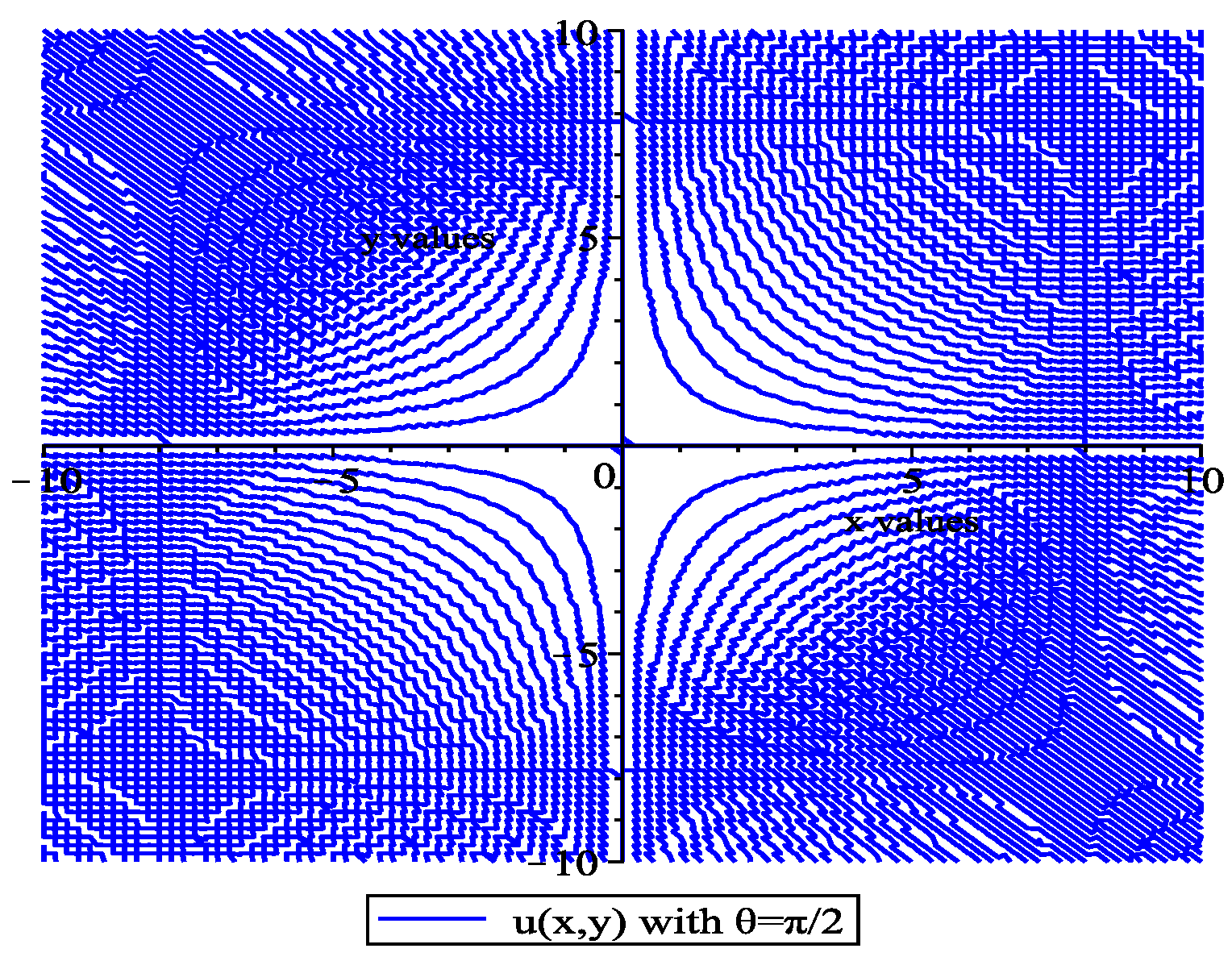
Example 2.

We will now solve the Dirichlet problem in the upper half plane of (56) above with the Gaussian function

$$f\left(x\right)=e^{-x^2}.$$

(58)

Solution. It is easy to verify that

$$\begin{array}{cc}\hfill {\int }_{\mathbb{R}}\frac{e^{i{s}^2\frac{cot\theta }{2}}}{{(x-s)}^2+y^2}{e}^{-s^2}ds=& {\int }_{\mathbb{R}}^{}\frac{e^{(i\frac{cot\theta }{2}-1)s^2}}{{(x-s)}^2+y^2}ds\hfill \\ \hfill =& \frac{\pi }{y}{e}^{-(x^2-y^2)-\frac{i{y}^{2}cot\theta }{2}}\left(e^{-i2xy-xycot\theta }-e^{i2xy+xycot\theta }\right).\hfill \end{array}$$

Substituting the above equation into (56), we obtain

$$\begin{array}{cc}\hfill u(x,y)=& e^{-(x^2-y^2)-\frac{i{y}^{2}cot\theta }{2}}\left(e^{-i2xy-xycot\theta }-e^{i2xy+xycot\theta }\right).\hfill \end{array}$$

(59)

Simulation of (59) at various values of $\theta$ is shown in

Table 2. The solutions obtained for Example 2 with various values of $\theta$.

$\mathit{\theta }$	$\mathit{u}(\mathit{x},\mathit{t})$
$\frac{\pi }{2}$	$-2isinxy{e}^{-(x^2-y^2)}$
$\frac{\pi }{3}$	$-e^{-(x^2-y^2)-\frac{i{y}^2}{2\sqrt{3}}}\left(e^{-i2xy-\frac{xy}{\sqrt{3}}}-e^{i2xy+\frac{xy}{\sqrt{3}}}\right)$
$\frac{\pi }{4}$	$-e^{-(x^2-y^2)-\frac{i{y}^2}{2}}\left(e^{-i2xy-xy}-e^{i2xy+xy}\right)$
$\frac{\pi }{6}$	$-e^{-(x^2-y^2)-\frac{i\sqrt{3}{y}^2}{2}}\left(e^{-i2xy-\sqrt{3}xy}-e^{i2xy+\sqrt{3}xy}\right)$

.

In Table 2, it seems that for $\theta =\frac{\pi }{2}$ Equation (59) above changes to

$$\begin{array}{c}\hfill u(x,y)=-2isinxy{e}^{-(x^2-y^2)}.\end{array}$$

(60)

Figure 4 and Figure 5 display the solution of Example 2 for $\theta =\frac{\pi }{4}$ and $\theta =\frac{\pi }{2}$, respectively. From Table 2, we may infer that relation (59) is more flexible than relation (60) due to the extra parameter $\theta$.

Let us now consider the following problem of (56) on a strip as follows

$${\left({\overline{D}}_x^{\ast }\right)}^{2}u(x,y)+u_{yy}=0,-\infty <x<\infty ,a<y<b,$$

(61)

with the initial condition

$$u(x,a)=f\left(x\right),u(x,b)=g\left(x\right),$$

(62)

where $f,g\in L^1\left(\mathbb{R}\right)$.

Taking the FrFT on both sides of (61) and (62) with respect to x, we obtain

$${\widehat{u}}^{\theta }(\omega ,y)=A\left(\omega \right)e^{y\omega csc\theta }+B\left(\omega \right)e^{-y\omega csc\theta },$$

(63)

where

$$\begin{array}{c}\hfill A\left(\omega \right)=\frac{{\widehat{f}}^{\theta }\left(\omega \right)e^{-\omega bcsc\left(\theta \right)}-{\widehat{g}}^{\theta }\left(\omega \right)e^{-\omega acsc\left(\theta \right)}}{2sinh\left(\omega \right(a-b)csc(\theta \left)\right)},\end{array}$$

(64)

and

$$\begin{array}{c}\hfill B\left(\omega \right)=-\frac{{\widehat{f}}^{\theta }\left(\omega \right)e^{\omega bcsc\left(\theta \right)}-{\widehat{g}}^{\theta }\left(\omega \right)e^{\omega acsc\left(\theta \right)}}{2sinh\left(\omega \right(a-b)csc(\theta \left)\right)}.\end{array}$$

(65)

Denote

$$\omega csc\theta =v,h_1^{\theta }\left(x\right)=e^{\frac{i{x}^{2}cot\theta }{2}}f\left(x\right),h_2^{\theta }\left(x\right)=e^{\frac{i{x}^{2}cot\theta }{2}}g\left(x\right),$$

(66)

we obtain

$$\begin{array}{c}\hfill {\widehat{f}}^{\theta }=C^{\theta }{e}^{\frac{i{\omega }^{2}cot\theta }{2}}{\int }_{\mathbb{R}}{e}^{-ixv}{h}_1^{\theta }\left(x\right)dx=C^{\theta }\sqrt{2\pi }{e}^{\frac{i{\omega }^{2}cot\theta }{2}}\mathcal{F}\left\{h_1^{\theta }\left(x\right)\right\}\left(v\right),\end{array}$$

(67)

and

$$\begin{array}{c}\hfill {\widehat{g}}^{\theta }=C^{\theta }{e}^{\frac{i{\omega }^{2}cot\theta }{2}}{\int }_{\mathbb{R}}{e}^{-ixv}{h}_2^{\theta }\left(x\right)dx=C^{\theta }\sqrt{2\pi }{e}^{\frac{i{\omega }^{2}cot\theta }{2}}\mathcal{F}\left\{h_2^{\theta }\left(x\right)\right\}\left(v\right).\end{array}$$

(68)

Substituting (67) and (68) into (64) and (65), respectively, we find that

$$A\left(\omega \right)=C^{\theta }\frac{\sqrt{2\pi }{e}^{\frac{i{\omega }^{2}cot\theta }{2}}\left(\mathcal{F}\left\{h_1^{\theta }\left(x\right)\right\}\left(v\right)e^{-bv}-\mathcal{F}\left\{h_2^{\theta }\left(x\right)\right\}\left(v\right)e^{-av}\right)}{2sinh\left(v\right(a-b\left)\right)},$$

(69)

$$B\left(\omega \right)=-C^{\theta }\frac{\sqrt{2\pi }{e}^{\frac{i{\omega }^{2}cot\theta }{2}}\left(\mathcal{F}\left\{h_1^{\theta }\left(x\right)\right\}\left(v\right)e^{bv}-\mathcal{F}\left\{h_2^{\theta }\left(x\right)\right\}\left(v\right)e^{av}\right)}{2sinh\left(v\right(a-b\left)\right)}.$$

(70)

With the help of the inverse transform of the FrFT defined by (11), we arrive at

$$\begin{array}{cc}\hfill u(x,y)=& {\mathcal{F}}^{-\theta }\left\{A\left(\omega \right)e^{vy}+B\left(\omega \right)e^{-vy}\right\}\hfill \\ \hfill =& \frac{e^{\frac{-i{x}^{2}cot\theta }{2}}}{\sqrt{2\pi }}{\int }_{\mathbb{R}}\frac{e^{ixv}\left(\mathcal{F}\left\{h_1^{\theta }\left(x\right)\right\}\left(v\right)e^{v(y-b)}-\mathcal{F}\left\{h_2^{\theta }\left(x\right)\right\}\left(v\right)e^{v(y-a)}\right)}{2sinh\left(v\right(a-b\left)\right)}dv\hfill \\ \hfill & -\frac{e^{\frac{-i{x}^{2}cot\theta }{2}}}{\sqrt{2\pi }}{\int }_{\mathbb{R}}\frac{e^{ixv}\left(\mathcal{F}\left\{h_1^{\theta }\left(x\right)\right\}\left(v\right)e^{v(b-y)}+\mathcal{F}\left\{h_2^{\theta }\left(x\right)\right\}\left(v\right)e^{v(a-y)}\right)}{2sinh\left(v\right(a-b\left)\right)}dv\hfill \\ \hfill =& \frac{e^{\frac{-i{x}^{2}cot\theta }{2}}}{\sqrt{2\pi }}\hfill \\ \hfill & \times {\int }_{\mathbb{R}}{e}^{ixv}\frac{\mathcal{F}\left\{h_1^{\theta }\left(x\right)\right\}\left(v\right)\left(e^{v(y-b)}-e^{-v(y-b)}\right)-\mathcal{F}\left\{h_2^{\theta }\left(x\right)\right\}\left(v\right)\left(e^{v(y-a)}-e^{-v(y-a)}\right)}{2sinh\left(v\right(a-b\left)\right)}dv\hfill \\ \hfill =& \frac{e^{\frac{-i{x}^{2}cot\theta }{2}}}{\sqrt{2\pi }}{\int }_{\mathbb{R}}{e}^{ixv}\frac{\mathcal{F}\left\{h_1^{\theta }\left(x\right)\right\}\left(v\right)sinh\left(v(y-b)\right)-\mathcal{F}\left\{h_2^{\theta }\left(x\right)\right\}\left(v\right)sinh\left(v(y-a)\right)}{sinh\left(v\right(a-b\left)\right)}dv.\hfill \end{array}$$

(71)

Now observe that

$$\begin{array}{cc}\hfill {\int }_{\mathbb{R}}\frac{sinh\left(v\right(y-b\left)\right)}{sinh\left(v\right(a-b\left)\right)}{e}^{ivx}dv& ={\int }_{\mathbb{R}}\frac{e^{v(y-b)}-e^{v(b-y)}}{e^{v(a-b)}-e^{v(b-a)}}{e}^{ivx}dv\hfill \\ \hfill & ={\int }_{\mathbb{R}}\frac{e^{v(y-b+ix)}-e^{v(b-y+ix)}}{e^{v(a-b)}-e^{v(b-a)}}dv.\hfill \end{array}$$

Putting $p=y-b+ix$, $q=b-y+ix$, $r=a-b$, and $s=b-a$, we obtain

$$\begin{array}{cc}\hfill {\int }_{\mathbb{R}}\frac{e^{pv}-e^{qv}}{e^{rv}-e^{sv}}dv& ={\int }_{\mathbb{R}}\frac{e^{(p-r)v}-e^{(q-r)v}}{1-e^{-(r-s)v}}dv\hfill \\ \hfill & ={\int }_{\mathbb{R}}\frac{e^{-(r-p)v}-e^{-(r-q)v}}{1-e^{(s-r)v}}dv.\hfill \end{array}$$

(72)

Letting $t=(r-s)v$, we see that

$$\begin{array}{cc}\hfill {\int }_{\mathbb{R}}\frac{e^{-\left(\frac{r-p}{r-s}\right)t}-e^{-\left(\frac{r-q}{r-s}\right)t}}{1-e^{-t}}\frac{dx}{r-s}& =\frac{1}{r-s}{\int }_{\mathbb{R}}\frac{e^{-\left(\frac{r-p}{r-s}\right)t}-e^{-\left(\frac{r-q}{r-s}\right)t}}{1-e^{-t}}dt\hfill \\ \hfill & =\frac{1}{r-s}\left(\psi \left(\frac{r-q}{r-s}\right)-\psi \left(\frac{r-p}{r-s}\right)\right),\hfill \end{array}$$

(73)

where

$$\psi \left(n\right)-\psi \left(m\right)={\int }_{\mathbb{R}}\frac{e^{-tm}-e^{-tn}}{1-e^{-t}}dt,m=\frac{a-2b+y-ix}{2(a-b)},n=\frac{a-y-ix}{2(a-b))}.$$

(74)

This means that

$$\mathcal{F}\left\{\frac{1}{\sqrt{2\pi }}\frac{1}{2(a-b)}\left(\psi \left(\frac{a-y-ix}{2(a-b))}\right)-\psi \left(\frac{a-2b+y-ix}{2(a-b)}\right)\right)\right\}=\frac{1}{\sqrt{2\pi }}\frac{sinh\left(v\right(y-b\left)\right)}{sinh\left(v\right(a-b\left)\right)}.$$

(75)

Using a similar procedure, we arrive at

$$\mathcal{F}\left\{\frac{1}{\sqrt{2\pi }}\frac{1}{2(a-b)}\left(\psi \left(\frac{2a-b-y-ix}{2(a-b)}\right)-\psi \left(\frac{b+y-ix}{2(a-b)}\right)\right)\right\}=\frac{1}{\sqrt{2\pi }}\frac{sinh\left(v\right(y-a\left)\right)}{sinh\left(v\right(a-b\left)\right)}.$$

(76)

Hence,

$$\begin{array}{cc}\hfill u(x,& y)\hfill \\ \hfill =& \frac{e^{\frac{-i{x}^{2}cot\theta }{2}}}{4\pi (a-b)}{\int }_{\mathbb{R}}^{}\left(\psi \left(\frac{a-y-i(x-s)}{2(a-b))}\right)-\psi \left(\frac{a-2b+y-i(x-s)}{2(a-b)}\right)\right)e^{\frac{i{s}^{2}cot\theta }{2}}f\left(s\right)ds\hfill \\ \hfill & -\frac{e^{\frac{-i{x}^{2}cot\theta }{2}}}{4\pi (a-b)}{\int }_{\mathbb{R}}^{}\left(\psi \left(\frac{2a-b-y-i(x-s)}{2(a-b))}\right)-\psi \left(\frac{b+y-i(x-s)}{2(a-b)}\right)\right)e^{\frac{i{s}^{2}cot\theta }{2}}g\left(s\right)ds.\hfill \end{array}$$

(77)

5. Relation to Sampling Theorem for FrFT

In this part, we first introduce the limited band for the fractional Fourier transform. We derive the following results, which will be useful for solving the discrete version of the generalized heat equation.

Definition 9.

A signal $f\left(t\right)$ is called band-limited related to the FrFT if there is a positive number σ satisfying ${\mathcal{F}}^{\theta }\left\{f\right\}\left(\omega \right)=0$ for all $|\omega |>\sigma$. 

Lemma 3.

(See [28,29]) Suppose $f\left(t\right)$ is band-limited to σ in the fractional Fourier transform domain, i.e.,

$$f\left(t\right)={\int }_{-\sigma }^{\sigma }{\mathcal{F}}^{\theta }\left\{f\right\}\left(\omega \right)\overline{K_{\theta }(t,\omega )}dt,$$

then

$$f\left(t\right)=e^{i(t^{2}cot\theta )/2}\sum _{n=-\infty }^{\infty }{e}^{-i(t_n^{2}cot\theta )/2}f\left(t_n\right)\frac{sin(\sigma csc\theta (t-t_n))}{\sigma csc\theta (t-t_n)},$$

(78)

where $t_n=n\pi \frac{sin\theta }{\sigma }$. 

As an immediate consequence of Lemma 3, we obtain the following important result.

Theorem 7.

Under the assumptions as in Lemma 3, one has

$$\begin{array}{cc}\hfill {\mathcal{F}}^{\theta }\left\{f\right\}\left(\omega \right)=& C^{\theta }{e}^{i\frac{{\omega }^{2}cot\theta }{2}}\left(U_0(\omega +\sigma \pi )-U_0(\omega -\sigma \pi )\right)\frac{\pi sin\theta }{\sigma }\hfill \\ \hfill & \times \sum _{n=-\infty }^{\infty }f\left(t_n\right)e^{-i(t_n^{2}cot\theta )/2}{e}^{\frac{-in\pi \omega }{\sigma }},\hfill \end{array}$$

(79)

where

$$U_0(\omega +\sigma \pi )-U_0(\omega -\sigma \pi )=\left\{\begin{array}{cc}1,\hfill & -\sigma \pi <\omega <\sigma \pi \hfill \\ 0,\hfill & otherwise.\hfill \end{array}\right.$$

Proof. 

Substituting (78) into (9), we have

$$\begin{array}{cc}\hfill & {\mathcal{F}}^{\theta }\left\{f\right\}\left(\omega \right)\hfill \\ \hfill & =C^{\theta }{\int }_{\mathbb{R}}f\left(t\right))e^{i(t^2+{\omega }^2)\frac{cot\theta }{2}-it\omega csc\theta }dt\hfill \\ \hfill & =C^{\theta }{\int }_{\mathbb{R}}{e}^{-i\frac{t^{2}cot\theta }{2}}\sum _{n=-\infty }^{\infty }{e}^{-i(t_n^{2}cot\theta )/2}f\left(t_n\right)sinc(\sigma csc\theta (t-t_n))e^{i(t^2+{\omega }^2)\frac{cot\theta }{2}-it\omega csc\theta }dt\hfill \\ \hfill & =C^{\theta }{\int }_{\mathbb{R}}\sum _{n=-\infty }^{\infty }{e}^{-i(t_n^{2}cot\theta )/2}f\left(t_n\right)sinc(\sigma csc\theta (t-t_n))e^{i\frac{{\omega }^{2}cot\theta }{2}}{e}^{-it\omega csc\theta }dt.\hfill \end{array}$$

This equation may be expressed as

$$\begin{array}{cc}\hfill {\mathcal{F}}^{\theta }\left\{f\right\}\left(\omega \right)& =C^{\theta }{e}^{i\frac{{\omega }^{2}cot\theta }{2}}{\int }_{\mathbb{R}}\sum _{n=-\infty }^{\infty }{e}^{-i(t_n^{2}cot\theta )/2}f\left(t_n\right)sinc(\sigma csc\theta (t-t_n))e^{-it\omega csc\theta }dt\hfill \\ \hfill & =C^{\theta }{e}^{i\frac{{\omega }^{2}cot\theta }{2}}\sum _{n=-\infty }^{\infty }f\left(t_n\right)e^{-i(t_n^{2}cot\theta )/2}{\int }_{\mathbb{R}}sinc(\sigma csc\theta (t-t_n))e^{-it\omega csc\theta }dt\hfill \\ \hfill & =C^{\theta }{e}^{i\frac{{\omega }^{2}cot\theta }{2}}\sum _{n=-\infty }^{\infty }f\left(t_n\right)e^{-i(t_n^{2}cot\theta )/2}{\int }_{\mathbb{R}}sinc\left(\sigma \pi \frac{(t-t_n)}{\pi sin\theta }\right)e^{\frac{-it\omega }{sin\theta }}dt\hfill \\ \hfill & =C^{\theta }{e}^{i\frac{{\omega }^{2}cot\theta }{2}}\sum _{n=-\infty }^{\infty }f\left(t_n\right)e^{-i(t_n^{2}cot\theta )/2}{\int }_{\mathbb{R}}\frac{sin\left(\left(\frac{\sigma \pi }{\pi sin\theta }\right)t-\left(\frac{\sigma \pi t_n}{{\pi }^{2}sin\theta }\right)\pi \right)}{\left(\frac{\sigma \pi }{\pi sin\theta }\right)t-\left(\frac{\sigma \pi t_n}{{\pi }^{2}sin\theta }\right)\pi }{e}^{\frac{-it\omega }{sin\theta }}dt\hfill \\ \hfill & =C^{\theta }{e}^{i\frac{{\omega }^{2}cot\theta }{2}}\left(U_0(\omega +\sigma \pi )-U_0(\omega -\sigma \pi )\right)\frac{\pi sin\theta }{\sigma }\hfill \\ \hfill & \times \sum _{n=-\infty }^{\infty }f\left(t_n\right)e^{-i(t_n^{2}cot\theta )/2}{e}^{\frac{-in\pi \omega }{\sigma }},\hfill \end{array}$$

which proves the theorem. □

The above result will lead to the following theorem.

Theorem 8.

Suppose that the initial condition $f\left(x\right)$ is band-limited to σ in the FrFT domain. Then, the solution of (23) is given by

$$\begin{array}{cc}\hfill u(x,t)=& \frac{e^{\frac{i{t}^{2}cot\theta }{2}+\frac{t{c}^{2}csc\theta }{4c^2}}}{2\sigma }\left(erf\left(\frac{\sqrt{tcsc\theta }}{2c}+c\sigma \pi \sqrt{tcsc\theta }\right)-erf\left(\frac{\sqrt{tcsc\theta }}{2c}-c\sigma \pi \sqrt{tcsc\theta }\right)\right)\hfill \\ \hfill & \sum _{n=-\infty }^{\infty }f\left(t_n\right)e^{-i{t}_n\frac{cot\theta }{2}}.\hfill \end{array}$$

(80)

Proof. 

From Equations (11) and (28), we deduce that

$$\begin{array}{cc}\hfill u(x,t)=& {\mathcal{F}}^{-\theta }\left\{\mathcal{F}\left\{f\right\}\left(\omega \right)e^{-c^2{\omega }^2{csc}^2\theta }\right\}\hfill \\ \hfill =& \overline{C^{\theta }}{\int }_{\mathbb{R}}{\mathcal{F}}^{\theta }\left\{f\right\}\left(\omega \right)e^{-c^2{\omega }^{2}csc\theta t}{e}^{-i(t^2+{\omega }^2)\frac{cot\theta }{2}+it\omega csc\theta }d\omega .\hfill \end{array}$$

Substituting (79) into the above identity, we find

$$\begin{array}{cc}\hfill u(x,t)=& \overline{C^{\theta }}{\int }_{\mathbb{R}}{C}^{\theta }{e}^{\frac{i{\omega }^{2}cot\theta }{2}}\left(U_0(\omega +\sigma \pi )-U_0(\omega +\sigma \pi )\right)\frac{\pi sin\theta }{\sigma }\hfill \\ \hfill & \sum _{n=-\infty }^{\infty }f\left(t_n\right)e^{-\frac{i{t}_{n}cot\theta }{2}}{e}^{-\frac{in\pi \omega }{\sigma }}{e}^{-c^2{\omega }^{2}csc\theta t}{e}^{-i(t^2+{\omega }^2)\frac{cot\theta }{2}+it\omega csc\theta }dw\hfill \\ \hfill =& |C^{\theta }{|}^2{\int }_{\mathbb{R}}{e}^{\frac{i{\omega }^{2}cot\theta }{2}}\left(U_0(\omega +\sigma \pi )-U_0(\omega +\sigma \pi )\right)\frac{\pi sin\theta }{\sigma }\hfill \\ \hfill & \sum _{n=-\infty }^{\infty }f\left(t_n\right)e^{-\frac{i{t}_{n}cot\theta }{2}}{e}^{-c^2{\omega }^{2}csc\theta t}{e}^{-\frac{i{t}^{2}cot\theta }{2}}{e}^{-\frac{i{\omega }^{2}cot\theta }{2}}{e}^{it\omega csc\theta }d\omega \hfill \\ \hfill =& |C^{\theta }{|}^2\frac{\pi sin\theta }{\sigma }{e}^{-\frac{i{t}^{2}cot\theta }{2}}\sum _{n=-\infty }^{\infty }f\left(t_n\right)e^{-\frac{i{t}_{n}cot\theta }{2}}\hfill \\ \hfill & {\int }_{\mathbb{R}}\left(U_0(\omega +\sigma \pi )-U_0(\omega +\sigma \pi )\right)e^{-c^2{\omega }^{2}csc\theta t+it\omega csc\theta }d\omega .\hfill \end{array}$$

which is the same as

$$\begin{array}{cc}\hfill u(x,t)=& |C^{\theta }{|}^2\frac{\pi sin\theta }{\sigma }{e}^{-\frac{i{t}^{2}cot\theta }{2}}\sum _{n=-\infty }^{\infty }f\left(t_n\right)e^{-i{t}_n\frac{cot\theta }{2}}\hfill \\ \hfill & {\int }_{\mathbb{R}}\left(U_0(\omega +\sigma \pi )-U_0(\omega +\sigma \pi )\right)e^{-c^{2}csc\theta t{\omega }^2+itcsc\theta \omega }d\omega .\hfill \end{array}$$

Further, we have

$$\begin{array}{cc}\hfill u(x,t)=& |C^{\theta }{|}^2\frac{\pi sin\theta }{\sigma }{e}^{\frac{i{t}^{2}cot\theta }{2}}\sum _{n=-\infty }^{\infty }f\left(t_n\right)e^{-i{t}_n\frac{cot\theta }{2}}{\int }_{-\sigma \pi }^{\sigma \pi }{e}^{-c^{2}csc\theta t{\omega }^2+itcsc\theta \omega }d\omega \hfill \\ \hfill =& |C^{\theta }{|}^2\frac{\pi sin\theta }{\sigma }{e}^{\frac{i{t}^{2}cot\theta }{2}}\sum _{n=-\infty }^{\infty }f\left(t_n\right)e^{-i{t}_n\frac{cot\theta }{2}}{\int }_{-\sigma \pi }^{\sigma \pi }{e}^{-c^{2}csc\theta t\left({\omega }^2-\frac{itcsc\theta }{c^{2}csc\theta t}\omega \right)}d\omega \hfill \\ \hfill =& |C^{\theta }{|}^2\frac{\pi sin\theta }{\sigma }{e}^{\frac{i{t}^{2}cot\theta }{2}}\sum _{n=-\infty }^{\infty }f\left(t_n\right)e^{-i{t}_n\frac{cot\theta }{2}}{\int }_{-\sigma \pi }^{\sigma \pi }{e}^{-c^{2}csc\theta t\left({\omega }^2-\frac{i\omega }{c^2}\right)}d\omega \hfill \\ \hfill =& |C^{\theta }{|}^2\frac{\pi sin\theta }{\sigma }{e}^{\frac{i{t}^{2}cot\theta }{2}}\sum _{n=-\infty }^{\infty }f\left(t_n\right)e^{-i{t}_n\frac{cot\theta }{2}}{\int }_{-\sigma \pi }^{\sigma \pi }{e}^{-c^{2}csc\theta t\left({\left(\omega -\frac{i}{2c^2}\right)}^2+\frac{1}{4c^4}\right)}d\omega \hfill \\ \hfill =& |C^{\theta }{|}^2\frac{\pi sin\theta }{\sigma }{e}^{\frac{i{t}^{2}cot\theta }{2}}{\int }_{-\sigma \pi }^{\sigma \pi }{e}^{-c^{2}csc\theta t{\left(\frac{i}{2c^2}-\omega \right)}^2}{e}^{\frac{c^{2}csc\theta t}{4c^2}}d\omega .\hfill \end{array}$$

Hence,

$$\begin{array}{cc}\hfill & u(x,t)\hfill \\ \hfill =& |C^{\theta }{|}^2\frac{\pi sin\theta }{\sigma }{e}^{\frac{i{t}^{2}cot\theta }{2}+\frac{c^{2}csc\theta t}{4c^2}}\sum _{n=-\infty }^{\infty }f\left(t_n\right)e^{-i{t}_n\frac{cot\theta }{2}}{\int }_{-\sigma \pi }^{\sigma \pi }{e}^{-\left(\frac{\sqrt{csc\theta t}i}{2c}-\sqrt[c]{csc\theta t}\omega \right)}d\omega \hfill \\ \hfill =& |C^{\theta }{|}^2\frac{\pi sin\theta }{\sigma }{e}^{\frac{i{t}^{2}cot\theta }{2}+\frac{t{c}^{2}csc\theta }{4c^2}}\left(erf\left(\frac{\sqrt{tcsc\theta }i}{2c}+c\sigma \pi \sqrt{tcsc\theta }\right)-erf\left(\frac{\sqrt{tcsc\theta }i}{2c}-c\sigma \pi \sqrt{tcsc\theta }\right)\right)\hfill \\ \hfill & \sum _{n=-\infty }^{\infty }f\left(t_n\right)e^{-i{t}_n\frac{cot\theta }{2}}.\hfill \end{array}$$

This finishes the proof of the theorem. □

We are convinced that the result is very useful for the development of partial differential equations in the fractional Fourier transform domain and in the mathematical analysis field because the fractional Fourier transform method has superior performance compared to classical Fourier transform method.

6. Future Prospects

All works reported in this paper are only initial results. Future work will continue this research on how to modify all the solutions of the generalized heat and Laplace equations if the initial and boundary conditions are band-limited to $\sigma$. It is known that the classical Fourier method has wide applications in solving other partial equations. Of course, we can extend the utility of the fractional Fourier transform method in solving such partial differential equations.

7. Conclusions

In this paper, we derived the solutions of the generalized heat and Laplace equations using the fractional Fourier transform. The solutions were obtained using the properties of the fractional Fourier transform and the relationship between the convolution theorem for the fractional Fourier transform and the convolution theorem for the Fourier transform. The solution of the generalized heat equation using the sampling formula in the fractional Fourier transform was investigated in detail.

References

- Bernardo, L.M.; Soares, O.D.D. Fractional Fourier transforms and imaging. J. Opt. Soc. Am. A 1994, 11, 2622–2626. [Google Scholar] [CrossRef]
- Liu, S.; Ren, H.; Zhang, J.; Zhang, X. Image-scaling problem in the optical fractional Fourier transform. Appl. Opt. 1997, 36, 5671–5674. [Google Scholar] [CrossRef] [PubMed]
- Ozaktas, H.M.; Aytür, O. Fractional Fourier domains. Signal Process. 1995, 46, 119–124. [Google Scholar] [CrossRef] [Green Version]
- Mendlovich, D.; Ozaktas, H.M. Fractional Fourier transforms and their optical implementation 1. J. Opt. Soc. Am. A 1993, 10, 1875–1881. [Google Scholar] [CrossRef] [Green Version]
- Ozaktas, H.M.; Zalevsky, Z.; Kutay-Alper, M. The Fractional Fourier Transform: With Applications in Optics and Signal Processing; Wiley: New York, NY, USA, 2001. [Google Scholar]
- Namias, V. The fractional order Fourier transform and its application to quantum mechanics. IMA J. Appl. Math. 1980, 25, 241–265. [Google Scholar] [CrossRef]
- Qiu, F.; Liu, Z.; Liu, R.; Quan, X.; Tao, C.; Wang, Y. Fluid flow signals processing based on fractional Fourier transform in a stirred tank reactor. ISA Trans. 2019, 90, 268–277. [Google Scholar] [CrossRef]
- Prasad, A.; Manna, S.; Mahato, A.; Singh, V.K. The generalized continuous wavelet transform associated with the fractional Fourier transform. J. Comput. Appl. Math. 2014, 259, 660–671. [Google Scholar] [CrossRef]
- Bahri, M.; Ashino, R. Solving generalized wave and heat equations using linear canonical transform and sampling formulae. Abstr. Appl. Anal. 2020, 2020, 1273194. [Google Scholar] [CrossRef]
- Shah, F.A.; Lone, W.Z.; Nisar, K.S.; Khalifa, A.S. Analytical solutions of generalized differential equations using quadratic-phase Fourier transform. Aims Math. 2022, 7, 1925–1940. [Google Scholar] [CrossRef]
- McBride, A.C.; Kerr, F.H. On Namias’s fractional Fourier transforms. IMA J. Appl. Math. 1987, 39, 159–175. [Google Scholar] [CrossRef]
- Almeida, L.B. The fractional Fourier transform and time-frequency representations. IEEE Trans. Signal Process. 1994, 42, 3084–3091. [Google Scholar] [CrossRef]
- Zayed, A.I. On the relationship between the Fourier and fractional Fourier transforms. IEEE Signal Process. Lett. 1996, 3, 310–311. [Google Scholar] [CrossRef]
- Zayed, A.I. Fractional Fourier transform of generalized functions. Integral Transform. Spec. Funct. 1998, 7, 299–312. [Google Scholar] [CrossRef]
- Zayed, A.I. A convolution and product theorem for the fractional Fourier transform. IEEE Process. Lett. 1998, 5, 101–103. [Google Scholar] [CrossRef]
- Zayed, A.I. Two-dimensional fractional Fourier transform and some of its properties. Integral Transform. Spec. Funct. 2018, 29, 553–570. [Google Scholar] [CrossRef]
- Shi, J.; Sha, X.; Shong, X.; Zhang, N. Generalized convolution theorem associated with fractional Fourier transform. Wirel. Commun. Mob. Comput. 2012, 14, 1340–1351. [Google Scholar] [CrossRef]
- Bahri, M.; Karim, S.A.A. Fractional Fourier transform: Main properties and inequalities. Mathematics 2023, 11, 1234. [Google Scholar] [CrossRef]
- Bahri, M.; Ashino, R. Fractional Fourier Transform: Duality, correlation theorem and applications. In Proceedings of the 2022 International Conference on Wavelet Analysis and Pattern Recognition, Toyama, Japan, 9–11 September 2022. [Google Scholar]
- Pei, S.C. Two-dimensional affine generalized fractional Fourier transform. IEEE Trans. Signal Proc. 2001, 49, 878–897. [Google Scholar]
- Chen, W.; Fu, Z.; Grafakos, L.; Wu, Y. Fractional Fourier transforms on Lp and applications. Appl. Comput. Harmon. Anal. 2021, 55, 71–96. [Google Scholar] [CrossRef]
- Sahin, A.; Kutay, M.A.; Ozaktas, H.M. Nonseparable two-dimensional fractional Fourier transform. Appl. Opt. 1998, 37, 5444–5453. [Google Scholar] [CrossRef] [Green Version]
- Kutay, M.A.; Ozaktas, H.M.; Arikan, O.; Onural, L. Optimal filtering in fractional Fourier domains. IEEE Trans. Signal Process. 1997, 45, 1129–1143. [Google Scholar] [CrossRef] [Green Version]
- Benedicks, M. On Fourier transforms of functions supported on sets of finite Lebesgue measure. J. Math. Anal. Appl. 1985, 106, 180–183. [Google Scholar] [CrossRef] [Green Version]
- Anh, P.K.; Castro, L.P.; Thao, P.T.; Tuan, N.M. Two new convolutions for the fractional Fourier transform. Wirel. Pers. Commun. 2017, 92, 623–637. [Google Scholar] [CrossRef] [Green Version]
- Guanlei, X.; Xiatong, W.; Xiaogang, X. Novel uncertainty relations associated with fractional Fourier transform. Chin. Phys. B 2010, 19, 014203. [Google Scholar] [CrossRef]
- Asmar, N.H. Partial Differential Equations with Fourier Series and Boundary Value Problems, 2nd ed.; Pearson Prentice Hall: Hoboken, NY, USA, 2000. [Google Scholar]
- Zhao, H.; Li, B.Z. Unlimited Sampling Theorem Based on Fractional Fourier Transform. Fractal Fract. 2023, 7, 338. [Google Scholar] [CrossRef]
- Zayed, A.I. Sampling theorem for two dimensional fractional Fourier transform. Signal Process. 2021, 181, 107902. [Google Scholar] [CrossRef]