Fractional Modeling and Control of Lightweight 1 DOF Flexible Robots Robust to Sensor Disturbances and Payload Changes

Abstract

Model design and motion control are considered the cornerstones of the robotic field that allow for achieving performance tasks. This article proposes a new dynamic modeling and control approach for very lightweight mechanical systems carrying payloads. The selection of the model and the design of the control are elaborated on using a fractional order framework under different conditions. The use of fractional order calculus is justified by the better performance that reveals a fractional order model compared to an integer order model of similar complexity. The mechanical structure of very lightweight manipulators has vibrations that impede the accurate positioning of their end effector. Moreover, they have actuators with high friction and sensors to measure the vibrations, which often are strain gauges, that have offset and high-frequency noise. All these mentioned problems might degrade the mechanical system’s performance. Hence, to overcome these inconveniences, two nested-loop controls are examined: an inner loop that controls the motor dynamics and removes the friction effects and an outer loop implemented to eliminate the beam vibrations by adapting the input-state feedback linearization technique. Then, we propose a new fractional order control scheme that (1) removes the strain gauge offset disturbances, (2) reduces the risk of the actuator’s saturation caused by the high-frequency noise of strain gauges and (3) reduces the dynamic effects of huge payload changes. We prove that our fractional controller has enhanced robustness with respect to the above-mentioned problems. Finally, the investigated approach is validated experimentally by applying it to a lightweight robot mounted on an air table.

1. Introduction

Dynamics modeling and control are keys to competence for industrial robot manufacturers. Current developments concerning them focus on improving the performance of robots, reducing costs related to robots, improving safety and introducing new functionalities as described in [1]. Industrial robots are manufactured using heavy and rigid materials in order to impede the emergence of vibrations and static deflection in their mechanical structure and, hence, ensure accurate performance and avoid damage. However, rigid manipulators are also a source of problems as regards:

• More energy consumption due to the bulky structure.
• Higher weight that often impedes their translation if mounted on a mobile platform.
• Higher design cost and operational risk.

Therefore, using robots whose links are very slender and are made of lighter materials is an excellent alternative to traditional robots [2]. Unfortunately, these links show a flexibility phenomenon, which is a major cause of serious vibration problems that significantly decrease the precision of the positioning of the robot end effector and can engender damage to the mechanical system as well as to the environment if they are not properly modeled and controlled. Therefore, there is an important need to improve the models of these robots and their control methods in order to satisfy conflicting requirements such as increasing the performance of the robot by reducing its weight, which implies lower mechanical stiffness and larger oscillations, while trying to reduce the vibration modes (unwanted oscillations of the flexible link and the end effector) by implementing anti-vibration controllers. In order to develop suitable model-based control algorithms for flexible link robots, hereafter denoted $FLR$, it is necessary to construct computationally affordable dynamic models of these systems that incorporate such flexible behavior. In [3,4], literature surveys were reported on four commonly used dynamic modeling methods that depend on different assumptions:

• The lumped parameter model: This method approximates the mass of the link through a finite set of lumped masses along its length that does not produce any kind of torque in the structure. The number of masses considered corresponds to the number of vibration modes in the model [5,6].
• The assumed model: This represents flexibility by a truncated series of vibration modes. It consists of the linear combination of a set of space-dependent functions, called mode shapes, multiplied by time-dependent general coordinates [7,8].
• The finite element method: The flexible link is modeled as a combination of a finite number of elements and the deflections are analyzed from the movement of small rigid bodies which leads to an important number of differential equations [9].
• The transfer matrix method: This was originally used in optics and acoustics to analyze the propagation of electromagnetic or acoustic waves. The transfer matrix can represent each element of the flexible link system by transferring a state vector from one end of the element to the other. The whole system transfer matrix is obtained by multiplying the element transfer matrices together [10].

Dynamic models of $FLR$ involve an infinite number of vibration modes. However, the methods mentioned above end up truncating models. Basically, the number of vibrational modes to be taken into account depends on the ratio between the links and the payload masses: the lower this ratio is (i.e, the  lighter the links and the heavier the payload are), the smaller the number of significant vibration modes.

Links made of composite materials (e.g., the graphite-epoxy of fiberglass) are able to carry heavy payloads being much lighter than links made of metals such as aluminum. Then, robots with large and thin links made of these materials often exhibit very small link–payload mass ratios and can be modeled for control purposes by only the first vibration mode of each link. Then, the lumped masses model of [5] can be applied assuming that all the moving mass is lumped at the end effector. Since this kind of link allows us to manufacture much lighter robots, this paper will be focused on their modeling and control.

The vibrations of the link are sensed using strain gauges. These sensors are cheap and simple to install. However, they present a relatively variable offset that depends on the temperature, and exhibit high-frequency noise  [11]. These are the major disturbances to be eliminated in this work.

In the context of modeling, Fractional-Order ($FO$) models have already been proposed for $FLR$ and $FJR$ in [12,13], where the authors proposed an algorithm to select the most suitable fractional model to describe the robot dynamics. They proposed an integer order transfer function which was then converted to an equivalent fractional order transfer function by tuning a fractional order $\lambda \in (0,1]$ in such a way that an error with the response of the system controlled by a $PID$ was minimized. This approach is complicated and requires the assumption of the values of some parameters such as the damping ratio and the natural frequency of the mechanism and yields unnecessarily complicated fractional order models. In the context of $FLR$, fractionality is commonly used to model damping. Several of these models have been proposed in [14], but in many cases without experimental evidence. The model that has been more accepted and has been experimentally justified modifies the internal structural viscoelastic damping term of the model by changing the time derivative of this term by a fractional order time derivative between 0 and 2, e.g., ref. [15].

In the last few decades, several techniques have been reported for controlling $FLR$. Among the control strategies most used to dampen link vibrations, we mention Port–Hamiltonian modeling-based control [16], sliding mode control [17], adaptive control [18], optimal control [19], reinforcement learning control [20] and neural network control [8].

A paramount problem of $FLR$ control systems is that they become untuned when the payload changes. Carrying different payloads from the nominal one—which is usually required in different tasks—produces changes in the vibration frequencies of the link, which yields degraded performance and even instability in the closed-loop system. This problem has been tackled using sliding controllers, e.g., [21]. They yield accurate trajectory tracking even in the case of large payload variations (up to $200\%$ of the nominal payload) but they need the fulfillment of the so-called matching condition; they provide a noisy control signal and their performance degrades if the measured signals that are feedback contain disturbances (like strain gauges). Robust $H_{\infty }$ controller [22] has also been used to solve this problem. These controllers guarantee the stability of the the closed-loop system under payload variations or non-negligible spillover effects, but the quality of the reference tracking in the nominal case is not as good as that which is achieved with a controller specifically designed for the nominal payload, i.e., the stability margin is increased at the expense of losing system response performance (the system usually becomes slower). Moreover, these controllers have three more drawbacks: they allow only limited variations in the tip load, the quality of the trajectory tracking deteriorates considerably when the payload differs more from the nominal value and disturbances in the strain gauge sensor produce tracking errors and loss of precision in the end effector positioning. Another approach is using adaptive control. In [18], an adaptive controller based on an algebraic estimator of the payload and a generalized Proportional Integral control was designed to cancel the end effector vibration robustly with respect to payload variations. However, it did not take into consideration the presence of sensor offset disturbances nor the high-frequency noise, which degrades the payload estimate and the control performance.

The application of fractional calculus to control robotic systems has gained interest in the last few years because it yields controllers with enhanced robustness to external disturbances and parametric uncertainties. $FO$ controllers have been applied to ensure control performances as tip position accuracy and suppression of the residual vibrations: $FO$ adaptive back-stepping control [23], $FO$ $PID$ controller based on Kalman filter estimation [24], $FO$ $PID$ control [25], $FO$ modeling and $PI$ control of soft robotic arms [26], $FO$ optimal control [27] and variable structure system fractional sliding mode controller [28], and a comparison was realized between the sliding mode controller and the fractional sliding mode controller in a non-commensurate order in [29]. The latest review about fractional order modeling and control of flexible and rigid robotic manipulators is presented in [30]. However, in the modeling part this paper focuses more on rigid than flexible structures, which are reported and illustrated with examples of rigid planar robots with different degrees of freedom and flexible joints. Finally, ref. [31] implements an $FO$ controller combined with a standard $PD$ controller [32] robust to strain gauge disturbances and payload variations. The design of this controller was based on the closed-loop pole allocation technique using an integer order model. This robust controller reduced the high-frequency noise introduced by the strain gauge sensor, eliminated the sensor offset effect and maintained the stability of the system during a large interval of payload variations. This article is used as the reference and the starting point of the present work.

The general contribution of the present work is introducing a new fractional order model of $FLR$ and proving that the controller designed based on that model improves the experimental results attained by [31]. Specific contributions are as follows: (1) proposing a new model of the dynamics of $FLR$ that introduces a fractional order derivative in the inertia term of the Euler–Bernoulli equation instead of in the damping term, as is usually done; (2) proving experimentally the superior performance of this model; (3) modifying the control system [31]—which is based on a combination of the singular perturbation theory and the input-state linearization technique for an integer order model—to cope with the new $FO$ model; and (4) proving experimentally that the resulting new control system outperforms the system presented in ref. [31].

This paper is organized as follows. Section 2 presents the experimental setup and its integer order dynamic model. Section 3 describes the new fractional order model and its experimental validation. Section 4 presents our control scheme. Section 5 and Section 6 develop a control system robust to strain gauge disturbances and payload changes, respectively, based on the previous model. Section 7 describes the experimental platform and illustrates the results obtained experimentally with the new controller scheme compared to the one proposed in [31]. Finally, Section 8 presents some conclusions.

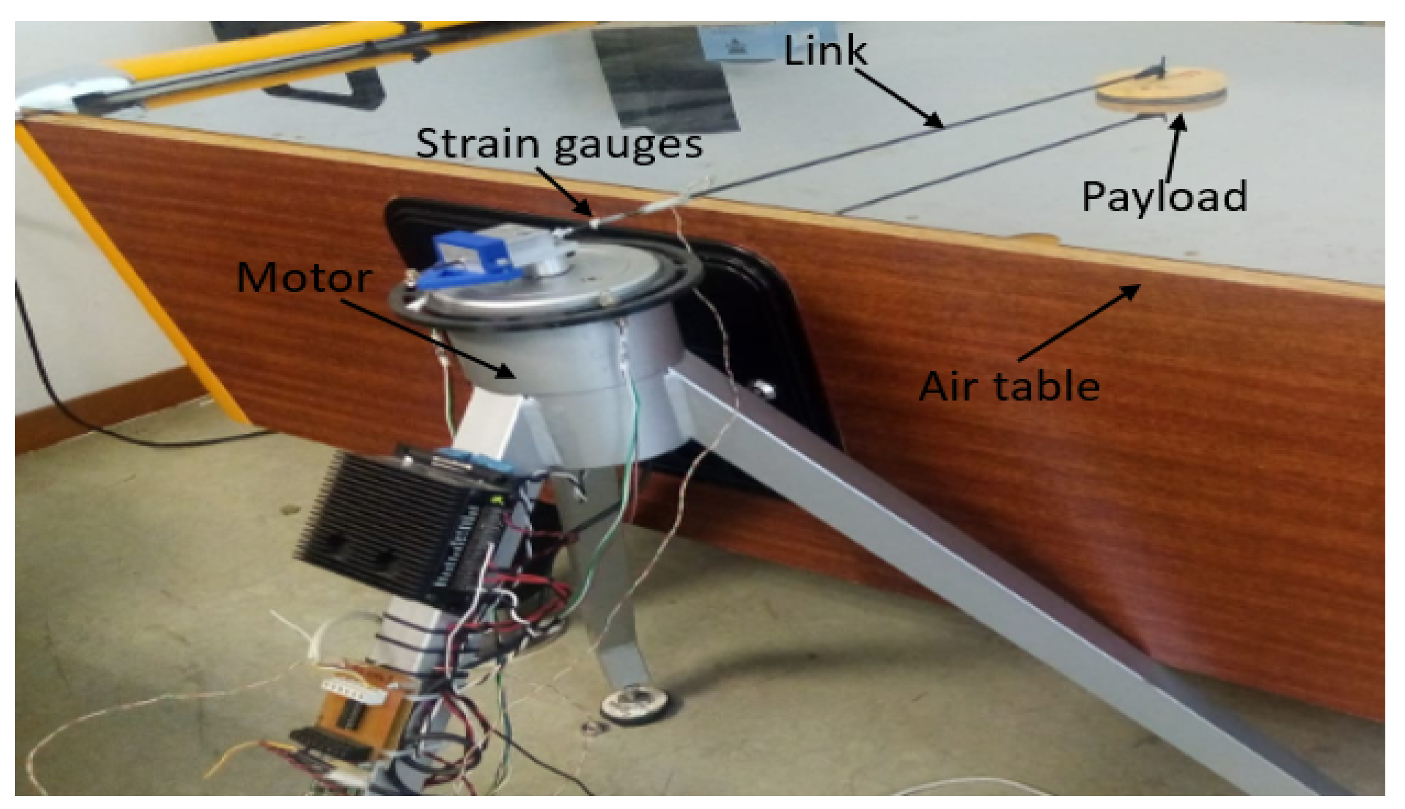
2. Experimental Setup

2.1. Flexible Robot Setup Description

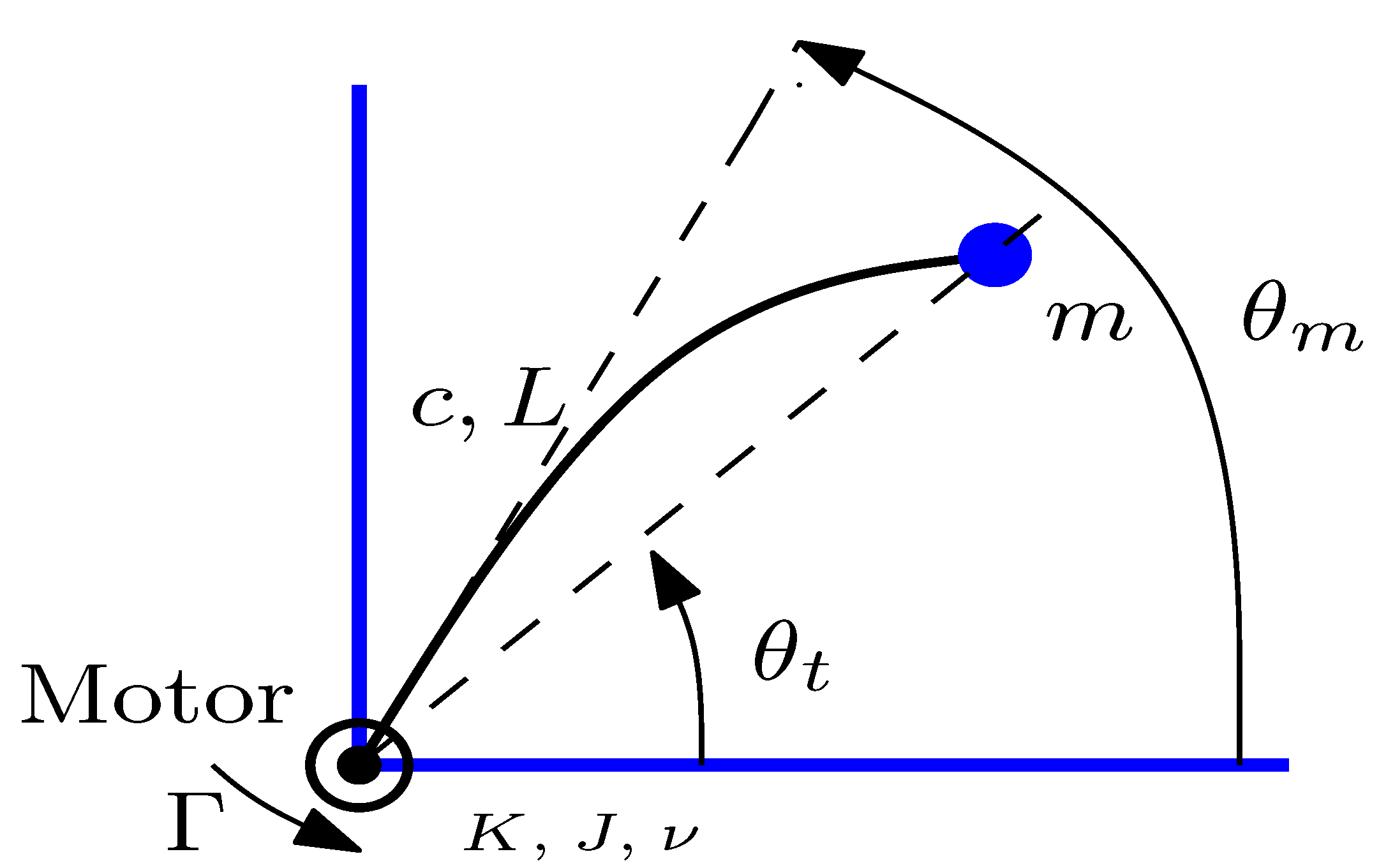
The contributions of this paper are experimentally validated in a setup located in the Robotics Laboratory at the Industrial Engineering School of the University of Castilla-La-Mancha. The setup consists of a lightweight single-link FLR mounted on an air table using a Harmonic Drive mini servo DC motor. The link is attached to the motor’s output, while a disk rotates freely at the other end of the link on an air table which helps to cancel out the gravity and friction effects. The disk serves as the payload. Both the link and the payload move in a horizontal plane, supported by the three-legged metallic structure. The FLR is equipped with an encoder in the motor for precise measurement of the motor’s angular position and a pair of strain gauges at the base of the link. Figure 1 shows this experimental platform and more details can be found in [31].

The physical parameters of the motor and of the flexible mechanism are shown in

Table 1. Values and units of the robot properties.

Symbol	Description	Numerical Values
J	Motor Inertia	$6.87·{10}^{-5}$ (kg·m${}^2$)
$\nu$	Viscous Friction	$1.041·{10}^{-3}$ (N·m·s)
K	Electromechanical Constant	0.21 (N·m·V${}^{-1}$)
L	Flexible Beam Length	0.65 (m)
$EI$	Flexural Rigidity	0.260 (N·m${}^2$)
$m_{nom}$	Nominal Tip Load	0.03 (kg)
$T_s$	Sampling Time	4 (ms)
d	Diameter	3 · 10${}^{-3}$ (m)
${\omega }_0$	Nominal Frequency	11.54 (rad·s${}^{-1}$)
${\omega }_l$	Minimal Frequency	9.42 (rad·s${}^{-1}$)
${\omega }_h$	Maximal Frequency	14.14 (rad·s${}^{-1}$)

with numerical values. The actuator of the $FLR$ is composed of three elements: a $DC$ motor, a reduction gear and a current amplifier. The actuator generates the movement of the robot following the orders received from a control unit and, hence, it actuates the rotational joint of the robot.

2.2. Robot Dynamics

Under the assumption that the distributed mass of the link is neglected and the tip mass does not induce any rotational moment at the $FLR$ tip because it can freely rotate around a vertical axis, a  lumped-mass model of the robot with a single vibration mode is defined. Figure 2 shows a scheme of this $FLR$, in which ${\theta }_m$ represents the joint angle, ${\theta }_t$ is the angle of the tip, i.e.,  the angular position of the payload, m is the payload mass placed at the end of the arm and L is the length of the link. The stiffness of the flexible link is $c=\frac{3·E·I}{L}$, where $E·I$ (N·m${}^2$) is the flexural rigidity of the link.

The dynamic model of our $FLR$ can be divided into two submodels: the first one represents the motor dynamics and the second one describes the behavior of the flexible link. These two submodels are linked by the coupling torque $\mathrm{\Gamma }$ (N·m) which is exerted between the motor and the flexible link and measured by the strain gauges placed at the base of the link.

2.2.1. Actuator Model

The actuator model connects the armature voltage to the motor angle at the gear output. It considers ${\mathrm{\Gamma }}_c$ as the Coulomb friction torque, which is a piecewise constant perturbation dependent on the sign of the motor angular velocity (explained in references [31,33]). To address the static non-linearities of the DC motor, the Coulomb friction is compensated. Additionally, the coupling torque $\mathrm{\Gamma }$ is compensated to eliminate the impact of link dynamics on the motor. These compensations are achieved by defining a fictitious input $u{}^{\prime }$ for the armature voltage, which incorporates the control signal, coupling torque and Coulomb friction. The actuator transfer function that relates the motor angle to the armature voltage fictitious input is defined by:

$$\frac{{\theta }_m\left(s\right)}{U^{\prime }\left(s\right)}=G_m\left(s\right)=\frac{K}{s·(J·s+\nu )}=\frac{A}{s·(s+B)}$$

(1)

where $A=K/J$ and $B=\nu /J$, $K(N·m/v)$ is the electromechanical constant of the motor servo-amplifier system, J (kg·m${}^2$) is the inertia of the motor and $\nu$ (N·m·s) is the viscous friction coefficient. More details about the actuator modeling are provided in [31].

2.2.2. Flexible Link Integer Order Model

The link is modeled as an Euler–Bernoulli beam with negligible distributed mass. Axial deformation is disregarded due to the presence of an air table that counteracts the effects of gravity and friction between the disk and the table surface. Since the torque at the base is a function of the second derivative of the tip position, second-order models are often used to describe the vibrations at the tip of this $FLR$. This model is derived based on the assumption of small deflections in the link, which allows us to approximate the dynamics of the $FLR$ as linear. The input to this model is the motor angle ${\theta }_m$. The dynamics of the proposed lumped-parameter model are obtained by applying Newton’s second law:

$$m·L^2·{\ddot{\theta }}_t=\mathrm{\Gamma }$$

(2)

where $\ddot{{\theta }_t}$ is the angular acceleration (rad.s${}^{-2}$) of the tip and the link deflection equation:

$$\mathrm{\Gamma }=c·({\theta }_m-{\theta }_t)$$

(3)

Combining (2) and (3) and taking Laplace transforms on the resulting equation, the transfer function between the tip and motor angles is defined by:

$$G\left(s\right)=\frac{{\theta }_t\left(s\right)}{{\theta }_m\left(s\right)}=\frac{{\varpi }^2}{s^2+{\varpi }^2}$$

(4)

where $\varpi$ is the frequency of the single vibration mode of our system, which is given by:

$$\varpi =\sqrt{\frac{c}{m·L^2}}$$

(5)

Based on Equation (4), we obtain the transfer function between the coupling torque and the motor angle assuming zero initial conditions:

$$G_{\mathrm{\Gamma }}\left(s\right)=\frac{\mathrm{\Gamma }\left(s\right)}{{\theta }_m\left(s\right)}=\frac{c·s^2}{s^2+{\varpi }^2}$$

(6)

3. Fractional Order Model of the Flexible Link

Some systems have energy diffusion phenomena that can be better modeled using fractional order differentiation. Theoretical and experimental evidence shows that this phenomenon appears in $FLR$ and is mainly associated with internal structural viscoelastic damping. As stated in the Introduction, this effect has been usually modeled by adding a damping term with a fractional order time derivative between 0 and 2 to the Euler–Bernoulli equation.

3.1. The Fractional Order Model

One main contribution of this paper is postulating a model for our $FLR$ based on the fractional generalization of Newton’s second law of motion. Then, we generalize the second-order ordinary differential equation of Newtonian mechanics by changing the order of the time derivative in the left-hand side of the Equation (2) to an arbitrary real number $\lambda$ defined in the interval $[1,2]$. This yields fractional differential equations such as the ones described in [14,34,35]. This hypothesis is supported by recent studies of physics in which second-order classical wave equations, the Schrodinger equation, the Dirac equation and several others were generalized, changing some integer order derivatives with fractional order derivatives. Then, Equation (2) becomes

$$m·L^2·D^{\lambda }{\theta }_t\left(t\right)=\mathrm{\Gamma }\left(t\right)$$

(7)

which, combined with (3) gives

$$m·L^2·D^{\lambda }{\theta }_t\left(t\right)=c·({\theta }_m\left(t\right)-{\theta }_t\left(t\right))$$

(8)

Taking Laplace transforms on this equation assuming zero initial conditions, we obtain

$$s^{\lambda }·{\theta }_t\left(s\right)+\frac{c}{m·L^2}·{\theta }_t\left(s\right)=\frac{c}{m·L^2}·{\theta }_m\left(s\right)$$

Thus,

$$G^{\lambda }\left(s\right)=\frac{{\theta }_t\left(s\right)}{{\theta }_m\left(s\right)}=\frac{{\varpi }^2}{s^{\lambda }+{\varpi }^2},\varpi =\sqrt{\frac{c}{m·L^2}}$$

(9)

and, based on this equation,

$$G_{\mathrm{\Gamma }}^{\lambda }\left(s\right)=\frac{\mathrm{\Gamma }\left(s\right)}{{\theta }_m\left(s\right)}=\frac{c·s^{\lambda }}{s^{\lambda }+{\varpi }^2}$$

(10)

Note that Equations (9) and (10) become, respectively, (4) and (6) if $\lambda =2$.

3.2. The Resonant Frequency

The resonant frequency ${\omega }_r$ is the frequency at which $\left|G^{\lambda }(j·\omega )\right|$ reaches its maximum value. Then, the frequency response of (9) is obtained taking into account that ${(j·\omega )}^{\lambda }={\omega }^{\lambda }·e^{j·\frac{\pi }{2}·\lambda }={\omega }^{\lambda }·\left(\cos (\frac{\pi }{2}·\lambda )+j·\sin (\frac{\pi }{2}·\lambda )\right)$:

$$G^{\lambda }(j·\omega )=\frac{{\varpi }^2}{{\omega }^{\lambda }·\left(\cos \left(\frac{\pi }{2}·\lambda \right)+j·\sin \left(\frac{\pi }{2}·\lambda \right)\right)+{\varpi }^2}$$

(11)

Let us represent by $f\left(\omega \right)$ the denominator of this equation. Then, the module squared of this function is:

$${\left|f\left(\omega \right)\right|}^2={\left(\cos \left(\frac{\pi }{2}·\lambda \right)·{\omega }^{\lambda }+{\varpi }^2\right)}^2+{\sin }^2\left(\frac{\pi }{2}·\lambda \right)·{\omega }^{2·\lambda }$$

(12)

Equating to zero the derivative of ${\left|f\left(\omega \right)\right|}^2$ with respect to $\omega$ yields

$$\frac{{\partial \left|f\left(\omega \right)\right|}^2}{\partial \omega }={\omega }^{\lambda }+{\varpi }^2·\cos \left(\frac{\pi }{2}·\lambda \right)=0$$

(13)

from which we obtain

$${\omega }_r={\left(-{\varpi }^2·\cos \left(\frac{\pi }{2}·\lambda \right)\right)}^{\frac{1}{\lambda }}$$

(14)

This expression shows that if $0<\lambda \le 1$ then the resonant frequency ${\omega }_r$ does not exist.

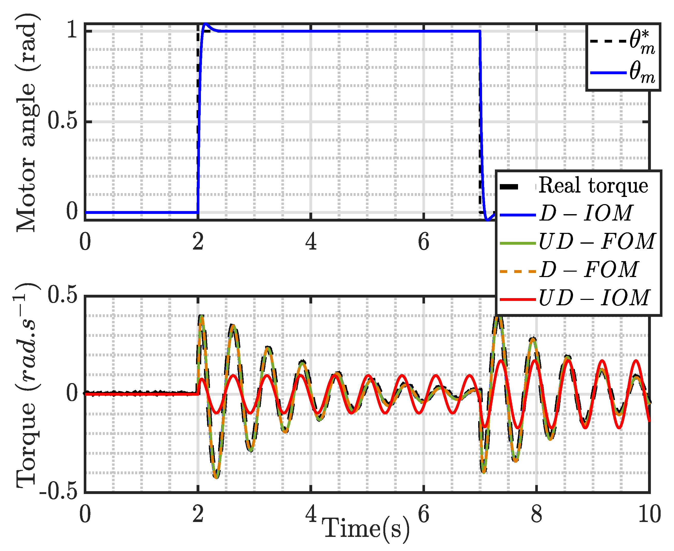
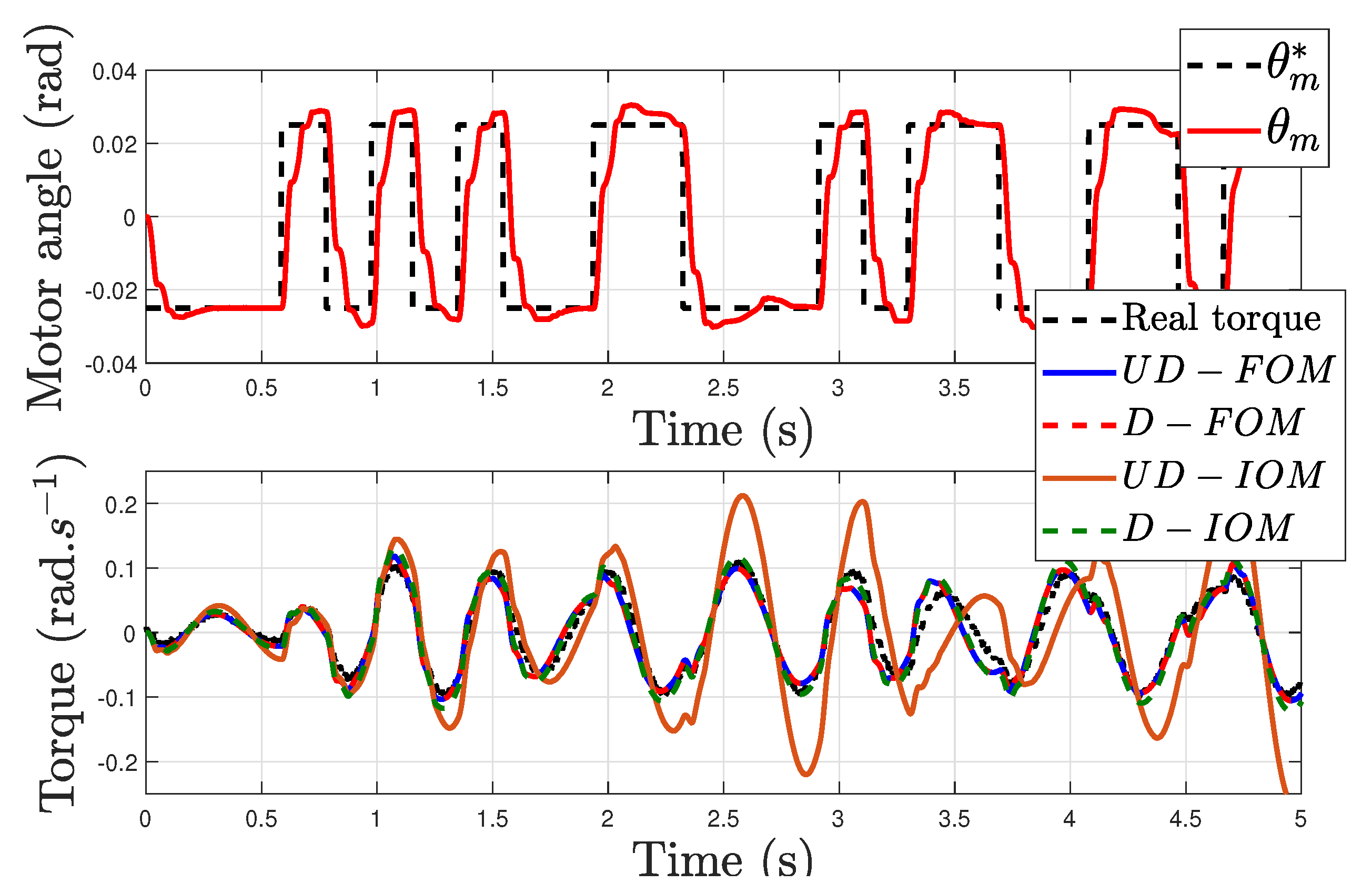
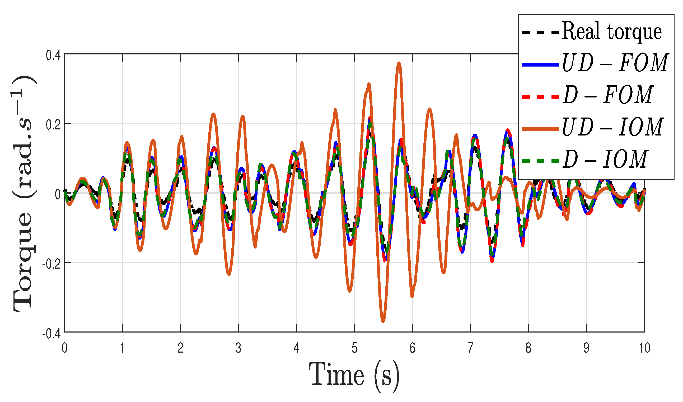
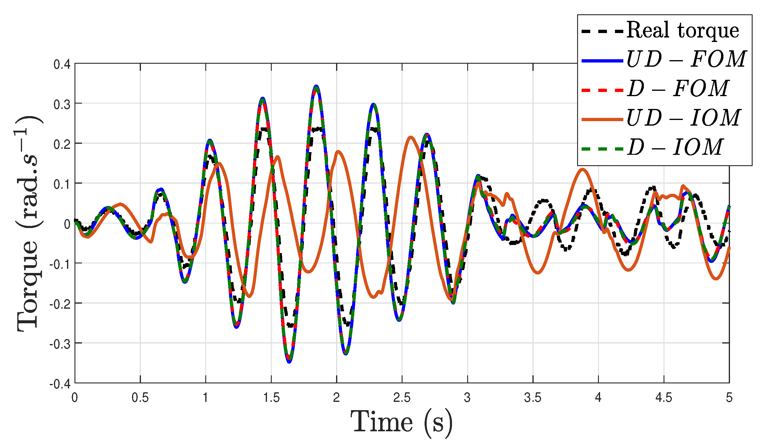
3.3. Experimental Validation of the Dynamic Model

In this subsection, experiments justify the interest of the proposed model and the use of a constant fractional order $\lambda$ that does not depend on payload changes. This is carried out by comparing the fitting to experimental data obtained from the motor encoder and the strain gauges of (1) the undamped integer order model ($UD$-$IOM$) given in (6), (2) the damped integer order model (D-$IOM$) given by

$$G_{\mathrm{\Gamma }}\left(s\right)=\frac{\mathrm{\Gamma }\left(s\right)}{{\theta }_m\left(s\right)}=\frac{c·s^2}{s^2+\mu ·s+{\varpi }^2}$$

(15)

(3) the integer order model with fractional order damping (D-$FOM$) given by

$$G_{\mathrm{\Gamma }}\left(s\right)=\frac{\mathrm{\Gamma }\left(s\right)}{{\theta }_m\left(s\right)}=\frac{c·s^2}{s^2+\mu ·s^{\alpha }+{\varpi }^2}$$

(16)

and (4) the fractional order model ($UD$-$FOM$) given in (10).

As a first step, the parameters of these four models are identified from collected data of the motor angle ${\theta }_m$ and the coupling torque $\mathrm{\Gamma }$. The model is identified using the previous experimental measures, the Matlab software and the Mean Square Error ($MSE$) as the fitting function to be minimized. The identification method is presented in Algorithm 1:

Algorithm 1 Model-based identification system algorithm

1. Collect experimental input–output data that represent the system’s behavior to be modeled. 2. Define transfer function structure. 3. Create an initial model using the transfer function with arbitrary coefficients. 4. Estimate the model parameters using optimization in Matlab to estimate the model parameters based on the data collected in step 1. 5. Evaluate the model obtained by computing the $MSE$ which is the mean square of the difference between the predicted output of the system defined by $\widehat{y}$ and the experimental output defined by y. 6. if $MSE>{ϵ}_m$ ($\widehat{y}$ is different from y) then     Repeat steps 4 and 5 until an acceptable level of accuracy is obtained (the value of the $MSE$ is under the threshold ${ϵ}_m$). end if

The trajectory of ${\theta }_m\left(t\right)$ used to identify the dynamic models is a pulse signal 7 s wide with an amplitude of 1 $\mathrm{rad}$. The pulse signal has a wide frequency content that excites the system at different frequencies and its impulse-like shape allows for a straightforward analysis of the system’s response. Hence, for this trajectory, ${\theta }_m\left(t\right)$, the $MSE$ existing between the experimental torque $\mathrm{\Gamma }\left(t\right)$ and the coupling torque responses predicted via the four fitted models are $0.058$ with $UD$-$IOM$, $0.00531$ with D-$IOM$, $0.00524$ with D-$FOM$ and $0.00524$ with $UD$-$FOM$. This means that introducing a fractional order derivative on the model of our $FLR$ to account for the damping reduces the $MSE$ of the standard second-order undamped model in $91.21\%$. Figure 3 presents the motor angle trajectory, the measured coupling torque and the coupling torque responses predicted via these four identified models. The proposed model is clearly able to introduce a damping behavior in the $FLR$. This model is more valuable and less complicated than an integer order model with a damping factor.

Table 2. Parameters of the Predicted Models.

	$\mathit{\alpha }$	$\mathit{\lambda }$	$\mathit{\mu }$	$\mathit{\varpi }$	$\mathit{MSE}$	$\mathit{AIC}(·{10}^4$)
UD-IOM	xx	2.00	xx	10.20	0.05845	−1.4199
D-IOM	xx	2.00	1.30	10.20	0.00531	−2.6192
UD-FOM	xx	1.92	xx	10.02	0.00524	−2.6258
D-FOM	0.9	2.00	1.37	10.50	0.00524	−2.6256

highlights that there is a significant difference in the $MSE$ assessed from the response of the $UD$-$IOM$ model and the rest: the error obtained from the first model is 10 times greater than the error of the rest of the models. The $MSE$ has the same value for the $UD$-$FOM$ and D-$FOM$. At this level, we introduce another criterion in order to evaluate the model quality. Accordingly, the $AIC$, which stands for Akaike Information Criterion, is needed to choose between the $UD$-$FOM$ and D-$FOM$ models as an additional selective indicator. It measures the relative quality of a model for a given set of data. It balances the goodness of fit of a model with the number of parameters used to define the model, penalizing models that are too complex and giving preference to models that fit the data well with fewer parameters. In the case of a huge number of observations (samples) n, its expression is

$$AIC=2·k-2·\log \left(Lik\right)$$

(17)

where k is the number of parameters in the model and $Lik$ is the likelihood function. Expression (17) can be written in terms of the $MSE$ as:

$$AIC=2·k+n·\log \left(MSE\right)$$

(18)

In general, a lower $AIC$ score is better. Therefore, when comparing different models, the model with the lowest $AIC$ score is usually considered the best among the candidate models.

The estimated parameters obtained from the identification process of the four dynamic models presented, respectively, in (6), (10), (15) and (16) are summarized in Table 2, which also includes the performance indicators. Parameter $c=1.56$ N·m was obtained via direct experimentation and we assume that it is constant in all present and future experiments. It can be concluded that the D-$FOM$ and the $UD$-$FOM$ have the lowest $MSE$ but this last one has only two parameters to be tuned ($\lambda$, $\varpi$), while the previous one has three ($\alpha$, $\mu$, $\varpi$). The D-$IOM$ has two parameters to be tuned ($\mu$, $\varpi$) like the $UD$-$FOM$, but it has an $MSE$ slightly higher than the $UD$-$FOM$. Moreover, this last model has a lower $AIC$ score compared to the D-$FOM$ model, so it achieves a similar fit while using fewer parameters. All this is translated to the fact that the $UD$-$FOM$ proposed in this paper has the lowest $AIC$ value and, then, it is the most accurate model that, moreover, has the fewest parameters, i.e., is the simplest model.

As a second step, we will prove that the fractional parameter $\lambda$ of the identified $UD$-$FOM$ model is invariant with respect to payload changes. Figure 4, Figure 5 and Figure 6 compare the real and the predicted coupling torques for several values of the tip mass when integer and fractional order models are used. The system is excited by a Pseudo-Random Binary Sequence ($PRBS$) signal. This kind of signal ensures that the system is excited at a broad range of frequencies and amplitudes, allowing a more comprehensive analysis of the system’s behavior over time. The real torque in Figure 4 presents a resonant frequency ${\omega }_{r,nom}=11.86$ rad·s${}^{-1}$ for the nominal payload ($m_{nom}=30$ g). The real torque used in Figure 5 presents a resonant frequency ${\omega }_{r,min}=10.68$ rad·s${}^{-1}$ for the maximal payload ($m_{max}=40$ g). The real torque in Figure 6 presents a resonant frequency ${\omega }_{r,max}=14.93$ rad·s${}^{-1}$ for the minimal payload ($m_{min}=20$ g). The parameters of the damped systems (D-$FOM$ and D-$IOM$) $\alpha$ and $\mu$ are considered constant for the three payload cases and are identified jointly for the three experiments in such a way that they give the minimum value of the sum of the $MSE$ in the three payload cases. Then, $\alpha$ = 0.954 and $\mu$ = 1.37 were obtained.

The features of the three estimated torques are shown in

Table 3. Features of the Predicted Models in the Different Payload Changes.

		$\mathit{UD}$-$\mathit{FOM}$	D-$\mathit{FOM}$	$\mathit{UD}$-$\mathit{IOM}$	D-$\mathit{IOM}$
$m_{min}$	$\varpi$	$14.749$	$14.881$	$10.22$	$15.012$
	$\lambda$	$1.92$	2	2	2
	$MSE$	$0.00708$	$0.00719$	$0.150182$	$0.0072$
$m_{nom}$	$\varpi$	$10.311$	$12.2426$	$11.4142$	$11.5179$
	$\lambda$	$1.92$	2	2	2
	$MSE$	$0.01662$	$0.01664$	$0.0742$	$0.016715$
$m_{max}$	$\varpi$	$10.2402$	$11.501$	$11.6735$	$11.251$
	$\lambda$	$1.92$	2	2	2
	$MSE$	$0.0207$	$0.0213$	$0.0772$	$0.0211$

and with that table we can see that:

• The $FO$ of the identified $UD$-$FOM$ is kept constant during the payload changes, with a value $\lambda =1.92$.
• The frequency $\varpi$ changes significantly with the payload, in accordance with expression (5).
• The $UD$-$FOM$ models have the lowest $MSE$ compared to the rest of the models.

Finally, we remark that the identified natural frequencies $\varpi$ are close but not equal to the resonant frequencies ${\omega }_r$ obtained experimentally, because the damping coefficient or the fractional orders influence their relationship (see, e.g., ref. (14) for the case of $UD$-$FOM$).

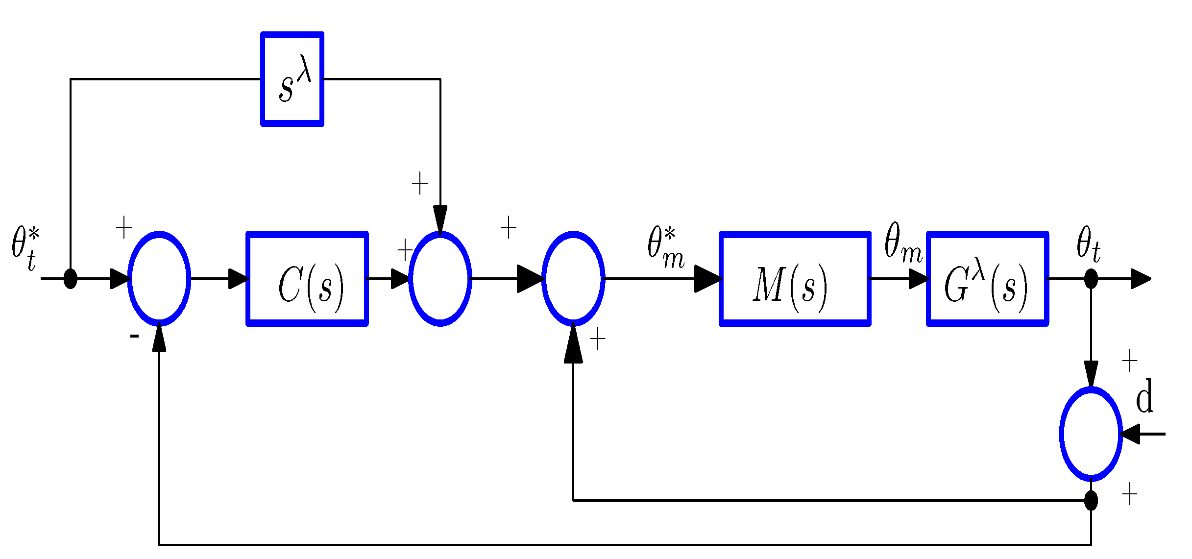
4. General Control Scheme

The control system presented in this work incorporates a feedback mechanism using the angle of the actuator, denoted ${\theta }_m$, and the moment at the base of the link, denoted $\mathrm{\Gamma }$. This control scheme, outlined and described in detail in the references [33,36], involves a nested structure consisting of two control loops based on the motor angle and the coupling torque:

• The inner loop employs the measured motor angle, ${\theta }_m$, to regulate the motor position. It effectively gets out the effects of non-linear Coulomb friction and time-varying viscous friction. Moreover, in order to ensure a faster dynamic response of the servo-controlled motor compared to the flexible link, this inner loop was implemented with a high-gain controller.
• The outer loop focuses on controlling the position of the payload at the tip to mitigate the occurrence of mechanical vibrations and ensure good trajectory tracking.

The control scheme presented here entails the use of the outer loop’s control law output as a reference for the inner loop, splitting the control system design into two stages. The motor is then controlled in a manner that maximizes its response rapidity within the limits of saturation levels. To address the design of the outer loop, the singular perturbation theory is employed, which allows us to neglect the inner loop dynamics in the case that it is sufficiently fast. Subsequently, the outer loop controller is tuned to achieve the wanted performance related to the positioning of the tip. Both control loops are then merged into a singularly perturbed model and a stability analysis of the closed-loop plant is conducted.

4.1. The Inner Loop

The control scheme described in [36] is currently employed in this work. It is a robust controller based on two-degree-of-freedom $PID$s. It incorporates a feedback term in order to compensate for the coupling torque—which makes the controlled motor dynamics less affected by the motion of the link—and mitigate the impact of Coulomb friction. This feedback term simplifies the motor model used in the controller design.

Hence, based on this simplified model, a two-degree-of-freedom $PID$ control scheme is designed, as depicted in Figure 7. The control scheme consists of two $PID$ controllers that incorporate a low-pass filter:

$$C_{m1}\left(s\right)=\frac{a_2·s^2+a_1·s+a_0}{s·(s+c)}$$

(19)

$$C_{m2}\left(s\right)=\frac{b_1·s+b_0}{s+c}$$

(20)

According to the method outlined in [32], a pole-placement technique is implemented. The four poles of the closed-loop system are located at the same position, denoted z. Additionally, the two zeros are also positioned at z. As a result, two out of the four poles are eliminated by the two zeros, which gives the simplified closed-loop transfer function:

$$\frac{{\theta }_m\left(s\right)}{{\theta }_m^{*}\left(s\right)}=M\left(s\right)=\frac{1}{{(1+ϵ·s)}^2},ϵ=-\frac{1}{z}$$

(21)

By employing this control mechanism, precise trajectory tracking and rapid motor positioning are assured through effective compensation for disturbances such as unmodeled friction components and robustness against motor parameter uncertainties. To achieve very fast motor movements, a high value for $\left|z\right|$ is selected, i.e., a small $ϵ$ is looked for.

4.2. The Outer Loop

In order to remove vibrations in the flexible link, an outer control loop is designed by combining the input-state linearization technique and singular perturbation theory. The nonlinear controller proposed in [36] for a haptic device was adapted to suit our 1-DOF linear flexible link robot. By applying the principles of singular perturbation theory, the controller was initially designed assuming $M\left(s\right)=1$ and, then, the stability of the closed-loop system including (21) was assessed.

The system to be controlled is characterized by the transfer function $G\left(s\right)$ as given in Equation (9). By considering Figure 8 and employing the input-state linearization technique to $G\left(s\right)$, the control law obtained is:

$${\theta }_m^{*}\left(s\right)={\theta }_t^{*}\left(s\right)+\left(s^{\lambda }·{\theta }_t^{*}\left(s\right)+C\left(s\right)·\left({\theta }_t^{*}\left(s\right)-{\theta }_t\left(s\right)\right)\right)$$

(22)

In this context, ${\theta }_t^{}\left(s\right)$ corresponds to the intended trajectory of the manipulator, ${\theta }_m^{}\left(s\right)$ denotes the control signal produced by the outer loop that acts as the reference for the enclosed loop and $C\left(s\right)$ represents the controller used in the outer loop.

In Figure 8, ${\theta }_t$ is estimated using measurements of ${\theta }_m$ and $\mathrm{\Gamma }$. Specifically, ${\theta }_t$ is calculated as mentioned in Equation (3), which gives ${\theta }_t\left(t\right)={\theta }_m\left(t\right)-\frac{\mathrm{\Gamma }\left(t\right)}{c}$. If the measurements of the coupling torque were affected by a disturbance $d^{\prime }\left(t\right)$, this would yield a modified estimated moment value ${\mathrm{\Gamma }}^e\left(t\right)=\mathrm{\Gamma }\left(t\right)+d^{\prime }\left(t\right)$. Consequently, the estimated value of ${\theta }_t$ would be modified, becoming:

$${\theta }_t^e\left(t\right)={\theta }_m\left(t\right)-\frac{{\mathrm{\Gamma }}^e\left(t\right)}{c}={\theta }_m\left(t\right)-\frac{\mathrm{\Gamma }\left(t\right)}{c}+d\left(t\right)$$

(23)

Representing the disturbance in the estimation of the tip position as $d\left(t\right)=-\frac{d^{\prime }\left(t\right)}{c}$, Figure 8 depicts the structure of our control system with the presence of this sensor disturbance.

After performing certain operations, the transfer matrix that establishes the relationship between ${\theta }_t\left(t\right)$ and ${\theta }_m^{*}\left(t\right)$ with ${\theta }_t^{*}\left(t\right)$ and $d\left(t\right)$ is determined:

$$\left(\begin{array}{c}{\theta }_t\left(s\right)\\ {\theta }_m^{*}\left(s\right)\end{array}\right)=\frac{\left(\begin{array}{cc}M\left(s\right)·G^{\lambda }\left(s\right)·\left(C\left(s\right)+s^{\lambda }\right)& -M\left(s\right)·G^{\lambda }\left(s\right)·\left(C\left(s\right)-1\right)\\ C\left(s\right)+s^{\lambda }& -C\left(s\right)+1\end{array}\right)}{1+M\left(s\right)·G^{\lambda }\left(s\right)·\left(C\left(s\right)-1\right)}·\left(\begin{array}{c}{\theta }_t^{*}\left(s\right)\\ d\left(s\right)\end{array}\right)$$

(24)

and substituting $G^{\lambda }\left(s\right)$ by its expression defined in (9) into this,

$$\left(\begin{array}{c}{\theta }_t\left(s\right)\\ {\theta }_m^{*}\left(s\right)\end{array}\right)=\underset{P\left(s\right)}{\underbrace{\frac{\left(\begin{array}{cc}{\varpi }^2·M\left(s\right)·\left(C\left(s\right)+s^{\lambda }\right)& -{\varpi }^2·M\left(s\right)·\left(C\left(s\right)-1\right)\\ \left(C\left(s\right)+s^{\lambda }\right)·\left({\varpi }^2+s^{\lambda }\right)& -\left(C\left(s\right)-1\right)·\left({\varpi }^2+s^{\lambda }\right)\end{array}\right)}{s^{\lambda }+{\varpi }^2+{\varpi }^2·M\left(s\right)·\left(C\left(s\right)-1\right)}}}·\left(\begin{array}{c}{\theta }_t^{*}\left(s\right)\\ d\left(s\right)\end{array}\right)$$

(25)

The sensors used to measure the vibrations in the experimental platform are strain gauges [37]. They are often used in robotic systems due to several advantages that make them highly recommended in applications. Their main advantages are recapitulated in the following: (1) they enable the measurement of vibrational signals as well as deflections, (2) they are easily implemented and used and can be reusable and (3) they are relatively low cost. However, strain gauges have several drawbacks [11,36], such as: (1) huge temperature variations, (2) high-frequency noise capable of saturating the actuators and (3) offset, which leads to a steady-state error that affects the end position of the link [38]. These drawbacks will be addressed in the next section.

5. Control Robust to Strain Gauge Disturbances

Good trajectory tracking is a pledge of an efficient $FLR$ controller. Therefore, some external and internal conditions should be taken into consideration when designing this control such as its ability to remove sensor disturbances such as the offset and the high-frequency noise [36] and its robustness to payload changes.

5.1. Strain Gauge Offset Disturbance Removal

Take into account the transfer function presented in Equation (25), which establishes the relationship between ${\theta }_t\left(s\right)$ and $d\left(s\right)$:

$$\frac{{\theta }_t\left(s\right)}{d\left(s\right)}=P_{1,2}\left(s\right)=-\frac{{\varpi }^2·M\left(s\right)·\left(C\left(s\right)-1\right)}{s^{\lambda }+{\varpi }^2+{\varpi }^2·M\left(s\right)·\left(C\left(s\right)-1\right)}$$

(26)

As the offset can be represented as a step disturbance $d\left(s\right)=\frac{\widehat{d}}{s}$, the steady state error $e_{{\theta }_t}$ induced in ${\theta }_t$ can be assessed by applying the final value theorem:

$$e_{{\theta }_t}=\underset{s\to 0}{lim}s·P_{1,2}\left(s\right)·d\left(s\right)=-{\omega }^2·\frac{M\left(0\right)·\left(C\left(0\right)-1\right)}{{\varpi }^2+{\varpi }^2·M\left(0\right)·\left(C\left(0\right)-1\right)}·\widehat{d}$$

(27)

Considering that $M\left(0\right)=1$, the aforementioned equation indicates that $C\left(0\right)$ must be adjusted to a value of 1 to ensure that $e_{{\theta }_t}$ becomes zero. Therefore, the controller structure should take the following form:

$$C\left(s\right)=\widehat{C}\left(s\right)+1,\widehat{C}\left(0\right)=0$$

(28)

This implies that $\widehat{C}\left(s\right)$ should have a zero at the origin to effectively eliminate the steady-state error caused by the offset of the strain gauges.

5.2. High-Frequency Noise Reduction

We represent the sensor noise by an unbiased high-frequency noise with an unknown statistical description, as was described in [39] from a relatively recent and non-standard analysis viewpoint. Then, this noise has a spectrum located at the highest frequency zone.

The control signal ${\theta }_m^{*}\left(t\right)$ is susceptible to amplified noise due to high-frequency noise in the sensor, which can result in actuator saturation, which ultimately leads to the rise of insufficient dynamic performance and potential instability. Let us examine the transfer function given in Equation (25), which establishes the relationship between ${\theta }_m^{*}\left(s\right)$ and $d\left(s\right)$:

$$\frac{{\theta }_m^{*}\left(s\right)}{d\left(s\right)}=P_{2,2}\left(s\right)=-\frac{\left(C\left(s\right)-1\right)·\left({\varpi }^2+s^{\lambda }\right)}{s^{\lambda }+{\varpi }^2+{\varpi }^2·M\left(s\right)·\left(C\left(s\right)-1\right)}$$

(29)

By considering a controller in the form of Equation (28), we can deduce that:

$$P_{2,2}\left(s\right)=-\frac{\widehat{C}\left(s\right)·\left({\varpi }^2+s^{\lambda }\right)}{s^{\lambda }+{\varpi }^2·(1+M\left(s\right)·\widehat{C}\left(s\right))}$$

(30)

Assuming that the high-frequency noise in the strain gauge signal is represented by a sinusoidal signal with a significantly high frequency, the frequency response of $P_{2,2}$ as $\omega \to \infty$ demonstrates the impact of the amplification of this noise on the control signal ${\theta }_m^{*}$ of the outer loop. To further analyze this behavior, we divide the numerator and denominator of $P_{2,2}\left(s\right)$ by $s^{\lambda }$ resulting in:

$$\underset{\omega \to \infty }{lim}\left|P_{2,2}(j·\omega )\right|=\underset{\omega \to \infty }{lim}\frac{|\widehat{C}(j·\omega )|·\left|1+\frac{{\varpi }^2·e^{-j·\frac{\pi }{2}·\lambda }}{{\omega }^{\lambda }}\right|}{\left|1+{\varpi }^2·e^{-j·\frac{\pi }{2}·\lambda }·\left(\frac{1}{{\omega }^{\lambda }}+\frac{M(j·\omega )·\widehat{C}(j·\omega )}{{\omega }^{\lambda }}\right)\right|}$$

(31)

Assuming that

$$\underset{\omega \to \infty }{lim}\left|\widehat{C}(j·\omega )\right|=0$$

(32)

it is easy to prove that expression (31) becomes ${lim}_{\omega \to \infty }\left|P_{2,2}(j·\omega )\right|=0$. Then, the impact of a high-frequency noise component of the signal ${\theta }_m^{*}\left(t\right)$ can be significantly diminished if condition (32) is verified. This condition involves that $\widehat{C}\left(s\right)$ must be strictly proper. However, since high gains are used to close the inner loop, the influence of ${\theta }_m^{*}\left(t\right)$ high-frequency noise on the motor input is significantly amplified. As a result, the motor is prone to saturation. To avoid this undesirable effect, it is crucial to guarantee that condition (32) is satisfied.

6. Control Robust to Payload Changes

Variations in the payload mass m directly impact the natural vibration frequency $\varpi$, as expressed in Equation (9). These changes in frequency can potentially lead to underdamped or unstable closed-loop systems. To address this issue, this section focuses on the development of a controller $C\left(s\right)$ to be incorporated in the control system shown in Figure 8 which enhances the robustness to payload changes. Additionally, the controller should exhibit robustness to the two disturbances studied in the previous section. Then, conditions (28) and (32) must be verified.

Based on the $FO$ model defined in Equation (9), the first path of the Nyquist diagram (indicated in Figure 9 in brown color) corresponds to the frequency response of $G^{\lambda }\left(s\right)$, where $\omega$ is defined in the interval $0<\omega <\infty$. This plot shows that the system exhibits a small positive phase margin. Therefore, though the closed-loop system is stable, its phase margin has to be increased in order to improve the damping. It can be achieved by designing a phase lead controller $\widehat{C}\left(s\right)$. Let us assume that such a controller is an $FO$ derivative controller:

$$\widehat{C}\left(s\right)=k_d·s^{\beta },0<\beta <2$$

(33)

The $FO$ operator $s^{\beta }$ is often approximated numerically. We use in this paper the Grünwald–Letnikov definition based on the backward difference.

The evident simplest choice for (33) is the classical integer order derivative controller, which is obtained by making $\beta =1$ in this expression. It verifies that $\widehat{C}\left(0\right)=0$ and can improve the damping of the closed-loop system $\zeta$ by increasing its phase margin ${\varphi }_m$ in $\frac{\pi }{2}$ rads. However, we cannot achieve desired closed-loop settling time $t_s$ because we can only tune one parameter, $k_d$, in this structure. Then, we tune the two parameters $\beta >0$ and $k_d$ of controller (33) by using a frequency domain technique and the following approximate relations: ${\varphi }_m\approx 100\zeta$—which is an expression originally developed for second order systems (e.g., ref. [40])—and $t_s\approx 2\pi /{\omega }_c$.

The blue line of Figure 9 represents the first path of the Nyquist diagram of the open-loop transfer function of the controlled system:

$$L(j·\omega ,\varpi )=\widehat{C}(j·\omega )·G^{\lambda }(j·\omega ,\varpi )=k_d·{(j·\omega )}^{\beta }·\frac{{\varpi }^2}{{(j·\omega )}^{\lambda }+{\varpi }^2}$$

(34)

in which the dependence on $\varpi$ has been made explicit in $L\left(\right)$ and $G^{\lambda }\left(\right)$. The gain crossover frequency ${\omega }_c$ and the phase margin ${\varphi }_m$ are highlighted in this plot. According to this diagram, the control system is designed such that ${\omega }_c>{\omega }_r$. Next, we develop some results useful for designing a control system robust to payload changes.

Lemma 1.

Consider the frequency response $L(j·\omega ,\varpi )$ given by (34). Its phase is a decreasing function with ω that decreases from $\frac{\pi }{2}·\beta$ rads to $\frac{\pi }{2}·\left(\beta -\lambda \right)$ rads. Moreover, changes in the value of ϖ only produce a homothety of the Nyquist plot of $L(j·\omega ,\varpi )$ with the center in the origin.

Proof. 

The phase of (34) is

$$arg\left(L(j·\omega ,\varpi )\right)=\frac{\pi }{2}·\beta -\arctan \left(\frac{\sin \left(\frac{\pi }{2}·\lambda \right)·{\omega }^{\lambda }}{\cos \left(\frac{\pi }{2}·\lambda \right)·{\omega }^{\lambda }+{\varpi }^2}\right)$$

(35)

Differentiating this expression with respect to $\omega$ yields

$$\frac{\partial arg\left(L(j·\omega ,\varpi )\right)}{\partial \omega }=-\frac{\lambda ·{\varpi }^2·\sin \left(\frac{\pi }{2}·\lambda \right)·{\omega }^{\lambda -1}}{{\omega }^{2·\lambda }+2·{\varpi }^2·\cos \left(\frac{\pi }{2}·\lambda \right)·{\omega }^{\lambda }+{\varpi }^4}$$

(36)

Since $1<\lambda \le 2$, we have that $\cos (\frac{\pi }{2}·\lambda )\le 0$ and $\sin (\frac{\pi }{2}·\lambda )\ge 0$. Then, the numerator of (36) is positive and, taking into account that

$${\omega }^{2·\lambda }+2·{\varpi }^2·\cos \left(\frac{\pi }{2}·\lambda \right)·{\omega }^{\lambda }+{\varpi }^4\ge {\omega }^{2·\lambda }-2·{\varpi }^2·{\omega }^{\lambda }+{\varpi }^4={\left({\omega }^{\lambda }-{\varpi }^2\right)}^2\ge 0$$

(37)

its denominator is also positive. Then, $\frac{\partial arg\left(L(j·\omega ,\varpi )\right)}{\partial \omega }<0$, i.e., the phase of $L(j·\omega ,\varpi )$ is a decreasing function with $\omega$. The range of variation of $arg\left(L(j·\omega ,\varpi )\right)$ is easily obtained from (35) by making the limits of $arg\left(L(j·\omega ,\varpi )\right)$ when $\omega \to 0$ and $\omega \to \infty$.

Moreover, expression (34) can be written for $x=\omega /{\varpi }^{\frac{2}{\lambda }}$ as

$$L(j·x,\varpi )=k_d·{\varpi }^{\frac{2·\beta }{\lambda }}{(j·x)}^{\beta }·\frac{1}{{(j·x)}^{\lambda }+1}$$

(38)

which illustrates that the shape of $L(j·\omega ,\varpi )$ is the same for any $\varpi$ and, in this expression, variations of $\varpi$ only produce changes in the scaling factor ${\varpi }^{\frac{2·\beta }{\lambda }}$. □

Theorem 1.

For a given controller $\widehat{C}(j·\omega )$ of the form (33), the phase margin of the open-loop transfer function (34) is non increasing with ϖ, i.e., $\frac{d{\varphi }_m}{d\varpi }\le 0$, if it is verified that $1<\lambda \le 2$, $0<\beta <\lambda$ and

$${\omega }_c>{\left(\frac{-{\varpi }^2}{cos\left(\frac{\pi }{2}·\lambda \right)}\right)}^{\frac{1}{\lambda }}$$

(39)

Proof. 

First of all, note that condition (39) is the same as

$${\varpi }^2+\cos \left(\frac{\pi }{2}·\lambda \right)·{\omega }_c^{\lambda }<0$$

(40)

and, taking into account that $\lambda >1$, this inequality implies that

$$0<\frac{{\varpi }^2}{\cos \left(\frac{\pi }{2}·\lambda \right)}+{\omega }_c^{\lambda }\le \cos \left(\frac{\pi }{2}·\lambda \right)·{\varpi }^2+{\omega }_c^{\lambda }$$

(41)

Next, assume the open-loop frequency response (34). The relationship among its phase margin ${\varphi }_m$, its gain crossover frequency ${\omega }_c$ and its natural frequency $\varpi$, is given by, e.g., ref. [41]:

$$k_d·{(j·{\omega }_c)}^{\beta }·\frac{{\varpi }^2}{{(j·{\omega }_c)}^{\lambda }+{\varpi }^2}=-e^{j·{\varphi }_m}$$

(42)

Equating magnitudes in this expression and squaring yields

$$k_d^2·{\omega }_c^{2·\beta }·{\varpi }^4={\omega }_c^{2·\lambda }+2·\cos \left(\frac{\pi }{2}·\lambda \right)·{\varpi }^2·{\omega }_c^{\lambda }+{\varpi }^4$$

(43)

and equating phases

$$\frac{\pi }{2}·\beta +\pi -\arctan \left(\frac{\sin \left(\frac{\pi }{2}·\lambda \right)·{\omega }^{\lambda }}{\cos \left(\frac{\pi }{2}·\lambda \right)·{\omega }^{\lambda }+{\varpi }^2}\right)={\varphi }_m$$

(44)

Differentiating expression (44) with respect to $\varpi$ (note that $\varpi$ and $\omega$ are linked by (43)), we obtain that

$$\frac{d{\varphi }_m}{d\varpi }=-\sin \left(\frac{\pi }{2}·\lambda \right)·\varpi ·{\omega }_c^{\lambda -1}·\frac{\lambda ·\varpi ·\frac{d{\omega }_c}{d\varpi }-2·{\omega }_c}{{\omega }_c^{2·\lambda }+2·\cos \left(\frac{\pi }{2}·\lambda \right)·{\varpi }^2·{\omega }_c^{\lambda }+{\varpi }^4}$$

(45)

Differentiating expression (43) with respect to $\varpi$ and ${\omega }_c$, we obtain that

$$\begin{array}{c}\hfill 2·\left(\left(k_d^2·{\omega }_c^{2·\beta }-1\right)·{\varpi }^3-\cos \left(\frac{\pi }{2}·\lambda \right)·\varpi ·{\omega }_c^{\lambda }\right)·d\varpi +\hfill \\ \hfill \left(\beta ·k_d^2·{\varpi }^4·{\omega }_c^{2·\beta -1}-\lambda ·\cos \left(\frac{\pi }{2}·\lambda \right)·{\varpi }^2·{\omega }_c^{\lambda -1}-\lambda ·{\omega }_c^{2·\lambda -1}\right)·d{\omega }_c=0\hfill \end{array}$$

(46)

Substituting (43) in the first and second terms of the left side member of (46) and operating yields

$$\begin{array}{c}2·\frac{{\omega }_c^{\lambda }}{\varpi }·\left({\omega }_c^{\lambda }+{\varpi }^2·\cos \left(\frac{\pi }{2}·\lambda \right)\right)·d\varpi +\hfill \\ \frac{1}{{\omega }_c}·\left(-\left(\lambda -\beta \right)·{\omega }_c^{\lambda }·\left({\omega }_c^{\lambda }+\cos \left(\frac{\pi }{2}·\lambda \right)·{\varpi }^2\right)+\beta ·{\varpi }^2·\left({\varpi }^2+\cos \left(\frac{\pi }{2}·\lambda \right)·{\omega }_c^{\lambda }\right)\right)·d{\omega }_c=0\hfill \end{array}$$

(47)

and then

$$\frac{d{\omega }_c}{d\varpi }=2·\frac{{\omega }_c^{\lambda +1}}{\varpi }·\frac{{\omega }_c^{\lambda }+{\varpi }^2·\cos \left(\frac{\pi }{2}·\lambda \right)}{\left(\lambda -\beta \right)·{\omega }_c^{\lambda }·\left({\omega }_c^{\lambda }+\cos \left(\frac{\pi }{2}·\lambda \right)·{\varpi }^2\right)-\beta ·{\varpi }^2·\left({\varpi }^2+\cos \left(\frac{\pi }{2}·\lambda \right)·{\omega }_c^{\lambda }\right)}$$

(48)

Substituting (48) in (45) and operating gives

$$\frac{d{\varphi }_m}{d\varpi }=\frac{-2·\beta ·\sin \left(\frac{\pi }{2}·\lambda \right)·\varpi ·{\omega }_c^{\lambda }}{\left(\lambda -\beta \right)·{\omega }_c^{\lambda }·\left({\omega }_c^{\lambda }+\cos \left(\frac{\pi }{2}·\lambda \right)·{\varpi }^2\right)-\beta ·{\varpi }^2·\left({\varpi }^2+\cos \left(\frac{\pi }{2}·\lambda \right)·{\omega }_c^{\lambda }\right)}$$

(49)

In this expression:

• Since $\lambda >\beta$ and inequalities (40) and (41) are verified, the denominator is greater than zero.
• Since $1<\lambda \le 2$, the numerator is less than or equal to zero.

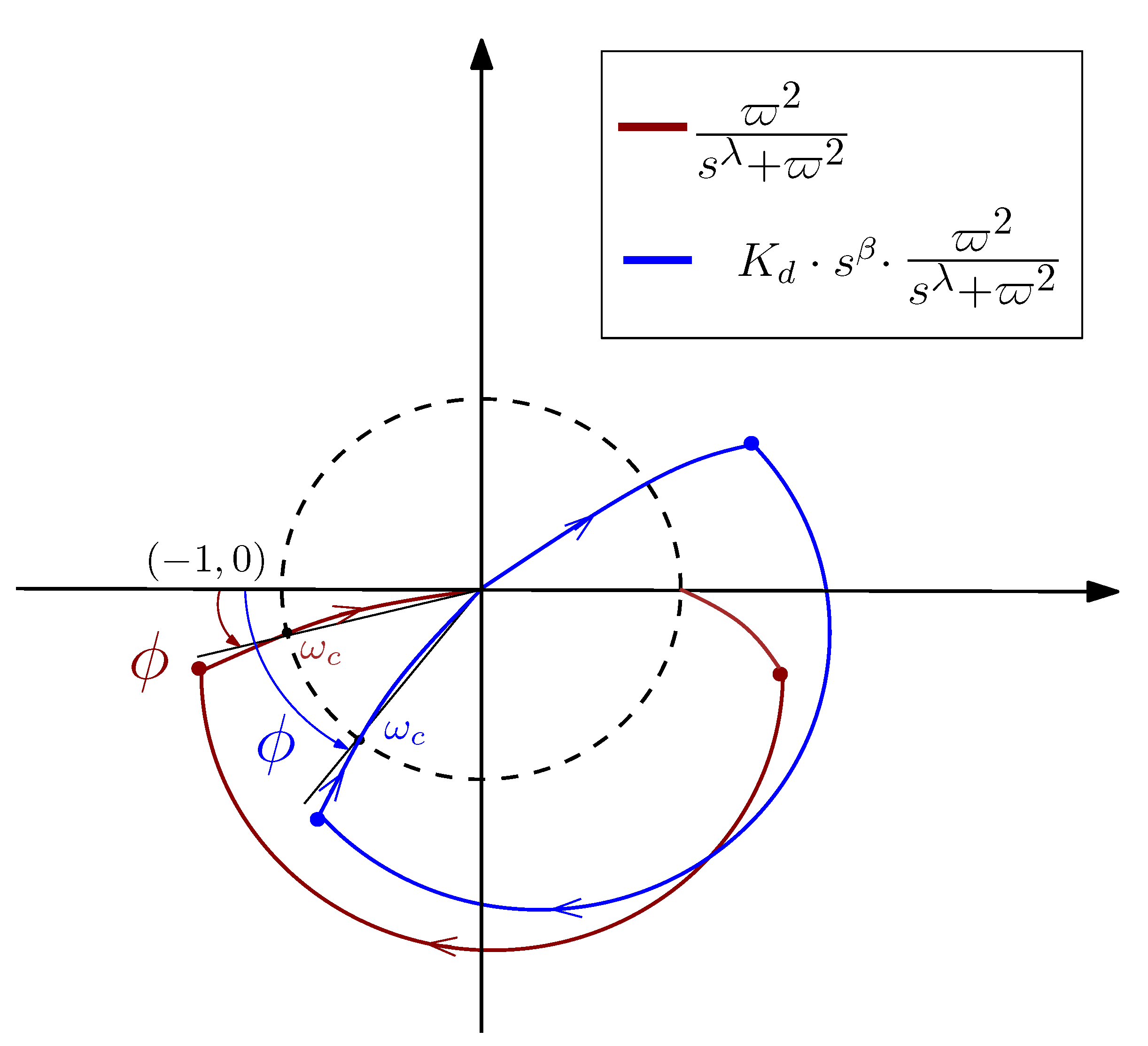
Then, the right side member of (49) is less than or equal to zero and the theorem is proven. □

Remark 1.

In expression (48), both the numerator and denominator are positive, because (41) is verified and the denominator is the same as the one of (49). Then, under the conditions of this theorem, ${\omega }_c$ is increasing with ϖ.

Next, we propose a theorem that facilitates the verification of condition (39).

Theorem 2.

Consider the open-loop transfer function (34) whose gain crossover frequency is represented by ${\omega }_c$. Assume that $1<\lambda \le 2$ and $0<\beta <\lambda$. Moreover, assume a value of the natural frequency of the link ${\varpi }_{-}$ that is greater than one and verifies condition (39). Then, function

$$h\left(\varpi \right)={\varpi }^2+cos\left(\frac{\pi }{2}·\lambda \right)·{\omega }_c^{\lambda }$$

(50)

is less than zero in the interval ${\varpi }_{-}\le \varpi <\infty$.

Proof. 

First, note that ${\omega }_c$ is a function of $\varpi$, according to (43). For this reason, h has a single argument $\varpi$. Differentiating expression (50), we obtain that

$$\frac{dh\left(\varpi \right)}{d\varpi }=2·\varpi +\lambda ·cos\left(\frac{\pi }{2}·\lambda \right)·{\omega }_c^{\lambda -1}·\frac{d{\omega }_c}{d\varpi }$$

(51)

Substituting (48) in (51) and operating yields

$$\begin{array}{c}\frac{dh\left(\varpi \right)}{d\varpi }=\hfill \\ \frac{2}{\varpi }·\frac{\lambda ·{\omega }_c^{\lambda }·\left({\varpi }^2+cos\left(\frac{\pi }{2}·\lambda \right)·{\omega }_c^{\lambda }\right)·\left({\omega }_c^{\lambda }+cos\left(\frac{\pi }{2}·\lambda \right)·{\varpi }^2\right)-\beta ·{\varpi }^2·\left({\omega }_c^{2·\lambda }+2·cos\left(\frac{\pi }{2}·\lambda \right)·{\varpi }^2·{\omega }_c^{\lambda }+{\varpi }^4\right)}{\left(\lambda -\beta \right)·{\omega }_c^{\lambda }·\left({\omega }_c^{\lambda }+cos\left(\frac{\pi }{2}·\lambda \right)·{\varpi }^2\right)-\beta ·{\varpi }^2·\left({\varpi }^2+cos\left(\frac{\pi }{2}·\lambda \right)·{\omega }_c^{\lambda }\right)}\hfill \end{array}$$

(52)

If this expression is particularized at ${\varpi }_{-}$, we have the following:

• Since (39) is verified, inequalities (40) and (41) are also verified. Then, the left addend of the numerator is negative.
• Since inequality (37) is verified, the right addend of the numerator is also negative.
• The denominator is equal to the denominator of (49). Theorem 1 proved that it is positive.

The consequence of these three items is that $\frac{dh\left(\varpi \right)}{d\varpi }<0$ at ${\varpi }_{-}$.

Subsequently, we will prove by contradiction that $h\left(\varpi \right)$ is negative in the interval ${\varpi }_{-}\le \varpi <\infty$. Assume a value ${\varpi }_{+}$ at which $h\left({\varpi }_{+}\right)>0$. Expression (38) shows that ${\omega }_c$ varies continuously with $\varpi$. Then, $h\left(\varpi \right)$ is a continuous function and, consequently, if $h\left({\varpi }_{-}\right)<0$ and $h\left({\varpi }_{+}\right)>0$, a value ${\varpi }_0$ exists such that $h\left({\varpi }_0\right)=0$ and $h\left(\varpi \right)<0$ in the interval $\varpi \in \left[{\varpi }_{-},{\varpi }_0\right)$. The following relation can be established:

$$h\left({\varpi }_0\right)=h\left({\varpi }_{-}\right)+{\int }_{{\varpi }_{-}}^{{\varpi }_0}\left(\frac{dh}{d\varpi }\right)·d\varpi$$

(53)

and, since it has been proved above that $\frac{dh}{d\varpi }<0$ if $h\left(\varpi \right)<0$, the previous integral in the interval $\left[{\varpi }_{-},{\varpi }_0\right]$ is negative. Consequently, $h\left({\varpi }_0\right)<h\left({\varpi }_{-}\right)<0$, which is in contradiction with the previous condition that $h\left({\varpi }_0\right)=0$. □

Assume that $1<\lambda \le 2$ and the payload m varies in the range $\left[\underline{m},\overline{m}\right]$. Then, the natural frequency varies in the range $\left[\underline{\varpi },\overline{\varpi }\right]$ obtained from the previous interval through (5). In the following, we propose a procedure to design controllers robust to payload changes, i.e., to $\varpi$ changes, that verify the specifications of a minimum phase margin ${\underline{\varphi }}_m$ (at $\underline{m}$) and a minimum gain crossover frequency ${\underline{\omega }}_c$ (at $\overline{m}$) in all the range $\left[\underline{m},\overline{m}\right]$:

• Choose the gain crossover frequency ${\underline{\omega }}_c$ corresponding to $\underline{\varpi }$. It must verify condition (39) and, according to Remark 1, it is the minimum ${\omega }_c$ achieved in the interval $\left[\underline{\varpi },\overline{\varpi }\right]$.
• Apply Equation (43) to the pair $\left(\underline{\varpi },\underline{{\omega }_c}\right)$. This gives the relation

  $$k_d=\frac{\chi }{{\underline{\omega }}_c^{\beta }},\chi =\frac{\sqrt{{\underline{\omega }}_c^{2·\lambda }+2·cos\left(\frac{\pi }{2}·\lambda \right)·{\underline{\varpi }}^2·{\underline{\omega }}_c^{\lambda }+{\underline{\varpi }}^4}}{{\underline{\varpi }}^2}$$

  (54)
  Then, to calculate $k_d$, we need to obtain the value of $\beta$, which will be done in the next step.
• In accordance with Theorems 1 and 2, the minimum phase margin in the range $\left[\underline{\varpi },\overline{\varpi }\right]$ is located at $\overline{\varpi }$. This value is represented by ${\underline{\varphi }}_m$. Then, applying condition (42) to $\overline{\varpi }$ and substituting $k_d$ by (54) yields

  $$\chi ·{\left(j·\frac{{\overline{\omega }}_c}{{\underline{\omega }}_c}\right)}^{\beta }·\frac{{\overline{\varpi }}^2}{{(j·{\overline{\omega }}_c)}^{\lambda }+{\overline{\varpi }}^2}=-e^{j·{\underline{\varphi }}_m}$$

  (55)
  This complex equation can be transformed into two real equations that allow us to obtain the two values ${\overline{\omega }}_c$ and $\beta$.
• Obtain $k_d$ from the left side equation of (54) using the already calculated $\chi$ and the fractional order $\beta$ calculated in the previous step.
• Then, the designed controller is

  $$C\left(s\right)=1+k_d·s^{\beta }$$

  (56)

  which can be modified as

  $$C_M\left(s\right)=1+\frac{k_d·s^{\beta }}{{(1+\delta ·s)}^n}$$

  (57)

  where $n=1$ if $\beta <1$ and $n=2$ if $1\le \beta <2$ in order to fulfill the high-frequency noise condition (32). In this expression, $\delta$ is chosen small enough to not modify the frequency characteristic of the open-loop transfer function $L(j·\omega ,\varpi )$. Since this modification produces a phase lag in $L(j·\omega ,\varpi )$, a criterion to design $\delta$ is to choose a value such that the minimum phase margin ${\underline{\varphi }}_m$ is reduced by up to $10\%$ of its initially designed value (or, alternatively, increase ${\underline{\varphi }}_m$ in a quantity that accounts for the phase margin reduction subsequently caused by introducing ${(1+\delta ·s)}^n$).

This algorithm is not iterative: once ${\underline{\varphi }}_m$ and ${\underline{\omega }}_c$ have been defined, the algorithm gives or does not give the solution in a single realization. If the algorithm fails to give a solution, specifications have to be changed. Typically, the problem can be solved by reducing ${\underline{\omega }}_c$.

7. Application to a Single Lumped Mass Flexible Link Manipulator

In this Section, $FO$ controllers are designed for the robotic setup described in Section 2. First, a controller $C_M\left(s\right)$ is designed to apply the procedure described in Section 5 and Section 6 to $UD$-$FOM$ (9), (10). Then, a controller $C_M^{\prime }\left(s\right)$ is designed using $UD$-$IOM$ (4), (6) and the procedure described in Section 5, in such a way that it has the same specifications as $C_M\left(s\right)$ for the nominal payload, in order to make a fair comparison between controllers and assess the effect of using the fractional order model instead of the integer one in the controller design.

7.1. Design of the Controllers

The application of the procedure of Section 6 to design $C_M\left(s\right)$ is as follows:

• The gain crossover frequency corresponding to the minimum natural frequency $\underline{\varpi }=9.42$ rad·s${}^{-1}$ is chosen as ${\underline{\omega }}_c=16$ rad·s${}^{-1}$. Note that the condition $\underline{\varpi }>1$ of Theorem 2 is verified. Then, it is the minimum ${\omega }_c$ achieved in the interval $\left[\underline{\varpi },\overline{\varpi }\right]$.
• Application of the right side equation of (54) gives $\chi =0.81$.
• The minimum phase margin in all the intervals is chosen as $\underline{\varphi }={70}^{\circ }$. Then, the solution of (55) is ${\overline{\omega }}_c=22.33$ rad·s${}^{-1}$ and $\beta =0.65$.
• Obtain $k_d$ from the left side equation of (54) and the fractional order $\beta$ calculated in the previous step. We obtain $k_d=0.148$.
• The proper controller is designed by choosing $\delta =0.16$ and $n=2$ instead of $n=1$ (as stated in the procedure) in order to enhance the filtering of high-frequency noise.

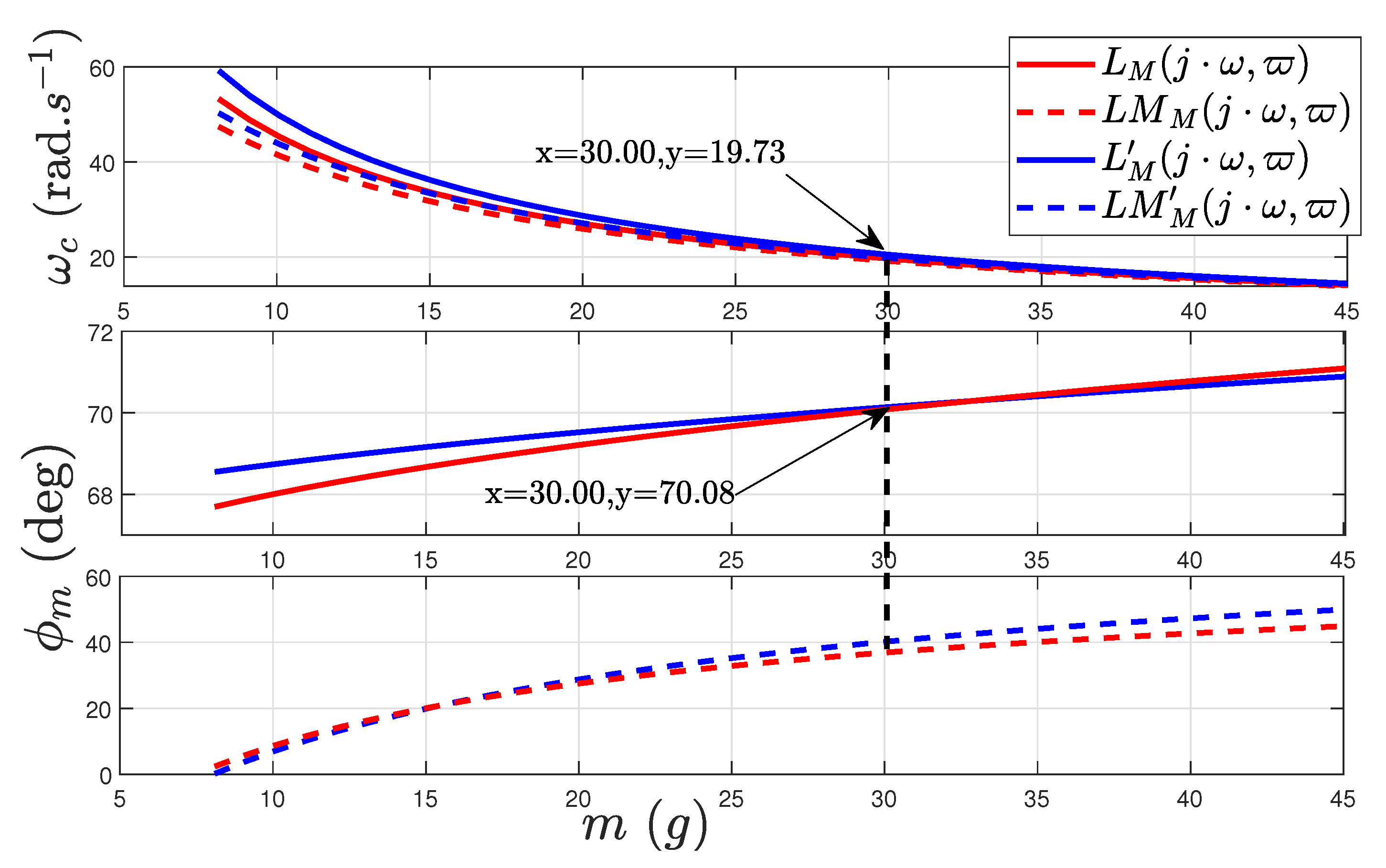
Then, the designed controller is

$$C_M\left(s\right)=1+\frac{0.148·s^{0.65}}{{(1+0.16·s)}^2}$$

(58)

The gain crossover frequency and the phase margin of the $UD$-$FOM$ (9), (10) with controller (58) at the nominal payload $m_{nom}=30$ g are ${\omega }_{c,nom}=19.73$ rad·s${}^{-1}$ and ${\varphi }_{nom}=70.{087}^{\circ }$, respectively.

Subsequently, a control system with the same structure as the previous controller is designed, but assuming the standard undamped integer order model $UD$-$IOM$, i.e, all the parameters of the control system are tuned to this model making $\lambda =2$ in all the expressions of Section 5. In order to make a fair comparison with the previous design, this controller is tuned to have the same frequency specifications ${\omega }_{c,nom}$ and ${\varphi }_{nom}$ as the previous controller at the nominal payload.

Imposing the complex condition (42) and making $\lambda =2$, $\varphi ={\varphi }_{nom}$ and ${\omega }_c={\omega }_{c,nom}$ in this equation, we obtain $k_d=0.241$ and $\beta =0.65$. Then, the controller designed using the integer order model is

$$C_M^{\prime }\left(s\right)=1+\frac{0.241·s^{0.65}}{{(1+0.16·s)}^2}$$

(59)

Figure 10 illustrates the variations of the gain crossover frequency ${\omega }_c$ and the margin phase ${\varphi }_m$ of the open-loop transfer function in function of the payload, when using the two controllers $C_M$ and $C_M^{\prime }$ and including or not including the inner loop motor dynamics, i.e., in the cases:

$$\begin{array}{c}{L}_M(j·\omega ,\varpi )={\widehat{C}}_M(j·\omega )·G^{1.92}(j·\omega ,\varpi )\hfill \\ L_M^{\prime }(j·\omega ,\varpi )={\widehat{C}}_M^{\prime }(j·\omega )·G^{1.92}(j·\omega ,\varpi )\hfill \\ L{M}_M(j·\omega ,\varpi )={\widehat{C}}_M(j·\omega )·G^{1.92}(j·\omega ,\varpi )·M(j·\omega )\hfill \\ L{M}_M^{\prime }(j·\omega ,\varpi )={\widehat{C}}_M^{\prime }(j·\omega )·G^{1.92}(j·\omega ,\varpi )·M(j·\omega )\hfill \end{array}$$

(60)

In these expressions, $M\left(s\right)$ has its poles in $z=-80$ (see expression (21)). We notice in this figure that

• The plots of ${\omega }_c$ and ${\varphi }_m$ intersect at the nominal payload in the cases of $L_M(j·\omega ,\varpi )$ and $L_M^{\prime }(j·\omega ,\varpi )$.
• ${\omega }_c$ is decreasing with m (increasing with $\varpi$) as stated in Remark 1.
• ${\varphi }_m$ is increasing with m (decreasing with $\varpi$) as stated in Theorem 1.

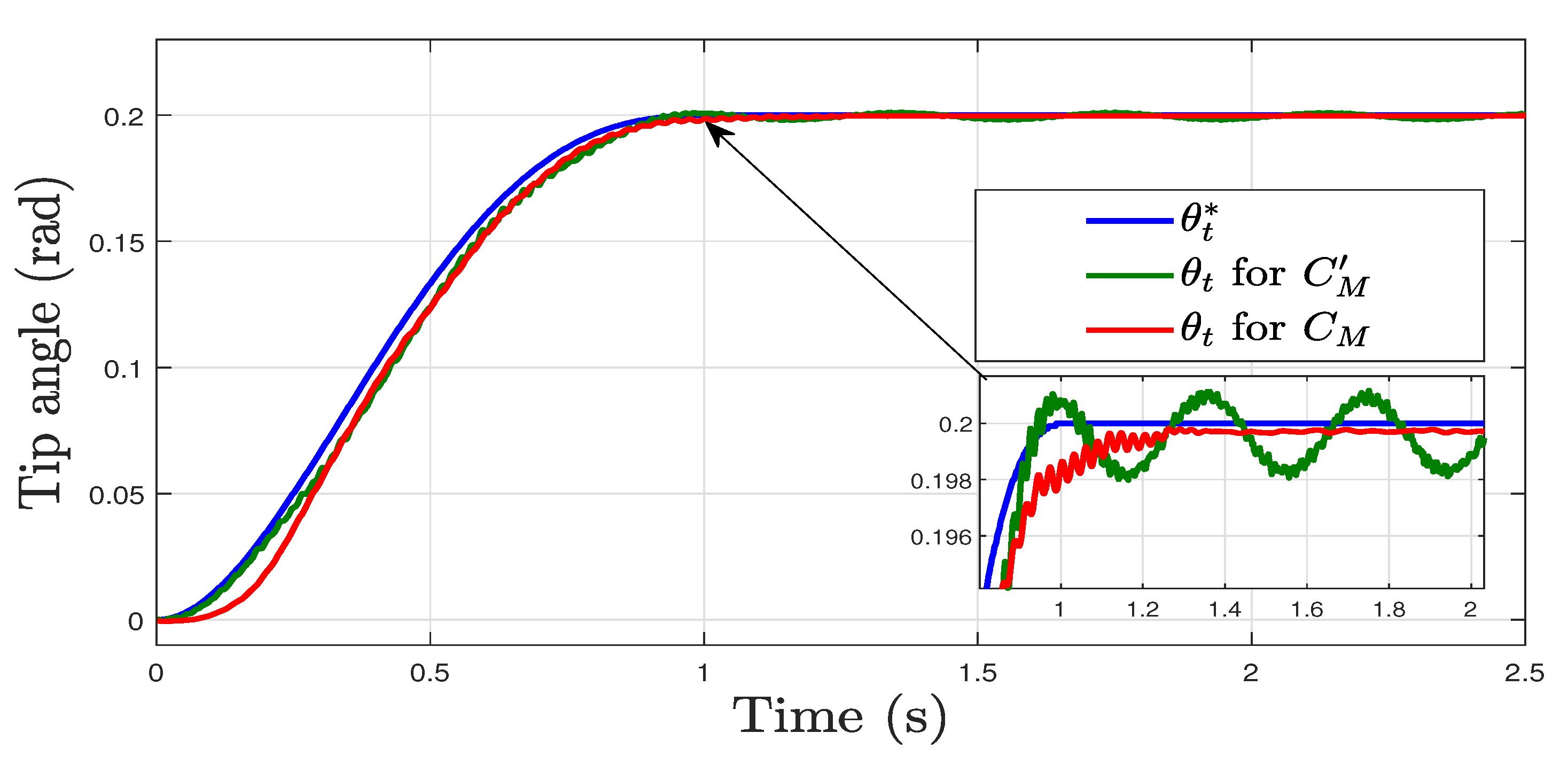
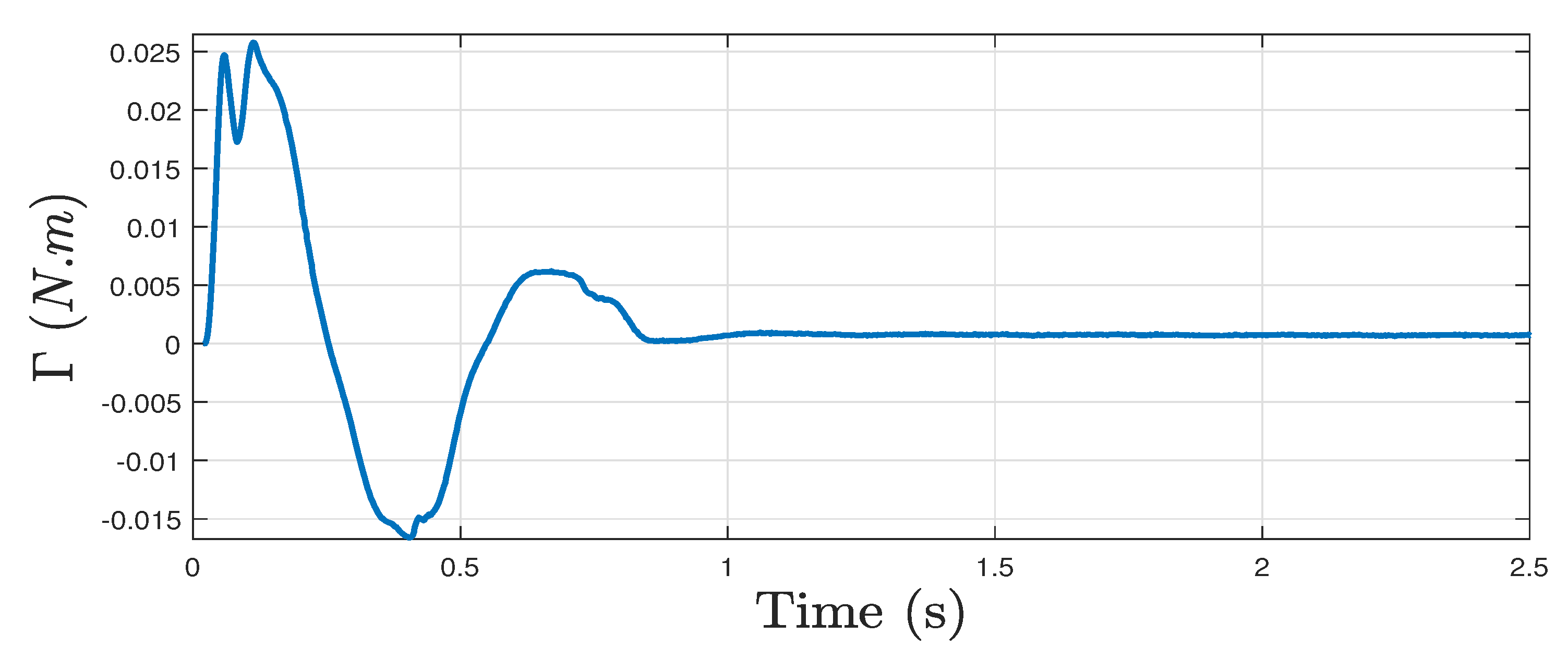
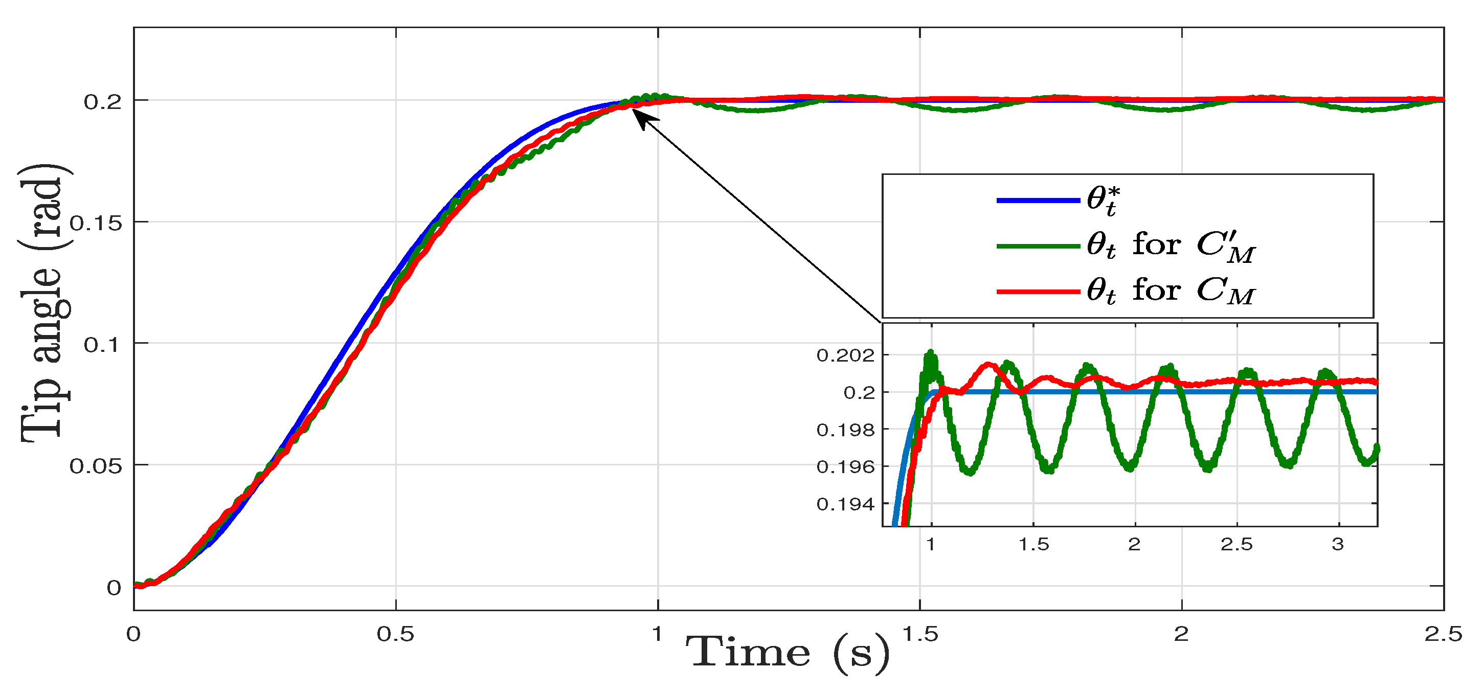
7.2. Experimental Validation of the Controller

Figure 11, Figure 12 and Figure 13 show the experimental trajectory tracking of the robot achieved using controllers $C_M\left(s\right)$ (58) and $C_M^{\prime }\left(s\right)$ (59), in the cases of the nominal (m = 30 g) payload, and the maximum (m = 40 g) and the minimum (m = 20 g) payloads that have been used in the design of the robust controller. These experiments were carried out using strain gauges that have a small offset, as Figure 14 shows in the steady state of an example of trajectory tracking. These results show that (1) both $C_M\left(s\right)$ and $C_M^{\prime }\left(s\right)$ controllers remove the steady-state error in the tip position caused by the strain gauge offset; (2) the responses using $C_M^{\prime }\left(s\right)$ are slightly more oscillatory than when using $C_M\left(s\right)$, especially in the case of the minimum payload; and (3) the robot’s responses when tracking a trajectory in the cases of the nominal and the maximum payload are approximately the same using both controllers. To sum up, both controllers provide good trajectory tracking in the cases of the nominal and minimum resonant frequencies with steady-state error elimination and zero overshoot. In the case of the maximum resonant frequency—associated with the minimum mass m = 20 g—the tip oscillations are completely damped using the $C_M\left(s\right)$ controller, while small oscillations remain if $C_M^{\prime }\left(s\right)$ is used.

Finally, we show that the closed-loop behavior is appropriate in the most challenging case of carrying very low payloads that are outside the payload interval used for the design of controller (58). Figure 15 and Figure 16 show the responses of both controllers for m = 16 g and m = 8 g. Large oscillations can be seen in both figures in the responses obtained using $C_M^{\prime }\left(s\right)$, while controller $C_M\left(s\right)$ still damps the oscillations in the case of m = 16 g and yields an oscillation of much lower amplitude than the one of $C_M^{\prime }\left(s\right)$ in the case of m = 8 g.

7.3. Discussion

At first sight, one might think that using a fractional model of order $1.92$ instead of the well-known integer model of order 2 in the design of the control system of our $FLR$ would be irrelevant since these are very close orders. However, our analysis and experimental results show that it makes a significant difference in the closed-loop dynamics when low payloads have to be translated. Next, we analyze the reason for these differences.

We observe in Figure 10 that:

• At payloads lower than the nominal payload, the gain crossover frequency of $L_M^{\prime }$ is higher than that of $L_M$ and the gain crossover frequency of $L{M}_M^{\prime }$ is higher than that of $L_M^{\prime }$.
• At payloads lower than the nominal payload, the gain crossover frequency of $L{M}_M$ is lower than that of $L_M$ and the gain crossover frequency of $L{M}_M^{\prime }$ is lower than that of $L_M^{\prime }$. This can be easily understood because $M\left(s\right)$ is a low-pass filter that reduces the amplitudes of $L_M$ and $L_M^{\prime }$, causing a reduction in the gain crossover frequencies.
• The effect of adding $M\left(s\right)$ to the open loop is a strong reduction in the phase margin at all the payloads, as a comparison of the middle and lower subplots shows.
• At payloads lower than the nominal payload, the phase margin of $L_M^{\prime }$ is higher than that of $L_M$.
• However, the lower subplot of Figure 10 shows that, at low payloads, the phase margin of $L{M}_M$ is higher than that of $L{M}_M^{\prime }$. This is caused by the fact that, according to the higher subplot of Figure 10, the gain crossover frequency of $L{M}_M$ is lower than that of $L{M}_M^{\prime }$. Then, $M\left(s\right)$ produces less phase lag on $L_M$ than on $L_M^{\prime }$. This compensates for the positive difference in the phase margin between $L_M^{\prime }$ and $L_M$, yielding higher phase margins of $L{M}_M$ at low payloads.

This last issue has been corroborated via the experiments carried out with small and very small payloads.

8. Conclusions

The robust control of very lightweight flexible link robots has been addressed in this paper. In these robots, it is often assumed that all the mass is lumped in the tip payload. Then, their dynamics have a single vibration mode with little damping. A control strategy for this robot needs to guarantee robustness to (1) the nonlinear motor frictions, (2) the offset and the high-frequency noises of the strain gauge sensor implemented in the robot platform and (3) the variations of the carried payload. We achieved these objectives in previous work [31].

Usually, robot damping is modeled by adding to the Euler–Bernoulli beam equation a term proportional to the angular velocity of the robot (see (15)). However, we have proven experimentally that, for our specific robot, a better fitting of the damping phenomenon is achieved modifying Newton’s second law of motion by using an $FO$ derivative of the angle instead of the standard second order derivative (see (10)). Then, the input-state feedback linearization method based on the singular perturbation technique and an $FO$$PD$ controller—which was used in [31]—was modified to account for such a fractional order model.

The contributions of this paper are therefore as follows: (1) experimental justification of the fact that, in some cases, the damping phenomena of the dynamics of flexible link robots are better fitted using models based on the generalization of Newton’s second law of motion by using FO differentiation; (2) a new fractional input-state feedback linearization scheme; (3) a lemma and two theorems that allowed us to define a procedure to tune the $FO$ controller embedded in this control scheme; and (4) proving analytically and experimentally the advantage of this new control system based on the $FOM$ over the previous control based on the input-state feedback linearization method that, though yielding an $FO$$PD$ controller, its design was based on the standard integer order model. These advantages are noticeable at low and very low payloads, cases in which the natural vibration frequency of the robot becomes very high and the closed-loop control is prone to instability.

Our future work will be focused on extending this $FOM$ and controller to multilink robots.

References

1. Spong, M.W.; Hutchinson, S.; Vidyasagar, M. Robot Modeling and Control; John Wiley & Sons: Hoboken, NJ, USA, 2020. [Google Scholar]
2. Monje, C.; Ramos, F.; Feliu, V.; Vinagre, B. Tip position control of a lightweight flexible manipulator using a fractional order controller. IET Control Theory Appl. 2007, 1, 1451–1460. [Google Scholar] [CrossRef]
3. Rahimi, H.; Nazemizadeh, M. Dynamic analysis and intelligent control techniques for flexible manipulators: A review. Adv. Robot. 2014, 28, 63–76. [Google Scholar] [CrossRef]
4. Subedi, D.; Tyapin, I.; Hovland, G. Review on modeling and control of flexible link manipulators. Model. Identif. Control 2020, 41, 141–163. [Google Scholar] [CrossRef]
5. Feliu-Batlle, V.; Rattan, K.; Brown, H. Modelling and Control of Single-Link Flexible Arms with Lumped Masses. ASME J. Dyn. Syst. Meas. Control 1992, 114, 59–69. [Google Scholar] [CrossRef]
6. Cambera, J.C.; Feliu-Batlle, V. Input-state feedback linearization control of a single-link flexible robot arm moving under gravity and joint friction. Robot. Auton. Syst. 2017, 88, 24–36. [Google Scholar] [CrossRef]
7. Wei, J.; Cao, D.; Liu, L.; Huang, W. Global mode method for dynamic modeling of a flexible-link flexible-joint manipulator with tip mass. Appl. Math. Model. 2017, 48, 787–805. [Google Scholar] [CrossRef]
8. Gao, H.; He, W.; Zhou, C.; Sun, C. Neural network control of a two-link flexible robotic manipulator using assumed mode method. IEEE Trans. Ind. Inform. 2018, 15, 755–765. [Google Scholar] [CrossRef]
9. Farid, M.; Cleghorn, W.L. Dynamic modeling of multi-flexible-link planar manipulators using curvature–based finite element method. J. Vib. Control 2014, 20, 1682–1696. [Google Scholar] [CrossRef]
10. Zhang, X.; Sørensen, R.; Iversen, M.R.; Li, H. Computationally efficient dynamic modeling of robot manipulators with multiple flexible-links using acceleration-based discrete time transfer matrix method. Robot. Comput.-Integr. Manuf. 2018, 49, 181–193. [Google Scholar] [CrossRef]
11. Kiang, C.T.; Spowage, A.; Yoong, C.K. Review of control and sensor system of flexible manipulator. J. Intell. Robot. Syst. 2015, 77, 187–213. [Google Scholar] [CrossRef]
12. Singh, A.P.; Deb, D.; Agarwal, H. On selection of improved fractional model and control of different systems with experimental validation. Commun. Nonlinear Sci. Numer. Simul. 2019, 79, 104902. [Google Scholar] [CrossRef]
13. Singh, A.P.; Deb, D.; Agrawal, H.; Bingi, K.; Ozana, S. Modeling and control of robotic manipulators: A fractional calculus point of view. Arab. J. Sci. Eng. 2021, 46, 9541–9552. [Google Scholar] [CrossRef]
14. Li, M. Theory of Fractional Engineering Vibrations; De Gruyter: Berlin, Germany, 2021. [Google Scholar]
15. Wang, P.; Wang, Q.; Xu, X.; Chen, N. Fractional Critical Damping Theory and Its Application in Active Suspension Control. Shock Vib. 2017, 2017, 2738976. [Google Scholar] [CrossRef]
16. Mattioni, A.; Wu, Y.; Le Gorrec, Y. Infinite dimensional model of a double flexible-link manipulator: The Port-Hamiltonian approach. Appl. Math. Model. 2020, 83, 59–75. [Google Scholar] [CrossRef]
17. Baek, J.; Jin, M.; Han, S. A new adaptive sliding-mode control scheme for application to robot manipulators. IEEE Trans. Ind. Electron. 2016, 63, 3628–3637. [Google Scholar] [CrossRef]
18. Becedas, J.; Trapero, J.R.; Feliu, V.; Sira-Ramírez, H. Adaptive controller for single-link flexible manipulators based on algebraic identification and generalized Proportional Integral control. IEEE Trans. Syst. Man Cybern. Part B (Cybern.) 2009, 39, 735–751. [Google Scholar] [CrossRef]
19. Alandoli, E.A.; Lee, T.S.; Lin, Y.; Vijayakumar, V. Dynamic model and intelligent optimal controller of flexible link manipulator system with payload uncertainty. Arab. J. Sci. Eng. 2021, 46, 7423–7433. [Google Scholar] [CrossRef]
20. Ouyang, Y.; He, W.; Li, X.; Liu, J.K.; Li, G. Vibration Control Based on Reinforcement Learning for a Single-link Flexible Robotic Manipulator. IFAC-PapersOnLine 2017, 50, 3476–3481. [Google Scholar] [CrossRef]
21. Mamani, G.; Becedas, J.; Feliu, V. Sliding Mode Tracking Control of a Very Lightweight Single-Link Flexible Robot Robust to Payload Changes and Motor Friction. J. Vib. Control 2012, 18, 1141–1155. [Google Scholar] [CrossRef]
22. Karimi, H.; Yazdanpanah, M.J.; Patel, R.; Khorasani, K. Modeling and control of linear two-time scale systems: Applied to single-link flexible manipulator. J. Intell. Robot. Syst. 2006, 45, 235–265. [Google Scholar] [CrossRef]
23. Nikdel, N.; Badamchizadeh, M.; Azimirad, V.; Nazari, M.A. Fractional-order adaptive backstepping control of robotic manipulators in the presence of model uncertainties and external disturbances. IEEE Trans. Ind. Electron. 2016, 63, 6249–6256. [Google Scholar] [CrossRef]
24. Gupta, S.; Singh, A.P.; Deb, D.; Ozana, S. Kalman Filter and Variants for Estimation in 2DOF Serial Flexible Link and Joint Using Fractional Order PID Controller. Appl. Sci. 2021, 11, 6693. [Google Scholar] [CrossRef]
25. Dumlu, A.; Erenturk, K. Trajectory tracking control for a 3-dof parallel manipulator using fractional-order PIλDμ control. IEEE Trans. Ind. Electron. 2013, 61, 3417–3426. [Google Scholar] [CrossRef]
26. Relaño, C.; Muñoz, J.; Monje, C.A.; Martínez, S.; González, D. Modeling and Control of a Soft Robotic Arm Based on a Fractional Order Control Approach. Fractal Fract. 2022, 7, 8. [Google Scholar] [CrossRef]
27. Sabouri, J.; Effati, S.; Pakdaman, M. A neural network approach for solving a class of fractional optimal control problems. Neural Process. Lett. 2017, 45, 59–74. [Google Scholar] [CrossRef]
28. Lopes, A.M.; Tenreiro Machado, J.A. Fractional-order sensing and control: Embedding the nonlinear dynamics of robot manipulators into the multidimensional scaling method. Sensors 2021, 21, 7736. [Google Scholar] [CrossRef]
29. Mujumdar, A.; Tamhane, B.; Kurode, S. Fractional order modeling and control of a flexible manipulator using sliding modes. In Proceedings of the 2014 American Control Conference, Portland, OR, USA, 4–6 June 2014; pp. 2011–2016. [Google Scholar]
30. Bingi, K.; Rajanarayan Prusty, B.; Pal Singh, A. A Review on Fractional-Order Modelling and Control of Robotic Manipulators. Fractal Fract. 2023, 7, 77. [Google Scholar] [CrossRef]
31. Gharab, S.; Benftima, S.; Batlle, V.F. Fractional Control of a Lightweight Single Link Flexible Robot Robust to Strain Gauge Sensor Disturbances and Payload Changes. Actuators 2021, 10, 317. [Google Scholar] [CrossRef]
32. Feliu-Talegon, D.; Feliu-Batlle, V.; Castillo-Berrio, C. Motion control of a sensing antenna with a nonlinear input shaping technique. Rev. Iberoam. Autom. Inform. Ind. 2016, 13, 162–173. [Google Scholar] [CrossRef] [Green Version]
33. Feliu, V.; Pereira, E.; Díaz, I.M. Passivity-based control of single-link flexible manipulators using a linear strain feedback. Mech. Mach. Theory 2014, 71, 191–208. [Google Scholar] [CrossRef]
34. Herrmann, R. Fractional Calculus: An Introduction for Physicists; World Scientific: Singapore, 2011. [Google Scholar]
35. Chung, W.S. Fractional Newton mechanics with conformable fractional derivative. J. Comput. Appl. Math. 2015, 290, 150–158. [Google Scholar] [CrossRef]
36. Feliu-Talegon, D.; Feliu-Batlle, V. Control of very lightweight 2-DOF single-link flexible robots robust to strain gauge sensor disturbances: A fractional-order approach. IEEE Trans. Control Syst. Technol. 2021, 30, 14–29. [Google Scholar] [CrossRef]
37. Kashiri, N.; Malzahn, J.; Tsagarakis, N.G. On the sensor design of torque controlled actuators: A comparison study of strain gauge and encoder-based principles. IEEE Robot. Autom. Lett. 2017, 2, 1186–1194. [Google Scholar] [CrossRef]
38. Benftima, S.; Batlle, V.F.; Benattia, S.; Salhi, S. A Fast Online Estimator of the Main Vibration Mode of Mechanisms from a Biased Slightly Damped Signal. In Proceedings of the IECON 2022—48th Annual Conference of the IEEE Industrial Electronics Society, Brussels, Belgium, 17–20 October 2022; pp. 1–6. [Google Scholar]
39. Fliess, M. Analyse non standard du bruit. C. R. Acad. Sci. Paris Ser. I 2006, 342, 797–802. [Google Scholar] [CrossRef] [Green Version]
40. Ogata, K. Modern Control Engineering; Prentice Hall: Hoboken, NJ, USA, 1993. [Google Scholar]
41. Feliu-Batlle, V. Robust isophase margin control of oscillatory systems with large uncertainties in their parameters: A fractional-order control approach. Int. J. Robust Nonlinear Control 2017, 27, 2145–2164. [Google Scholar] [CrossRef]
Figure 1. Air Table Flexible Robot System.
Fractalfract 07 00504 g001
Figure 2. Schematic Representation of a Single Link Flexible manipulator.
Fractalfract 07 00504 g002
Figure 3. Comparison of the Different Predicted Torque Models.
Fractalfract 07 00504 g003
Figure 4. Comparison of the Different Predicted Torques for the Nominal Payload.
Fractalfract 07 00504 g004
Figure 5. Comparison of the Different Predicted Torques for the Maximum Payload.
Fractalfract 07 00504 g005
Figure 6. Comparison of the Different Predicted Torques for the Minimum Payload.
Fractalfract 07 00504 g006
Figure 7. Inner Control Loop Scheme.
Fractalfract 07 00504 g007
Figure 8. Outer Control Loop Scheme.
Fractalfract 07 00504 g008
Figure 9. Nyquist Plots.
Fractalfract 07 00504 g009
Figure 10. Open-loop Frequency Characteristics using Controllers (58) and (59).
Fractalfract 07 00504 g010
Figure 11. Trajectory Tracking using Controllers (58) and (59) with the Nominal Payload (30 g).
Fractalfract 07 00504 g011
Figure 12. Trajectory Tracking using Controllers (58) and (59) with the Maximum Payload (40 g).
Fractalfract 07 00504 g012
Figure 13. Trajectory Tracking using Controllers (58) and (59) with the Minimum Payload (20 g).
Fractalfract 07 00504 g013
Figure 14. Strain Gauge Measurement of the Torque at the Base of the Link when the Robot Performs a Trajectory.
Fractalfract 07 00504 g014
Figure 15. Trajectory Tracking using Controllers (58) and (59) with a Small Payload out of the Robustness Design Interval (16 g).
Fractalfract 07 00504 g015
Figure 16. Trajectory Tracking using Controllers (58) and (59) with a Very Small Payload out of the Robustness Design Interval (8 g).
Fractalfract 07 00504 g016