Abstract
Xylella fastidiosa is a phytobacterium able to provoke severe diseases in many species. When it infects olive trees, it induces the olive quick decline syndrome that leads the tree to a rapid desiccation and then to the death. This phytobacterium has been recently detected in olive groves in southern Italy, representing an important threat to the olive growing of the area. In this paper, in order to identify patterns revealing the presence of Xylella fastidiosa, several hundreds pixels of MODIS satellite evapostranspiration covering infected and healthy olive groves in southern Italy were analyzed by means of the Fisher–Shannon method and the multifractal detrended fluctuation analysis. The analysis of the receiver operating characteric curve indicates that the two informational quantities (the Fisher information measure and the Shannon entropy) and the three multifractal parameters (the range of generalized Hurst exponents and the width and the maximum of the multifractal spectrum) are well suited to discriminate between infected and healthy sites, although the maximum of the multifractal spectrum performs better than the others. These results could suggest the use of both the methods as an operational tool for early detection of plant diseases.
1. Introduction
The climate change is rapidly evolving in time and the world connections are more and more increasing; these two factors represent an important driver of biological invasions [1,2], which have favored the establishment of extremely dangerous phytopathogens such as Xylella fastidiosa [3]. This bacterium is transmitted by several vectors, such as the Homalodisca vitripennis, a sap-sucking leafhopper, native to southeastern United States and northeastern Mexico [4]. Xylella fastidiosa affects plants, inducing several infections, such as the Pierce’s disease of grapevines [5], the olive quick decline [6], the bacterial leaf scorch [7], and the phony peach disease [8], causing significant important economic loss in agriculture. In Europe, Xylella fastidiosa was detected for the first time in southeastern Italy in 2013 [9], and then it spread out to several other European countries, representing a real phyto-sanitary emergency [10]. The first study focused on Xylella fastidiosa was performed by Krugner et al. [11], who detected Xylella fastidiosa subsp. multiplex in olive trees affected by leaf scorch and branch dieback; however, in their laboratory experiments they did not see the same symptoms in olive trees as those found in the field. After Xylella fastidiosa was detected in olive groves in southeastern Italy, a systematic study on Xylella fastidiosa was carried out in Argentina and Brazil, where symptomatic olive trees were found to host Xylella fastidiosa subsp. pauca [12,13], which was the same subspecies found in the Italian olive trees [14]. Strona et al. [15] found that the wide distribution of olive groves in Apulia (southeastern Italy) and the large amount of Philaenus spumarius L., vector of this bacterium, could have favored the embedding of Xylella fastidiosa in this territory.
Since no treatment has yet been found to allow the infected trees to recover, and effective strategy to impede the epidemy to spread out is just plucking the infected trees, it is clear that to lower the risk of spreading the infection relies on an early identification of asymptomatic or infected trees with visible symptoms of desiccation. The visual inspection still represents the most commonly adopted approach, which is rapid, easy, and cost-effective; however, the accuracy of identification depends on the the subjective assessment of the level of the disease. Moreover, since the collected samples can only be analyzed in the laboratory, the visual inspection becomes a time-consuming, expensive, and destructive method of detection of Xylella fastidiosa [16].
Recently, remote sensing (RS) has become a useful technology aiming at monitoring the vegetation status, and also its relationship with the detection of plant diseases and infections. For instance, the use of unmanned aerial vehicle (UAVs) in combination with a multispectral radiometer to classify the severity of plant infection [17], or the airborne imaging spectroscopy combined with thermography to reveal pre-symptomatic infection patterns [18], or the use of an RS-driven support vector machine model to predict accurate plant disease spatial distribution [19], represent a few examples of application of RS employed in the detection of Xylella fastidiosa.
In this paper, we analyze the time dynamics of MODIS satellite evapotranspiration (ET) data (free available in the Google Earth Engine cloud database) of a large part of southern Italy covered by olive groves, some infected by Xylella fastidiosa. Since the infection mechanism of Xylella fastidiosa is given by the obstruction of the vessels that carry water and nutrients from the roots to the stem and up to the leaves, the infected plants dry up completely; thus, the use of ET data, which are related to the water content of the plants, seems suitable to assess the presence of plant diseases due to Xylella fastidiosa.
For our investigation purposes, we will use the Fisher–Shannon analysis [20,21] and the multifractal detrended fluctuation analysis (MFDFA) [22], which are well-known statistical methods capable of characterizing the complexity of time series in terms of informational and multiscaling behavior, such as that of ET, which would reflect the transformation processes of the trees.
2. Methods
2.1. The Periodogram Analysis and Spectral Filtering
Given a time series , for , where N is the length of the series, its discrete Fourier transform (DFT) is defined as
where i is the imaginary unit and
The series can be obtained from its DFT by
The periodogram of is defined as
A peak in the periodogram at a frequency indicates a periodicity in the time series with period . The removal of this periodicity from the time series (spectral filtering) is performed by removing and from Equation (4).
2.2. The Fisher–Shannon Analysis
The Fisher–Shannon analysis is based on the calculation of two informational quantities: the Fisher information measure (FIM) and Shannon entropy (SE), which locally and globally, respectively, quantify the type of smoothness of the probability distribution function of the time series, with the FIM being an indicator of the order and organization [20], and the SE an indicator of the uncertainty or disorder of the series [21]. Their definitions are as follows:
where f(x) is the distribution of the series’ values x. The Shannon entropy power NX, which is always positive, is generally used instead of SE:
FIM and NX are linked by the isoperimetric inequality [23], where D is the dimension of the space (1 for time series). The so-called Fisher–Shannon information plane (FSIP), whose coordinate axes are FIM and NX, can be used to represent time series with points that can occupy only the domain , where the minimum is only for series with a Gaussian distribution. Thus, the FSIP, combining the global and local properties of SEP and FIM, respectively, could furnish a useful means of discrimination between different time dynamics of time series [23].
2.3. The Multifractal Detrended Fluctuation Analysis
The multifractal detrended fluctuation analysis (MFDFA) [22] is a well-known multifractal method, efficiently used to investigate the multifractality of time series, characterized by heterogeneity, intermittency, and different roles played by small and large fluctuations. Considering the series , for with mean , its profile is obtained by a simple integration:
The profile is divided into contiguous boxes of identical size m that are called scale. In case N is not a multiple of m, since a short part of the series could remain at the end, the same procedure is applied from the end of the profile . In each of the boxes, the profile is fitted with a p-degree polynomial by a least square method, obtaining the following variance:
and
where is the p-degree polynomial fitting the profile in the box ; the polynomial, thus, removes all the trends until the order p in the profile, and until the order p-1 in the original time series. Then, the qth order fluctuation function is calculated as
where . For , is calculated as follows:
from which the exponent is obtained. For the large fluctuations are enhanced, while for the small ones are highlighted. The fluctuation function increases with the box size or scale m; but if such increase is a power law, then the series is characterized by long-range power law correlations:
where is called generalized Hurst exponent. If the exponent is nearly constant with q, the series is called monofractal, indicating that the scaling behavior of the small and large fluctuations is approximately identical. If the small and large fluctuations have different scaling behaviors, decreases with q, indicating that more exponents are necessary to describe the fractality of the series that, in this case, is multifractal with a more complex structure. The range of the exponents (-range) is employed to quantify the multifractality of a series. The larger the -range, the larger the multifractal degree of the series. The degree of multifractality can be investigated by means of the multifractal spectrum. From the following relationships (also known as the Legendre transform),
and
the multifractal spectrum is calculated as
where is the so-called Hölder exponent. The multifractal spectrum furnishes an indication of the relative dominance of the various scaling exponents in the series and is typically single-humped shaped. It can be fitted by a second-degree polynomial:
where is the maximum. The width W of the multifractal spectrum is defined as
where and are the two zeros of the fitted second-degree polynomial. W is often employed to quantify the multifractality in a series. The larger the value of W, the higher the multifractal degree of the series. The maximum of the multifractal spectrum conveys information about the regular behavior of the process, and it is high for less-regular processes with a finer structure, and small for more regular ones.
2.4. The ROC Analysis
The receiver operating characteristics (ROC) analysis is used for selecting classifiers based on their performance. In binary classification problems, an instance can be labeled as positive or negative, and a classifier maps instance to predicted classes.
Given a classifier and an instance, there are four possible outcomes. The instance is counted (1) as a true positive (TP) if it positive and it is classified as positive; (2) as a false negative (FN) if it is positive and classified as negative; (3) as a true negative (TN) if is negative and is classified as negative; and (4) as a false positive (FP) if it is negative and classified as positive [24]. We can define the following ratios, the true positive rate (TPr) and the false positive rate (FPr):
The sensitivity is the TPr and the specificity is 1-FPr. An ROC curve is a two-dimensional graph in which the sensitivity is plotted on the Y axis and 1-specificity is plotted on the X axis. In the ROC space, the point (0,1) represents perfect classification, and one point is better than another if it is to the northwest of the first. The diagonal line represents the random classification, and a good classifier has to be represented by a point located in the upper triangle of the ROC space.
Some classifiers yield a score, a numeric value that represents the degree to which an instance is a member of a class. Such a scoring classifier can be used with a threshold to produce a binary classifier, and depending upon the relationship between the output and the threshold, the classifier produces a positive or a negative. Each threshold value produces a point in ROC space; varying the threshold from two extremal values, a curve can be traced through ROC space; this curve is called the ROC curve. The area under the ROC curve (AUC) is generally used to quantify the performance of the classifier. Each point on the ROC curve represents a sensitivity/specificity tradeoff corresponding to a particular threshold. Generally, to maximize such a tradeoff, the point of the ROC curve closest to (0,1) is considered and the corresponding threshold is used.
3. Data and Study Area
Since the effect of the infection by Xylella fastidiosa in olive trees is the rapid branch desiccation [25], we analyzed the Moderate Resolution Imaging Spectroradiometer (MODIS) evapotranspiration (ET) data that are able to monitor the water status of plants and, thus, to detect signs of the presence of disease. The data, which have 500 m spatial resolution and are eight-day sampled, are freely available online (https://lpdaac.usgs.gov) and in the Google Earth Engine (GEE) cloud database. The ET is calculated, summing up soil evaporation (), canopy evaporation (), and canopy transpiration ():
with
where is the canopy cover, is the pixel wet surface fraction, RH is the relative humidity, is the gradient of the saturation vapor pressure–temperature, and are the available energy to the soil and canopy, respectively, is the psychrometric constant, is a parameter related to the soil moisture constraint, and are the surface and aerodynamic resistance for the soil surface, and are the surface and aerodynamic resistance for the wet canopy evaporation, and and are the surface and aerodynamic resistance for the canopy transpiration [26].
The analyzed ET data cover the southeastern part of Italy (Figure 1) from 2010 through the present. The length of each pixel time series is 575, and data missing percentage is less than 25%. We investigated areas infected and not infected by Xylella fastidiosa. For the infected area, the number of analyzed pixels is 996, while that of the not-infected area is 1023.
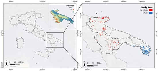
Figure 1.
Infected and healthy sites. The infected sites were selected on the basis of [27].
The areas occupied by infected and uninfected plants are in different locations, neither overlapping nor neighboring. The selection of both types of areas (infected and uninfected) was driven by the fact that they are quite homogeneous from the topographical (as shown in the inset of Figure 1) and climatic points of view. These areas are quite flat, especially in the SE part of Apulia (where infected olive trees have been detected) and in the NE part of Apulia and along the Ionian coast of Basilicata (where no traces of Xylella fastidiosa have been found so far), with hilly topographic features in the NE part of Basilicata, characterized by a distinctly Mediterranean climate with cold winters and hot and dry long summers.
4. Results
The ET time series are characterized by oscillating variability, as shown by Figure 2, which represents, as an example, the time variation of ET of a pixel of infected area. Figure 3 and Figure 4 show the periodogram and the heat map of the pixel time series of the infected and not-infected areas; all pixels are modulated by annual and sub-annual (6, 4, and 3 months) cycles that represent the phenological cycles of vegetation correlated with the meteo-climatic oscillations. In order to investigate the inner time dynamics of vegetation not driven by the meteo-climatic oscillations, we filtered them out and analyzed the residuals. Figure 5 shows the normalized residual after the spectral filtering of the pixel time series shown in Figure 2.
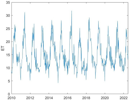
Figure 2.
Pixel time series of an infected site.
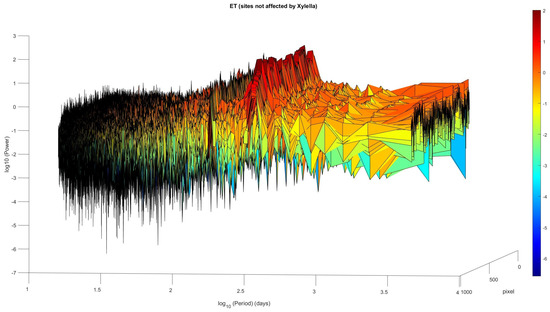
Figure 3.
Periodogram of the time series of the MODIS ET pixels covering the not-infected area.
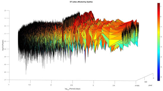
Figure 4.
Periodogram of the time series of the MODIS ET pixels covering the infected area.
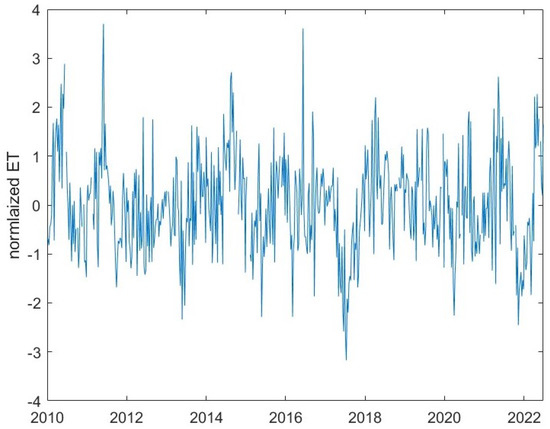
Figure 5.
Normalized residual of pixel time series shown in Figure 2.
We applied the MFDFA to each residual pixel time series, varying the moment order q from −5 to 5 and the scale m from 10 to 1/4 of the length of the series. The gaps were eliminated by simply stitching together the two neighbors [28]. In order to select the optimum degree of the detrending polynomial, we calculated the fluctuation functions for each q for detrending polynomial degree . For each we computed the coefficient of determination of the linear fit of and analyzed the multifractality of those pixels, whose for any q, while those with for at least one value of q were discarded. Figure 6 and Figure 7 show the variation of (average of over all the selected pixels) versus q, for for the infected and not-infected areas, respectively; we can see that is relatively larger for for the areas not affected by Xylella fastidiosa, while it is the largest for for the affected areas. Thus, we analyzed the multifractality with and for the Xylella-affected and Xylella-not-affected areas, respectively. Moreover, with these values of p, the number of selected pixels is 989/996 for the infected area and 1005/1023 for the not-infected area. As an example, Figure 8 and Figure 9 show the fluctuation functions for and of two pixels, the first for an infected site and the other for an uninfected site. Figure 10, Figure 11 and Figure 12 show the boxplots of the multifractal parameters: -range, W, and .
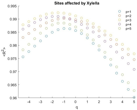
Figure 6.
of the pixels covering the infected area.
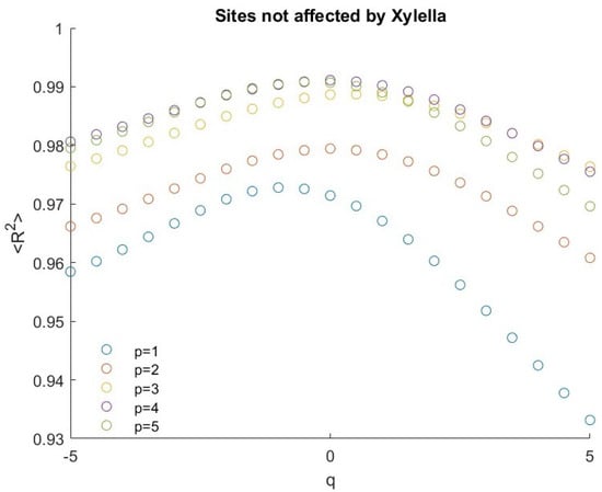
Figure 7.
of the pixels covering the not-infected area.
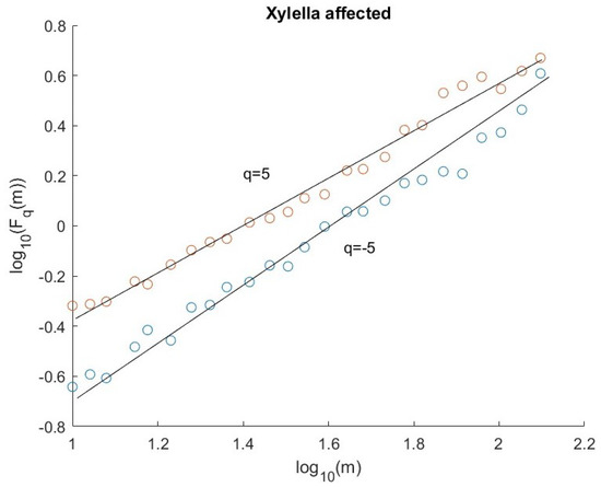
Figure 8.
Fluctuation functions for and of an Xylella-affected pixel.
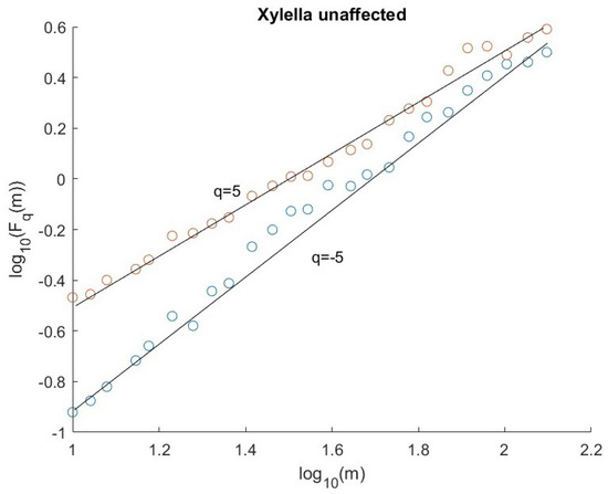
Figure 9.
Fluctuation functions for and of an Xylella-unaffected pixel.
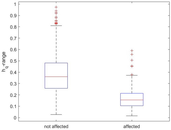
Figure 10.
Boxplot of the -range.
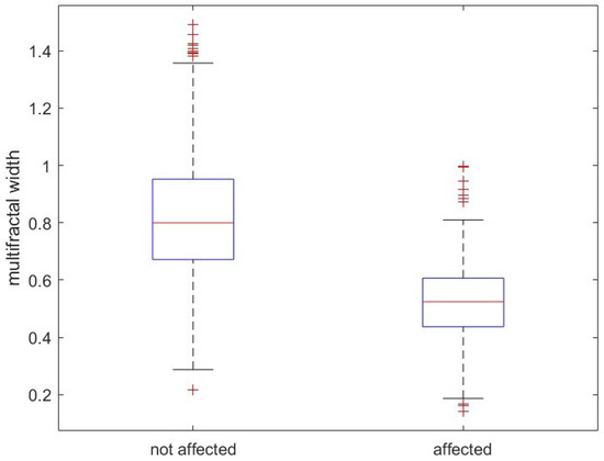
Figure 11.
Boxplot of the width W.
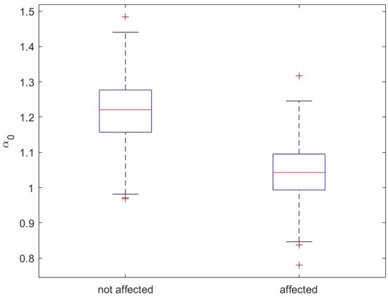
Figure 12.
Boxplot of the maximum .
Moreover, we applied the Fisher–Shannon analysis and calculated the FIM and the for the investigated pixel time series of both types of area. Figure 13 and Figure 14 show the boxplots of the two informational quantities.
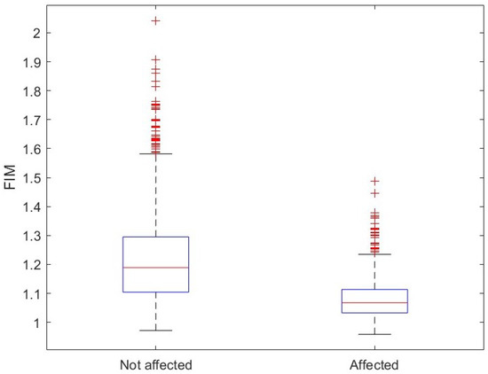
Figure 13.
Boxplot of the FIM.
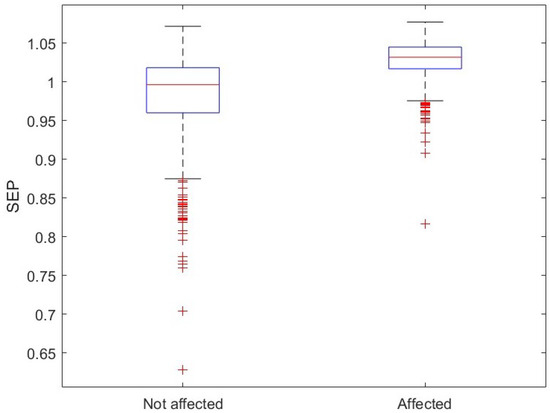
Figure 14.
Boxplot of the SEP.
Table 1 shows the average, the standard deviation, and the minimum and maximum of each multifractal and informational parameter for both the infected and uninfected areas.

Table 1.
Average, standard deviation, and minimum and maximum of the obtained parameters for the Xylella affected (unaffected) sites.
We analyzed the receiver operating characteristic (ROC) curve of each of the three multifractal (-range, W, and ) and of the two informational (FIM and ) parameters to test their performance in discriminating between infected and not-infected olive trees. The ROC curves are well known to test the performance of binary classifiers [24]. The ROC curve shows the relationship between the TPr and the FPr. For each of the five parameters, we constructed the corresponding ROC curve by varying a threshold. Focusing, for instance, on the parameter W that is the width of the multifractal spectrum, there are 989 values for infected pixels (with a mean ) and 1005 for uninfected pixels (with a mean ). W ranges from the minimum 0.1410 to the maximum 1.4920 (see Table 1). The threshold ranges from the minimum to the maximum of all the values of W. After sorting all values of W in increasing order and fixing a threshold F, since , a TP is a value of infected pixel below F, an FP is a value of uninfected pixel below F, an FN is a value of infected pixel above F, and a TN is a value of uninfected pixel above F. Thus, for this value F of the threshold, the TPr and the FPr can be calculated and one point of the ROC curve is obtained. Changing the value of the threshold among all those between the minimum and the maximum and repeating the same procedure, the entire ROC curve is obtained. After cosntructing the ROC curve, the value of the optimal threshold corresponds to the point of the ROC curve that is the closest to (0,1).
Figure 15 shows the ROC curve for the five analyzed parameters. The thresholds corresponding to the point of the ROC curve closest to (0,1) along with the TPr and the FPr for each parameter are reported in Table 2.
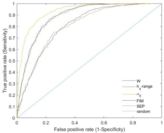
Figure 15.
ROC curves for the five investigated parameters.

Table 2.
Threshold, TPr, and FPr corresponding to the point of the ROC curve closest to (0,1).
Figure 16 shows the corresponding AUC. It is clearly evident that all the parameters can be considered good classifiers and the maximum is the best one.
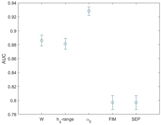
Figure 16.
AUC for the five investigated parameters.
5. Discussion and Conclusions
Recent investigations performed by Telesca et al. [29] showed that MODIS satellite ET, along with other vegetation indices, was effective for assessing the deterioration of pinus tree vegetation by another parasite, Toumeyella parvicornis, suggesting the use of this parameter for the monitoring of pest and parasite attack at both landscape and field scale.
According to [30], Xylella is not the primary cause of the rapid olive desiccation, since the pathogens damage the plants that have been made weaker due to environmental criticalities such as, for example, the reduction of rainfall, the excess of chemical herbicides, the impoverishment of soil organic matter, etc. In this view, these critical factors create an inhospitable environment for the plant, which loses vigor and increases its vulnerability to diseases and parasites, such as Xylella fastidiosa. Thus, ET could characterize and capture the impact of infection by Xylella fastidiosa on plants, since one of the recognizable effects is that the plant dries up and dies. In fact, the ET is well suited to give information about the water status of plants, since it furnishes an indirect measure of the loss of water content of vegetation. Therefore, since the most important symptom of Xylella fastidiosa-induced disease is the rapid desiccation, it is expected that ET makes it possible to detect the presence of this bacterium.
All the investigated sites, both infected and healthy, show a cyclic component in the ET time variability that is very likely linked with the meteo-climatic seasonal cycles. Two periodicities, in particular, are evidenced, the yearly and the semiannual one. The semiannual periodicity appears more powerful for the infected pixels than for the healthy ones; this is probably due the semestral duration of the vector infectivity that generally lasts from May to October.
The application of MFDFA and the Fisher–Shannon method to the time series of pixels covering healthy and Xylella fastidiosa-infected olive groves in southern Italy allowed us to obtain new insights into the time dynamics of ET. The ET time series of the infected sites show an SEP larger and an FIM lower than those of the healthy sites; this indicates that their time variability is characterized by a larger disorder or less organization. Since FIM and SEP relate, respectively, to the local and global properties of the distribution of the series, the larger SEP of the infected sites would suggest that the global variations of their distribution are dominant, while the distribution of the ET series for the healthy sites would be dominated by the local variations.
The two types of sites have different informational response, and this could be correlated to the different nutritional processes that in the infected trees are seriously damaged. The nutritional system of plants is governed by processes that control water and nutrient flux from the roots to the stem and up to the leaves; thus, a healthy tree is characterized by a nutritional system more complex that involves an interaction with the environment. A healthy tree can react more efficiently to the local environmental factors, implying a higher resilience to the external factors that is reflected in a larger heterogeneity, and, thus, in a larger FIM or lower SEP.
In addition, the multifractal parameters -range, multifractal width W, and indicate that the healthy sites are characterized by larger heterogeneity and complexity in the ET time variation. The -range and the width W quantify the variety of the scaling exponents of the series; therefore, large -range and width W indicate that the ET series of healthy sites show a relatively irregular behavior with a variety of scaling exponents larger than that shown by the infected sites that are characterized by a more regular behavior with more homogeneous variations. The maximum of the multifractal spectrum is lower for the infected sites that, therefore, are more regular processes with coarser structure. The larger homogeneity and regularity of the ET of the infected sites could also be an indication of the less resilient behavior versus the local environmental perturbations; in fact, the status of desiccation induced by Xylella fastidiosa makes the nutritional control mechanism of the infected trees less efficient in reacting to the environmental factors, leading, finally, to the death of the infected plant.
The ROC analysis shows the good performance of the five informational and multifractal parameters in discriminating healthy from infected sites but it suggests that the multifractal patterns can be more effective than the informational patterns in ET time series in discerning signs of Xylella fastidiosa infection; furthermore, among the multifractal parameters, the maximum of the multifractal spectrum performs better than the others.
In the future, we aim at enlarging the analysis of these data, focusing, in particular, on two aspects: (1) the application of different classification methods to find the most efficient procedure that allows the best discrimination between healthy and infected sites; and (2) the investigation of the time variation of multifractal and informational parameters in order to better determine the outbreak of the infection. This last point, of course, requires the availability of a dataset much longer than that analyzed in this work. In fact, in order to perform a time-varying analysis, a fixed-length window has to be moved over the entire dataset and the parameters calculated within each window, which has to be large enough to obtain reliable results and smaller enough (compared with the size of the dataset) to have a sufficient number of windows.
However, our results point to the role of ET in contributing to the diagnosis of status of vegetation deterioration due to the attacks of pests and parasites, highlighting the relevance of this parameter as one of the most useful vegetation indices, whose importance has already been assessed in climate change investigations, environmental monitoring and risk estimation, land management, agricultural practices, and food security, thus contributing to the definition of operational tools for the monitoring of biophysical parameters of the vegetation status.
Author Contributions
Conceptualization, L.T. and R.L.; methodology, L.T.; software, M.L.; formal analysis, L.T.; investigation, L.T. and R.L.; resources, R.L.; data curation, F.F. and N.A.; writing—original draft preparation, L.T.; writing—review and editing, L.T. and R.L.; visualization, L.T.; project administration, R.L.; funding acquisition, R.L. All authors have read and agreed to the published version of the manuscript.
Funding
This research was supported by the project COELUM, funded by the National Research Council of Italy.
Data Availability Statement
The data are freely available online (https://lpdaac.usgs.gov) and in the Google Earth Engine (GEE) cloud database.
Conflicts of Interest
The authors declare no conflict of interest.
References
- Pyšek, P.; Hulme, P.; Simberloff, D.; Bacher, S.; Blackburn, T.; Carlton, J.; Dawson, W.; Essl, F.; Foxcroft, L.; Genovesi, P.; et al. Scientists’ warning on invasive alien species. Biol. Rev. 2020, 95, 1511–1534. [Google Scholar] [CrossRef] [PubMed]
- Wallingford, P.; Morelli, T.; Allen, J.; Beaury, E.; Blumenthal, D.; Bradley, B.; Dukes, J.; Early, R.; Fusco, E.; Goldberg, D.; et al. Adjusting the lens of invasion biology to focus on the impacts of climate-driven range shifts. Nat. Clim. Chang. 2020, 10, 398–405. [Google Scholar] [CrossRef]
- Chaloner, T.; Gurr, S.; Bebber, D. Plant pathogen infection risk tracks global crop yields under climate change. Nat. Clim. Chang. 2021, 11, 710–715. [Google Scholar] [CrossRef]
- Sorensen, J.; Gill, R. A range extension of Homalodisca coagulata (Say) (Hemiptera: Clypeorrhyncha: Cicadellidae) to southern California. Pan-Pac. Entomol. 1996, 72, 160–161. [Google Scholar]
- Janse, J.; Obradovic, A. Xylella fastidiosa: Its biology, diagnosis, control and risks. J. Plant Pathol. 2010, 92, S35–S48. [Google Scholar]
- Schneider, K.; van der Werf, W.; Cendoya, M.; Mourits, M.; Navas-Cortés, J.; Vicent, A.; Oude Lansink, A. Impact of Xylella fastidiosa subspecies pauca in European olives. Proc. Natl. Acad. Sci. USA 2020, 117, 9250–9259. [Google Scholar] [CrossRef] [PubMed]
- Hearon, S.; Sherald, J.; Kostka, S. Association of xylem-limited bacteria with elm, sycamore, and oak leaf scorch. Can. J. Bot. 1980, 58, 1986–1993. [Google Scholar] [CrossRef]
- Wells, J. Isolation, culture, and pathogenicity of the bacterium causing phony disease of peach. Phytopathology 1980, 73, 859. [Google Scholar] [CrossRef]
- Saponari, M.; Boscia, D.; Nigro, F.; Martelli, G. Identification of DNA sequences related to Xylella fastidiosa in oleander, almond and olive trees exhibiting leaf scorch symptoms in Apulia (Southern Italy). J. Plant Pathol. 2013, 95, 668. [Google Scholar]
- Jeger, M.; Caffier, D.; Candresse, T.; Chatzivassiliou, E.; Dehnen-Schmutz, K.; Gilioli, G.; Grégoire, J.C.; Jaques Miret, J.; MacLeod, A.; Navajas Navarro, M.; et al. Scientific opinion on the updated pest categorisation of Xylella fastidiosa. EFSA J. 2018, 16, 5357. [Google Scholar]
- Krugner, R.; Sisterson, M.S.; Chen, J.; Stenger, D.C.; Johnson, M.W. Evaluation of olive as a host of Xylella fastidiosa and associated sharpshooter vectors. Plant Dis. 2014, 99, 1186–1193. [Google Scholar] [CrossRef]
- Haelterman, R.M.; Tolocka, P.A.; Roca, M.E.; Guzmán, F.A.; Fernández, F.D.; Otero, M.L. First presumed diagnosis of Xylella fastidiosa causing olive scorch in Argentina. J. Plant Pathol. 2015, 97, 393. [Google Scholar]
- Coletta-Filho, H.D.; Francisco, C.S.; Lopes, J.R.S.; de Oliveira, A.F.; da Silva, L.F.O. First report of olive leaf scorch in Brazil, associated with Xylella fastidiosa subsp. pauca. Phytopathol. Mediterr. 2016, 55, 130–135. [Google Scholar]
- Giampetruzzi, A.; Chiumenti, M.; Saponari, M.; Donvito, G.; Italiano, A.; Loconsole, G.; Boscia, D.; Cariddi, C.; Martelli, G.P.; Saldarelli, P. Draf genome Sequence of Xylella fastidiosa CoDiRO Strain. Genome Announc. 2015, 3, e01538-14. [Google Scholar] [CrossRef] [PubMed]
- Strona, G.; Carstens, C.J.; Beck, P.S. Network analysis reveals why Xylella fastidiosa will persist in Europe. Sci. Rep. 2017, 7, 71. [Google Scholar] [CrossRef] [PubMed]
- Bock, C.; Poole, G.; Parker, P.; Gottwald, T. Plant disease severity estimated visually, by digital photography and image analysis, and by hyperspectral imaging. CRC Crit. Rev. Plant Sci. 2010, 29, 59–107. [Google Scholar] [CrossRef]
- Castrignanó, A.; Belmonte, A.; Antelmi, I.; Quarto, R.; Quarto, F.; Shaddad, S.; Sion, V.; Muolo, M.R.; Ranieri, N.A.; Gadaleta, G.; et al. Semi-Automatic Method for Early Detection of Xylella fastidiosa in Olive Trees Using UAV Multispectral Imagery and Geostatistical-Discriminant Analysis. Remote Sens. 2021, 13, 14. [Google Scholar] [CrossRef]
- Zarco-Tejada, P.; Camino, C.; Beck, P.; Calderon, R.; Hornero, A.; Hernández-Clemente, R.; Kattenborn, T.; Montes-Borrego, M.; Susca, L.; Morelli, M.; et al. Previsual symptoms of Xylella fastidiosa infection revealed in spectral planttrait alterations. Nat. Plant. 2018, 4, 432–439. [Google Scholar] [CrossRef]
- Camino, C.; Calderón, R.; Parnell, S.; Dierkes, H.; Chemin, Y.; Román-Écija, M.; Montes-Borrego, M.; Landa, B.B.; Navas-Cortes, J.A.; Zarco-Tejada, P.J.; et al. Detection of Xylella fastidiosa in almond orchards by synergic use of an epidemic spread model and remotely sensed plant traits. Remote. Sens. Environ. 2021, 260, 112420. [Google Scholar] [CrossRef]
- Frieden, B.R. Fisher information, disorder, and the equilibrium distributions of physics. Phys. Rev. A 1990, 41, 4265–4276. [Google Scholar] [CrossRef]
- Shannon, C.E. A mathematical theory of communication. Bell Syst. Tech. J. 1948, 27, 379–423. [Google Scholar]
- Kantelhardt, J.W.; Zschiegner, S.A.; Konscienly-Bunde, E.; Havlin, S.; Bunde, A.; Stanley, H.E. Multifractal detrended fluctuation analysis of nonstationary time series. Phys. A 2002, 316, 87–114. [Google Scholar]
- Martin, M.; Perez, J.; Plastino, A. Fisher information and nonlinear dynamics. Physica A 2001, 291, 523–532. [Google Scholar]
- Fawcett, T. An introduction to ROC analysis. Pattern Recognit. Lett. 2006, 27, 861–874. [Google Scholar] [CrossRef]
- Saponari, M.; Giampetruzzi, A.; Loconsole, G.; Boscia, D.; Saldarelli, P. Xylella fastidiosa in Olive in Apulia: Where We Stand. Phytopathology 2019, 109, 175–186. [Google Scholar] [CrossRef] [PubMed]
- Laipelt, L.; Kayser, R.H.B.; Fleischmann, A.S.; Ruhoff, A.; Bastiaanssen, W.; Erickson, T.A.; Melton, F. Long-term monitoring of evapotranspiration using the SEBAL algorithm and Google Earth Engine cloud computing ISPRS. J. Photogramm. Remote. Sens. 2021, 178, 81–96. [Google Scholar]
- European Union (EU). Commission Implementing Decision (EU) 2018/927 of 27 June 2018 Amending Implementing Decision (EU) 2015/789 as Regards Measures to Prevent the Introduction into and the Spread within the Union of Xylella fastidiosa (Wells et al.) Notified under Document C (2018) (683 3972). 2018. Available online: https://eur-lex.europa.eu/legal-content/EN/TXT/PDF/?uri=CELEX:32018D0927 (accessed on 25 May 2023).
- Chen, Z.; Ivanov, P.C.; Hu, K.; Stanley, H.E. Effect of nonstationarities on detrended fluctuation analysis. Phys. Rev. E 2002, 65, 041107. [Google Scholar] [CrossRef]
- Telesca, L.; Aromando, A.; Faridani, F.; Lovallo, M.; Cardettini, G.; Abate, N.; Papitto, G.; Lasaponara, R. Exploring Long-Term Anomalies in the Vegetation Cover of Peri-Urban Parks Using the Fisher-Shannon Method. Entropy 2022, 24, 1784. [Google Scholar] [CrossRef] [PubMed]
- Ciervo, M. The olive quick decline syndrome (OQDS) diffusion in Apulia Region: An apparent contradiction according to the agricultural model. Rev. Belg. Geogr. 2016, 4, 1–22. [Google Scholar] [CrossRef]
Disclaimer/Publisher’s Note: The statements, opinions and data contained in all publications are solely those of the individual author(s) and contributor(s) and not of MDPI and/or the editor(s). MDPI and/or the editor(s) disclaim responsibility for any injury to people or property resulting from any ideas, methods, instructions or products referred to in the content. |
© 2023 by the authors. Licensee MDPI, Basel, Switzerland. This article is an open access article distributed under the terms and conditions of the Creative Commons Attribution (CC BY) license (https://creativecommons.org/licenses/by/4.0/).