Article

Sliding-Window TD-FrFT Algorithm for High-Precision Ranging of LFM Signals in the Presence of Impulse Noise

1
School of Optoelectronic Engineering, Xi’an Technological University, Xi’an 710021, China
2
Xi’an Key Laboratory of Active Photoelectric Imaging Detection Technology, Xi’an Technological University, Xi’an 710021, China
*
Authors to whom correspondence should be addressed.
These authors contributed equally to this work.
Fractal Fract. 2023, 7(9), 679; https://doi.org/10.3390/fractalfract7090679
Submission received: 19 June 2023 / Revised: 3 September 2023 / Accepted: 7 September 2023 / Published: 11 September 2023
(This article belongs to the Special Issue Recent Advances in Fractional Fourier Transforms and Applications)

Abstract

:
To address the performance degradation of the conventional linear frequency modulation signal ranging method in the presence of impulse noise, this paper proposes a novel technique that integrates a sliding-window tracking differentiator (TD) with the fractional Fourier transform (FrFT) ranging method. First, the sliding-window TD filtering algorithm is used to suppress the noise in the echo. Subsequently, the filtered signal is subjected to FrFT to calculate the time delay based on the difference in the peak point positions in the fractional domain for realizing target ranging. The simulation results show that the proposed method can effectively suppress impulse noise of different intensities and achieve an accurate and robust ranging of the target.

1. Introduction

The α-stable distribution [1,2,3,4,5,6,7] constitutes a class of impulse signal models that can effectively describe noise with strong impulsive characteristics and heavy-tailed probability density functions, commonly encountered in sonar, radar, and other detection domains; however, the α-stable distribution lacks finite second-order or higher-order statistics. Consequently, the performance of conventional signal parameter estimation methods, such as fractional low-order statistics [8,9], median filtering [10], myriad [11,12,13] filtering, and meridian [14,15,16] filtering, is severely degraded in environments involving impulse noise. In addition, traditional signal processing methods based on the Gaussian model cannot be applied in scenarios involving impulse noise. Although various noise reduction methods based on special cases of α-stable distributions have been proposed, their performance deteriorates under strong impulse noise.
Linear frequency modulation (LFM) signals, which are typical non-stationary signals, are widely used in radar and sonar systems [17,18,19,20,21] for target localization and ranging; therefore, it is of significance to study high-precision ranging methods for LFM signals. The authors of [22] realized the detection and parameter estimation of LFM signals through a time–frequency analysis using short-time Fourier transform and two-dimensional plane search in the time–frequency domain using the Hough transform. However, the performance of this method was noted to degrade in the presence of strong impulse noise; thus, fractional Fourier transform (FrFT) [23] has emerged as a promising tool for time–frequency analysis. Unlike the conventional Fourier transform, FrFT uses the transform order as the independent variable; thus, the LFM signal appears as an impulse signal under the matched FrFT order, resulting in augmented energy aggregation. Consequently, FrFT can be used to estimate the parameters of LFM signals to accomplish target ranging. A previous study [24] proposed an FrFT-based time delay estimation algorithm and compared it with the traditional impulse noise suppression method. The results showed that the FrFT-based time delay estimation algorithm achieved a higher accuracy and efficiency in time delay estimation and could effectively manage more complex operational scenarios. An FrFT-based delay estimation method for LFM signals has also been developed [25]. The method first performs FrFT on the received signal and identifies the peak position as a coarse estimate, then uses the approximate coarse estimate with the theoretical value obtained by the least squares method to achieve a fine estimate of the delay. In another study [26], a multipath delay estimation algorithm for LFM signals was established based on a nonlinear amplitude transform function. The echo and transmitted signals are separately transformed using nonlinear FrFTs, and the delay in the LFM signals is calculated based on the peak position offset in the fractional domain. Other researchers [27,28] have introduced a quantum weighted FrFT for application to quantum singular-value decomposition problems and quantum gradient-solving problems. Moreover, a novel random FrFT has been developed [29], inheriting excellent mathematical properties from the FrFT, which can be directly used in optical image encryption and decryption.
To further suppress impulse noise, a tracking differentiator (TD) filtering algorithm is introduced in this paper. However, the TD filtering algorithm uses a fixed tracking factor to suppress the noise in the echo signal, and therefore has a weak generalization capability and limited application scope. To address this problem, this paper proposes a sliding-window TD filtering algorithm, which can adaptively adjust the tracking factor within a sliding-window, thus enhancing the capability of noise suppression in the echo signal. Following noise suppression, the useful information in the echo signal is extracted by the FrFT, thereby accomplishing accurate target ranging. The results of experimental validation demonstrate that the sliding-window TD-FrFT method outperforms the TD-FrFT method and median-FrFT methods in terms of robustness in strong impulse noise environments.

2. Ranging Principle of LFM Signals Based on FrFT

In the ranging of LFM signals based on FrFT, the FrFT with the optimal order is applied to the transmitted and echo signals separately. Subsequently, the maximum peaks of the transmitted and echo signals are identified in the fractional domain, and the target distance is estimated by converting the difference in the positions of the two peaks in the fractional domain to the time delay. This ranging principle is illustrated in Figure 1.

3. LFM Signal Ranging under Impulse Noise

3.1. TD Filtering Algorithm

Echo signals typically contain large amounts of impulse noise, which can obscure the signals, rendering the FrFT ranging algorithm ineffective in extracting relevant information from echo signals. To address this problem, the concept of TD was introduced [30,31]. By adjusting the TD parameters, noise data can be effectively filtered. Therefore, in this study, the TD method is used to suppress the noise of echo signals.
The architecture of the TD can be summarized as follows. Echo signal v ( t ) is input to the TD, and x 1 ( t ) and x 2 ( t ) signals are obtained as outputs. Here, x 1 ( t ) is the tracking-output signal of v ( t ) , and x 2 ( t ) is the differential signal of v ( t ) .
The discrete form of the TD is as follows:
{ x 1 ( k + 1 ) = x 1 ( k ) + h x 2 ( k ) x 2 ( k + 1 ) = x 2 ( k ) + h f h f h = fhan [ x 1 ( k ) v ( k ) , x 2 ( k ) , r , h 0 ] h 0 = n h
The fastest control synthesis function, indicated by f h = f h a n [ x 1 ( k ) v ( k ) , x 2 ( k ) , r , h 0 ] in Equation (1), is as follows:
{ d = r h 0 d 0 = h 0 d y = x 1 + h 0 x 2 a 0 = d 2 + 8 r | y | a = { x 2 + ( a 0 d ) 2 sign ( y ) , | y | > d 0 x 2 + y h 0 , | y | d 0   fhan   = { r sign ( a ) , | a | > d r a d , | a | < d
where, r is the tracking factor; h is the integration step; s i g n · represents the sign function; h 0 is the filtering factor; and n is the filtering coefficient, n 1 .
The TD performs filtering by adjusting the tracking and filtering factors. The tracking factor regulates the rate at which the output data track the input data. A higher tracking factor means that the output data more rapidly track the input data. In scenarios involving noise, the input data are filtered by adjusting the filtering factor; however, as the filtering factor increases, the phase loss of the output data tracking the input data increases as well.

3.2. Sliding-Window TD Filtering Algorithm

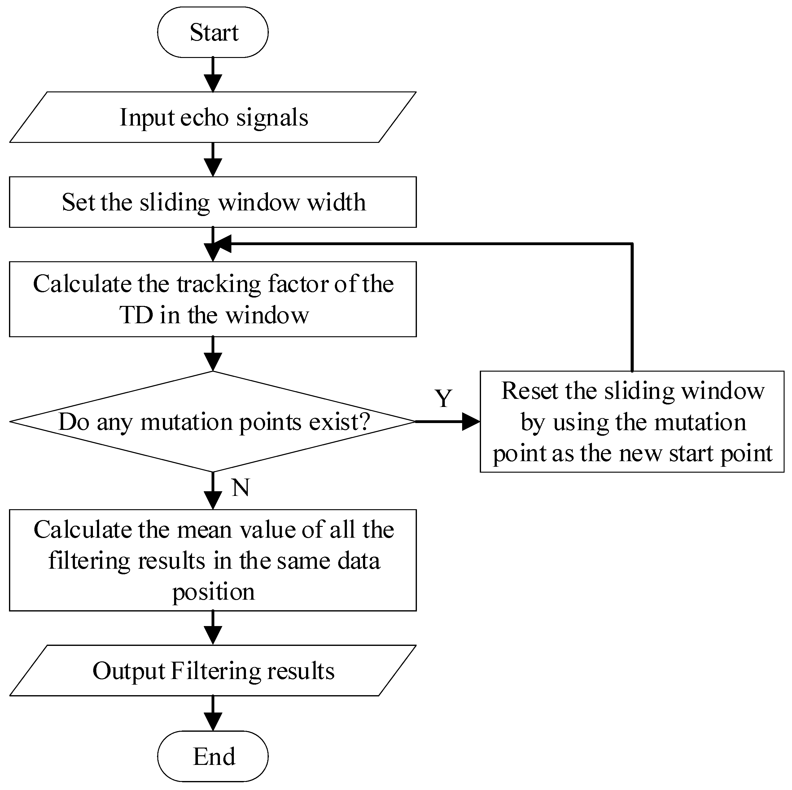
In practical applications, the TD filtering algorithm uses a fixed tracking factor to suppress the noise in echo signals. However, the method exhibits limitations when faced with varying degrees of impulse noise interference, resulting in suboptimal noise suppression [32]. To solve this problem, the paper proposes a sliding-window TD filtering algorithm. This algorithm divides the echo signals into several windows according to the sliding-window principle. Subsequently, the tracking factor is adaptively adjusted according to the stability of the echo signal data in each window to address impulse noise interference from various sources, thereby effectively and efficiently suppressing the impulse noise in the echo signal. The process flow of the algorithm is shown in Figure 2.
When the echo signals are segmented according to the sliding-window principle, the sliding-window width determines the relative stability of the data in each window. This stability is represented by the standard deviation of the data in each window. The process of the sliding-window TD filtering algorithm can be summarized as follows:
First, the sliding-window width is set, and the threshold of the mutation point within the window is calculated, as shown in Equation (3):
T w = λ σ
where, T w is the threshold value of the mutation point within the window; σ is the standard deviation of the data within the sliding-window; and λ is the extraction coefficient of the threshold value of the mutation point, set as three according to the 3σ criterion.
Second, assuming that each mutation point is distributed according to the maximum frequency, the maximum frequency in the window can be determined as follows:
f w = w W
where, f w is the maximum frequency value in the sliding-window. w is the number of data points in the sliding-window with amplitudes exceeding the threshold value of the mutation point. These mutation points are treated as repeated equivalent data. W is the total number of data points.
Third, the tracking factor is adaptively adjusted, yielding the following expression:
r w = ( 1 + σ f w ) r
where, r is the fixed tracking factor, and r w is the tracking factor within the sliding-window.
Fourth, to reduce the influence of noise on the standard deviation of the data within the window, the technique of locally normalized standard deviation is used. This method can effectively reduce the influence of noise on the standard deviation, enabling more accurate calculation of the tracking factor of the data within the sliding-window. Specifically, the average value of the data within the window is used to normalize the standard deviation as follows:
σ w = σ | m w |
where, m w is the mean of the data within the sliding-window, and σ w is the normalized standard deviation.
By substituting the locally normalized standard deviation in Equation (6) into Equation (5), the following expression can be obtained to determine the tracking factor:
r w = ( 1 + | m w | σ w f w ) r
Fifth, to enhance the suppression of noise in the echo signal, it is necessary to filter out the potential mutation points after processing the echo signals with the TD. A mutation point represents a high-amplitude impulse noise point that persists even after the echo signals have been processed by the TD. The presence of these points can increase the errors in the filtering results, and thus, they must be eliminated. The mutation point is identified by setting a threshold value, and it is used as the starting point of the sliding-window.
Finally, through iterative sliding-window filtering, the mean value for the filtered data position is output. This strategy prevents discontinuities in the filtering results, ensuring data continuity.

3.3. FrFT Ranging Algorithm

The p-order FrFT is a linear integration operation defined in the t-domain function x(t). Specifically, the p-order FrFT of signal x(t) can be formulated as follows:
X p ( u ) = F p [ x ( t ) ] = x ( t ) K p ( t , u ) d t
Let A α = 1 j c o t α , n = 1 , 2 , . Then, the kernel function Kp(t,u) can be defined as in Equation (9):
K p ( t , u ) = { A α exp ( j π ( t 2 + u 2 ) cot α j 2 π u t csc α ) α n π δ ( t u ) α = 2 n π δ ( t + u ) α = ( 2 n + 1 ) π
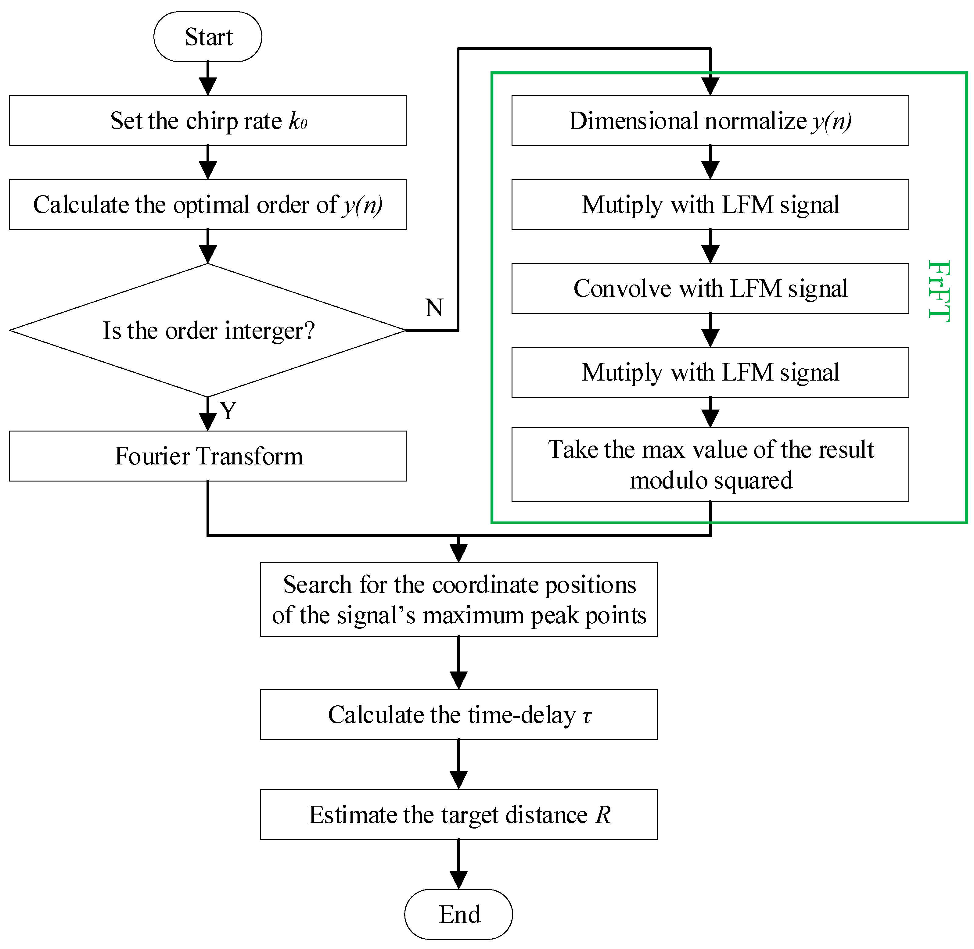
where, φ = π 2 p is the rotation angle of the time–frequency plane, p is the order of the FrFT, F p is the FrFT operator, and δ ( t ) is the unit impulse function. The LFM signals exhibit different degrees of energy aggregation depending on the order in the fractional domain. By leveraging this property, the FrFT method can estimate the parameters of the LFM signals for ranging. According to the expression of the FrFT, the algorithm is decomposed into the convolutional signal form, and the fast Fourier transform is then used to implement the FrFT ranging algorithm. The process flow of the FrFT ranging algorithm is shown in Figure 3.
The optimal order of the FrFT of the echo signal y ( n ) is calculated using the chirp rate k 0 of the transmitted signal x ( n ) . When the optimal order is not an integer, the following steps are implemented:
Multiply the LFM signal exp ( j π n 2 tan φ 2 ) with y ( n ) , i.e., the LFM signal to be ranged:
g ( n ) = exp ( j π n 2 tan φ 2 ) y ( n )
Convolve g ( n ) obtained using exp ( j π n 2 csc φ ) to obtain the following LFM signal:
h ( u ) = A φ ^ exp [ j π csc φ ( u n ) 2 g ( n ) ] d n
Multiply exp ( j π u 2 tan φ 2 ) by h ( u ) :
Y p ( u ) = exp ( j π u 2 tan φ 2 ) h ( u )
Select the maximum value of Y p ( u ) in terms of its squared modulus:
{ p ^ , u ^ } = arg   max ( p , u ) | Y p ( u ) | 2
The FrFT process of the echo signal y ( n ) is presented in the green frame. First, FrFT with the optimal order is performed on the echo signal y ( n ) , and the maximum value in the fractional domain, corresponding to the coordinate position u 1 , is determined. Subsequently, a p-order FrFT is performed on the transmit signal x ( n ) , and the maximum peak point in the u-domain, corresponding to the coordinate position u 2 , is identified. Finally, the time delay τ is calculated as the difference in the two peak positions to measure the target distance R .
R = τ c 2 = ( u 1 u 2 ) sec α k 0 c 2

4. Simulation-Based Experiments and Analysis

The LFM signal can be mathematically modeled as shown in Equation (15):
x ( n ) = A exp ( j 2 π f 0 t + j π k 0 t 2 ) , n [ 0 , T ]
where, A , f 0 , k 0 , and T represent the amplitude, initial frequency, chirp rate, and time width of the signal, respectively. Given the lack of a uniform probability density expression for the α-stable distribution, it is typically described using the characteristic function, as shown in Equation (16):
φ ( t ) = exp { j a t γ | t | α [ 1 + j β sgn ( t ) ω ( t , α ) ] }
ω ( t , α ) = { 2 π lg | t | , α = 1 tan α π 2 , α 1
sgn ( t ) = { 1 , t > 0 0 , t = 0 1 , t < 0
In Equation (16), s g n ( t ) is the sign function; and α is the characteristic parameter, which takes values ranging from 0 to 2. This parameter determines the impulse intensity of the α -stable distribution as follows: a smaller α corresponds to a higher impulse intensity. β is the symmetry parameter, which determines the slope of the α -stable distribution. When β = 0 , the α -stable distribution is symmetric (SαS). γ is the dispersion coefficient, which reflects the degree of dispersion. a is the location parameter. For a standard α -stable distribution, a = 0 and γ = 1 . In this study, SαS is used to model the noise. Because the α -stable distribution lacks second-order statistics, no variance exists. Thus, the generalized signal-to-noise ratio (GSNR) is used, instead of the conventional signal-to-noise ratio, as defined in Equation (19):
G S N R = 10 lg ( σ s 2 / γ )
where, σ s 2 denotes the variance of the signal, and γ is the dispersion coefficient of the noise.
Experiment 1.
Performance verification of the median filtering, TD filtering, and sliding-window TD filtering algorithm.
The performance of three filtering algorithms is evaluated under the same noise conditions in this experiment. The parameters used in the experiment are listed in Table 1.
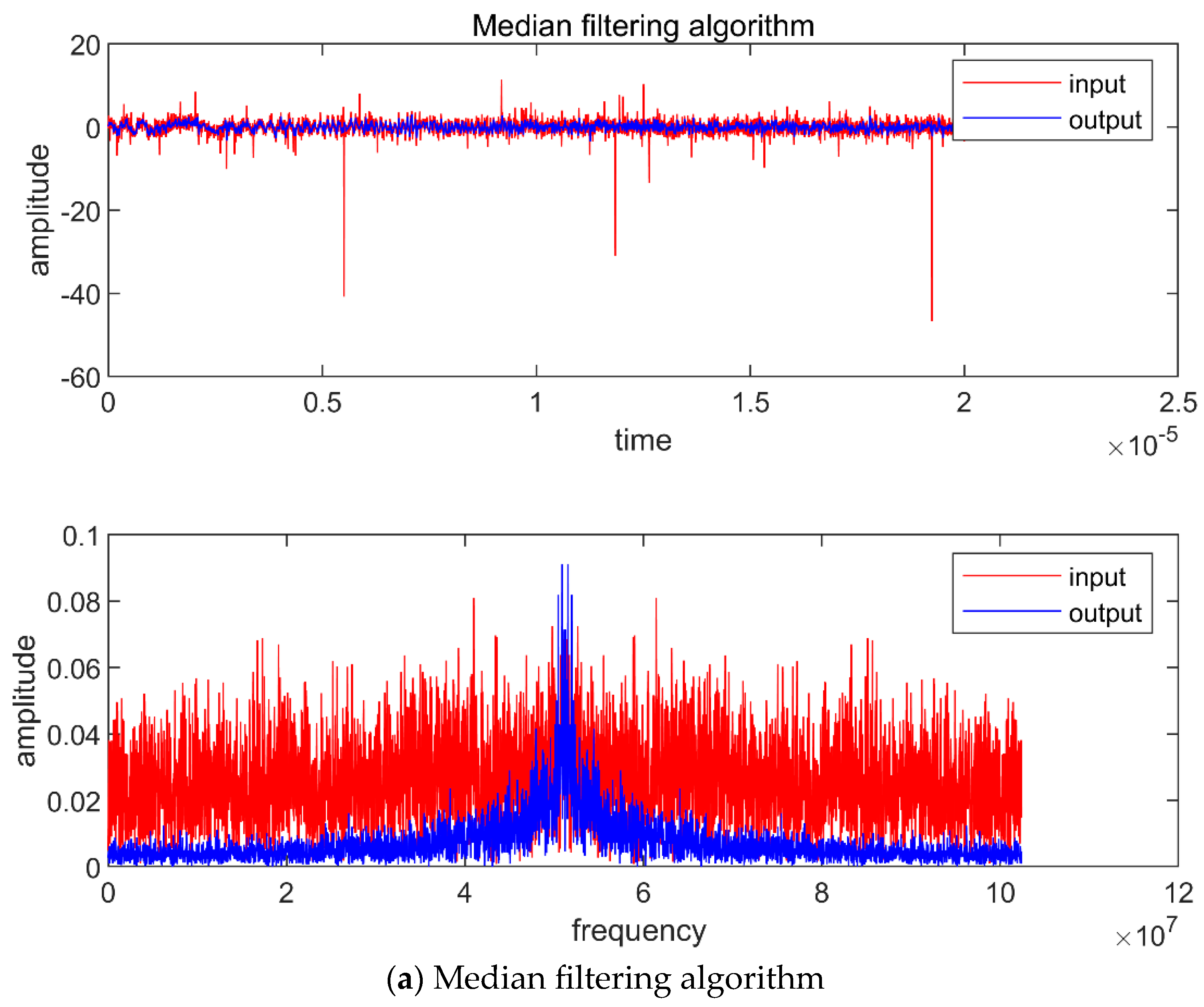
The simulation results of the three algorithms are shown in Figure 4.
Although the median filtering algorithm can effectively suppress impulse noise, it distorts the characteristic information of the echo signal, as shown in Figure 4a. Conversely, the TD filtering algorithm and sliding-window TD filtering algorithm can retain the characteristic information of the echo signal while effectively suppressing the impulse noise. Compared with the TD filtering algorithm, the sliding-window TD filtering algorithm better suppresses the impulse noise and achieves a higher accuracy, as shown in Figure 4b,c.
Experiment 2.
Performance analysis of the median filtering, TD filtering, and sliding-window TD filtering algorithms in terms of the root mean square error (RMSE).
Monte Carlo experiments with 1000 runs are conducted to evaluate the performance of the three algorithms under different α in this experiment. The parameters used in the experiment are listed in Table 2.
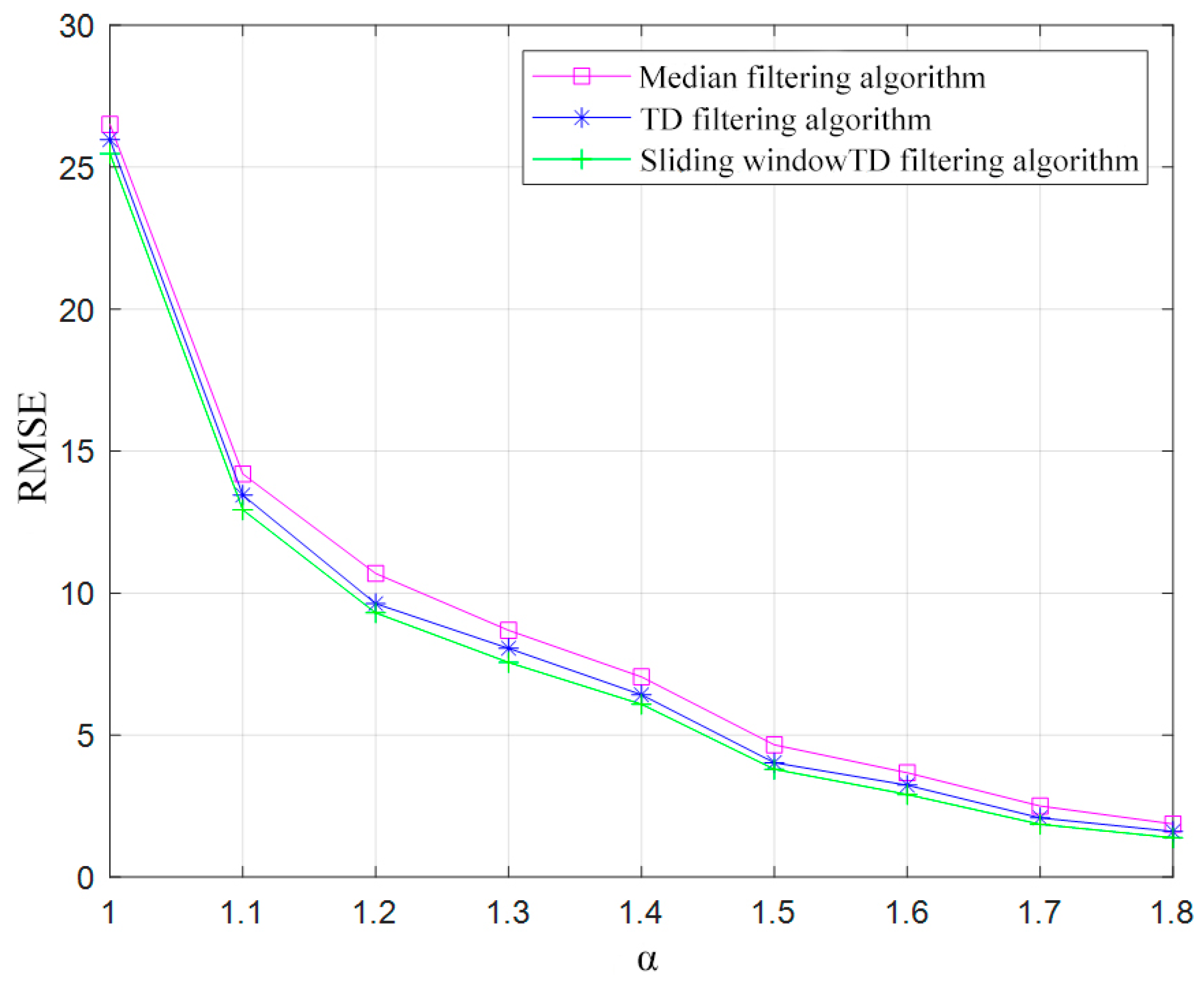
The RMSE values for the three algorithms at different values of α are shown in Figure 5.
The RMSEs of all three algorithms decrease as the impulse intensity decreases, with larger feature factor values in the range of 1.0 α 1.8 and G S N R = 1   d B . Compared with the median filtering and TD filtering algorithms, the sliding-window TD filtering algorithm achieves a smaller RMSE, which indicates its superior performance in suppressing impulse noise and its higher robustness.
Experiment 3.
Filtering performance analysis of the median filtering, TD filtering, and sliding-window TD filtering algorithms under different GSNRs.
Monte Carlo experiments with 1000 runs are conducted to evaluate the performance of the three algorithms under different GSNRs in this experiment. The parameters used in the experiment are listed in Table 3.
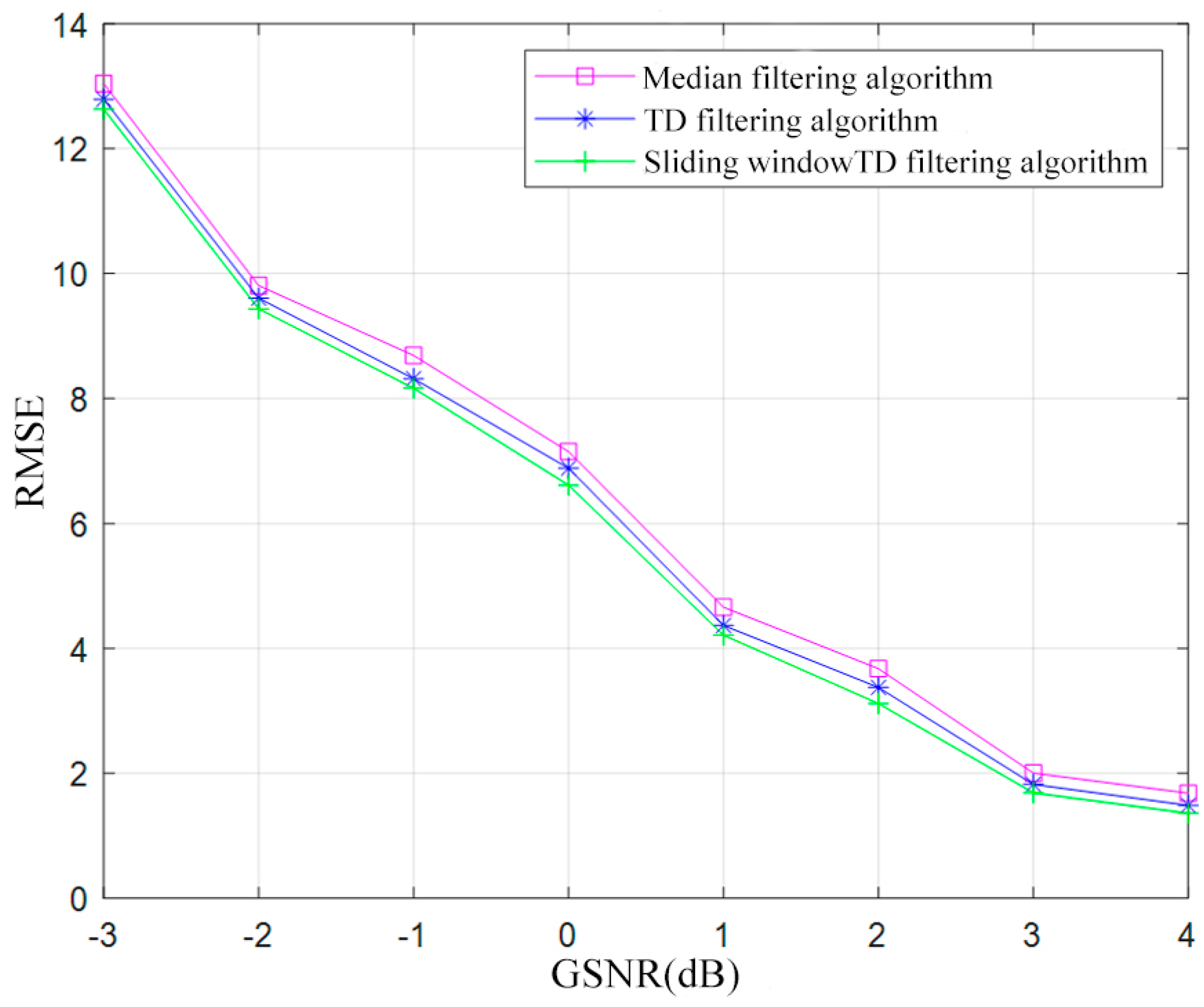
Figure 6 shows the RMSE values of the three algorithms under different GSNRs.
When α = 1.5 , the GSNRs range from −3 dB to 4 dB. The RMSEs of all three algorithms decrease as the GSNR increases, and the intensity of the impulse noise decreases. The sliding-window TD filtering algorithm achieves a smaller RMSE than the TD filtering and median filtering algorithms, which indicates its superior noise suppression ability and performance.
Experiment 4.
Performance comparison of FrFT algorithm, median-FrFT algorithm, TD-FrFT algorithm, and sliding-window TD-FrFT algorithm in the presence of α -stable distribution noise.
The performance of four algorithms in the presence of α-stable distribution noise is evaluated in this experiment. The parameters used in the experiment are listed in Table 4.
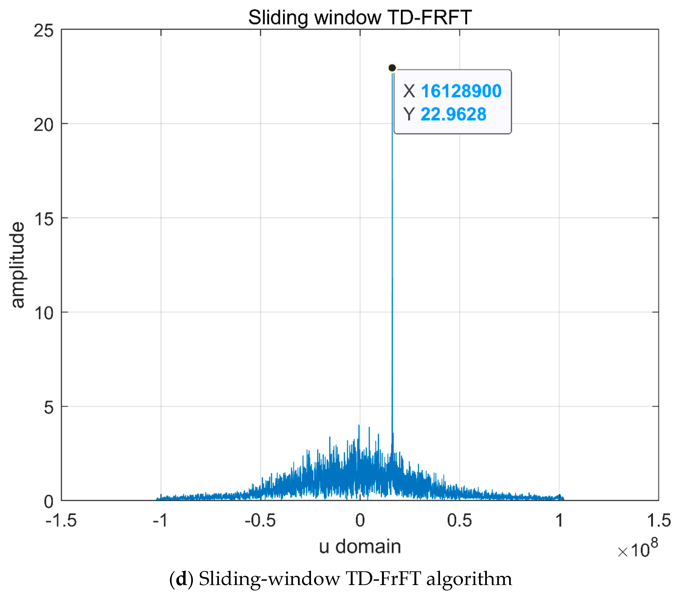
The simulation results of the four algorithms are shown in Figure 7.
The FrFT algorithm is noted to be effective under the considered noise condition, and the useful information from the echo signals can be successfully extracted for ranging. Furthermore, the TD-FrFT algorithm and sliding-window TD-FrFT algorithm exhibit superior filtering performance compared with the median-FrFT algorithm.
Experiment 5.
Ranging performance analysis of FrFT algorithm, median-FrFT algorithm, TD-FrFT algorithm, and sliding-window TD-FrFT algorithm in the presence of SαS distribution noise.
The ranging accuracies of the four algorithms in the presence of noise with different α are compared in this experiment. The parameters used in the experiment are listed in Table 5.
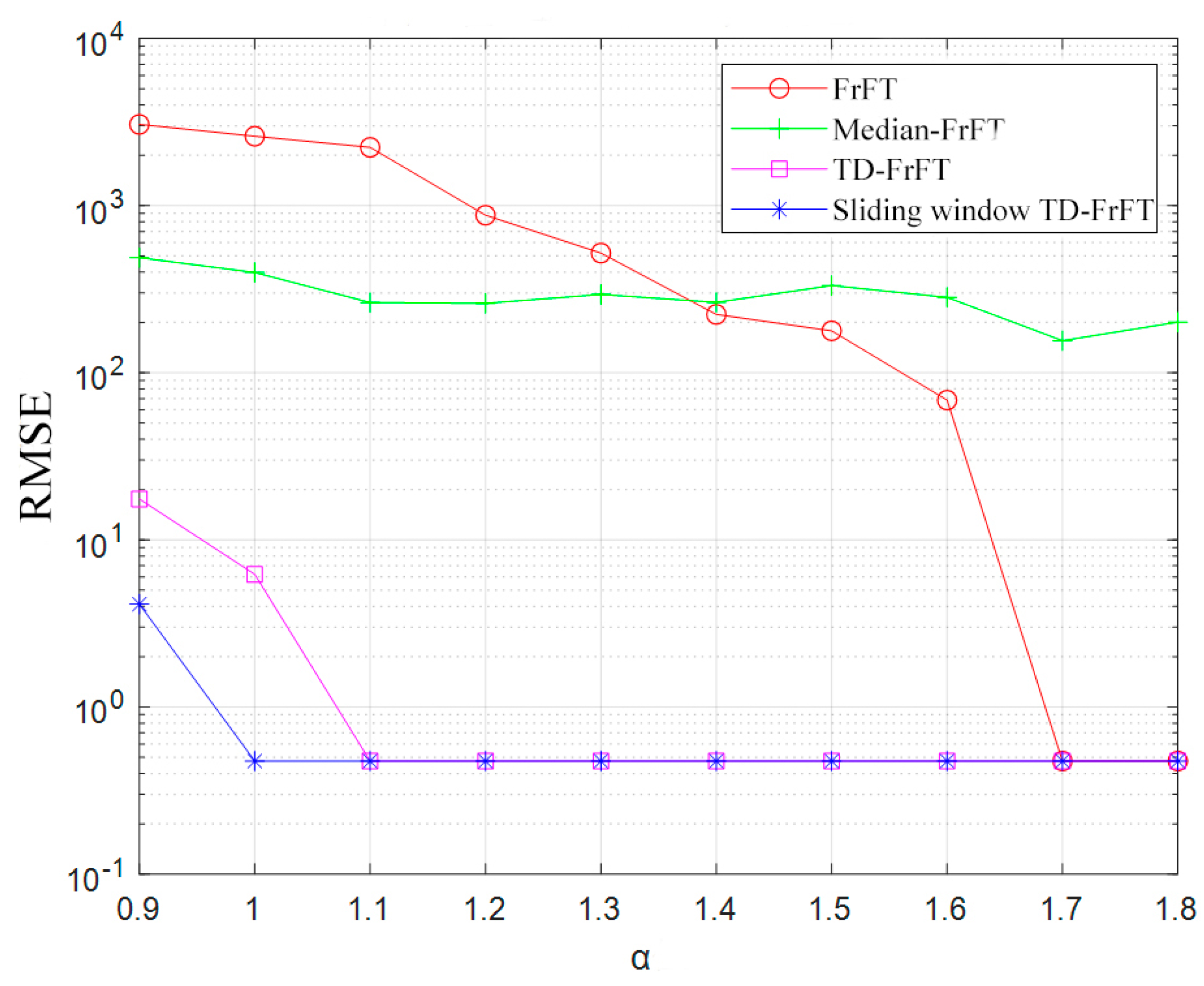
The RMSE values of the four algorithms are shown in Figure 8.
After 1000 Monte Carlo runs, the FrFT algorithm maintains its effectiveness until α = 1.7. At lower values of α, the impulse intensity is low, enabling accurate target ranging. When α < 1.7, the performance of the algorithm degrades. Although the median-FrFT algorithm can effectively suppress the impulse noise, it changes the characteristic information of the echo signal and leads to a shift in the peak position of the echo signal. Even at α = 1.8, the error is too large to achieve effective ranging. The performance of the TD-FrFT algorithm is superior to that of the FrFT algorithm. In the range of 1.1 < α < 1.8, the TD-FrFT algorithm can effectively suppress the impulse noise and determine the target distance. However, the algorithm appears to fail at α < 1.0. When 1.0 < α < 1.8 and GSNR = 1 dB, the error of the sliding-window TD-FrFT algorithm is approximately 0.4748 m, while the average estimated distance is 267.5252 m, which proves that the algorithm can effectively suppress the impulse noise while maintaining a certain estimation accuracy with high robustness.

5. Conclusions

The objective of this study is to address the performance degradation of the traditional LFM signal ranging method in the presence of impulse noise. Specifically, a novel method is introduced to effectively estimate the target distance in the presence of impulse noise. First, the TD algorithm is used to filter the echo signals with noise. Subsequently, the useful information from the noisy echo signals is extracted using FrFT and used for ranging. Simulation results show that the sliding-window TD filtering algorithm can suppress impulse noise with different intensities while maintaining a reasonable ranging accuracy, thereby outperforming the TD filtering algorithm. The results demonstrate the excellent robustness of the proposed method to impulse noise.

Author Contributions

Conceptualization, X.L. and B.X.; methodology, X.L. and B.X.; software, X.L. and B.X.; validation, X.L. and B.X.; formal analysis, X.L. and B.X.; investigation, T.H. and X.L. and B.X.; resources, C.W.; data curation, Y.W.; writing—original draft preparation, X.L., T.H. and B.X.; writing—review and editing, X.L., T.H. and B.X.; visualization, B.X. and X.L.; supervision, C.W.; project administration, C.W.; funding acquisition, C.W. All authors have read and agreed to the published version of the manuscript.

Funding

This research was funded by the National Key R&D Program of China, grant number 2022YFC3803702.

Institutional Review Board Statement

Not applicable.

Informed Consent Statement

Not applicable.

Data Availability Statement

Data underlying the results presented in the paper are not publicly available at this time but may be obtained from the authors upon reasonable request.

Conflicts of Interest

The authors declare no conflict of interest.

References

  1. Talebi, S.P.; Mandic, D.P. Distributed particle filtering of α-stable signals. IEEE Signal Process. Lett. 2017, 24, 1862–1866. [Google Scholar] [CrossRef]
  2. Royuela-del-Val, J.; Simmross-Wattenberg, F.; Alberola-López, C. Libstable: Fast, Parallel, and High-Precision Computation of α-Stable Distributions in R, C/C++, and MATLAB. J. Stat. Soft. 2017, 78, 1–25. [Google Scholar] [CrossRef]
  3. Borijindargoon, N.; Ng, B.P. Directional Adaptive MUSIC-Like Algorithm Under Symmetric α-Stable Distributed Noise. Prog. Electromagn. Res. Lett. 2019, 87, 29–37. [Google Scholar] [CrossRef]
  4. Castillo-Barnes, D.; Martinez-Murcia, F.J.; Ramírez, J.; Górriz, J.M.; Salas-Gonzalez, D. Expectation–Maximization algorithm for finite mixture of α-stable distributions. Neurocomputing 2020, 413, 210–216. [Google Scholar] [CrossRef]
  5. Piotr, K.; Radosław, Z.; Jerome, A.; Agnieszka, W. Generalized spectral coherence for cyclostationary signals with α-stable distribution. Mech. Syst. Signal Process. 2021, 159, 107737. [Google Scholar]
  6. Pelekanakis, K.; Chitre, M. Adaptive Sparse Channel Estimation under Symmetric alpha-Stable Noise. IEEE Trans. Wirel. Commun. 2014, 13, 3183–3195. [Google Scholar] [CrossRef]
  7. Chavali, V.G.; Silva, C.R.C.M.D. Detection of Digital Amplitude—Phase Modulated Signals in Symmetric Alpha-Stable Noise. IEEE Trans. Commun. 2012, 60, 3365–3375. [Google Scholar] [CrossRef]
  8. Feng, P.; Zhang, L.; Meng, D.; Pi, X. An active noise control algorithm based on fractional lower order covariance with on-line characteristics estimation. Mech. Syst. Signal Process. 2023, 186, 109835. [Google Scholar] [CrossRef]
  9. Tao, Y.; Juanatas, R.; Caballero, J.M. Research on a new constant modulus blind equalization algorithm in the mine industrial network. In Proceedings of the 2022 14th International Conference on Communication Software and Networks (ICCSN), Chongqing, China, 10–12 June 2022; pp. 157–160. [Google Scholar] [CrossRef]
  10. Xu, Q.; Cha, D. Research on Signal Processing of Median Filter Method in Vibration Measure for Alpha Stable Distribution Noise. Coal Mine Machinery. 2009, 30, 42–45. [Google Scholar]
  11. Ramirez, J.M.; Paredes, J.L. Recursive weighted myriad based filters and their optimizations. IEEE Trans. Signal Process. 2016, 64, 4027–4039. [Google Scholar] [CrossRef]
  12. Zorlu, H. Optimization of weighted myriad filters with differential evolution algorithm. AEU-Int. J. Electron. Commun. 2017, 77, 1–9. [Google Scholar] [CrossRef]
  13. Liao, X.; Lei, Y.; Luo, L.; Huang, J. An MQAM signal number element rate estimation method based on RHMy filtering under alpha-stable distribution. Signal Process. 2018, 34, 592–601. [Google Scholar]
  14. Kurkin, D.; Roenko, A.; Lukin, V.; Djurovič, I. An adaptive meridian estimator. In Proceedings of the 2011 Microwaves, Radar and Remote Sensing Symposium, Kiev, Ukraine, 25–27 August 2011; pp. 301–304. [Google Scholar] [CrossRef]
  15. Pander, T.; Przybyła, T. Impulsive noise cancelation with simplified Cauchy-based p-norm filter. Signal Process. 2012, 92, 2187–2198. [Google Scholar] [CrossRef]
  16. Jin, Y.; Hu, B.X.; Ji, H.B. A unified framework for robust weighted filtering under α-stable distributed noise. Syst. Eng. Electron. Technol. 2016, 38, 2221–2227. [Google Scholar]
  17. Jin, Y.; Duan, P.T.; Ji, H.B. Parameter Estimation of LFM Signals Based on LVD in Complicated Noise Environments. J. Electron. Inf. 2014, 36, 1106–1112. [Google Scholar]
  18. Zhu, X.; Xu, S.; Zhang, Z.; Xu, X.; Zhang, X. Signal processing algorithm for multi-target underwater positioning system. Foreign Electron. Meas. Technol. 2020, 39, 19–24. [Google Scholar]
  19. Zhao, Z.K.; Gong, H.; Zhang, R. A method for radiation source signal detection based on sequential statistical filtering and binary accumulation. Syst. Eng. Electron. Technol. 2022, 44, 1085–1092. [Google Scholar]
  20. Duan, H.; Cheng, Y.; Shen, B.; Bai, G. LFM interference cancellation algorithm based on MDPT-WC for mark XIIA mode 5. In Proceedings of the 2020 IEEE 20th International Conference on Communication Technology (ICCT), Nanning, China, 28–31 October 2020; IEEE: Piscataway, NJ, USA, 2020; pp. 246–252. [Google Scholar]
  21. Shangguan, J.X.; Zhang, S.Q.; Zheng, L.J.; Jiang, A.Q.; Ai, H.K.; Zhang, L.G.; Liu, H.T. Signal denoiseing method based on regularized chirp mode pursuit algorithm and its applications. Acta Metrol. Sin. 2022, 43, 798–804. [Google Scholar]
  22. Zhang, X. Modern Signal Processing; Tsinghua University Press: Beijing, China, 1995. [Google Scholar]
  23. Tao, R.; Li, X.M.; Li, Y.L.; Wang, Y. Time-delay estimation of chirp signals in the fractional Fourier domain. IEEE Trans. Signal Process. 2009, 57, 2852–2855. [Google Scholar]
  24. Li, X.; Li, L.; Jiang, Y. DFrFT-based pulse pressure method and performance comparison with matched filtering. Comput. Eng. Appl. 2012, 48, 16–21. [Google Scholar]
  25. Yang, C.; Yu, Y.; Wu, C.; Ning, G. A fast time-delay estimator for linear frequency modulation signal based on FrFT. In Proceedings of the 2019 IEEE 3rd Information Technology, Networking, Electronic and Automation Control Conference (ITNEC), Chengdu, China, 15–17 March 2019; IEEE: Piscataway, NJ, USA, 2019; pp. 2278–2281. [Google Scholar]
  26. Chen, M.; Hsing, H.Y.; Wang, H.F. Multipath time delay estimation of LFM signals based on NAT function under impulse noise. J. Electron. Meas. Instrum. 2022, 36, 73–81. [Google Scholar]
  27. Zhao, T.; Chi, Y. Quantum Weighted Fractional-Order Transform. Fractal Fract. 2023, 7, 269. [Google Scholar] [CrossRef]
  28. Zhao, T.; Chi, Y. Multiweighted-Type Fractional Fourier Transform: Unitarity. Fractal Fract. 2021, 5, 205. [Google Scholar] [CrossRef]
  29. Wang, Z.; Long, Z.; Xie, Y.; Ding, J.; Luo, J.; Li, X. A Discrete Nonlinear Tracking-Differentiator and Its Application in Vibration Suppression of Maglev System. Math. Probl. Eng. 2020, 2020, 1849816. [Google Scholar] [CrossRef]
  30. Liu, Z.J.; Liu, S.T. Random fractional Fourier transform. Opt. Lett. 2007, 32, 2088–2090. [Google Scholar] [CrossRef]
  31. Liu, X.L.; Li, X.; Xiao, B.; Wang, C.Y.; Ma, B. LFM Signal Parameter Estimation via FTD-FRFT in Impulse Noise. Fractal Fract. 2023, 7, 69. [Google Scholar] [CrossRef]
  32. Zhang, K.; Jiang, H.X.; Wang, J.Y. A filtering method for telemetry data based on sliding maximum velocity tracking differentiator. J. Northwestern Polytech. Univ. 2020, 38, 515–522. [Google Scholar] [CrossRef]
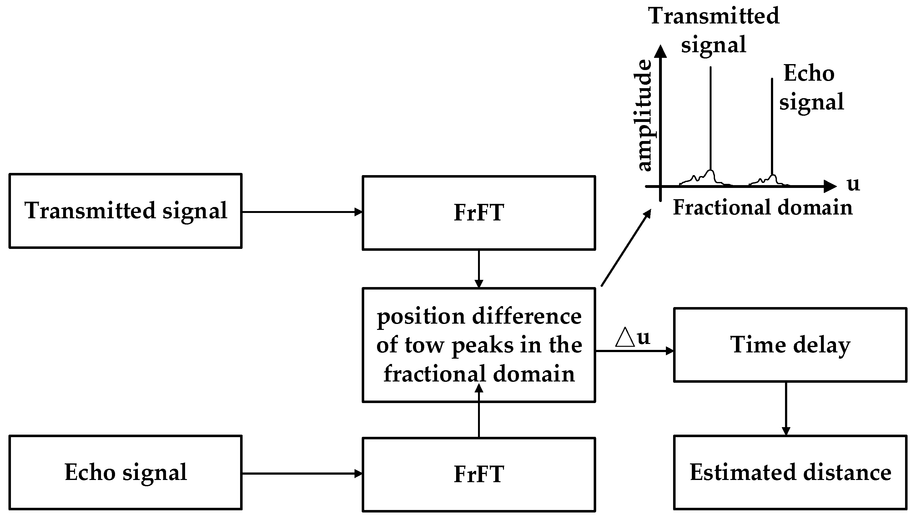
Figure 1. Ranging principle of LFM signals based on FrFT.
Fractalfract 07 00679 g001
Figure 2. Process flow of the sliding-window TD filtering algorithm.
Fractalfract 07 00679 g002
Figure 3. Process flow of the FrFT ranging algorithm.
Fractalfract 07 00679 g003
Figure 4. Simulation results obtained using three algorithms when α = 1.5 and G S N R = 1   d B .
Fractalfract 07 00679 g004aFractalfract 07 00679 g004b
Figure 5. RMSEs corresponding to different α values.
Fractalfract 07 00679 g005
Figure 6. RMSEs corresponding to different GSNRs.
Fractalfract 07 00679 g006
Figure 7. Simulation results of the four algorithms.
Fractalfract 07 00679 g007aFractalfract 07 00679 g007bFractalfract 07 00679 g007c
Figure 8. RMSEs of the range determined by the algorithms corresponding to different α values.
Fractalfract 07 00679 g008
Table 1. Parameters used in Experiment 1.
CategoryNameValueRemarks
Signal parametersA (Amplitude)1 mVThese parameters are arbitrarily set and can be changed according to the practical application.
f0 (Initial frequency)10 Hz
T (Time width of the signal)20 μs
B (Bandwidth)40 MHz
N (Number of sampling points)4096
Noise parametersGSNR1 dBIn this noise condition, the performance of the three algorithms considerably differ.
a (Location parameter)0
α (Characteristic parameter)1.5
β (Symmetry parameter)0
Algorithm parametersr (Tracking factor)10,000This condition corresponds to the optimal TD performance.
h (Step size)0.01
Sliding-window width50
Table 2. Parameters used in Experiment 2.
CategoryNameValueRemarks
Signal parametersA (Amplitude)1 mVThese parameters are the same as those in Experiment 1.
f0 (Initial frequency)10 Hz
T (Time width of the signal)20 μs
B (Bandwidth)40 MHz
N (Number of sampling points)4096
Noise parametersGSNR1 dBIn this noise condition, the performance of three algorithms is analyzed with the α changed.
a (Location parameter)0
α (Characteristic parameter)1.0, 1.1, 1.2, 1.3, 1.4, 1.5, 1.6, 1.7, 1.8
β (Symmetry parameter)0
Algorithm parametersr (Tracking factor)10,000These parameters are the same as those in Experiment 1.
h (Step size)0.01
Sliding-window width50
Table 3. Parameters used in Experiment 3.
CategoryNameValueRemarks
Signal parametersA (Amplitude)1 mVThese parameters are the same as those in Experiment 1.
f0 (Initial frequency)10 Hz
T (Time width of the signal)20 μs
B (Bandwidth)40 MHz
N (Number of sampling points)4096
Noise parametersGSNR−3, −2, −1, 0, 1, 2, 3, 4 (dB)In this noise condition, the performance of three algorithms is analyzed with the GSNR changed.
a (Location parameter)0
α (Characteristic parameter)1.5
β (Symmetry parameter)0
Algorithm parametersr (Tracking factor)10,000These parameters are the same as those in Experiment 1.
h (Step size)0.01
Sliding-window width50
Table 4. Parameters used in Experiment 4.
CategoryNameValueRemarks
Signal parametersA (Amplitude)1 mVAll the parameters are the same as those in Experiment 1.
f0 (Initial frequency)10 Hz
T (Time width of the signal)20 μs
B (Bandwidth)40 MHz
N (Number of sampling points)4096
Noise parametersGSNR1 dB
a (Location parameter)0
α (Characteristic parameter)1.5
β (Symmetry parameter)0
Algorithm parametersr (Tracking factor)10,000
h (Step size)0.01
Sliding-window width50
Table 5. Parameters used in Experiment 5.
CategoryNameValueRemarks
Signal parametersA (Amplitude)1 mVThese parameters are the same as those in Experiment 1.
f0 (Initial frequency)10 Hz
T (Time width of the signal)20 μs
B (Bandwidth)40 MHz
N (Number of sampling points)4096
Noise parametersGSNR1 dBIn this noise condition, the ranging accuracy of three algorithms is analyzed with the α changed.
a (Location parameter)0
α (Characteristic parameter)1.8, 1.7, 1.6, 1.5, 1.4, 1.3, 1.2, 1.1, 1.0, 0.9
β (Symmetry parameter)0
Algorithm parametersr (Tracking factor)10,000These parameters are the same as those in Experiment 1.
h (Step size)0.01
Sliding-window width50
Disclaimer/Publisher’s Note: The statements, opinions and data contained in all publications are solely those of the individual author(s) and contributor(s) and not of MDPI and/or the editor(s). MDPI and/or the editor(s) disclaim responsibility for any injury to people or property resulting from any ideas, methods, instructions or products referred to in the content.