An Application of the Distributed-Order Time- and Space-Fractional Diffusion-Wave Equation for Studying Anomalous Transport in Comb Structures

Abstract

A comb structure consists of a one-dimensional backbone with lateral branches. These structures have widespread application in medicine and biology. Such a structure promotes an anomalous diffusion process along the backbone (x-direction), along with classical diffusion along the branches (y-direction). In this work, we propose a distributed-order time- and space-fractional diffusion-wave equation to model a comb structure in the more general setting. The distributed-order time- and space-fractional diffusion-wave equation is firstly formulated to study the anomalous diffusion in the comb model subject to an irregular convex domain with the motivation that the time-fractional derivative considers the memory characteristic and the space one with the variable diffusion coefficient possesses the nonlocal characteristic. The finite element method is applied to obtain the numerical solution. The stability and convergence of the numerical discretization scheme are derived and analyzed. Two numerical examples of relevance to the comb model are given to verify the correctness of the numerical method. Moreover, the influence of the involved parameters on the three-dimensional and axial projection drawing particle distribution subject to an elliptical domain are analyzed, and the physical meanings are interpreted in detail.

1. Introduction

A comb model is used to study anomalous diffusion in a medium of a specific structure [1]. Systematic research on this class of models is of great theoretical significance and application to comb structures such as dendritic spines [2] that arise in medicine and biology. An example of an experimental setup to probe the dynamics of actin polymerization is given in Figure 1a. The image at the top gives the optical micrograph of the microfluidics structure, and the image at the bottom is of the microfluidic micrographs fluorescently labeled, polymerized actin filaments [3]. Figure 1b presents the electron tomogram of a spiny dendrite [4]. From the two practical problems, it is easily seen that the particle transport is not random but in the form of a comb, and this specific structure is named a comb model [5]. Comb models are a powerful tool for studying many other diffusion phenomena, such as the diffusion of cancer cells [6], the fractal glioma development under RF electric field treatment [7] and the diffusion of percolation clusters [8]. For this study, we assume for all the practical problems that the transport of particles in a comb form can be simplified to the structure exhibited in Figure 2. As the figure shows, the comb model contains a straight backbone on the x-axis with the lateral branches attached perpendicularly to the backbone, which plays the role of traps [8]. Through the special structure of the comb model, the diffusion process along the x-direction only happens on the x-axis and the transport between any different fingers must take place through the backbone. As is well known, one of the most striking characteristics for the classical normal diffusion is the linear growth with time of the second moment of the particle positions. For the special structure of the comb model, one important pattern of diffusion can be deduced, whereby the subdiffusion with exponent 1/2 arises subject to the classical Fick’s constitution model with a linear form [9]

$$\begin{array}{c}\hfill \overrightarrow{J}(x,y,t)=\left(-k_x\delta \left(y\right)\frac{\partial u(x,y,t)}{\partial x},-k_y\frac{\partial u(x,y,t)}{\partial y}\right),\end{array}$$

(1)

where $\overrightarrow{J}(x,y,t)$ refers to the diffusion flux vector, $u(x,y,t)$ denotes the distribution function at the special positions $(x,y)$ and time t, $k_x\delta \left(y\right)$ indicates the diffusion coefficient along the x-direction while $k_y$ is the diffusion coefficient along the y-direction, $\delta \left(y\right)$ refers to the Dirac delta function which reflects the special structure of the comb model.

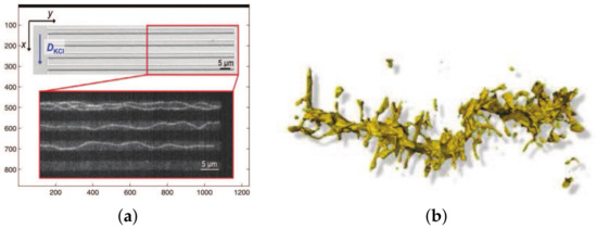
Figure 1. (a) Optical micrograph of a segment of the microfluidics comb-like structures (on top). On the bottom: microfluidic micrographs of fluorescently labeled, polymerized actin filaments in a comb-like structure [4]. (b) One of the examples of a physical environment suitable for the comb model. Electron tomogram of a spiny dendrite. Image taken from Internet (http://www.cacr.caltech.edu/projects/ldviz/results/levelsets/, accessed on 1 July 2013).

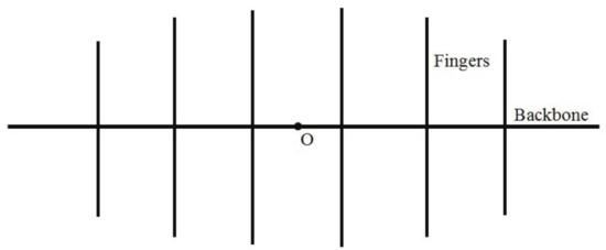
Figure 2. The schematic of a comb model.

Due to the geometrical structure and the non-uniformity of the medium transmission, the classical Fick’s law in conventional diffusion with the paradox of an infinite transport velocity [10,11] is no longer applicable. In order to study the transmission mechanism of the concentration field for the anomalous diffusion in the comb model, three modifications for the Fick’s model are presented. The first is the introduction of the relaxation parameter $\xi$ and the second considers the time-fractional derivatives with the motivation that the relaxation parameter makes the transport process attach a finite transport velocity, while the time-fractional derivative takes the memory characteristic of the transport process into account. Furthermore, as discussed in [12], due to the special structure of the comb model, the highly inhomogeneous characteristic happens along the x-axis, and this characteristic can be reflected by the space-fractional derivative [13]. Thus, as the third modification, the second space-integer derivative is modified to a space-fractional derivative with variable coefficients, which considers a left and right nonlocal characteristic. Based on the time-fractional Cattaneo model [14] and the two-dimensional space-fractional constitutive model [15], the following time- and space-fractional Cattaneo constitution relationship with variable diffusion coefficients is formulated

$$\begin{array}{c}\overrightarrow{J}(x,y,t)+\xi \frac{\partial \overrightarrow{J}(x,y,t)}{\partial t}\hfill \\ {=}_0^{RL}{D}_t^{1-\alpha }(-\delta \left(y\right)\left(d^{+}(x,y){}_L{D}_x^{\gamma }u(x,y,t)-d^{-}(x,y){}_x{D}_R^{\gamma }u(x,y,t)\right),-e(x,y)\frac{\partial u(x,y,t)}{\partial y}),\hfill \end{array}$$

(2)

where $\delta \left(y\right)d^{+}(x,y)$ and $\delta \left(y\right)d^{-}(x,y)$ represent the left and right variable diffusion coefficient along the x-direction, respectively; $e(x,y)$ refers to the variable diffusion coefficient along the y-direction; ${}_0^{RL}{D}_t^{1-\alpha }$ refers to time-fractional derivative of order $1-\alpha$ ($0<\alpha <1$) with the Riemann–Liouville definition; ${}_L{D}_x^{\gamma }$ and ${}_x{D}_R^{\gamma }$, respectively, denote the left and right Riemann–Liouville space-fractional derivatives of order $\gamma$ ($0<\gamma <1$). The definitions are, respectively, given by

$$\begin{array}{cc}\hfill {}_0^{RL}{D}_t^{1-\alpha }u(x,y,t)& =\frac{1}{\mathrm{\Gamma }\left(\alpha \right)}\frac{\partial }{\partial t}{\int }_0^t\frac{1}{{(t-\tau )}^{1-\alpha }}u\left(x,y,\tau \right)d\tau ,\hfill \\ \hfill {}_L{D}_x^{\gamma }u(x,y,t)=& \frac{1}{\mathrm{\Gamma }(1-\gamma )}\frac{\partial }{\partial x}{\int }_L^x\frac{1}{{(x-s)}^{\gamma }}u\left(s,y,t\right)ds,\hfill \\ \hfill {}_x{D}_R^{\gamma }u(x,y,t)=& \frac{-1}{\mathrm{\Gamma }\left(1-\gamma \right)}\frac{\partial }{\partial x}{\int }_x^R\frac{1}{{(s-x)}^{\gamma }}u(s,y,t)ds,\hfill \end{array}$$

where the symbol $\mathrm{\Gamma }(·)$ refers to the Euler gamma function, L and R refer to the left and right boundaries along the x-direction.

By combining the constitutive relation (2) with the following mass conservation equation

$$\begin{array}{c}\hfill \frac{\partial u(x,y,t)}{\partial t}+\nabla ·\overrightarrow{J}(x,y,t)=0,\end{array}$$

(3)

we obtain the time- and space-fractional Cattaneo governing equation

$$\begin{array}{cc}\hfill & \xi \frac{{\partial }^{1+\alpha }u(x,y,t)}{\partial t^{1+\alpha }}+\frac{{\partial }^{\alpha }u\left(x,y,t\right)}{\partial t^{\alpha }}\hfill \\ \hfill =& \frac{\partial }{\partial x}\left[\delta \left(y\right)(d^{+}\left(x,y\right){}_L{D}_x^{\gamma }u(x,y,t)-d^{-}\left(x,y\right){}_x{D}_R^{\gamma }u(x,y,t)\right)]+\frac{\partial }{\partial y}\left[e(x,y)\frac{\partial u\left(x,y,t\right)}{\partial y}\right],\hfill \end{array}$$

(4)

where the symbols $\frac{{\partial }^{\alpha }u\left(x,y,t\right)}{\partial t^{\alpha }}d\alpha$ and $\frac{{\partial }^{1+\alpha }u(x,y,t)}{\partial t^{1+\alpha }}$ denote the Caputo fractional derivative operators of order $\alpha$ and $1+\alpha$, respectively, in which the definitions are given as

$$\begin{array}{c}\frac{{\partial }^{\alpha }u\left(x,y,t\right)}{\partial t^{\alpha }}=\frac{1}{\mathrm{\Gamma }(1-\alpha )}{\int }_0^t\frac{1}{{(t-\tau )}^{\alpha }}\frac{\partial u(x,y,\tau )}{\partial \tau }d\tau ,\\ \frac{{\partial }^{1+\alpha }u\left(x,y,t\right)}{\partial t^{1+\alpha }}=\frac{1}{\mathrm{\Gamma }(1-\alpha )}{\int }_0^t\frac{1}{{(t-\tau )}^{\alpha }}\frac{{\partial }^{2}u(x,y,\tau )}{\partial {\tau }^2}d\tau .\end{array}$$

As a generalization of the integer derivative, the fractional operator considers the memory and nonlocal characteristics and has important applications in a variety of fields. For the fractional governing Equation (4), a limitation is that it is suitable for describing the probability density distribution of a very narrow class of diffusion processes because it is characterized by a unique time-fractional exponent [16]. Motivated by this idea, by integrating the fractional-order derivatives with respect to the order of differentiation, a distribution-order operator was proposed by Caputo [17]. The governing equation with the distributed-order operator exhibits memory and nonlocal effects over various time-fractional scales and becomes a powerful tool to describe transport phenomena in complex heterogeneous media. However, as far as we are aware, the distributed-order time and space diffusion-wave equation has not been considered to study the anomalous diffusion in the comb model.

Motivated by the above discussions, as an original contribution to the literature, we discuss and analyze the following distributed-order time- and space-fractional diffusion-wave equation to study the anomalous diffusion in the comb model

$$\begin{array}{c}\xi {\int }_1^2{\phi }_1\left(\beta \right)\frac{{\partial }^{\beta }u(x,y,t)}{\partial t^{\beta }}d\beta +{\int }_0^1{\phi }_0\left(\alpha \right)\frac{{\partial }^{\alpha }u\left(x,y,t\right)}{\partial t^{\alpha }}d\alpha \hfill \\ =\frac{\partial }{\partial x}\left[\delta \left(y\right)(d^{+}\left(x,y\right){}_L{D}_x^{\gamma }u(x,y,t)-d^{-}\left(x,y\right){}_x{D}_R^{\gamma }u(x,y,t)\right)]+\frac{\partial }{\partial y}\left[e(x,y)\frac{\partial u(x,y,t)}{\partial y}\right]+f\left(x,y,t\right),\hfill \end{array}$$

(5)

where ${\phi }_1\left(\beta \right)$ and ${\phi }_0\left(\alpha \right)$ denote weight functions and $\beta \in \left(1,2\right)$, ${\phi }_1\left(\beta \right)\ge 0$, ${\phi }_1\left(\beta \right)\not\equiv 0$, $0<{\int }_1^2{\phi }_1\left(\beta \right)d\beta <\infty$, $\alpha \in \left(0,1\right)$, ${\phi }_0\left(\alpha \right)\ge 0$, ${\phi }_0\left(\alpha \right)\not\equiv 0$, $0<{\int }_0^1{\phi }_0\left(\alpha \right)d\alpha <\infty$ and $f(x,y,t)$ is a source term.

As Ref. [6] indicated, the diffusion in the comb model, which is described by the Fick’s model, is an example of a subdiffusive one-dimensional medium where a continuous-time random walk takes place along the backbone while the diffusion along the y direction has a traps effect. The classical Fick’s model possesses the local characteristic, and the fractional derivative is proposed, considering the memory and nonlocal characteristics. For a further development, the distributed-order time-fractional derivative is proposed by integrating the fractional-order derivatives. In conclusion, Equation (5) is a development to describe the continuous-time random walk, considering various memory and nonlocal characteristics.

The anomalous diffusion in the comb model has been applied to many different fields in medicine and biology. In some applications of the comb model treating with the numerical method, the infinite regions are approximated by the rectangular domains with large sides [18]. However, by extending the computational modeling to irregular domains, we can broaden the potential applicability of the comb model. Based on these discussions, in this paper, the initial and boundary conditions are given by

$$\begin{array}{c}u(x,y,0)={\varphi }_0(x,y),u_t(x,y,0)={\varphi }_1(x,y),(x,y)\in \overline{\mathrm{\Omega }},\end{array}$$

(6)

$$\begin{array}{c}u(x,y,t)=0,(x,y,t)\in \partial \mathrm{\Omega }\times (0,T],\end{array}$$

(7)

respectively, where $\mathrm{\Omega }$ is an irregular convex domain.

The new governing Equation (5) is a generalization and development of the classical model to study the anomalous diffusion in the comb model. By choosing ${\phi }_0\left(\alpha \right)=\delta \left(\alpha -{\alpha }_0\right)$, ${\phi }_1\left(\beta \right)=\delta \left(\beta -{\alpha }_0-1\right)$, $d^{+}(x,y)=d^{-}(x,y)=k_x$, $e(x,y)=k_y$, $\gamma =1$ and $f(x,y,t)=0$, Equation (5) reduces to the time-fractional Cattaneo governing equation [14]

$$\xi \frac{{\partial }^{{\alpha }_0+1}u(x,y,t)}{\partial t^{{\alpha }_0+1}}+\frac{{\partial }^{{\alpha }_0}u(x,y,t)}{\partial t^{{\alpha }_0}}=k_x\delta \left(y\right)\frac{{\partial }^{2}u(x,y,t)}{\partial x^2}+k_y\frac{{\partial }^{2}u\left(x,y,t\right)}{\partial y^2}.$$

For the choice ${\phi }_0\left(\alpha \right)=\delta \left(\alpha -{\alpha }_0\right)$, $\xi =0$, $d^{+}\left(x,y\right)=k_x$, $d^{-}\left(x,y\right)=0$, $e(x,y)=k_y$ and $f(x,y,t)=0$, Equation (5) reduces to the time- and space-fractional governing equation [19]

$$\frac{{\partial }^{{\alpha }_0}u\left(x,y,t\right)}{\partial t^{{\alpha }_0}}=k_x\delta \left(y\right)\frac{{\partial }^{\gamma +1}u(x,y,t)}{\partial x^{\gamma +1}}+k_y\frac{{\partial }^{2}u(x,y,t)}{\partial y^2}.$$

Finally, by choosing $\xi =0$, ${\phi }_0\left(\alpha \right)=\delta \left(\alpha -1\right)$, $d^{+}\left(x,y\right)=d^{-}\left(x,y\right)=k_x$, $e(x,y)=k_y$, $\gamma =1$ and $f(x,y,t)=0$, we obtain the anomalous diffusion based on the classical Fick’s model [2]

$$\frac{\partial u\left(x,y,t\right)}{\partial t}=k_x\delta \left(y\right)\frac{{\partial }^{2}u\left(x,y,t\right)}{\partial x^2}+k_y\frac{{\partial }^{2}u(x,y,t)}{\partial y^2}.$$

The study of distributed-order time- and space-fractional diffusion-wave equations is of great significance to further improve and predict the anomalous diffusion phenomena in the comb-like structures.

2. The Structure of the Paper

In this paper, the two-dimensional irregular convex domain is defined as $\mathrm{\Omega }=\left\{(x,y)\right|x_L\left(y\right)\le x\le x_R\left(y\right),y_D\left(x\right)\le y\le y_U\left(x\right)\}$, where $x_L\left(y\right)$, $x_R\left(y\right)$, $y_D\left(x\right)$, $y_U\left(x\right)$ are the left, right, lower and upper boundaries of $\mathrm{\Omega }$, respectively. Denote $x_{min}=\underset{\left(x,y\right)\in \mathrm{\Omega }}{min}{x}_L\left(y\right)$, $x_{max}=\underset{\left(x,y\right)\in \mathrm{\Omega }}{max}{x}_R\left(y\right)$, $y_{min}=\underset{(x,y)\in \mathrm{\Omega }}{min}{y}_D\left(x\right)$, $y_{max}=\underset{(x,y)\in \mathrm{\Omega }}{max}{y}_U\left(x\right)$. Then, the inner product is defined as

$$\begin{array}{cc}\hfill {(u,v)}_{\mathrm{\Omega }}& ={\int }_{y_{min}}^{y_{max}}{\int }_{x_L\left(y\right)}^{x_R\left(y\right)}u\left(x,y\right)v\left(x,y\right)dxdy={\int }_{x_{min}}^{x_{max}}{\int }_{y_D\left(x\right)}^{y_U\left(x\right)}u\left(x,y\right)v\left(x,y\right)dxdy,\hfill \end{array}$$

and the $L^2$-norm is given as ${\Vert u\Vert }_{L^2\left(\mathrm{\Omega }\right)}={\left({(u,u)}_{\mathrm{\Omega }}\right)}^{1/2}.$

The fractional derivative space in one dimension was firstly established by Roop and Ervin [20] and then developed further by Bu et al. [21,22], Yang et al. [23], Hao et al. [24] and Wang et al. [25,26]. Due to the special form of the governing equation with a space-fractional derivative of order $\gamma$ in x and the integer derivative in y, some new definitions and lemmas of the fractional derivative spaces are defined.

Definition 1.

The definitions for the left (right) fractional derivative space with semi-norm and norm are, respectively, given as

$$\begin{array}{cc}\hfill & {\left|u\right|}_{J_L^{\gamma ,1}\left(\mathrm{\Omega }\right)}={\left(\Vert {}_L{D}_x^{\gamma }u{\Vert }_{L^2\left(\mathrm{\Omega }\right)}^2+\Vert \frac{\partial u}{\partial y}|{|}_{L^2\left(\mathrm{\Omega }\right)}^2\right)}^{1/2},{\left|u\right|}_{J_R^{\gamma ,1}\left(\mathrm{\Omega }\right)}={\left(\Vert {}_x{D}_R^{\gamma }u{\Vert }_{L^2\left(\mathrm{\Omega }\right)}^2+\Vert \frac{\partial u}{\partial y}|{|}_{L^2\left(\mathrm{\Omega }\right)}^2\right)}^{1/2},\hfill \\ \hfill & {\Vert u\Vert }_{J_L^{\gamma ,1}\left(\mathrm{\Omega }\right)}={\left({\Vert u\Vert }_{L^2\left(\mathrm{\Omega }\right)}^2+{\left|u\right|}_{J_L^{\gamma ,1}\left(\mathrm{\Omega }\right)}^2\right)}^{1/2}{,\Vert u\Vert }_{J_R^{\gamma ,1}\left(\mathrm{\Omega }\right)}={\left({\Vert u\Vert }_{L^2\left(\mathrm{\Omega }\right)}^2+{\left|u\right|}_{J_R^{\gamma ,1}\left(\mathrm{\Omega }\right)}^2\right)}^{1/2},\hfill \end{array}$$

where $J_L^{\gamma ,1}\left(\mathrm{\Omega }\right)$$\left(J_R^{\gamma ,1}\left(\mathrm{\Omega }\right)\right)$ denotes the closure of $C^{\infty }\left(\mathrm{\Omega }\right)$ with respect to $\Vert ·{\Vert }_{J_L^{\gamma ,1}\left(\mathrm{\Omega }\right)}$$\left(\Vert ·{\Vert }_{J_R^{\gamma ,1}\left(\mathrm{\Omega }\right)}\right)$.

Definition 2.

The fractional Sobolev space with the semi-norm and norm of order μ are, respectively, defined as

$$\begin{array}{cc}\hfill {\left|u\right|}_{H^{\mu }\left(\mathrm{\Omega }\right)}& =\Vert {\left|\xi \right|}^{\mu }\mathcal{F}\left(\widehat{u}\right)\left(\xi \right){\Vert }_{L^2\left({\mathbb{R}}^2\right)},\hfill \\ \hfill {\Vert u\Vert }_{H^{\mu }\left(\mathrm{\Omega }\right)}& ={\left({\Vert u\Vert }_{L^2\left(\mathrm{\Omega }\right)}^2+{\left|u\right|}_{H^{\mu }\left(\mathrm{\Omega }\right)}^2\right)}^{1/2},\hfill \end{array}$$

where $\mathcal{F}\left(\widehat{u}\right)\left(\xi \right)$ is the Fourier transformation of the function $\widehat{u}$, and $\widehat{u}$ is the zero extension of the function u outside of Ω, $H^{\mu }\left(\mathrm{\Omega }\right)$ denotes the closure of $C^{\infty }\left(\mathrm{\Omega }\right)$ with respect to $\Vert ·{\Vert }_{H^{\mu }\left(\mathrm{\Omega }\right)}$.

Definition 3.

For the symmetric fractional derivative space, when $\gamma \ne 1/2$, we define the semi-norm and norm

$$\begin{array}{cc}\hfill {\left|u\right|}_{J_S^{\gamma ,1}\left(\mathrm{\Omega }\right)}=& {\left(|{\left({}_L{D}_x^{\gamma }u,{}_x{D}_R^{\gamma }u\right)}_{\mathrm{\Omega }}|+\left|{\left(\frac{\partial u}{\partial y},\frac{\partial u}{\partial y}\right)}_{\mathrm{\Omega }}\right|\right)}^{1/2},\hfill \\ \hfill {\Vert u\Vert }_{J_S^{\gamma ,1}\left(\mathrm{\Omega }\right)}& ={\left({\Vert u\Vert }_{L^2\left(\mathrm{\Omega }\right)}^2+{\left|u\right|}_{J_S^{\gamma ,1}\left(\mathrm{\Omega }\right)}^2\right)}^{1/2},\hfill \end{array}$$

where $J_S^{\gamma ,1}\left(\mathrm{\Omega }\right)$ denotes the closure of $C^{\infty }\left(\mathrm{\Omega }\right)$ with respect to $\Vert ·{\Vert }_{J_S^{\gamma ,1}\left(\mathrm{\Omega }\right)}$.

We denote $J_{L,0}^{\gamma ,1}\left(\mathrm{\Omega }\right)$, $J_{R,0}^{\gamma ,1}\left(\mathrm{\Omega }\right)$, $H_0^{\gamma }\left(\mathrm{\Omega }\right)$, $H_0^1\left(\mathrm{\Omega }\right)$ and $J_{S,0}^{\gamma ,1}\left(\mathrm{\Omega }\right)$ as the closure of $C_0^{\infty }\left(\mathrm{\Omega }\right)$ with respect to $\Vert ·{\Vert }_{J_L^{\gamma ,1}\left(\mathrm{\Omega }\right)}$, $\Vert ·{\Vert }_{J_R^{\gamma ,1}\left(\mathrm{\Omega }\right)}$, $\Vert ·{\Vert }_{H^{\gamma }\left(\mathrm{\Omega }\right)}$, $\Vert ·{\Vert }_{H^1\left(\mathrm{\Omega }\right)}$ and $\Vert ·{\Vert }_{J_S^{\gamma ,1}\left(\mathrm{\Omega }\right)}$, respectively, where $C_0^{\infty }\left(\mathrm{\Omega }\right)$ is the space of smooth functions with compact support in $\mathrm{\Omega }$. Based on the above definitions, some useful and important lemmas are introduced.

Lemma 1.

For $u(x,y),v(x,y)\in J_{L,0}^{\gamma ,1}\left(\mathrm{\Omega }\right)\bigcap J_{R,0}^{\gamma ,1}\left(\mathrm{\Omega }\right)$$(0<\gamma <1)$, we have

$$\begin{array}{c}\hfill \left({}_L{D}_x^{\gamma }u\left(x,y\right),\frac{\partial v\left(x,y\right)}{\partial x}\right)=-\left({}_L{D}_x^{\left(\gamma +1\right)/2}u\left(x,y\right),{}_x{D}_R^{\left(\gamma +1\right)/2}v(x,y)\right),\end{array}$$

(8)

$$\begin{array}{c}\hfill \left({}_x{D}_R^{\gamma }u\left(x,y\right),\frac{\partial v\left(x,y\right)}{\partial x}\right)=-\left({}_x{D}_R^{\left(\gamma +1\right)/2}u\left(x,y\right),{}_L{D}_x^{\left(\gamma +1\right)/2}v(x,y)\right).\end{array}$$

(9)

Proof. 

See [27].    □

Lemma 2.

For $u\in H_0^{\gamma }\left(\mathrm{\Omega }\right)$ and $0<\gamma <(\gamma +1)/2$, then

$$\begin{array}{c}\hfill {\Vert u\Vert }_{L^2\left(\mathrm{\Omega }\right)}\le C_2\Vert {}_L{D}_x^{\gamma }u{\Vert }_{L^2\left(\mathrm{\Omega }\right)}\le C_1\Vert {}_L{D}_x^{\left(\gamma +1\right)/2}u{\Vert }_{L^2\left(\mathrm{\Omega }\right)},\end{array}$$

(10)

$$\begin{array}{c}\hfill {\Vert u\Vert }_{L^2\left(\mathrm{\Omega }\right)}\le C_4\Vert {}_x{D}_R^{\gamma }u{\Vert }_{L^2\left(\mathrm{\Omega }\right)}\le C_3\Vert {}_x{D}_R^{\left(\gamma +1\right)/2}u{\Vert }_{L^2\left(\mathrm{\Omega }\right)}.\end{array}$$

(11)

For $u\in H_0^1\left(\mathrm{\Omega }\right)$, we have

$$\begin{array}{c}\hfill {\Vert u\Vert }_{L^2\left(\mathrm{\Omega }\right)}\le C_5\Vert \frac{\partial u}{\partial y}|{|}_{L^2\left(\mathrm{\Omega }\right)},\end{array}$$

(12)

where $C_1$, $C_2$, $C_3$, $C_4$ and $C_5$ are positive constants independent of u.

Proof. 

The proof of this Lemma follows that given in [28].    □

Lemma 3.

For $u\left(x,y\right)\in J_{L,0}^{\gamma ,1}\left(\mathrm{\Omega }\right)\cap J_{R,0}^{\gamma ,1}\left(\mathrm{\Omega }\right)$, we have

$$\begin{array}{cc}\hfill \left({}_L{D}_x^{\left(\gamma +1\right)/2}u,{}_x{D}_R^{\left(\gamma +1\right)/2}u\right)& =cos\left(\pi \left(\gamma +1\right)/2\right)\Vert {}_L{D}_x^{\left(\gamma +1\right)/2}\widehat{u}|{|}_{L^2\left({\mathbb{R}}^2\right)}^2,\hfill \end{array}$$

(13)

$$\begin{array}{cc}\hfill \left(\frac{\partial u}{\partial y},\frac{\partial u}{\partial y}\right)& =\Vert \frac{\partial u}{\partial y}|{|}_{L^2\left({\mathbb{R}}^2\right)}^2.\hfill \end{array}$$

(14)

Proof. 

Similar to the derivation process in [27], we can obtain the results immediately.    □

Lemma 4.

If $u>0$, $\gamma \ne n-1/2$, $n\in \mathbb{N}$, then $J_{L,0}^{\gamma ,1}\left(\mathrm{\Omega }\right)$, $J_{R,0}^{\gamma ,1}\left(\mathrm{\Omega }\right)$, $J_{S,0}^{\gamma ,1}\left(\mathrm{\Omega }\right)$, $H_0^{\gamma }\left(\mathrm{\Omega }\right)$ and $H_0^1\left(\mathrm{\Omega }\right)$ are equivalent with equivalent norms and semi-norms.

Proof. 

The proof of this lemma can be found in [28].    □

3. Derivation of the Finite Element Scheme for the Comb Model

3.1. Finite Element Fully Variational Formulation

In the following section, for the sake of simplicity, denote $d_1(x,y)=\delta \left(y\right)d^{+}\left(x,y\right)$, $d_2(x,y)=\delta \left(y\right)d^{-}\left(x,y\right)$. Due to the irregular shape of the solution domain, the traditional rectangular mesh cannot be used. The finite element method is applied to obtain the solution of the governing Equation (5), subject to the initial conditions (6) and irregular boundary conditions (7).

Firstly, in the governing Equation (5), the distributed-order time-fractional derivatives are discretized using the mid-point quadrature rule [29]

$$\begin{array}{cc}\hfill {\int }_1^2{\phi }_1\left(\beta \right)\frac{{\partial }^{\beta }}{\partial t^{\beta }}\left(\frac{{\partial }^{2}u}{\partial x^2}\right)d\beta & =\sum _{i=0}^{M_1}{\omega }_i^{\left(1\right)}\frac{{\partial }^{{\beta }_i}}{\partial t^{{\beta }_i}}\left(\frac{{\partial }^{2}u}{\partial x^2}\right)+O\left(h_{\beta }^2\right),\hfill \\ \hfill {\int }_0^1{\phi }_0\left(\alpha \right)\frac{{\partial }^{\alpha +1}}{\partial t^{\alpha +1}}d\alpha & =\sum _{i=0}^{M_2}{\omega }_i^{\left(2\right)}\frac{{\partial }^{{\alpha }_i+1}u}{\partial t^{{\alpha }_i+1}}+O\left(h_{\alpha }^2\right),\hfill \end{array}$$

where ${\omega }_i^{\left(1\right)}=h_{\beta }{\phi }_1\left({\alpha }_i\right)$, ${\omega }_i^{\left(2\right)}=h_{\alpha }{\phi }_0\left({\alpha }_i\right)$, $h_{\alpha }=\frac{1}{M_2+1}$ and $h_{\beta }=\frac{1}{M_1+1}$ are fractional parameter steps and ${\alpha }_i=\frac{i{h}_{\alpha }+(i+1)h_{\alpha }}{2}$ for $i=0,1,\dots ,M_2$, ${\beta }_i=\frac{i{h}_{\beta }+(i+1)h_{\beta }}{2}$ for $i=0,1,\dots ,M_1$.

Let $\tau =T/N$ be the time step and $t_k=k\tau$ ($k=0,1,\dots ,N$) where N is a positive integer. Denote $u^{k-1/2}=\frac{u^k+u^{k-1}}{2}$ for $k=1,\dots ,N$. For $u(x,y,t)\in C(\mathrm{\Omega }\times [0,T\left]\right)$, denote $u^k=u^k(·)=u(·,t_k)$. We introduce ${\nabla }_t{u}^{k-1/2}=\frac{u^k-u^{k-1}}{\tau }$. At $t=t_{k-1/2}$, the L2-scheme [30] to approximate the fractional derivative of order ${\beta }_i$ ($1<{\beta }_i<2$) with the Caputo definition is given as

$$\begin{array}{cc}\hfill \frac{{\partial }^{{\beta }_i}{u}^{k-1/2}}{\partial t^{{\beta }_i}}=& \frac{{\tau }^{1-{\beta }_i}}{\mathrm{\Gamma }\left(3-{\beta }_i\right)}\left[a_0^{\left({\beta }_i\right)}{\nabla }_t{u}^{k-1/2}-\sum _{j=1}^{k-1}\left(a_{k-1-j}^{\left({\beta }_i\right)}-a_{k-j}^{\left({\beta }_i\right)}\right){\nabla }_t{u}^{j-1/2}-a_{k-1}^{\left({\beta }_i\right)}{u}_t^0\right]+R_0^{k,{\beta }_i}\hfill \\ \hfill =& {\nabla }_t^{\left({\beta }_i\right)}{u}^{k-1/2}+R_0^{k,{\beta }_i},\hfill \end{array}$$

(15)

where $a_j^{\left({\beta }_i\right)}={\left(j+1\right)}^{2-{\beta }_i}-j^{2-{\beta }_i}$, $j=0,1,2,\dots ,k-1$, $|R_0^{k,{\beta }_i}|\le C\left({\tau }^{3-{\beta }_i}\right)$.

Lemma 5.

For the above $a_j^{\left({\beta }_i\right)}$, define vector $S={\left[S_1,S_2,S_3,\dots ,S_N\right]}^T$ and constant P, it holds that

$$\begin{array}{c}\hfill \frac{2{\tau }^{1-{\beta }_i}}{\mathrm{\Gamma }\left(3-{\beta }_i\right)}\sum _{k=1}^N\left[a_0^{\left({\beta }_i\right)}{S}_k-\sum _{j=1}^{k-1}\left(a_{k-j-1}^{\left({\beta }_i\right)}-a_{k-j}^{\left({\beta }_i\right)}\right)S_j-a_{k-1}^{\left({\beta }_i\right)}P\right]S_k\ge \frac{T^{1-{\beta }_i}}{\mathrm{\Gamma }\left(2-{\beta }_i\right)}\sum _{k=1}^N{S}_k^2-\frac{T^{2-{\beta }_i}}{\tau \mathrm{\Gamma }\left(3-{\beta }_i\right)}{P}^2.\end{array}$$

Proof. 

See [30].    □

The time Caputo fractional derivative of order ${\alpha }_i$ ($0<{\alpha }_i<1$) is discretized by using the L1-scheme [30], and the scheme at $t=t_{k-1/2}$ is given as

$$\begin{array}{cc}\hfill \frac{{\partial }^{{\alpha }_i}{u}^{k-1/2}}{\partial t^{{\alpha }_i}}=& \frac{{\tau }^{1-{\alpha }_i}}{2\mathrm{\Gamma }\left(2-{\alpha }_i\right)}\sum _{j=1}^k{b}_{k-j}^{\left({\alpha }_i\right)}{\nabla }_t{u}^{j-1/2}+\frac{{\tau }^{1-{\alpha }_i}}{2\mathrm{\Gamma }\left(2-{\alpha }_i\right)}\sum _{j=1}^{k-1}{b}_{k-j-1}^{\left({\alpha }_i\right)}{\nabla }_t{u}^{j-1/2}+R_1^{k,{\alpha }_i}\hfill \\ \hfill =& {\nabla }_t^{\left({\alpha }_i\right)}{u}^{k-\frac{1}{2}}+R_1^{k,{\alpha }_i},\hfill \end{array}$$

(16)

where $b_j^{\left({\alpha }_i\right)}={\left(j+1\right)}^{1-{\alpha }_i}-j^{1-{\alpha }_i}$, $j=0,1,2,\dots ,k-1$, $|R_1^{k,{\alpha }_i}|\le C\left({\tau }^{2-{\alpha }_i}\right)$.

Lemma 6.

For the above $b_j^{\left({\alpha }_i\right)}$, choosing any positive integer M and vector $\left[v_1,v_2,v_3,\dots ,v_M\right]\in {\mathbb{R}}^M$, we have

$$\begin{array}{c}\hfill \sum _{k=1}^M\sum _{j=1}^k{b}_{k-j}^{\left({\alpha }_i\right)}\left(v_j,v_k\right)+\sum _{k=1}^M\sum _{j=1}^{k-1}{b}_{k-j-1}^{\left({\alpha }_i\right)}\left(v_j,v_k\right)\ge 0.\end{array}$$

Proof. 

See [31].    □

At time $t=t_{k-1/2}$, the semi-discrete scheme for the governing Equation (5) is given as follows:

$$\begin{array}{c}\xi \sum _{i=0}^{M_1}{\omega }_i^{\left(1\right)}{\nabla }_t^{\left({\beta }_i\right)}{u}^{k-1/2}+\frac{1}{2}\sum _{i=0}^{M_2}{\omega }_i^{\left(2\right)}{\nabla }_t^{\left({\alpha }_i\right)}{u}^{k-1/2}\hfill \\ \hfill =\frac{\partial }{\partial x}\left[d_1\left(x,y\right){}_L{D}_x^{\gamma }{u}^{k-1/2}-d_2\left(x,y\right){}_x{D}_R^{\gamma }{u}^{k-1/2}\right]+e\left(x,y\right)\frac{{\partial }^2{u}^{k-1/2}}{\partial y^2}+f^{k-1/2}.\end{array}$$

(17)

Define $V=H_0^{\gamma }\left(\mathrm{\Omega }\right)\cap H_0^1\left(\mathrm{\Omega }\right)$ to be the numerical solution space. In this work, we choose to use triangular elements to mesh $\mathrm{\Omega }$. Because the domain is irregularly shaped, we refer to this throughout this paper as an unstructured mesh. Denote $\left\{{\mathrm{\Gamma }}_h\right\}$ as a family of unstructured triangulations of domain $\mathrm{\Omega }$, where h is the maximum diameter of any triangle in ${\mathrm{\Gamma }}_h$. Then, we obtain the conforming finite element subspace $V_h\in V$ as

$$\begin{array}{c}\hfill V_h=\left\{v_h\right|v_h\in C\left(\overline{\mathrm{\Omega }}\right)\cap V,v_h|{}_K\mathrm{is}\mathrm{linear}\mathrm{for}\mathrm{all}K\in {\mathrm{\Gamma }}_h\mathrm{and}{v}_h{|}_{\partial \mathrm{\Omega }}=0\}.\end{array}$$

Assume that $u_h^k$ is the approximation of $u(x,y,t)$ at time $t=t_k$. We can derive the fully discrete formulation of (5)–(7): find $u_h^k\in V_h$, for any $k=0,1,\dots ,N$, such that

$$\begin{array}{cc}\hfill \xi \sum _{i=0}^{M_1}& \frac{{\omega }_i^{\left(1\right)}{\tau }^{1-{\beta }_i}}{\mathrm{\Gamma }\left(3-{\beta }_i\right)}\left[a_0^{{\beta }_i}\left({\nabla }_t{u}_h^{k-1/2},v_h\right)-\sum _{j=1}^{k-1}\left(a_{k-1-j}^{\left({\beta }_i\right)}-a_{k-j}^{\left({\beta }_i\right)}\right)\left({\nabla }_t{u}_h^{j-1/2},v_h\right)-a_{k-1}^{\left({\beta }_i\right)}\left({\left(u_h^0\right)}_t,v_h\right)\right]\hfill \\ \hfill +& \frac{1}{2}\sum _{i=0}^{M_2}\frac{{\omega }_i^{\left(2\right)}{\tau }^{1-{\alpha }_i}}{\mathrm{\Gamma }\left(2-{\alpha }_i\right)}\sum _{j=1}^k{b}_{k-j}^{\left({\alpha }_i\right)}\left({\nabla }_t{u}_h^{j-1/2},v_h\right)+\frac{1}{2}\sum _{i=0}^{M_2}\frac{{\omega }_i^{\left(2\right)}{\tau }^{1-{\alpha }_i}}{\mathrm{\Gamma }\left(2-{\alpha }_i\right)}\sum _{j=1}^{k-1}{b}_{k-j-1}^{\left({\alpha }_i\right)}\left({\nabla }_t{u}_h^{j-1/2},v_h\right)\hfill \\ \hfill =& -B\left(u_h^{k-1/2},v_h\right)+\left(f^{k-1/2},v_h\right),\hfill \end{array}$$

(18)

with the initial conditions and boundary conditions given by

$$\begin{array}{c}\hfill u_h^0=u_{0h},u_h^k{|}_{\left(\partial \mathrm{\Omega }\right)}=0,\end{array}$$

(19)

where $u_{0h}\in V_h$ is a reasonable approximation for $u^0$. The expression for $B(u,v)$ is given as

$$\begin{array}{c}\hfill B\left(u,v\right)=\left(d_1\left(x,y\right){}_L{D}_x^{\gamma }u,\frac{\partial v}{\partial x}\right)-\left(d_2\left(x,y\right){}_x{D}_R^{\gamma }u,\frac{\partial v}{\partial x}\right)+\left(e\left(x,y\right)\frac{\partial u}{\partial y},\frac{\partial v}{\partial y}\right).\end{array}$$

(20)

3.2. Implementation of Finite Element Method with an Unstructured Mesh

In this section, we provide details of the implementation of the finite element method with an unstructured mesh. Firstly, we use the software Gmsh [32] to partition the convex domain $\mathrm{\Omega }$ with unstructured triangular elements. For every triangular element $e_p$, define $N_e$ as total number of the triangles and $N_P$ is the number of elements. Using piecewise linear polynomials on every triangular element $e_p$, for each time step, we can write $u_h^k$ in the form $u_h^k={\displaystyle \sum _{n=1}^{N_P}}{u}_n^k{\phi }_n(x,y)$, where ${\phi }_n(x,y)$ is the basis function and $u_n^k$ is the unknown to be solved for. Denote ${\phi }_n\left(x_m,y_m\right)={\delta }_{nm}$$(n,m=1,2,\dots ,N_p)$, where ${\delta }_{nm}$ refers to the Kronecker delta function, $v_h={\phi }_m\left(x,y\right)$, the mass matrix $M={\left({\phi }_n,{\phi }_m\right)}_{N_p\times N_p}$, the stiffness matrix $A={B\left({\phi }_n,{\phi }_m\right)}_{N_p\times N_p}$, $F^k={\left(F_1^k,F_2^k,\dots ,F_{N_p}^k\right)}^T$ where $F_m^k=\left(\frac{f^k+f^{k-1}}{2},{\phi }_m\right)$, ${\omega }_m^0=({\left(u_h^0\right)}_t$,${\phi }_m)$, $U^k={\left[u_1^k,u_2^k,\dots ,u_{N_p}^k\right]}^T$, $W^0={\left[{\omega }_1^0,{\omega }_2^0,\dots ,{\omega }_{N_p}^0\right]}^T$, then we can rewrite (18) in matrix forms as follows

$$\begin{array}{cc}\hfill & \left[\left(2\xi \sum _{i=0}^{M_1}{\omega }_i{a}_0^{\left({\beta }_i\right)}+2\sum _{i=0}^{M_2}{r}_i{b}_0^{\left({\alpha }_i\right)}\right)M+\tau A\right]U^k\hfill \\ \hfill =& \left[\left(2\xi \sum _{i=0}^{M_1}{\omega }_i{a}_0^{\left({\beta }_i\right)}+2\sum _{i=0}^{M_2}{r}_i{b}_0^{\left({\alpha }_i\right)}\right)M+\tau A\right]U^{k-1}+2\xi \tau \sum _{i=0}^{M_1}{\omega }_i{a}_{k-1}^{\left({\beta }_i\right)}{W}^0+2\tau F^k\hfill \\ \hfill +& 2\xi \sum _{i=0}^{M_1}{\omega }_i\sum _{j=1}^{k-1}\left(a_{k-1-j}^{\left({\beta }_i\right)}-a_{k-j}^{\left({\beta }_i\right)}\right)\left[M{U}^j-M{U}^{j-1}\right]-2\sum _{i=0}^{M_2}{r}_i\sum _{j=1}^{k-1}\left(b_{k-j}^{\left({\alpha }_i\right)}+b_{k-j-1}^{\left({\alpha }_i\right)}\right)\left[M{U}^j-M{U}^{j-1}\right],\hfill \end{array}$$

where ${\omega }_i=\frac{{\omega }_i^{\left(1\right)}{\tau }^{1-{\beta }_i}}{\mathrm{\Gamma }\left(3-{\beta }_i\right)}$, $r_i=\frac{{\omega }_i^{\left(2\right)}{\tau }^{1-{\alpha }_i}}{2\mathrm{\Gamma }\left(2-{\alpha }_i\right)}$.

The critical point to obtain the solution is to approximate the first and the second terms of $B\left({\phi }_n,{\phi }_m\right)$. By applying the Gauss quadrature [23], we obtain

$$\begin{array}{cc}\hfill \left(d_1\left(x,y\right){}_L{D}_x^{\gamma }{\phi }_n,\frac{\partial {\phi }_m}{\partial x}\right)=& \sum _{E\in {\mathrm{\Gamma }}_h}{\int }_E{d}_1\left(x,y\right){}_L{D}_x^{\gamma }{\phi }_n\frac{\partial {\phi }_m}{\partial x}dxdy\hfill \\ \hfill \approx & \sum _{E\in {\mathrm{\Gamma }}_h}\sum _{\left(x_{ci},y_{ci}\right)\in G_E}{\lambda }_i{d}_1\left(x,y\right){{}_L{D}_x^{\gamma }{\phi }_n|}_{\left(x_{ci},y_{ci}\right)}{\frac{\partial {\phi }_m}{\partial x}|}_{\left(x_{ci},y_{ci}\right)},\hfill \\ \hfill \left(d_2\left(x,y\right){}_R{D}_x^{\gamma }{\phi }_n,\frac{\partial {\phi }_m}{\partial x}\right)=& \sum _{E\in {\mathrm{\Gamma }}_h}{\int }_E{d}_2{\left(x,y\right)}_x{D}_R^{\gamma }{\phi }_n\frac{\partial {\phi }_m}{\partial x}dxdy\hfill \\ \hfill \approx & \sum _{E\in {\mathrm{\Gamma }}_h}\sum _{\left(x_{ci},y_{ci}\right)\in G_E}{\kappa }_i{d}_2\left(x,y\right){{}_x{D}_R^{\gamma }{\phi }_n|}_{\left(x_{ci},y_{ci}\right)}{\frac{\partial {\phi }_m}{\partial x}|}_{\left(x_{ci},y_{ci}\right)},\hfill \end{array}$$

where $G_E$ is the set of Gauss points in a certain element E and ${\lambda }_i$, ${\kappa }_i$ are the weight coefficients corresponding to the Gauss points $\left(x_{ci},y_{ci}\right)$. In this article, we used four Gauss points in each triangle.

Remark 1.

I would be precise on the number of Gauss points used and the accuracy of the approximation used.

In this paper, we use four Gauss points in every triangle.

The detailed computation process can be summarized in Algorithm 1.

Algorithm 1. Calculate $\left(d_1\left(x,y\right){}_L{D}_x^{\gamma }{\phi }_n,\frac{\partial {\phi }_m}{\partial x}\right)$ and $\left(d_2\left(x,y\right){}_R{D}_x^{\gamma }{\phi }_n,\frac{\partial {\phi }_m}{\partial x}\right)$ using finite element method on an unstructured mesh

1: By using the software Gmsh, partition the convex domain $\mathrm{\Omega }$ with unstructured triangular elements $e_p$ and save the information for node number $N_e$, coordinates $(x,y)$ and element number $N_P$; 2: for $p=1,2,\cdots ,N_e$ do 3:    For each triangle element $e_p$, find the Gauss points $(x_i,y_i)$ and corresponding weights ${\omega }_i$; 4:    for $j=1,2,\cdots ,N_p$ do 5:      Find the support domain ${\mathrm{\Omega }}_{e_j}$ and construct the support domain ${\mathrm{\Omega }}_{Lx}^n$ and ${\mathrm{\Omega }}_{xR}^n$; 6:      Use the line $y=y_i$ to insert ${\mathrm{\Omega }}_{e_j}$, find the intersection points and save the coordinates $(x_k,y_k)$; 7:      Apply piecewise linear polynomials on $e_p$ and calculate the piecewise continuous function ${\phi }_n(x,y_c)$; 8:      Calculate ${}_L{\tilde{D}}_x^{\alpha }{\phi }_n{|}_{(x_i,y_i)}$, ${}_x{\tilde{D}}_R^{\alpha }{\phi }_n{|}_{(x_i,y_i)}$. 9:    end for 10:    Calculate $\left(d_1\left(x,y\right){}_L{D}_x^{\gamma }{\phi }_n,\frac{\partial {\phi }_m}{\partial x}\right)$ and $\left(d_2\left(x,y\right){}_R{D}_x^{\gamma }{\phi }_n,\frac{\partial {\phi }_m}{\partial x}\right)$ 11: end for

4. Stability and Convergence

In this section, we analyze the stability and convergence of the discrete scheme on the irregular convex domain. In the following section, for the sake of simplicity, we consider the constant diffusion coefficient case $d_1(x,y)=d_2(x,y)=e(x,y)=1$. Denote $(·,·)={(·,·)}_{\mathrm{\Omega }}$, $\Vert ·{\Vert }_0=\Vert ·{\Vert }_{L^2\left(\mathrm{\Omega }\right)}$. Prior to presenting the numerical analysis, we firstly give the definitions of the semi-norm ${|·|}_{(\gamma ,1)}$ and norm $\Vert ·{\Vert }_{(\gamma ,1)}$

$$\begin{array}{cc}\hfill {\left|u\right|}_{(\gamma ,1)}& ={\left(\Vert {}_L{D}_x^{\left(\gamma +1\right)/2}u|{|}_0^2+\Vert \frac{\partial u}{\partial y}|{|}_0^2\right)}^{1/2},\hfill \end{array}$$

(21)

$$\begin{array}{cc}\hfill & {\Vert u\Vert }_{(\gamma ,1)}={\left({\Vert u\Vert }_0^2+{\left|u\right|}_{\left(\gamma ,1\right)}^2\right)}^{1/2}.\hfill \end{array}$$

(22)

In what follows, the constant C may be different in various sections.

4.1. Stability

Lemma 7.

For any $u\in V$, the semi-norm ${\left|u\right|}_{\left(\gamma ,1\right)}$ and norm ${\Vert u\Vert }_{\left(\gamma ,1\right)}$ are equivalent and there exists positive constants $C_1$ and $C_2$ independent of u, such that

$$\begin{array}{c}\hfill C_1{\Vert u\Vert }_{\left(\gamma ,1\right)}\le {\left|u\right|}_{\left(\gamma ,1\right)}\le {\Vert u\Vert }_{\left(\gamma ,1\right)}\le C_2{\left|u\right|}_{H^1\left(\mathrm{\Omega }\right)}.\end{array}$$

Proof. 

From Lemma 2, we immediately have

$$\begin{array}{c}\hfill {\Vert u\Vert }_0\le C\Vert {}_L{D}_x^{\left(\gamma +1\right)/2}u{\Vert }_0\le C{\left|u\right|}_{\left(\gamma ,1\right)}.\end{array}$$

By applying Lemma 2 and the Definitions (21) and (22), we have

$$\begin{array}{c}\hfill {\Vert u\Vert }_{\left(\gamma ,1\right)}=C_2{\left({\Vert u\Vert }_0^2+{\left|u\right|}_{\left(\gamma ,1\right)}^2\right)}^{1/2}\le C_2{\left|u\right|}_{\left(\gamma ,1\right)}\le C{\left|u\right|}_{J_L^{\gamma ,1}\left(\mathrm{\Omega }\right)}\le C_2{\left|u\right|}_{H^1\left(\mathrm{\Omega }\right)}.\end{array}$$

By using Lemma 4 and applying the definitions of the norm and semi-norm, we have

$$\begin{array}{c}\hfill {\Vert u\Vert }_{\left(\gamma ,1\right)}={\left({\Vert u\Vert }_0^2+{\left|u\right|}_{\left(\gamma ,1\right)}^2\right)}^{1/2}\ge {\left({\left|u\right|}_{\left(\gamma ,1\right)}^2\right)}^{1/2}={\left|u\right|}_{\left(\gamma ,1\right)}.\end{array}$$

(23)

The proof is completed. □

Lemma 8.

For any $u,v\in H_0^{\gamma }\left(\mathrm{\Omega }\right)\cap H_0^1\left(\mathrm{\Omega }\right)$, there exists constants $C_1$ and $C_2$ such that the function $B(u,v)$ satisfies $\left|B\left(u,v\right)\right|\le C_1{\Vert u\Vert }_{\left(\gamma ,1\right)}{\Vert v\Vert }_{\left(\gamma ,1\right)}$ and $B\left(u,u\right)\ge C_2{\Vert u\Vert }_{\left(\gamma ,1\right)}^2$.

Proof. 

Firstly, by using Lemma 1, Lemma 4 and Lemma 7, the Definitions (21) and (22) and applying the Cauchy–Schwartz inequality, namely $\left(u,v\right)\le {\Vert u\Vert }_0{\Vert v\Vert }_0$, we have

$$\begin{array}{cc}\hfill |B(u,v)|\le & \left[|\left({}_L{D}_x^{\left(\gamma +1\right)/2}u{,}_x{D}_R^{\left(\gamma +1\right)/2}v\right)|+|\left({}_x{D}_R^{\left(\gamma +1\right)/2}u{,}_L{D}_x^{\left(\gamma +1\right)/2}v\right)|+|\left(\frac{\partial u}{\partial y},\frac{\partial v}{\partial y}\right)|\right]\hfill \\ \hfill \le & \left[{\Vert {}_L{D}_x^{\left(\gamma +1\right)/2}u\Vert }_0{\Vert {}_x{D}_R^{\left(\gamma +1\right)/2}v\Vert }_0+{\Vert {}_x{D}_R^{\left(\gamma +1\right)/2}u\Vert }_0{\Vert {}_L{D}_x^{\left(\gamma +1\right)/2}v\Vert }_0+{\Vert \frac{\partial u}{\partial y}\Vert }_0{\Vert \frac{\partial v}{\partial y}\Vert }_0\right]\hfill \\ \hfill \le & C\left({\left|u\right|}_{\left(\gamma ,1\right)}{\left|v\right|}_{\left(\gamma ,1\right)}+{\left|u\right|}_{\left(\gamma ,1\right)}{\left|v\right|}_{\left(\gamma ,1\right)}+{\left|u\right|}_{\left(\gamma ,1\right)}{\left|v\right|}_{\left(\gamma ,1\right)}\right)\le C{\Vert u\Vert }_{\left(\gamma ,1\right)}{\Vert v\Vert }_{\left(\gamma ,1\right)},\hfill \\ \hfill B\left(u,u\right)& \ge \left[|\left({}_L{D}_x^{\left(\gamma +1\right)/2}u,{}_x{D}_R^{\left(\gamma +1\right)/2}u\right)|+|\left({}_x{D}_R^{\left(\gamma +1\right)/2}u,{}_L{D}_x^{\left(\gamma +1\right)/2}u\right)|+|\left(\frac{\partial u}{\partial y},\frac{\partial u}{\partial y}\right)|\right]\hfill \\ \hfill & \ge C\left[|\left({}_L{D}_x^{\left(\gamma +1\right)/2}u,{}_x{D}_R^{\left(\gamma +1\right)/2}u\right)|+|\left(\frac{\partial u}{\partial y},\frac{\partial u}{\partial y}\right)|\right]\ge {C|u|}_{H^1\left(\mathrm{\Omega }\right)}^2\ge {C\Vert u\Vert }_{\left(\gamma ,1\right)}^2.\hfill \end{array}$$

□

Theorem 1.

(Stability) The fully discrete scheme (18) is unconditionally stable and it holds that

$$\begin{array}{c}\hfill \Vert u_h^N{\Vert }_{\left(\gamma ,1\right)}\le C\left[\underset{1\le k\le N}{max}\Vert f^{k-1/2}{\Vert }_0^2+\Vert {\varphi }_1{\Vert }_1^2+{\Vert {\varphi }_0\Vert }_{\left(\gamma ,1\right)}\right].\end{array}$$

Proof. 

Denote $v_h={\nabla }_t{u}_h^{k-1/2}$. By multiplying $2\tau$ with each item and summing k from 1 to N, the discrete scheme (18) changes as

$$\begin{array}{cc}\hfill & 2\tau \xi \sum _{i=0}^{M_1}{\omega }_i^{\left(1\right)}\sum _{k=1}^N\left({\nabla }_t^{\left({\beta }_i\right)}{u}_h^{k-1/2},{\nabla }_t{u}_h^{k-1/2}\right)+2\tau \sum _{k=1}^N\sum _{i=0}^{M_2}{\omega }_i^{\left(2\right)}\left({\nabla }_t^{\left({\alpha }_i\right)}{u}_h^{k-1/2},{\nabla }_t{u}_h^{k-1/2}\right)\hfill \\ \hfill +& 2\tau \sum _{k=1}^{N}B\left(u_h^{k-1/2},{\nabla }_t{u}_h^{k-1/2}\right)-2\tau \sum _{k=1}^N\left(f^{k-1/2},{\nabla }_t{u}_h^{k-1/2}\right)=0.\hfill \end{array}$$

(24)

For the first term with the initial condition ${\left(u_h^0\right)}_t={\varphi }_1$, by using Lemma 5, we have

$$\begin{array}{c}\hfill 2\tau \xi \sum _{i=0}^{M_1}{\omega }_i^{\left(1\right)}\sum _{k=1}^N\left({\nabla }_t^{\left({\beta }_i\right)}{u}_h^{k-1/2},{\nabla }_t{u}_h^{k-1/2}\right)\ge 2\tau \xi a_1\sum _{k=1}^N\Vert {\nabla }_t{u}_h^{k-1/2}|{|}_0^2-\xi a_2\Vert {\varphi }_1{\Vert }_0^2,\end{array}$$

(25)

where $a_1={\displaystyle \sum _{i=0}^{M_1}}\frac{{\omega }_i^{\left(1\right)}{T}^{1-{\beta }_i}}{2\mathrm{\Gamma }\left(2-{\beta }_i\right)}$, $a_2={\displaystyle \sum _{i=0}^{M_1}}\frac{{\omega }_i^{\left(1\right)}{T}^{2-{\beta }_i}}{\mathrm{\Gamma }\left(3-{\beta }_i\right)}$.

By applying Lemma 6, we have

$$\begin{array}{c}\hfill 2\tau \sum _{k=1}^N\sum _{i=0}^{M_2}{\omega }_i^{\left(2\right)}\left({\nabla }_t^{\left({\alpha }_i\right)}{u}_h^{k-1/2},{\nabla }_t{u}_h^{k-1/2}\right)\ge 0.\end{array}$$

(26)

Define a symmetrical and continuous function

$$\begin{array}{c}\hfill B_0(u,v)=\left|\left({}_L{D}_x^{\left(\gamma +1\right)/2}u{,}_x{D}_R^{\left(\gamma +1\right)/2}v\right)\right|+\left|\left({}_x{D}_R^{\left(\gamma +1\right)/2}u{,}_L{D}_x^{\left(\gamma +1\right)/2}v\right)\right|+\left|\left(\frac{\partial u}{\partial y},\frac{\partial v}{\partial y}\right)\right|,\end{array}$$

(27)

then we have $B(u,v)\le C{B}_0(u,v)$. For the newly defined function $B_0\left(u_h^{k-1/2},{\nabla }_t{u}_h^{k-1/2}\right)$, we have $B_0\left(u_h^{k-1/2},{\nabla }_t{u}_h^{k-1/2}\right)=\frac{1}{2\tau }\left[B_0\left(u_h^k,u_h^k\right)-B_0\left(u_h^{k-1},u_h^{k-1}\right)\right]$ [21,22]. Perform the summation of k from 1 to N, and we derive the following inequality

$$\begin{array}{cc}\hfill & 2\tau \sum _{k=1}^{N}B\left(u_h^{k-1/2},{\nabla }_t{u}_h^{k-1/2}\right)\le 2\tau C\sum _{k=1}^N{B}_0\left(u_h^{k-1/2},{\nabla }_t{u}_h^{k-1/2}\right)\hfill \\ \hfill =& 2\tau C\sum _{k=1}^N\frac{1}{2\tau }\left[B\left(u_h^k,u_h^k\right)-B\left(u_h^{k-1},u_h^{k-1}\right)\right]=C\left(B\left(u_h^N,u_h^N\right)-B\left(u_h^0,u_h^0\right)\right).\hfill \end{array}$$

(28)

By using the important inequality $2ab\le \frac{a^2}{2\epsilon }+2\epsilon b^2$, the fifth item changes as

$$\begin{array}{cc}\hfill \sum _{k=1}^{N}2\tau \left(f^{k-1/2},{\nabla }_t{u}_h^{k-1/2}\right)& \le \sum _{k=1}^N\tau \left[\frac{\left|\right|f^{k-1/2}{\left|\right|}_0^2}{2a_1\xi }+2a_1\xi \Vert {\nabla }_t{u}_h^{k-1/2}|{|}_0^2\right]\hfill \\ \hfill & \le \frac{T}{2a_1\xi }\underset{1\le k\le N}{max}\Vert f^{k-1/2}{\Vert }_0^2+2a_1\xi \sum _{k=1}^N\tau \Vert {\nabla }_t{u}_h^{k-1/2}|{|}_0^2.\hfill \end{array}$$

(29)

Then, by using the inequality of (25)–(29), Equation (24) changes as

$$\begin{array}{c}\hfill B\left(u_h^N,u_h^N\right)\le C\left[\frac{T}{2a_1\xi }\underset{1\le k\le N}{max}\Vert f^{k-1/2}{\Vert }_0^2+a_2\xi \Vert {\varphi }_1{\Vert }_0^2+B\left(u_h^0,u_h^0\right)\right].\end{array}$$

Applying Lemma 8, we have

$$\begin{array}{c}\hfill \Vert u_h^N{\Vert }_{\left(\gamma ,1\right)}^2\le C\left[\underset{1\le k\le N}{max}\Vert f^{k-1/2}{\Vert }_0^2+\Vert {\varphi }_1{\Vert }_0^2+{\Vert {\varphi }_0\Vert }_{\left(\gamma ,1\right)}\right].\end{array}$$

Therefore, the scheme is unconditionally stable. □

4.2. Convergence

Prior to providing the convergence of the discrete scheme, we first give an approximation property. Define the interpolation operator $I_h$: $H^{s+1}\left(\mathrm{\Omega }\right)\to V_h$, for any $u\in H^{\mu }\left(\mathrm{\Omega }\right)$, $1<\mu \le s+1$, there exists a constant C depending only on $\mathrm{\Omega }$ such that [28]

$$\begin{array}{c}\hfill \Vert u-I_{h}u{\Vert }_{H^1\left(\mathrm{\Omega }\right)}\le C{h}^{\mu -1}{\Vert u\Vert }_{H^{\mu }\left(\mathrm{\Omega }\right)}.\end{array}$$

(30)

For any $u\in V$ and $v_h\in V_h$, we define a projection operator $P_h$: $V\to V_h$ possessing the following property

$$\begin{array}{c}\hfill B\left(P_{h}u,v_h\right)=B\left(u,v_h\right).\end{array}$$

(31)

Then, we have the following lemma.

Lemma 9.

If $u\in H^{\mu }\left(\mathrm{\Omega }\right)\cap V$, $1<\mu \le s+1$, there exists a constant C independent of h and u such that

$$\begin{array}{c}\hfill \Vert P_{h}u-u{\Vert }_{\left(\gamma ,1\right)}\le C{h}^{\mu -1}{\Vert u\Vert }_{\mu }.\end{array}$$

(32)

Proof. 

Because

$$\begin{array}{c}\hfill \Vert P_{h}u-u{\Vert }_{\left(\gamma ,1\right)}^2\le CB\left(P_{h}u-u,P_{h}u-u\right)\le CB\left(P_{h}u-u,I_{h}u-u\right),\end{array}$$

and

$$\begin{array}{c}\hfill B\left(P_{h}u-u,I_{h}u-u\right)\le C\Vert P_{h}u-u{\Vert }_{\left(\gamma ,1\right)}\Vert I_{h}u-u{\Vert }_{\left(\gamma ,1\right)}.\end{array}$$

Using the approximation properties, we have

$$\begin{array}{c}\hfill \Vert P_{h}u-u{\Vert }_{\left(\gamma ,1\right)}\le C\Vert I_{h}u-u{\Vert }_{\left(\gamma ,1\right)}\le C\Vert I_{h}u-u{\Vert }_{H^1\left(\mathrm{\Omega }\right)}\le C{h}^{\mu -1}{\Vert u\Vert }_{\mu }.\end{array}$$

□

Theorem 2.

(Convergence) Assume that $u^N=u\left(x,y,t_N\right)$ is the exact solution with u, $\frac{{\partial }^{{\alpha }_i}u}{\partial t^{{\alpha }_i}},\frac{{\partial }^{{\beta }_i}u}{\partial t^{{\beta }_i}}\in L^{\infty }\left(H^{\mu }\left(\mathrm{\Omega }\right);0,T\right)$, $1<\mu \le s+1$, then the numerical solution $u_h^N$ satisfies

$$\begin{array}{cc}\hfill \Vert u_h^n-u\left(t_n\right){\Vert }_{\left(\gamma ,1\right)}^2\le & C{\tau }^{2min\left\{\right|3-{\beta }_i|,|2-{\alpha }_i|\}}\hfill \\ \hfill +& C{h}^{2\left(\mu -1\right)}\left[\begin{array}{c}\Vert u^N{\Vert }_{\mu }^2+{\Vert \phi \Vert }_{\mu }^2+{\Vert \varphi \Vert }_{\mu }^2+\underset{1\le k\le N}{max}\Vert \frac{{\partial }^{{\beta }_i}{u}^{k-1/2}}{\partial t^{{\beta }_i}}|{|}_{\mu }^2+\underset{1\le k\le N}{max}\Vert \frac{{\partial }^{{\alpha }_i}{u}^{k-1/2}}{\partial t^{{\alpha }_i}}|{|}_{\mu }^2\hfill \end{array}\right].\hfill \end{array}$$

Proof. 

Let $e^n=u_h^n-u\left(t_n\right)$, then the newly defined $e^n$ satisfies

$$\begin{array}{cc}\hfill & \xi \sum _{i=0}^{M_1}{\omega }_i^{\left(1\right)}\left({\nabla }_t^{\left({\beta }_i\right)}{e}^{k-1/2},v_h\right)+\xi \sum _{i=0}^{M_1}{\omega }_i^{\left(1\right)}\left(R_0^{{\beta }_i,k},v_h\right)+\sum _{i=0}^{M_2}\frac{{\omega }_i^{\left(2\right)}{\tau }^{1-{\alpha }_i}}{2\mathrm{\Gamma }\left(2-{\alpha }_i\right)}\sum _{j=1}^k{b}_{k-j}^{\left({\alpha }_i\right)}\left({\nabla }_t{e}^{j-1/2},v_h\right)\hfill \\ \hfill & +\sum _{i=0}^{M_2}\frac{{\omega }_i^{\left(2\right)}{\tau }^{1-{\alpha }_i}}{2\mathrm{\Gamma }\left(2-{\alpha }_i\right)}\sum _{j=1}^{k-1}{b}_{k-j-1}^{\left({\alpha }_i\right)}\left({\nabla }_t{e}^{j-1/2},v_h\right)+\sum _{i=0}^{M_2}{\omega }_i^{\left(2\right)}\left(R_1^{{\alpha }_i,k},v_h\right)+B\left(e^{k-1/2},v_h\right)=0.\hfill \end{array}$$

(33)

Define $e^n={\rho }^n+{\theta }^n$, where ${\rho }^n=P_{h}u\left(t_n\right)-u\left(t_n\right)$ and ${\theta }^n=u_h^n-P_{h}u\left(t_n\right)$. Then, for any $v_h$, by using the Definition (31), we have

$$\begin{array}{c}\hfill B\left({\rho }^{k-1/2},v_h\right)=B\left(P_{h}u\left(t_{k-1/2}\right)-u\left(t_{k-1/2}\right),v_h\right)=0.\end{array}$$

In addition, choosing the interpolations as the initial values of $u_h^0$ at time $t_0$, i.e., $u_h^0=I_h{\varphi }_0$, we obtain

$$\begin{array}{cc}\hfill B\left({\theta }^0,{\theta }^0\right)& \le C{B}_0\left({\theta }^0,{\theta }^0\right)\le C\left[\Vert u\left(t_0\right)-u_h^0{\Vert }_{\left(\gamma ,1\right)}^2+\Vert P_{h}u\left(t_0\right)-u\left(t_0\right){\Vert }_{\left(\gamma ,1\right)}^2\right]\le C{h}^{2\left(\mu -1\right)}\Vert {\varphi }_0{\Vert }_{\mu }^2.\hfill \end{array}$$

Similarly, choosing ${\left(u_h^0\right)}_t=I_h{\varphi }_1$, the norm $\Vert {\left({\theta }_h^0\right)}_t{\Vert }_0^2$ satisfies the following relationship

$$\begin{array}{c}\hfill \Vert {\left({\theta }_h^0\right)}_t{\Vert }_0^2\le C\Vert {\left(u\left(t_0\right)-u_h^0\right)}_t{\Vert }_{\left(\gamma ,1\right)}^2+\Vert {\left(P_{h}u\left(t_0\right)-u\left(t_0\right)\right)}_t{\Vert }_{\left(\gamma ,1\right)}^2\le C{h}^{2\left(\mu -1\right)}\Vert {\varphi }_1{\Vert }_{\mu }^2.\end{array}$$

Defining $v_h={\nabla }_t{\theta }^{k-1/2}$ and summing k from 1 to N, Equation (33) can be rewritten as

$$\begin{array}{cc}\hfill & \xi \sum _{i=0}^{M_1}{\omega }_i^{\left(1\right)}\sum _{k=1}^N\left({\nabla }_t^{\left({\beta }_i\right)}{\theta }^{k-1/2},{\nabla }_t{\theta }^{k-1/2}\right)+\sum _{k=1}^N\sum _{i=0}^{M_2}{\omega }_i^{\left(2\right)}\left({\nabla }_t^{\left({\alpha }_i\right)}{\theta }^{k-1/2},{\nabla }_t{\theta }^{k-1/2}\right)+\sum _{k=1}^{N}B\left({\theta }^{k-1/2},{\nabla }_t{\theta }^{k-1/2}\right)\hfill \\ \hfill =& -\xi \sum _{i=0}^{M_1}{\omega }_i^{\left(1\right)}\sum _{k=1}^N\left({\nabla }_t^{\left({\beta }_i\right)}{\rho }^{k-1/2},{\nabla }_t{\theta }^{k-1/2}\right)-\sum _{k=1}^N\sum _{i=0}^{M_2}{\omega }_i^{\left(2\right)}\left({\nabla }_t^{\left({\alpha }_i\right)}{\rho }^{j-1/2},{\nabla }_t{\theta }^{k-1/2}\right)\hfill \\ \hfill -& \sum _{k=1}^N\xi \sum _{i=0}^{M_1}{\omega }_i^{\left(1\right)}\left(R_0^{{\beta }_i,k},{\nabla }_t{\theta }^{k-1/2}\right)-\sum _{k=1}^N\sum _{i=0}^{M_2}{\omega }_i^{\left(2\right)}\left(R_1^{{\alpha }_i,k},{\nabla }_t{\theta }^{k-1/2}\right).\hfill \end{array}$$

Note that ${\Vert ·\Vert }_0\le {\Vert ·\Vert }_{\left(\gamma ,1\right)}$. By applying Lemma 9, the norm $\Vert {\nabla }_t^{\left({\beta }_i\right)}{\rho }^{k-1/2}{\Vert }_0^2$ can be estimated as

$$\begin{array}{cc}\hfill \Vert {\nabla }_t^{\left({\beta }_i\right)}{\rho }^{k-1/2}|{|}_0^2& =\Vert {\nabla }_t^{\left({\beta }_i\right)}{\rho }^{k-1/2}-\frac{{\partial }^{{\beta }_i}{\rho }^{k-1/2}}{\partial t^{{\beta }_i}}+\frac{{\partial }^{{\beta }_i}{\rho }^{k-1/2}}{\partial t^{{\beta }_i}}|{|}_0^2\hfill \\ \hfill & \le \Vert {\nabla }_t^{\left({\beta }_i\right)}{\rho }^{k-1/2}-\frac{{\partial }^{{\beta }_i}{\rho }^{k-1/2}}{\partial t^{{\beta }_i}}|{|}_0^2+\Vert \frac{{\partial }^{{\beta }_i}{\rho }^{k-1/2}}{\partial t^{{\beta }_i}}|{|}_0^2\hfill \\ \hfill & =\Vert R_0^{{\beta }_i,k}{\Vert }_0^2+\Vert \frac{{\partial }^{{\beta }_i}}{\partial t^{{\beta }_i}}\left[P_{h}u\left(t_{k-1/2}\right)-u\left(t_{k-1/2}\right)\right]|{|}_0^2\hfill \\ \hfill & \le C{\tau }^{2\left(3-{\beta }_i\right)}+C{h}^{2\left(\mu -1\right)}\Vert \frac{{\partial }^{{\beta }_i}{u}^{k-1/2}}{\partial t^{{\beta }_i}}|{|}_{\mu }^2.\hfill \end{array}$$

Similarly, we derive

$$\begin{array}{c}\hfill \Vert {\nabla }_t^{\left({\alpha }_i\right)}{\rho }^{k-1/2}|{|}_0^2\le C{\tau }^{2\left(2-{\alpha }_i\right)}+C{h}^{2\left(\mu -1\right)}\Vert \frac{{\partial }^{{\alpha }_i}{u}^{k-1/2}}{\partial t^{{\alpha }_i}}|{|}_{\mu }^2.\end{array}$$

By applying the inequality in Lemma 9, the norms $\Vert {\rho }^N{\Vert }_{\left(\gamma ,1\right)}^2$ and $\Vert {\rho }^0{\Vert }_{\left(\gamma ,1\right)}^2$ satisfy

$$\begin{array}{cc}\hfill \Vert {\rho }^N{\Vert }_{\left(\gamma ,1\right)}^2& =\Vert P_{h}u\left(t_N\right)-u\left(t_N\right){\Vert }_{\left(\gamma ,1\right)}^2\le C{h}^{2\left(\mu -1\right)}\Vert u^N{\Vert }_{\mu }^2,\hfill \\ \hfill \Vert {\rho }^0{\Vert }_{\left(\gamma ,1\right)}^2& =\Vert P_{h}u\left(t_0\right)-u\left(t_0\right){\Vert }_{\left(\gamma ,1\right)}^2\le C{h}^{2\left(\mu -1\right)}\Vert u^0{\Vert }_{\mu }^2.\hfill \end{array}$$

By using Lemma 5 and the initial condition ${\left({\theta }_h^0\right)}_t={\varphi }_1$, the following inequality holds

$$\begin{array}{c}\hfill \xi \sum _{i=0}^{M_1}{\omega }_i^{\left(1\right)}\sum _{k=1}^N\left({\nabla }_t^{\left({\beta }_i\right)}{\theta }^{k-1/2},{\nabla }_t{\theta }^{k-1/2}\right)\ge a_1\xi \sum _{k=1}^N\Vert {\nabla }_t{\theta }^{k-1/2}{\Vert }_0^2-\frac{\xi a_2}{2\tau }\Vert {\left({\theta }_h^0\right)}_t{\Vert }_0^2.\end{array}$$

(34)

Applying Lemma 6, we have the following inequality

$$\begin{array}{cc}\hfill & \sum _{k=1}^N\sum _{i=0}^{M_2}\frac{{\omega }_i^{\left(2\right)}{\tau }^{1-{\alpha }_i}}{2\mathrm{\Gamma }\left(2-{\alpha }_i\right)}\sum _{j=1}^k{b}_{k-j}^{\left({\alpha }_i\right)}\left({\nabla }_t{\theta }^{j-1/2},{\nabla }_t{\theta }^{k-1/2}\right)+\sum _{k=1}^N\sum _{i=0}^{M_2}\frac{{\omega }_i^{\left(2\right)}{\tau }^{1-{\alpha }_i}}{2\mathrm{\Gamma }\left(2-{\alpha }_i\right)}\sum _{j=1}^{k-1}{b}_{k-j-1}^{\left({\alpha }_i\right)}\left({\nabla }_t{\theta }^{j-1/2},{\nabla }_t{\theta }^{k-1/2}\right)\ge 0.\hfill \end{array}$$

(35)

Applying the mid-point formula, we have the result

$$\begin{array}{c}\hfill \sum _{k=1}^{N}B\left({\theta }^{k-1/2},{\nabla }_t{\theta }^{k-1/2}\right)\ge C\sum _{k=1}^N{B}_0\left({\theta }^{k-1/2},{\nabla }_t{\theta }^{k-1/2}\right)=C\frac{1}{2\tau }\left[B_0\left({\theta }^N,{\theta }^N\right)-B_0\left({\theta }^0,{\theta }^0\right)\right].\end{array}$$

(36)

By using the important inequality $-ab\le \epsilon a^2+b^2/\left(4\epsilon \right)$, we have

$$\begin{array}{cc}\hfill & -\xi \sum _{i=0}^{M_1}{\omega }_i^{\left(1\right)}\sum _{k=1}^N\left({\nabla }_t^{\left({\beta }_i\right)}{\rho }^{k-1/2},{\nabla }_t{\theta }^{k-1/2}\right)\hfill \\ \hfill \le & \xi \sum _{i=0}^{M_1}{\omega }_i^{\left(1\right)}\sum _{k=1}^N{\chi }_1\left[C{\tau }^{2\left(3-{\beta }_i\right)}+C{h}^{2\left(\mu -1\right)}\Vert \frac{{\partial }^{{\beta }_i}{u}^{k-1/2}}{\partial t^{{\beta }_i}}|{|}_{\mu }^2\right]+\xi \sum _{i=0}^{M_1}{\omega }_i^{\left(1\right)}\sum _{k=1}^N\frac{1}{4{\chi }_1}\Vert {\nabla }_t{\theta }^{k-1/2}{\Vert }_0^2\hfill \\ \hfill \le & NC\left[{\tau }^{2\left(3-{\beta }_i\right)}+h^{2\left(\mu -1\right)}\underset{1\le k\le N}{max}\Vert \frac{{\partial }^{{\beta }_i}{u}^{k-1/2}}{\partial t^{{\beta }_i}}|{|}_{\mu }^2\right]+\xi \sum _{i=0}^{M_1}{\omega }_i^{\left(1\right)}\sum _{k=1}^N\frac{1}{4{\chi }_1}\Vert {\nabla }_t{\theta }^{k-1/2}{\Vert }_0^2,\hfill \end{array}$$

(37)

$$\begin{array}{cc}\hfill & -\sum _{k=1}^N\sum _{i=0}^{M_2}{\omega }_i^{\left(2\right)}\left({\nabla }_t^{\left({\alpha }_i\right)}{\rho }^{j-1/2},{\nabla }_t{\theta }^{k-1/2}\right)\hfill \\ \hfill \le & \sum _{i=0}^{M_2}{\omega }_i^{\left(2\right)}\sum _{k=1}^N{\chi }_2\left(C{\tau }^{2\left(2-{\alpha }_i\right)}+C{h}^{2\left(\mu -1\right)}\Vert \frac{{\partial }^{{\alpha }_i}{u}^{k-1/2}}{\partial t^{{\alpha }_i}}|{|}_{\mu }^2\right)+\sum _{k=1}^N\sum _{i=0}^{M_2}\frac{{\omega }_i^{\left(2\right)}}{4{\chi }_2}\Vert {\nabla }_t{\theta }^{k-1/2}{\Vert }_0^2\hfill \\ \hfill \le & NC\left({\tau }^{2\left(2-{\alpha }_i\right)}+h^{2\left(\mu -1\right)}\underset{1\le k\le N}{max}\Vert \frac{{\partial }^{{\alpha }_i}{u}^{k-1/2}}{\partial t^{{\alpha }_i}}|{|}_{\mu }^2\right)+\sum _{k=1}^N\sum _{i=0}^{M_2}\frac{{\omega }_i^{\left(2\right)}}{4{\chi }_2}\Vert {\nabla }_t{\theta }^{k-1/2}{\Vert }_0^2,\hfill \end{array}$$

(38)

where ${\chi }_1=\frac{a_3}{a_1}$, ${\chi }_2=\frac{a_4}{\xi a_1}$, $a_3={\displaystyle \sum _{i=0}^{M_1}}{\omega }_i^{\left(1\right)}$ and $a_4={\displaystyle \sum _{i=0}^{M_2}}{\omega }_i^{\left(2\right)}$.

Similarly,

$$\begin{array}{cc}\hfill & -\sum _{k=1}^N\xi \sum _{i=0}^{M_1}{\omega }_i^{\left(1\right)}\left(R_0^{{\beta }_i,k},{\nabla }_t{\theta }^{k-1/2}\right)\le NC{\tau }^{2\left(3-{\beta }_i\right)}+\xi \sum _{k=1}^N\sum _{i=0}^{M_1}{\omega }_i^{\left(1\right)}\frac{1}{4{\chi }_3}\Vert {\nabla }_t{\theta }^{k-1/2}{\Vert }_0^2,\hfill \end{array}$$

(39)

$$\begin{array}{cc}\hfill & -\sum _{k=1}^N\sum _{i=0}^{M_2}\left(R_1^{{\alpha }_i,k},{\nabla }_t{\theta }^{k-1/2}\right)\le NC{\tau }^{2\left(2-{\alpha }_i\right)}+\sum _{i=0}^{M_2}\sum _{k=1}^N{\omega }_i^{\left(2\right)}\frac{1}{4{\chi }_4}\Vert {\nabla }_t{\theta }^{k-1/2}{\Vert }_0^2,\hfill \end{array}$$

(40)

where ${\chi }_3=\frac{a_3}{a_1}$ and ${\chi }_4=\frac{a_4}{\xi a_1}$.

By using the inequalities (34)–(40), we obtain

$$\begin{array}{cc}\hfill & \frac{1}{2\tau }\left[B\left({\theta }^N,{\theta }^N\right)-B\left({\theta }^0,{\theta }^0\right)\right]\le NC\left[{\tau }^{2\left(3-{\beta }_i\right)}+h^{2\left(\mu -1\right)}\underset{1\le k\le N}{max}\Vert \frac{{\partial }^{{\beta }_i}{u}^{k-1/2}}{\partial t^{{\beta }_i}}|{|}_{\mu }^2\right]\hfill \\ \hfill +& NC\left({\tau }^{2\left(2-{\alpha }_i\right)}+h^{2\left(\mu -1\right)}\underset{1\le k\le N}{max}\Vert \frac{{\partial }^{{\alpha }_i}{u}^{k-1/2}}{\partial t^{{\alpha }_i}}|{|}_{\mu }^2\right)+\frac{\xi a_2}{2\tau }C{h}^{2\left(\mu -1\right)}\Vert {\varphi }_1{\Vert }_{\mu }^2.\hfill \end{array}$$

By utilizing Lemma 8, the above equation changes as

$$\begin{array}{cc}\hfill \Vert {\theta }^N{\Vert }_{\left(\gamma ,1\right)}^2\le & C{\tau }^{2min\left\{\right|3-{\beta }_i|,|2-{\alpha }_i|\}}+C{h}^{2\left(\mu -1\right)}\left[\underset{1\le k\le N}{max}\Vert \frac{{\partial }^{{\beta }_i}{u}^{k-1/2}}{\partial t^{{\beta }_i}}|{|}_{\mu }^2+\underset{1\le k\le N}{max}\Vert \frac{{\partial }^{{\alpha }_i}{u}^{k-1/2}}{\partial t^{{\alpha }_i}}|{|}_{\mu }^2+\Vert {\varphi }_0{\Vert }_{\mu }^2+\Vert {\varphi }_1{\Vert }_{\mu }^2\right].\hfill \end{array}$$

The simplified form is given as

$$\begin{array}{cc}\hfill & \Vert u_h^N-u\left(t_N\right){\Vert }_{\left(\gamma ,1\right)}^2\le \Vert {\rho }^N{\Vert }_{\left(\gamma ,1\right)}^2+\Vert {\theta }^N{\Vert }_{\left(\gamma ,1\right)}^2\le C{\tau }^{2min\left\{\right|3-{\beta }_i|,|2-{\alpha }_i|\}}\hfill \\ \hfill & +C{h}^{2\left(\mu -1\right)}\left[\begin{array}{c}\left|\right|u^N{\left|\right|}_{\mu }^2+\left|\right|{\varphi }_0{\left|\right|}_{\mu }^2+\left|\right|{\varphi }_1{\left|\right|}_{\mu }^2+\underset{1\le k\le N}{max}\Vert \frac{{\partial }^{{\beta }_i}{u}^{k-1/2}}{\partial t^{{\beta }_i}}|{|}_{\mu }^2+\underset{1\le k\le N}{max}\Vert \frac{{\partial }^{{\alpha }_i}{u}^{k-1/2}}{\partial t^{{\alpha }_i}}|{|}_{\mu }^2\hfill \end{array}\right].\hfill \end{array}$$

The proof is completed. □

Remark 2.

By using the triangular linear basis function, i.e., $s=1$, it can be concluded from Theorem 2 that the error satisfies

$$\begin{array}{c}\hfill \Vert u_h^n-u\left(t_n\right){\Vert }_{(\gamma ,1)}\le C({\tau }^{min\left\{3-{\beta }_i,2-{\alpha }_i\right\}}+h).\end{array}$$

5. Numerical Examples

In this section, we present two numerical examples: one is in a rectangular domain with the main purpose to demonstrate the effectiveness of our theoretical analysis, and the other is in an elliptical domain for analyzing the effects of different parameters on the particle distributions. In the mid-point quadrature rule [29], we choose $M_1=9$, $M_2=9$.

Example 1.

Firstly, we consider the following two-dimensional distributed-order time- and space-fractional diffusion-wave equation on a rectangular domain

$$\begin{array}{cc}\hfill & \xi {\int }_1^2{\phi }_1\left(\beta \right)\frac{{\partial }^{\beta }u(x,y,t)}{\partial t^{\beta }}d\beta +{\int }_0^1{\phi }_0\left(\alpha \right)\frac{{\partial }^{\alpha }u(x,y,t)}{\partial t^{\alpha }}d\alpha \hfill \\ \hfill =& \frac{\partial }{\partial x}\left[d_1(x,y)\frac{{\partial }^{\gamma }u(x,y,t)}{\partial x^{\gamma }}-d_2(x,y)\frac{{\partial }^{\gamma }u(x,y,t)}{\partial {(-x)}^{\gamma }}\right]+\frac{\partial }{\partial y}\left[e(x,y)\frac{\partial u(x,y,t)}{\partial y}\right]+f(x,y,t),\hfill \end{array}$$

subject to

$$\begin{array}{cc}\hfill u(x,y,0)=& x^2{(1-x)}^2{y}^2{(1-y)}^2,u_t(x,y,0)=0,(x,y)\in \overline{\mathrm{\Omega }},\hfill \\ \hfill & u(x,y,t)=0,(x,y,t)\in \partial \mathrm{\Omega }\times [0,T],\hfill \end{array}$$

where $\mathrm{\Omega }=(0,1)\times (0,1)$. The exact solution of this problem is given by $u(x,y,t)=(t^2+1)x^2{(1-x)}^2{y}^2{(1-y)}^2$.

In Table 1, we take the special case with $\xi =1$, $\gamma =0.8$, $d_1(x,y)=d_2(x,y)=e(x,y)=x^2+y^2$ to compute the $H_{\gamma }$ error, $L_2$ error and convergence order of h with $\tau =\frac{1}{1000}$ at $t=1$ with different weight coefficients ${\phi }_1\left(\beta \right)=w_i\left(\beta \right)$ and ${\phi }_0\left(\alpha \right)=r_i\left(\alpha \right)$, $i=1,2,3$, which are given by $w_1\left(\beta \right)=0.5\delta (\beta -1.5)+0.5\delta (\beta -1.8)$, $r_1\left(\alpha \right)=0.5\delta (\alpha -0.5)+0.5\delta (\alpha -0.8)$, $w_2\left(\beta \right)=\frac{2-\beta }{2}$, $r_2\left(\alpha \right)=\frac{1-\alpha }{2}$, $w_3\left(\beta \right)={\beta }^2/2$, $r_3\left(\alpha \right)={\alpha }^2/2$. By examining the spatial convergence orders shown in Table 1, we notice that the expected convergence orders proved in Theorem 2 are obtained. With a different choice of the weight coefficient, the numerical solutions are in agreement with the theoretical analysis which indicates the validity of the proposed method.

Example 2.

In this example, we consider the following two-dimensional distributed-order time- and space-fractional diffusion-wave equation on an elliptical domain $\mathrm{\Omega }=\left\{(x,y)\right|\frac{x^2}{R_a^2}+\frac{y^2}{R_b^2}<1\}$

$$\begin{array}{cc}\hfill & \xi {\int }_1^2{\phi }_1\left(\beta \right)\frac{{\partial }^{\beta }u(x,y,t)}{\partial t^{\beta }}d\beta +{\int }_0^1{\phi }_0\left(\alpha \right)\frac{{\partial }^{\alpha }u(x,y,t)}{\partial t^{\alpha }}d\alpha \hfill \\ \hfill =& \frac{\partial }{\partial x}\left[d_1(x,y)\frac{{\partial }^{\gamma }u(x,y,t)}{\partial x^{\gamma }}-d_2(x,y)\frac{{\partial }^{\gamma }u(x,y,t)}{\partial {(-x)}^{\gamma }}\right]+\frac{\partial }{\partial y}\left[e(x,y)\frac{\partial u(x,y,t)}{\partial y}\right]+f(x,y,t),\hfill \end{array}$$

Table 1. The $H_{\gamma }$ error, $L_2$ error and convergence order of h with $\tau =\frac{1}{1000}$ at $t=1$ for the case $\xi =1$, $\gamma =0.8$, $d_1(x,y)=d_2(x,y)=e(x,y)=x^2+y^2$ with different ${\phi }_1\left(\beta \right)$ and ${\phi }_0\left(\alpha \right)$.

	h	${\mathit{H}}_{\mathit{\gamma }}$ Error	Order	${\mathit{L}}_2$ Error	Order
$w_1\left(\beta \right)$ $r_1\left(\alpha \right)$	3.1123 × ${10}^{-1}$	5.6929 × ${10}^{-3}$	-	3.7301 × ${10}^{-4}$	-
	1.6759 × ${10}^{-1}$	3.0879 × ${10}^{-3}$	0.99	1.1009 × ${10}^{-4}$	1.97
	8.6682 × ${10}^{-2}$	1.5643 × ${10}^{-3}$	1.03	2.7245 × ${10}^{-5}$	2.12
	4.3719 × ${10}^{-2}$	7.5272 × ${10}^{-4}$	1.07	6.3251 × ${10}^{-6}$	2.13
$w_2\left(\beta \right)$ $r_2\left(\alpha \right)$	3.1123 × ${10}^{-1}$	5.6922 × ${10}^{-3}$	-	3.8367 × ${10}^{-4}$	-
	1.6759 × ${10}^{-1}$	3.0878 × ${10}^{-3}$	0.99	1.1271 × ${10}^{-4}$	1.98
	8.6682 × ${10}^{-2}$	1.5642 × ${10}^{-3}$	1.03	2.8032 × ${10}^{-5}$	2.11
	4.3719 × ${10}^{-2}$	7.5270 × ${10}^{-4}$	1.07	6.5047 × ${10}^{-6}$	2.13
$w_3\left(\beta \right)$ $r_3\left(\alpha \right)$	3.1123 × ${10}^{-1}$	5.6972 × ${10}^{-3}$	-	3.7652 × ${10}^{-4}$	-
	1.6759 × ${10}^{-1}$	3.0889 × ${10}^{-3}$	0.99	1.1075 × ${10}^{-4}$	1.97
	8.6682 × ${10}^{-2}$	1.5645 × ${10}^{-3}$	1.03	2.7391 × ${10}^{-5}$	2.12
	4.3719 × ${10}^{-2}$	7.5275 × ${10}^{-4}$	1.07	6.3932 × ${10}^{-6}$	2.13

Table 1. The $H_{\gamma }$ error, $L_2$ error and convergence order of h with $\tau =\frac{1}{1000}$ at $t=1$ for the case $\xi =1$, $\gamma =0.8$, $d_1(x,y)=d_2(x,y)=e(x,y)=x^2+y^2$ with different ${\phi }_1\left(\beta \right)$ and ${\phi }_0\left(\alpha \right)$.

	h	${\mathit{H}}_{\mathit{\gamma }}$ Error	Order	${\mathit{L}}_2$ Error	Order
$w_1\left(\beta \right)$ $r_1\left(\alpha \right)$	3.1123 × ${10}^{-1}$	5.6929 × ${10}^{-3}$	-	3.7301 × ${10}^{-4}$	-
	1.6759 × ${10}^{-1}$	3.0879 × ${10}^{-3}$	0.99	1.1009 × ${10}^{-4}$	1.97
	8.6682 × ${10}^{-2}$	1.5643 × ${10}^{-3}$	1.03	2.7245 × ${10}^{-5}$	2.12
	4.3719 × ${10}^{-2}$	7.5272 × ${10}^{-4}$	1.07	6.3251 × ${10}^{-6}$	2.13
$w_2\left(\beta \right)$ $r_2\left(\alpha \right)$	3.1123 × ${10}^{-1}$	5.6922 × ${10}^{-3}$	-	3.8367 × ${10}^{-4}$	-
	1.6759 × ${10}^{-1}$	3.0878 × ${10}^{-3}$	0.99	1.1271 × ${10}^{-4}$	1.98
	8.6682 × ${10}^{-2}$	1.5642 × ${10}^{-3}$	1.03	2.8032 × ${10}^{-5}$	2.11
	4.3719 × ${10}^{-2}$	7.5270 × ${10}^{-4}$	1.07	6.5047 × ${10}^{-6}$	2.13
$w_3\left(\beta \right)$ $r_3\left(\alpha \right)$	3.1123 × ${10}^{-1}$	5.6972 × ${10}^{-3}$	-	3.7652 × ${10}^{-4}$	-
	1.6759 × ${10}^{-1}$	3.0889 × ${10}^{-3}$	0.99	1.1075 × ${10}^{-4}$	1.97
	8.6682 × ${10}^{-2}$	1.5645 × ${10}^{-3}$	1.03	2.7391 × ${10}^{-5}$	2.12
	4.3719 × ${10}^{-2}$	7.5275 × ${10}^{-4}$	1.07	6.3932 × ${10}^{-6}$	2.13

subject to

$$\begin{array}{cc}\hfill u(x,y,0)=& \frac{1}{100}{\left(\frac{x^2}{R_a^2}+\frac{y^2}{R_b^2}-1\right)}^2,u_t(x,y,0)=0,(x,y)\in \overline{\mathrm{\Omega }},\hfill \\ \hfill & u(x,y,t)=0,(x,y,t)\in \partial \mathrm{\Omega }\times [0,T],\hfill \end{array}$$

where  $T=1$. The exact solution of this problem is given by $u(x,y,t)=\frac{t^2+1}{100}{\left(\frac{x^2}{R_a^2}+\frac{y^2}{R_b^2}-1\right)}^2$.

In the following discussions, for the sake of simplicity, all the numerical results listed in the tables and figures are evaluated at $R_a=0.5,R_b=1$. In Table 2, the $H_{\gamma }$ error, $L_2$ error and convergence order of h with $\tau =\frac{1}{1000}$ at $t=1$ with different ${\phi }_1\left(\beta \right)=w_i\left(\beta \right)$, ${\phi }_0\left(\alpha \right)=r_i\left(\alpha \right)$, $i=1,2$ are presented, where $w_1\left(\beta \right)=\delta (\beta -1.8)$, $r_1\left(\alpha \right)=\delta (\alpha -0.8)$, $w_2\left(\beta \right)=\frac{2-\beta }{2}$, $r_2\left(\alpha \right)=\frac{1-\alpha }{2}$. The linear triangular elements are applied for this numerical example to verify the theoretical analysis. As we can see, the $H_{\gamma }$ spatial convergence order is close to 1 while the $L_2$ spatial convergence order is close to 2, which coincide with the theoretical analysis in Theorem 2. Through the above analysis, we see that our finite element algorithm also works well for an elliptical domain.

Table 2. The $H_{\gamma }$ error, $L_2$ error and convergence order of h with $\tau =\frac{1}{1000}$ at $t=1$ for the case $\xi =1$, $\gamma =0.8$, $d_1(x,y)=d_2(x,y)=e(x,y)=x^2+y^2$ with different ${\phi }_1\left(\beta \right)$ and ${\phi }_0\left(\alpha \right)$.

	h	${\mathit{H}}_{\mathit{\gamma }}$ Error	Order	${\mathit{L}}_2$ Error	Order
$w_1\left(\beta \right)$ $r_1\left(\alpha \right)$	3.0312 × ${10}^{-1}$	1.3401 × ${10}^{-2}$	–	8.9386 × ${10}^{-4}$	–
	1.8428 × ${10}^{-1}$	6.7962 × ${10}^{-3}$	1.36	2.2350 × ${10}^{-4}$	2.79
	8.3913 × ${10}^{-2}$	3.4331 × ${10}^{-3}$	0.87	5.3636 × ${10}^{-5}$	1.81
	4.5308 × ${10}^{-2}$	1.6953 × ${10}^{-3}$	1.14	1.2951 × ${10}^{-5}$	2.31
$w_2\left(\beta \right)$ $r_2\left(\alpha \right)$	3.0312 × ${10}^{-1}$	1.3252 × ${10}^{-2}$	–	1.0536 × ${10}^{-3}$	–
	1.8428 × ${10}^{-1}$	6.7495 × ${10}^{-3}$	1.36	2.5810 × ${10}^{-4}$	2.83
	8.3913 × $0^{-2}$	3.4048 × ${10}^{-3}$	0.87	6.3027 × ${10}^{-5}$	1.79
	4.5308 × ${10}^{-2}$	1.6816 × ${10}^{-3}$	1.14	1.5874 × ${10}^{-5}$	2.24

The solution behaviors with the effects of the different involved parameters, such as the relaxation parameter and the weight coefficient, are highlighted by graphical illustrations and analyzed in detail. We choose $\xi =1$, $f(x,y,t)=0$, $d_1\left(x,y\right)=\frac{1-x}{2}\delta \left(y\right)$, $d_2\left(x,y\right)=\frac{1+x}{2}\delta \left(y\right)$, $e(x,y)=x^2+y^2+1$, $t=1$ to observe the behaviors of the temporal evolution of the particle distribution, with the effect of the weight coefficients as shown in Figure 3. We use the exponential function with the form $\delta \left(x\right)\approx \frac{1}{2\sqrt{\pi \sigma }}{e}^{-\frac{x^2}{4\sigma }}$ to approximate the Dirac delta function in the numerical simulation. Similar to [16], the weight coefficients are chosen as the power-law form with ${\phi }_1\left(\beta \right)=n{\beta }^{n-1},{\phi }_0\left(\alpha \right)=n{\alpha }^{n-1}$ where $n=1/2,1,3$. We observe that the impacts of the weight coefficients are significant on the solution behaviors. For $n=1/2$, the weight coefficient is monotonically decreasing with the increase of $\beta$ while monotonically increasing with the increase of $\alpha$, and at this stage, the distribution presents as a diffusion form. For $n=1$, the weight coefficient is constant which means that the weight for every fractional parameter is equal and the wave characteristic appears. With the increase of n, for $n=3$, the weight coefficient is monotonically increasing with the increase of $\beta$ and the decrease of $\alpha$. As shown in Figure 3, the wave characteristic of the distribution becomes stronger.

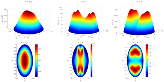
Figure 3. The three-dimensional and axial projection drawing particle distribution when $n=1/2$, $n=1$ and $n=3$.

Figure 4 presents the influence of parameter $\xi$ on the particle distributions for $t=1$, $f(x,y,t)=0$, $d_1\left(x,y\right)=\frac{1-x}{2}\delta \left(y\right)$, $d_2\left(x,y\right)=\frac{1+x}{2}\delta \left(y\right)$, $e(x,y)=x^2+y^2+1$, ${\phi }_1\left(\beta \right)=1$ and ${\phi }_0\left(\alpha \right)=1$. As the relaxation parameter increases from $\xi =0$ to $\xi =1$, the central region of the particle distribution begins to cave inward, which indicates that the distributions have a wave characteristic. The larger the relaxation parameter is, the stronger the wave characteristic will be. The reason is that the relaxation parameter is added on the distributed-order time-fractional derivative of order $(1,2)$, which possesses the wave characteristics. With an increase in the relaxation parameter, the fractional derivative of order $(1,2)$ with the wave characteristic plays a greater role in the particles’ transport.

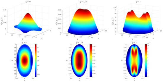
Figure 4. The three-dimensional and axial projection drawing particle distribution when $\xi =0$, $\xi =1/2$ and $\xi =1$.

6. Conclusions

In this paper, we presented an original distributed-order time- and space-fractional diffusion-wave equation to analyze the anomalous diffusion in comb structures. The solution of the governing equation was obtained using the finite element method for the case where the coefficients are taken as constant. Two examples were given: one was in a rectangular domain and the other one was in an elliptical domain. In the two examples, the $H_{\gamma }$ error, $L_2$ error and convergence order of h with $\tau =\frac{1}{1000}$ at $t=1$ subject to different weight coefficients showed that the results demonstrated the effectiveness of the numerical method. For the elliptical domain, the influence of the involved parameters, such as the relaxation parameter and the weight coefficient on the particle distribution, were analyzed, and the physical meaning of the diffusion-wave characteristics was discussed in detail.

References

- Iomin, A.; Méndez, V.; Horsthemke, W. Fractional Dynamics in Comb-Like Structures; World Scientific: Singapore, 2018. [Google Scholar]
- Iomin, A.; Méndez, V. Reaction-subdiffusion front propagation in a comblike model of spiny dendrites. Phys. Rev. E 2013, 88, 012706. [Google Scholar] [CrossRef] [PubMed]
- Iomin, A.; Zaburdaev, V.; Pfohl, T. Reaction front propagation of actin polymerization in a comb-reaction system. Chaos Solitons Fract. 2016, 92, 115–122. [Google Scholar] [CrossRef]
- Méndez, V.; Iomin, A. Comb models for transport along spiny dendrites. In Handbook of Applications of Chaos Theory; CRC Press: Boca Raton, FL, USA, 2014. [Google Scholar]
- Méndez, V.; Iomin, A. Comb-like models for transport along spiny dendrites. Chaos Solitons Fract. 2013, 53, 46–51. [Google Scholar] [CrossRef]
- Iomin, A. Toy model of fractional transport of cancer cells due to self-entrapping. Phys. Rev. E 2006, 73, 061918. [Google Scholar] [CrossRef] [PubMed]
- Iomin, A. A toy model of fractal glioma development under RF electric field treatment. Eur. Phys. J. E 2012, 35, 42–46. [Google Scholar] [CrossRef]
- Arkhincheev, V.E.; Baskin, E.M. Anomalous diffusion and drift in a comb model of percolation clusters. Zh. Eksp. Teor. Fiz. 1991, 100, 292–300. [Google Scholar]
- Baskin, E.; Iomin, A. Superdiffusion on a Comb Structure. Phys. Rev. Lett. 2004, 93, 120603. [Google Scholar] [CrossRef]
- Christov, C.I.; Jordan, P.M. Heat conduction paradox involving second-sound propagation in moving media. Phys. Rev. Lett. 2015, 94, 154301. [Google Scholar] [CrossRef]
- Compte, A.; Metzler, R. The generalized Cattaneo equation for the description of anomalous transport processes. J. Phys. A-Math. Gen. 1997, 30, 7277–7289. [Google Scholar] [CrossRef]
- Iomin, A. Fractional kinetics of glioma treatment by a radio-frequency electric field. Eur. Phys. J. Spec. Top. 2013, 222, 1875–1884. [Google Scholar] [CrossRef]
- Liu, F.; Yang, Q.; Turner, I. Two new implicit numerical methods for the fractional cable equation. J. Comput. Nonlin. Dyn. 2011, 6, 011009. [Google Scholar] [CrossRef]
- Qi, H.T.; Xu, H.Y.; Guo, X.W. The Cattaneo-type time fractional heat conduction equation for laser heating. Comput. Math. Appl. 2013, 66, 824–831. [Google Scholar] [CrossRef]
- Oloniiju, S.D.; Goqo, S.P.; Sibanda, P. A chebyshev spectral method for heat and mass transfer in mhd nanofluid flow with space fractional constitutive model. Front. Heat Mass Transf. 2019, 13, 13–19. [Google Scholar] [CrossRef]
- Eab, C.H.; Lim, S.C. Fractional Langevin equation of distributed order. Phys. Rev. E 2011, 83, 031136. [Google Scholar] [CrossRef]
- Caputo, M. Distributed order differential equations modeling dielectric induction and diffusion. Fract. Calc. Appl. Anal. 2001, 4, 421–442. [Google Scholar]
- Bai, Y.; Wan, S.; Zhang, Y.; Wang, X. Unsteady Falkner-Skan flow of fractional Maxwell fluid towards a stretched wedge with buoyancy effects. Phys. Scripta 2022, 98, 015218. [Google Scholar] [CrossRef]
- Elwakil, S.A.; Zahran, M.A.; Abulwafa, E.M. Fractional (space-time) diffusion equation on comb-like model. Chaos Solitons Fract. 2004, 20, 1113–1120. [Google Scholar] [CrossRef]
- Ervin, V.J.; Roop, J.P. Variational formulation for the stationary fractional advection dispersion equation. Numer. Meth. Part. D. E. 2006, 22, 558–576. [Google Scholar] [CrossRef]
- Bu, W.; Tang, Y.; Yang, J. Galerkin finite element method for two-dimensional Riesz space fractional diffusion equations. J. Comput. Phys. 2014, 276, 26–38. [Google Scholar] [CrossRef]
- Bu, W.; Tang, Y.; Wu, Y.; Yang, J. Finite difference/finite element method for twodimensional space and time fractional Bloch-Torrey equations. J. Comput. Phys. 2015, 293, 264–279. [Google Scholar] [CrossRef]
- Yang, Z.; Yuan, Z.; Nie, Y.; Wang, J.; Zhu, X.; Liu, F. Finite element method for nonlinear Riesz space fractional diffusion equations on irregular domains. J. Comput. Phys. 2017, 330, 863–883. [Google Scholar] [CrossRef]
- Hao, Z.; Park, M.; Lin, G.; Cai, Z. Finite element method for two-sided fractional differential equations with variable coeffificients: Galerkin approach. J. Sci. Comput. 2019, 79, 700–717. [Google Scholar] [CrossRef]
- Wang, H.; Yang, D. Wellposedness of variable-coefficient conservative fractional elliptic differential equations. Siam J. Numer. Anal. 2013, 51, 1088–1107. [Google Scholar] [CrossRef]
- Wang, H.; Yang, D.; Zhu, S. Inhomogeneous Dirichlet boundary-value problems of space-fractional diffusion equations and their finite element approximations. Siam J. Numer. Anal. 2014, 52, 1292–1310. [Google Scholar] [CrossRef]
- Ervin, V.J.; Roop, J.P. Variational solution of fractional advection dispersion equations on bounded domains in Rd. Numer. Methods Partial Differ. Equat. 2007, 23, 256–281. [Google Scholar] [CrossRef]
- Roop, J.P. Variational Solution of the Fractional Advection Dispersion Equation. Ph.D. Thesis, Clemson University, Clemson, SC, USA, 2004. [Google Scholar]
- Moghaddam, B.P.; Machado, J.A.T.; Morgado, M.L. Numerical approach for a class of distributed order time fractional partial differential equations. Appl. Numer. Math. 2019, 136, 152–162. [Google Scholar] [CrossRef]
- Sun, Z.; Wu, X. A fully discrete difference scheme for a diffusion-wave system. Appl. Numer. Math. 2006, 56, 193–209. [Google Scholar] [CrossRef]
- Fan, H.; Zhao, Y.; Wang, F.; Shi, Y.; Tang, Y. A superconvergent nonconforming mixed FEM for multi-term time-fractional mixed diffusion and diffusion-wave equations with variable coefficients. East Asian J. Appl. Math 2021, 11, 63–92. [Google Scholar] [CrossRef]
- Geuzaine, C.; Remacle, J.F. Gmsh: A 3-D flnite element mesh generator with built-in pre-and post-processing facilities. Int. J. Numer. Meth. Eng. 2009, 79, 1309–1331. [Google Scholar] [CrossRef]
Disclaimer/Publisher’s Note: The statements, opinions and data contained in all publications are solely those of the individual author(s) and contributor(s) and not of MDPI and/or the editor(s). MDPI and/or the editor(s) disclaim responsibility for any injury to people or property resulting from any ideas, methods, instructions or products referred to in the content. |
© 2023 by the authors. Licensee MDPI, Basel, Switzerland. This article is an open access article distributed under the terms and conditions of the Creative Commons Attribution (CC BY) license (https://creativecommons.org/licenses/by/4.0/).