Article

Mathematical Modeling of COVID-19 with Vaccination Using Fractional Derivative: A Case Study

by
Tian-Chuan Sun
1,
Mahmoud H. DarAssi
2,
Wafa F. Alfwzan
3,
Muhammad Altaf Khan
4,5,*,
Abdulaziz Saad Alqahtani
6,
Saeed S. Alshahrani
7 and
Taseer Muhammad
8
1
School of Marxism (Department of Public Teaching and Researching), Huzhou College, Huzhou 313000, China
2
Department of Basic Sciences, Princess Sumaya University for Technology, Amman 11941, Jordan
3
Department of Mathematical Sciences, College of Science, Princess Nourah Bint Abdulrahman University, P.O. Box 84428, Riyadh 11671, Saudi Arabia
4
Faculty of Natural and Agricultural Sciences, University of the Free State, Bloemfontein 9300, South Africa
5
Department of Mathematics, Faculty of Science and Technology, Universitas Airlangga, Surabaya 60115, Indonesia
6
Department of Internal Medicine, College of Medicine, Najran University, Najran 55461, Saudi Arabia
7
Department of Surgery, College of Medicine, Najran University, Najran 55461, Saudi Arabia
8
Department of Mathematics, College of Sciences, King Khalid University, Abha 61413, Saudi Arabia
*
Author to whom correspondence should be addressed.
Fractal Fract. 2023, 7(3), 234; https://doi.org/10.3390/fractalfract7030234
Submission received: 14 December 2022 / Revised: 13 February 2023 / Accepted: 24 February 2023 / Published: 6 March 2023
(This article belongs to the Special Issue Fractional Order Modeling in Interdisciplinary Applications)

Abstract

:
Vaccination against any infectious disease is considered to be an effective way of controlling it. This paper studies a fractional order model with vaccine efficacy and waning immunity. We present the model’s dynamics under vaccine efficacy, the impact of immunization, and the waning of the vaccine on coronavirus infection disease. We analyze the model under their equilibrium points. The model under the equilibrium points is discussed and proven that it is locally asymptotically stable if R v is lesser than unity. We present the backward bifurcation hypothesis of the model and show that there is a parameter β 2 that causes the backward bifurcation in the imperfect vaccine model. We show certain assumptions when ψ = 1 for the imperfect vaccine case; the model is both stable globally asymptotically at the disease-free ( R 0 1 ) and endemic cases ( R 0 > 1 ). By using infected cases from the recent wave throughout Pakistan, we shall estimate the model parameters and calculate the numerical value of the basic reproductive number R 0 1.2591 . We present the comprehensive graphical results for the realistic parameter values and show many useful suggestions regarding the elimination of the infection from society. The vaccination efficacy that provides an important role in disease elimination is discussed in detail.

1. Introduction

Coronavirus, since the beginning of March 2020 till now, has been producing new infections, and until now, the number of recorded cases that have been documented in Pakistan is 1,575,186 [1]. Among these infected cases, 98% have recovered, which is 98% of the total cases, while 2% are death cases, 30,631, have been reported. Since March 2020 till now, different waves of coronavirus infection have been observed, while the latest (sixth wave) was recorded in May 2022–September 2022 [1]. If we can look at the data given in [1], earlier, there were several cases of infection, and gradually, in the latest wave, the number of infected cases significantly decreased. One of the reasons is that earlier people were not aware of the issue of not getting vaccines in the market.
Vaccination is a useful tool to protect humans against disease. The coronavirus infection, and its emergence in the world as a new virus, was a big challenge because there was no treatment or control, and vaccines are available in the market. With the efforts of researchers and biologists in the development of vaccines, coronavirus infection has been reduced by a significant number of cases. Some mathematical models that used the control startles are given in [2,3]. The modeling in [2] depicts coronavirus infection with the use of control methods. The fractional order model given in [3] has been considered in the study of coronavirus, considering different control mechanisms.
The vaccines related to coronavirus that are available in the market are different types, such as Moderna, Pfizer, Johnson and Johnson, chines vaccines, etc. It should be noted that none of the vaccines developed so far is 100% effective, and still, there is a waning vaccine rate. Therefore, in the recently developed vaccines, there is also a warning about vaccines. In some less-developed countries of the world with poor financial health funds, the development of vaccines against coronavirus infection is not possible. A total of 70 countries of the world with low income have a vaccination rate of 1–10 individuals [4]. International organizations are trying to provide vaccines with equal distribution to curb coronavirus. It should be underlined that the inequitable distribution of vaccinations cannot be resolved in a short period of time. As a result, more realistic immunization rates must be investigated.
Vaccines are considered the most effective controls for disease elimination, but they are limited and affected in the implementation process by various factors. Researchers from various countries around the world regarding vaccine strategies have provided useful published materials in the literature. For example, the authors in [5] developed vaccination strategies for single and double-dose vaccination and studied their epidemic disease dynamics. The authors in [6] developed a vaccination model considering the treatment and vaccination saturating function with strategies. Vaccines containing diseases and the role of media effects have been explored in [7]. Studying the vaccination model with secondary infection after vaccine coverage and immunization is explored in [8]. Vaccination and treatment impacts on coronavirus have been studied in [9]. The availability of vaccines and the vaccine strategies’ impact on disease elimination is studied in [10,11,12]. A series of mathematical models for the coronavirus epidemic, studying their bifurcation and local and global asymptotical dynamics, have been discussed in [13,14]. The study of the vaccination model under vaccine immunization and their efficacy have been discussed in detail in [15].
Mathematical models to understand infectious diseases and especially COVID-19 with integer and non-integer orders are documented in the literature, see [16,17,18]. For example, a model with real data has been formulated and studied in [19]. Using the distributions of the cases with asymptomatic and symptomatic compartments are shown through a mathematical model in [20]. The coronavirus model with treatment is discussed in [21]. The vaccine model for coronavirus and their controlling strategies is shown in [22]. The algorithm for the COVID-19 is used to identify the undetected cases is discussed in [23]. A non-integer system to analyze the coronavirus using the real cases in Pakistan is explored in [24]. The formulation of the SARS-Cov-2 in fractional derivative to understand the new omicron variant is shown in [25]. The discussion on the second wave of the coronavirus infection and a stability analysis has been investigated in [26]. The reported coronavirus cases in India through a fractional order model are studied in [27]. Some more related applications of fractional calculus can be seen in [28,29,30,31]. In [28], neural network dynamics have been discussed. The authors in [29] used the IIR filter to obtain results for fractional order equations for grid-tied inverters. The dynamics of the prey-predator system have been analyzed using the fractional derivative and studied in [30]. A numerical investigation of the Fractional Step-Down option system has been explored in [31]. The cholera dynamics under the fractional differential equation have been analyzed in [32]. The coronavirus dynamics spread under fractional calculus has been analyzed in [33]. The dynamics of the monkeypox disease using arbitrary calculus is shown in [34].
The arrangement of the work is given as follows: Detailed materials regarding the fractional operator and the formulation of the problem in both integer and non-integer order are presented in Section 2. The analysis of the vaccination model and the backward bifurcation is discussed in Section 3. The stability analysis of the system is given in Section 4. Estimations of the parameters using the recent wave of COVID-19 in Pakistan have been considered in Section 5. Numerical results and the main achievements of the present work are discussed in Section 6 and Section 7, respectively.

2. Model Formulation and Basic Relations to Fractional Calculus

The necessary results that shall be used later in this work are given below.
Definition 1 
([35]). The definition of a Caputo derivative under a function g C n ( [ 0 , + ) , R ) , ( n 1 < η n ) (η is fractional order) can be written as,
D η g ( t ) = 1 Γ ( n η ) 0 t ( t τ ) n η 1 g ( n ) ( τ ) d τ , t > 0 ,
Definition 2 
([35]). When η > 0 then the Riemann–Liouville fractional integral of a function g : R + R can be shown as,
I η g ( t ) = 1 Γ ( η ) 0 t ( t τ ) η 1 g ( τ ) d τ ,
where Γ ( η ) is defined to be the Euler Gamma function [36].
Lemma 1. 
For η ( 0 , 1 ] , let g ( t ) C ( [ u , v ] ) and D η g ( t ) ( u , v ] . Then it holds
g ( t ) = g ( u ) + 1 Γ ( η ) D η g ( ξ ) ( t u ) η ,
ξ [ 0 , 1 ] , t ( u , v ] .

2.1. Model Formulation

We consider the coronavirus infection with vaccine efficacy through a mathematical modeling approach. The population of human is denoted by N ( t ) and divided further into six subgroups. These groups are defined as: The vulnerable population is signified by S ( t ) , which has the ability to be affected by coronavirus infection. The individuals in this group are not immunized. Vaccinated individuals against the coronavirus are given by V ( t ) , E ( t ) is the exposed individuals in an exposed period. After healthy individuals have close contact with people who have the coronavirus infection, people who are clinically identified to be asymptomatically infected with no clinical disease symptoms of coronavirus infection are called asymptomatic infected, shown by A ( t ) . Individuals who exhibit obvious illness signs are said to be symptomatically infected. I ( t ) . Those who have recovered from coronavirus illness are gathered in R ( t ) . Therefore, we shall write N ( t ) = S ( t ) + V ( t ) + E ( t ) + A ( t ) + I ( t ) + R ( t ) . Because of the immunological reaction induced by vaccination, persons in vaccinated populations cannot become infected with the virus. With the gradual decrease in the indicated vaccine antibodies with the passage of time, a number of people may become susceptible to being infected with the virus. With these observations, our above discussions lead to the following evolutionary nonlinear ordinary differential equations:
d S d t = Π ( β 1 I + β 2 A ) S N ( ω + μ ) S ( t ) + κ R + θ V ( t ) , d V d t = ω S ( 1 ψ ) ( β 1 I + β 2 A ) V N ( θ + μ ) V , d E d t = ( β 1 I + β 2 A ) S N + ( 1 ψ ) ( β 1 I + β 2 A ) V N ( δ + μ ) E , d A d t = q δ E ( μ + ρ 1 ) A , d I d t = ( 1 q ) δ E ( μ + d + ρ ) I , d R d t = ρ I + ρ 1 A ( κ + μ ) R ,
with the initial conditions given by,
S ( 0 ) = S 0 0 , V ( 0 ) = V 0 0 , E ( 0 ) = E 0 0 , A ( 0 ) = A 0 0 , I ( 0 ) = I 0 0 , R ( 0 ) = R 0 0 .
The parameter Π defines the susceptible population’s birth rate, whereas μ in each component of the system represents the natural death rate. Susceptible persons become infected after coming into contact with infected people (asymptomatic or symptomatic) via the transmission channel provided by β 1 and β 2 . The contact between the healthy and symptomatic infected is shown by route β 1 , while β 2 is responsible for the disease progression as a result of healthy people coming into contact with asymptomatic infected people. The vaccination rate of healthy people is given by ω , while θ is the vaccine’s waning immunity rate. The natural loss of immunity of the recovered individuals is given by κ . We considered the imperfect vaccines and the fact that there is no perfect vaccine on the market to curb coronavirus infection. Therefore, parameter ψ is the vaccine efficacy rate. If ψ = 1 , then the vaccine is perfect; otherwise it is imperfect. The exposed period of individuals after close contact with asymptomatic or symptomatic is shown by δ . The part of people that do not possess disease symptoms shall join the asymptomatic infected class A with the rate given by q δ , while the individuals that have clear infection symptoms join the symptomatic infected class I with the rate ( 1 q ) δ . The rate of recovery of asymptomatic infected patients is provided by ρ 1 , and those recovered from symptomatic infection are given by ρ . The coronavirus infection has produced a high number of death cases around the world, so the disease mortality rate of symptomatic infected people is given by d.

2.2. Model Positivity and Boundedness

This section investigates model (3)’s solution’s positivity and boundedness. It is important to demonstrate that the model solution at a non-negative beginning value is always non-negative for t > 0 . The following theorem gives us the results:
Theorem 1. 
Let U ( t ) = ( S ( t ) , V ( t ) , E ( t ) , A ( t ) , I ( t ) , R ( t ) ) for all t 0 be the positive solution of model (3) with the initial conditions (4). Then the solution of system (3) is non-negative for each t > 0 .
Proof. 
Let U ( t ) = min { S ( t ) , V ( t ) , E ( t ) , A ( t ) , I ( t ) , R ( t ) } , where S ( t ) , V ( t ) , E ( t ) , A ( t ) , I ( t ) , and R ( t ) are the associated positive solutions of system (3). We know U ( 0 ) > 0 . Let us consider that there exists t 1 > 0 such that U ( t 1 ) = 0 and U ( t ) > 0 for any t [ 0 , t 1 ) . If M ( t 1 ) = S ( t 1 ) , then V ( t ) 0 , E ( t ) 0 , A ( t ) 0 , I ( t ) 0 , and R ( t ) 0 for any t [ 0 , t 1 ) . Consider the first equation of system (3) for any t [ 0 , t 1 ) ,
d S ( t ) d t = Π ( β 1 I + β 2 A ) S N ( ω + μ ) S ( t ) + κ R + θ V ( t ) , Π ( λ ( t ) + ( ω + μ ) ) S ( t ) .
We shall write the following,
d S ( t ) d t + ( λ ( t ) + ( ω + μ ) ) S ( t ) Π .
We get after utilizing the integration method,
d d t S ( t ) exp 0 t ( λ ( t ) + ω + μ ) d z Π exp 0 t ( λ ( t ) + ω + μ ) d z .
Finally, it leads to the following,
S t 1 S ( 0 ) exp 0 t 1 ( λ ( t ) + ω + μ ) d z + exp 0 t 1 ( λ ( t ) + ω + μ ) d z × Π 0 t 1 exp 0 x ( λ ( z ) + ω + μ ) d z d x > 0 ,
that leads to a contradiction, and hence we can get S ( t ) 0 for any t 0 . We can have similar result for V ( t ) 0 ,
d V d t = ω S ( 1 ψ ) ( β 1 I + β 2 A ) V N ( θ + μ ) V , d V d t ( 1 ψ ) ( λ ( t ) + θ + μ ) V , V ( t ) V ( 0 ) e ( λ ( t ) + θ + μ ) t .
The result for E ( t ) is,
d E d t = λ ( t ) S + ( 1 ψ ) λ ( t ) V ( δ + μ ) E , d E d t ( δ + μ ) E , E ( t ) E ( 0 ) e ( δ + μ ) t .
For A ( t ) , we give the following,
d A d t = q δ E ( μ + ρ 1 ) A , d A d t ( μ + ρ 1 ) A , A ( t ) A ( 0 ) e ( ρ 1 + μ ) t .
We shall get the result for I ( t ) and R ( t ) , follows the same stepping used above,
d I d t = ( 1 q ) δ E ( μ + d + ρ ) I , d I d t ( μ + d + ρ ) I , I ( t ) I ( 0 ) e ( ρ + μ + d ) t ,
d R d t = ρ I + ρ 1 A ( μ + κ ) R , d R d t ( μ + κ ) R , R ( t ) R ( 0 ) e ( κ + μ ) t .
This ends the proof of the positivity of the model variables. To show the boundedness of model (3), we just add the model equations and receive
d N ( t ) d t = Π μ N ( t ) d N ( t ) Π μ N .
The solution is given for t ,
lim t sup N ( t ) Π μ .
With the help of the positivity and boundedness of the result shown in the theorem above, now we can define the feasible region. The biologically feasible region where the model solutions are positive invariant and bounded are given as
Γ = ( S , V , E , A , I , R ) R + 6 : S , V , E , A , I , R 0 , 0 N ( t ) Π μ .

2.3. Caputo Fractional Order Model

The fractional system in science and engineering areas and especially in epidemiology, has great importance in order to study heredity and memory effects, which shall not be found in integer-order models. It should be worth mentioning that many definitions exist in the literature regarding the fractional derivative, and everyone has their own importance; we use the definition of Caputo derivative to model coronavirus disease with vaccinations. Here, we apply the Caputo fractional order definition given above and obtain the fractional version of the above system (12) given by:
D t α S ( t ) = Π ( β 1 I + β 2 A ) S N ( ω + μ ) S ( t ) + κ R + θ V ( t ) , D t α V ( t ) = ω S ( 1 ψ ) ( β 1 I + β 2 A ) V N ( θ + μ ) V , D t α E ( t ) = ( β 1 I + β 2 A ) S N + ( 1 ψ ) ( β 1 I + β 2 A ) V N ( δ + μ ) E , D t α A ( t ) = q δ E ( μ + ρ 1 ) A , D t α I ( t ) = ( 1 q ) δ E ( μ + d + ρ ) I , D t α R ( t ) = ρ I + ρ 1 A ( κ + μ ) R ,
where the initial conditions are
S ( 0 ) = S 0 0 , V ( 0 ) = V 0 0 , E ( 0 ) = E 0 0 , A ( 0 ) = A 0 0 , I ( 0 ) = I 0 0 , R ( 0 ) = R 0 0 .
In the next part, we show the findings for the fractional model.

3. Analysis of the Equilibrium Points

This section briefly explores the possible equilibrium points of model (12) and studies the possibilities of the backward bifurcation phenomenon. We shall begin with the calculation of the disease-free case.

3.1. Disease-Free Equilibrium (DFE)

The disease-free equilibrium of model (12) is shown by P 0 and is given by
P 0 = ( S 0 , V 0 , 0 , 0 , 0 , 0 ) = Π ( θ + μ ) μ ( θ + μ + ω ) , Π ω μ ( θ + μ + ω ) , 0 , 0 , 0 , 0 .
Next, we calculate the basic reproductive number which has a key role in epidemic models.

3.2. Basic Reproduction Number

The reproductive number has significant advantages in disease models. One of the important roles of this is to characterize the disease dynamics. Usually, when its numerical value is less than unity, the disease is regarded to be a controllable whole in the case of exceeds unity it might be spread among other community members. Also, it is very important to mention that when its value is exactly equal to one then there may be a backward bifurcation. We shall give the mathematical computation of the basic vaccine reproduction number of system (12) using the approach shown in [37] and is given by:
F = 0 V 0 ( 1 ψ ) β 2 S 0 + V 0 + S 0 β 2 S 0 + V 0 V 0 ( 1 ψ ) β 1 S 0 + V 0 + S β 1 S 0 + V 0 0 0 0 0 0 0 , and V = ( δ + μ ) 0 0 q δ ( μ + ρ 1 ) 0 ( 1 q ) δ 0 ( d + μ + ρ ) .
Therefore, we have the results after using ρ ^ [ F V 1 ] and the required vaccine basic reproduction number R v ,
R v = β 1 δ ( 1 q ) ( θ + μ ψ ω + ω ) ( δ + μ ) ( d + μ + ρ ) ( θ + μ + ω ) + β 2 δ q ( θ + μ ψ ω + ω ) ( δ + μ ) ( μ + ρ 1 ) ( θ + μ + ω ) , = R v 1 + R v 2 .
The expression of R 0 describes the number of individuals that an infected person infects. When ψ = 1 and ω = θ = 0 , then R v reduces to
R 0 = β 1 δ ( 1 q ) ( δ + μ ) ( d + μ + ρ ) + β 2 δ q ( δ + μ ) ( μ + ρ 1 ) ,
is the basic reproduction number in the absence of vaccination. For disease elimination, it can be useful if R 0 < 1 .

3.3. Endemic Equilibria

Here, we shall determine the existence of endemic equilibria and determine that there may be possibilities of the backward bifurcation. It should be noted that the perfect vaccine model does not possess the backward bifurcation that the imperfect vaccines causes. The endemic equilibria of system (12) is denoted by P 1 , and P 1 = ( S , V , E , A , I , R ) which shall be obtained as given by,
D t α S ( t ) = 0 , D t α V ( t ) = 0 , D t α E ( t ) = 0 , D t α A ( t ) = 0 , D t α I ( t ) = 0 , D t α R ( t ) = 0 .
Solving (13) at the steady-state, we have the result below,
S = Π + κ R + θ V λ + μ + ω , V = ω S θ + λ ( 1 ψ ) + μ , E = λ S + λ V ( 1 ψ ) δ + μ , A = δ q E ρ 1 + μ , I = δ ( 1 q ) E d + μ + ρ , R = ρ 1 A + ρ I κ + μ .
We consider the expression in (14) and insert it into,
λ = β 2 A + β 1 I N ,
where N = S + V + E + A + I + R , we obtain,
b 1 λ 2 + b 2 λ + b 3 = 0 ,
where
b 1 = ( 1 ψ ) ( ρ 1 + μ ) ( ( κ + μ ) ( d + μ + δ ( 1 q ) + ρ ) + δ ( 1 q ) ρ ) + δ q ( 1 ψ ) ( d + μ + ρ ) ( ρ 1 + κ + μ ) , b 2 = ( 1 ψ ) ( d + μ + ρ ) ( κ + μ ) ( ρ 1 + μ ) ( δ + μ + ω ) + δ q ω β 2 + δ ρ 1 q ω + δ ( 1 q ) ( 1 ψ ) ( ρ 1 + μ ) ω β 1 ( κ + μ ) + ρ ω + ( θ + μ ) ( d + μ + ρ ) × ( ( κ + μ ) ( ρ 1 + μ + δ q ) + δ ρ 1 q ) + δ ( 1 q ) ( ρ 1 + μ ) ( θ + μ ) ( κ + μ + ρ ) , b 3 = ( δ + μ ) ( ρ 1 + μ ) ( κ + μ ) ( d + μ + ρ ) ( θ + μ + ω ) ( θ + μ + ( 1 ψ ) ω ) ( 1 R v ) .
We can see that b 1 > 0 , and b 3 can be positive if R v < 1 while it is negative for R v > 1 . We cannot say about the positive value of b 2 , so there should be some conditions where the quadratic Equation (15) can show the positive and unique endemic equilibrium of model (12). We shall provide the statement below:
Theorem 2. 
Model (12) has:
(i)
a unique endemic equilibrium exists if b 3 < 0 R v > 1 ,
(ii)
a unique endemic equilibrium exists if b 2 < 0 and b 3 = 0 R v = 1 ,
(iii)
two endemic equilibria exist if b 3 > 0 R v < 1 , b 2 < 0 and its related discriminant is positive
(iv)
there is no possible equilibria other than the above cases.
When R v > 1 , the first portion of Theorem 2 clearly indicates the presence of a unique positive endemic equilibrium. Furthermore, we can see from the third part of Theorem 2 that there is a backward bifurcation in the coronavirus vaccination model (12). The presence of backward bifurcation in disease models indicates that the stable disease-free equilibrium coexists with the endemic equilibrium, and hence there is no chance of the model achieving global asymptotical stability in the disease-free scenario. In such a circumstance, the disease will be present in the community for an extended period of time, and immunizations, preventive, and other required control measures can be utilised to eradicate the infection. For mathematical results of the backward bifurcation and simulation results, we shall use the discriminant set as follows, b 2 2 4 b 1 b 3 = 0 . Further solving the discriminant to get the critical values of R v can be shown by R c , which is shown by
R c = 1 b 2 2 4 b 1 ( δ + μ ) ( κ + μ ) ( d + μ + ρ ) ( θ + μ + ω ) .
We can see that there exists backward bifurcation for R v such that R c < R v < 1 . The backward bifurcation occurs for β 2 = 0.4827 , while the rest of the values are the same as shown in Table 1. The bifurcation result is shown in Figure 1, where β 2 is the bifurcation parameter causing backward bifurcation in the vaccination model with the imperfect vaccine. Because of the the imperfect vaccine, the disease-free equilibrium coexists alongside the stable endemic equilibrium. In models where backward bifurcation exists, then it needs to reduce the threshold quantity to less than unity in order to control the disease spread via vaccination, prevention, educating individuals against the disease, etc. It should be noted that when ψ = 1 (perfect vaccine), then the presence of backward bifurcation is ruled out.

4. Stability Analysis

This section discusses the asymptotical stability of model (12).
Theorem 3. 
When η ( 0 , 1 ] , and R 0 < 1 , then model (12) is locally asymptotically stable if all the eigenvalues λ k , for k = 1 , , 6 satisfy
| a r g ( λ k ) | > η π 2 .
Proof. 
We have the Jacobian matrix at P 0 ,
J = ( μ + ω ) θ 0 β 2 S 0 S 0 + V 0 β 1 S 0 S 0 + V 0 κ ω ( θ + μ ) 0 ( 1 ψ ) β 2 V 0 S 0 + V 0 ( 1 ψ ) β 1 V 0 S 0 + V 0 0 0 0 ( δ + μ ) ( 1 ψ ) β 2 V 0 S 0 + V 0 + β 2 S 0 S 0 + V 0 ( 1 ψ ) β 1 V 0 S 0 + V 0 + β 1 S 0 S 0 + V 0 0 0 0 q δ ( ρ 1 + μ ) 0 0 0 0 ( 1 q ) δ 0 ( d + μ + ρ ) 0 0 0 0 g ρ ( κ + μ ) .
We have the characteristic equation for J, given by
λ 6 + c 1 λ 5 + c 2 λ 4 + c 3 λ 3 + c 4 λ 2 + c 5 λ + c 6 = 0 ,
where
c 1 = d + δ + ρ 1 + θ + κ + 6 μ + ρ + ω , c 2 = ( θ + μ ) ( d + δ + g + κ + 4 μ + ρ ) + ( μ + ω ) ( d + δ + ρ 1 + κ + 4 μ + ρ ) + ( κ + μ ) ( d + δ + g + 3 μ + ρ ) + ( ρ 1 + μ ) ( d + μ + ρ ) + μ ( θ + μ + ω ) + ( δ + μ ) ( d + μ + ρ ) ( 1 R v 1 ) + ( δ + μ ) ( ρ 1 + μ ) ( 1 R v 2 ) , c 3 = ( κ + μ ) ( ( d + μ + ρ ) ( ρ 1 + θ + 3 μ + ω ) + ( δ + ρ 1 + 2 μ ) ( θ + 2 μ + ω ) ) + ( ρ 1 + μ ) ( d + μ + ρ ) ( θ + 2 μ + ω ) + μ ( θ + μ + ω ) ( d + δ + ρ 1 + κ + 4 μ + ρ ) + ( δ + μ ) ( d + μ + ρ ) ( θ + κ + 3 μ + ω ) ( 1 R v 1 ) + ( δ + μ ) ( ρ 1 + μ ) ( d + μ + ρ ) ( 1 R v ) + ( δ + μ ) ( ρ 1 + μ ) ( θ + κ + 3 μ + ω ) ( 1 R v 2 ) , c 4 = μ ( θ + μ + ω ) ( ( κ + μ ) ( d + δ + ρ 1 + 3 μ + ρ ) + ( ρ 1 + μ ) ( d + μ + ρ ) ) + ( ρ 1 + μ ) ( κ + μ ) ( d + μ + ρ ) ( θ + 2 μ + ω ) + ( δ + μ ) ( g + μ ) ( d + μ + ρ ) × ( θ + κ + 3 μ + ω ) ( 1 R v ) + ( θ + μ ) ( κ + μ ) + μ ( θ + μ + ω ) + ( κ + μ ) ( μ + ω ) 1 R v 1 + ( δ + μ ) ( g + μ ) ( ( κ + μ ) ( θ + 2 μ + ω ) + μ ( θ + μ + ω ) ) ( 1 R v 2 ) , c 5 = μ ( δ + μ ) ( κ + μ ) ( θ + μ + ω ) ( ( 1 R v 1 ) ( d + μ + ρ ) + ( 1 R v 2 ) ( ρ 1 + μ ) ) + ( δ + μ ) ( g + μ ) ( d + μ + ρ ) ( ( κ + μ ) ( θ + 2 μ + ω ) + μ ( θ + μ + ω ) ) ( 1 R v ) + μ ( ρ 1 + μ ) ( κ + μ ) ( d + μ + ρ ) ( θ + μ + ω ) , c 6 = μ ( κ + μ ) ( θ + μ + ω ) ( 1 R v ) .
The coefficients c 1 > 0 and c k , for k = 2 , , 6 are positive when R v < 1 . Further, it is easy to satisfy the Routh–Hurtwiz criteria using any algebraic computation software. We conclude that the disease-free equilibrium of system (12) is locally asymptotically stable when R v < 1 . □

4.1. Global Stability

We can consider the vaccination model to show their global asymptomatic stability. We consider a special case when ψ = 1 , to show that the vaccination model is globally asymptotically stable.
Theorem 4. 
Vaccination model (3) when ψ = 1 for η ( 0 , 1 ] is globally asymptotically stable if R 0 1 .
Proof. 
Consider the below Lyapunov function
L = g 1 E + g 2 A + g 3 I ,
where
g 1 = ( μ + ρ 1 ) , g 2 = β 2 , g 3 = β 1 ( μ + ρ 1 ) d + μ + ρ .
Taking the time derivative of L and using the equations from (3), we have
D t α L = g 1 [ ( β 1 I + β 2 A ) S N ( δ + μ ) E ] + g 2 [ q δ E ( μ + ρ 1 ) A ] + g 3 [ ( 1 q ) δ E ( μ + d + ρ ) I ] .
This leads to the result below,
D t α L = [ g 1 β 1 S N g 3 ( μ + d ρ ) ] I + [ g 1 β 2 S N g 2 ( μ + ρ 1 ) ] A + [ g 2 δ q + g 3 ( 1 q ) δ g 1 ( δ + μ ) ] E .
We using the fact that ( S ( t ) N ( t ) ) , and receive
D t α L β 1 δ ( 1 q ) ( δ + μ ) ( d + μ + ρ 1 ) + δ q β 2 ( δ + μ ) ( μ + ρ 1 ) 1 ( δ + μ ) ( μ + ρ 1 ) E , ( δ + μ ) ( μ + ρ 1 ) ( R 0 1 ) E .
Thus, if R 0 1 , then D t α L 0 , and if E ( t ) = 0 , then D t α L = 0 . Using E ( t ) = 0 in system (3), it can be seen that model (3) approaches the disease-free equilibrium. Therefore, LaSalle’s Invariance Principle ensures that the vaccination model (3) when ψ = 1 is globally asymptotically stable. □

4.2. Global Stability of Endemic Equilibrium for Special Case ( ψ = 1 , κ = 0 )

We use the following results in the proof of endemic equilibrium P 1 :
Π = ( β 1 I + β 2 A ) S + ( ω + μ ) S θ V , ω = ( θ + μ ) V S , ( δ + μ ) = ( β 1 I + β 2 A ) S E , ( μ + ρ 1 ) q δ = E A , ( μ + d + ρ ) ( 1 q ) δ = E I ,
Proposition 1. 
When R 0 > 1 , then model (12) for special case ( ψ = 1 , κ = 0 ) is globally asymptotically stable.
Proof. 
Let us define the Lyapunov function given by
L ( t ) = S S S ln S S + θ ( θ + μ ) V V V ln V V + E E E ln E E + β 2 S A q δ E A A A log A A + β 1 S I ( 1 q ) δ E I I I ln I I .
Then differentiating (20) with time, we receive
D t α L ( t ) = 1 S S D t α S + θ ( θ + μ ) 1 V V D t α V + 1 E E D t α E + β 2 S A q δ E 1 A A D t α A + β 1 S I ( 1 q ) δ E 1 I I D t α I .
We compute,
1 S S D t α S = 1 S S [ Π ( β 1 I + β 2 A ) S N ( ω + μ ) S ( t ) + θ V ( t ) ] , 1 S S [ Π ( β 1 I + β 2 A ) S ( ω + μ ) S ( t ) + θ V ( t ) ] , ( μ + ω ) S 2 S S S S θ V 1 S S V V + V S S V + β 1 S I 1 S I S I S S + I I + β 2 S A 1 S A S A S S + A A ,
θ ( θ + μ ) 1 V V D t α V ( θ + μ ) θ 1 V V [ ω S ( θ + μ ) V ] , θ 1 V V V S S V , θ V 1 + S S V V S V V S
1 E E D t α E 1 E E [ ( β 1 I + β 2 A ) S ( δ + μ ) E ] , β 1 S I 1 E E + S I I S S I E E I S + β 2 S A 1 E E + S A A S S A E E A S ,
β 2 S A q δ E 1 A A D t α A = β 2 S A q δ E 1 A A [ q δ E ( μ + ρ 1 ) A ] , β 2 S A 1 + E E E A A E A A ,
β 1 S I ( 1 q ) δ E 1 I I D t α I = β 1 S I ( 1 q ) δ E 1 I I [ ( 1 q ) δ E ( μ + d + ρ ) I ] , β 1 S I 1 + E E E I I E I I ,
Using Equations (22)–(26) into (21), we get
D t α L ( t ) ( ω + μ ) S 2 S S S S + β 1 S I 3 S S E I I E S I E S I E + β 2 S A 3 S S E A A E S A E S I E + θ V S S + S S V S S V S V V S .
D t α L ( t ) 0 , so model (12) is globally asymptotically stable if R 0 > 1 . □

5. Parameter Estimations

We shall present the estimations of the parameters in the present section. The infected cases of coronavirus in Pakistan have been taken from a website [1] for the given period, 12 May 2022–30 September 2022. The data obtained have been arranged in cumulative form. The time unit considered in the model versus data fitting is a unit per day. To acquire the data fitting results and the needed numerical values of the model parameters in this simulation, we employed the nonlinear square curve fitting approach. It should be noted that the model with no vaccination is considered to fit the data. A total of 10 parameters are used in the estimations of parameters; among these parameters, the natural death and the birth rate have been computed from model equations while the remaining have been fitted to the data.
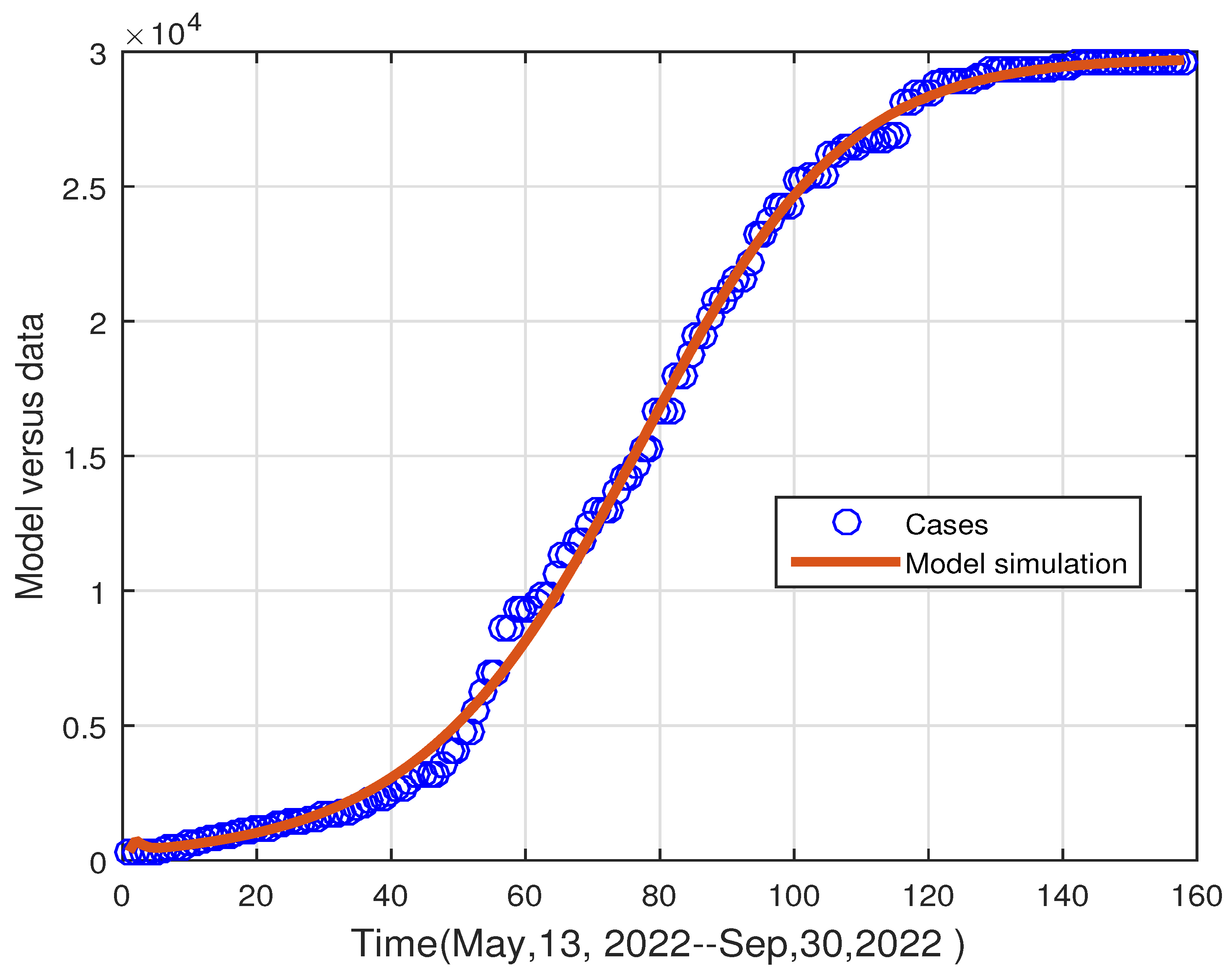
The initial conditions and the total population of Pakistan in 2022 have been considered to be N ( 0 ) = 230,557,367 [39]. The initial conditions have been arranged as follows: S ( 0 ) = 230,255,033, E ( 0 ) = 300,000, A ( 0 ) = 2000 , I ( 0 ) = 334 , and R ( 0 ) = 0 . The specifics of the parameter values acquired during model fitting are shown in Table 1. The numerical values used in Table 1 and the computed basic reproduction number are obtained to be R 0 1.2591 . The result of fitting the data to the model is depicted in Figure 2. The result in Figure 2 shows that the model is well-matched with the data, and hence the parameters obtained are useful in further simulations of the model regarding disease eliminations. It should be noted that we will consider the vaccination model and obtain the graphical results regarding the disease eliminations. In the vaccination model, ω is defined to be the vaccination of healthy people, and its numerical value is considered to be ω = 0.001 . The parameter ψ that measures the vaccine efficacy rate and its numerical value is given by ψ = 0.6 . The immunity loss due to vaccination is given by the parameter θ = 0.01 . It should be noted that no vaccine is 100% effective, and there is a waning of vaccination.

6. Numerical Results

6.1. Numerical scheme

Here, we we shall present the numerical procedure to solve the vaccination fractional order model (12) with the fractional order η ( 0 , 1 ] . We shall use the predictor corrector method of Adams–Moulton type that has already been used in the literature for applications; see [40,41]. System (12) can be rewritten in the form given by:
C D t η w ( t ) = H t , w ( t ) , w ( 0 ) = w 0 , 0 < T < ,
where w = ( S , V , E , A , I , R ) R 6 , H t , w ( t ) is a continuous real-valued vector function that satisfies the Lipschitz condition, while w 0 defines the initial state vector. We have the following when applying the Caputo integral on both sides of Equation (27),
w ( t ) = w 0 + 1 Γ ( η ) 0 t ( t ϖ ) η H ϖ , w ( ϖ ) d ϖ .
We shall explain, in detail, the algorithm by using a uniform grid on [ 0 , T ] with the step-size h = T 0 m and m N . Therefore, the equation given in (28) can follow the following structure when considering the Euler method [42]:
w n + 1 = g 0 + h η Γ ( η + 1 ) j = 0 n ( ( n j + 1 ) η ( n j ) η ) H t j , w ( t j ) , n = 0 , 1 , 2 , , m .
Therefore, we shall use scheme (29) and present the following iterative formulae for our considered system (12):
S n + 1 = S 0 + h η Γ ( η + 1 ) j = 0 η B n , j Π ( β 1 I j + β 2 A j ) S j N j ( ω + μ ) S j + κ R j + θ V j , V n + 1 = V 0 + h η Γ ( η + 1 ) j = 0 η B n , j ω S j ( 1 ψ ) ( β 1 I j + β 2 A j ) V j N j ( θ + μ ) V j , E n + 1 = E 0 + h η Γ ( η + 1 ) j = 0 η B n , j ( β 1 I j + β 2 A j ) S j N j + ( 1 ψ ) ( β 1 I j + β 2 A j ) V j N j ( δ + μ ) E j , A n + 1 = A 0 + h η Γ ( η + 1 ) j = 0 η B n , j q δ E j ( μ + ρ 1 ) A j , I n + 1 = I 0 + h η Γ ( η + 1 ) j = 0 η B n , j ( 1 q ) δ E j ( μ + d + ρ ) I , R n + 1 = R 0 + h η Γ ( η + 1 ) j = 0 η B n , j ρ I j + ρ 1 A j ( κ + μ ) R j ,
where B n , j = ( n j + 1 ) η ( n j ) η . The above scheme shall be considered in the below subsection to present the numerical results graphically.

6.2. Results

We discuss the numerical results of system (3) using the scheme in (30) with the parameter values given in Table 1 and the given initial conditions S ( 0 ) = 230,225,033, V ( 0 ) = 30,000, E ( 0 ) = 300,000, A ( 0 ) = 2000 , I ( 0 ) = 334 , and R ( 0 ) = 0 . We first give a numerical result of model (12) for various values of η in order to demonstrate the effectiveness of the scheme used. It can be observed from Figure 3 that varying η the simulation results converge to their equilibrium point. Hence the solutions regarding the model with the scheme are fine.
Figure 4 represents the impact of the parameter β 2 on the vaccinations and the infected compartments. It can be observed that if contact between asymptomatic people and healthy is minimized, then the number of future cases shall be minimized. It should be noted that asymptomatic individuals do not have clear symptoms, which makes them difficult to identify. If we need to minimize disease spread, then we shall use lockdown, maintain social distancing, and follow other suggestions of the World Health Organization (WHO).
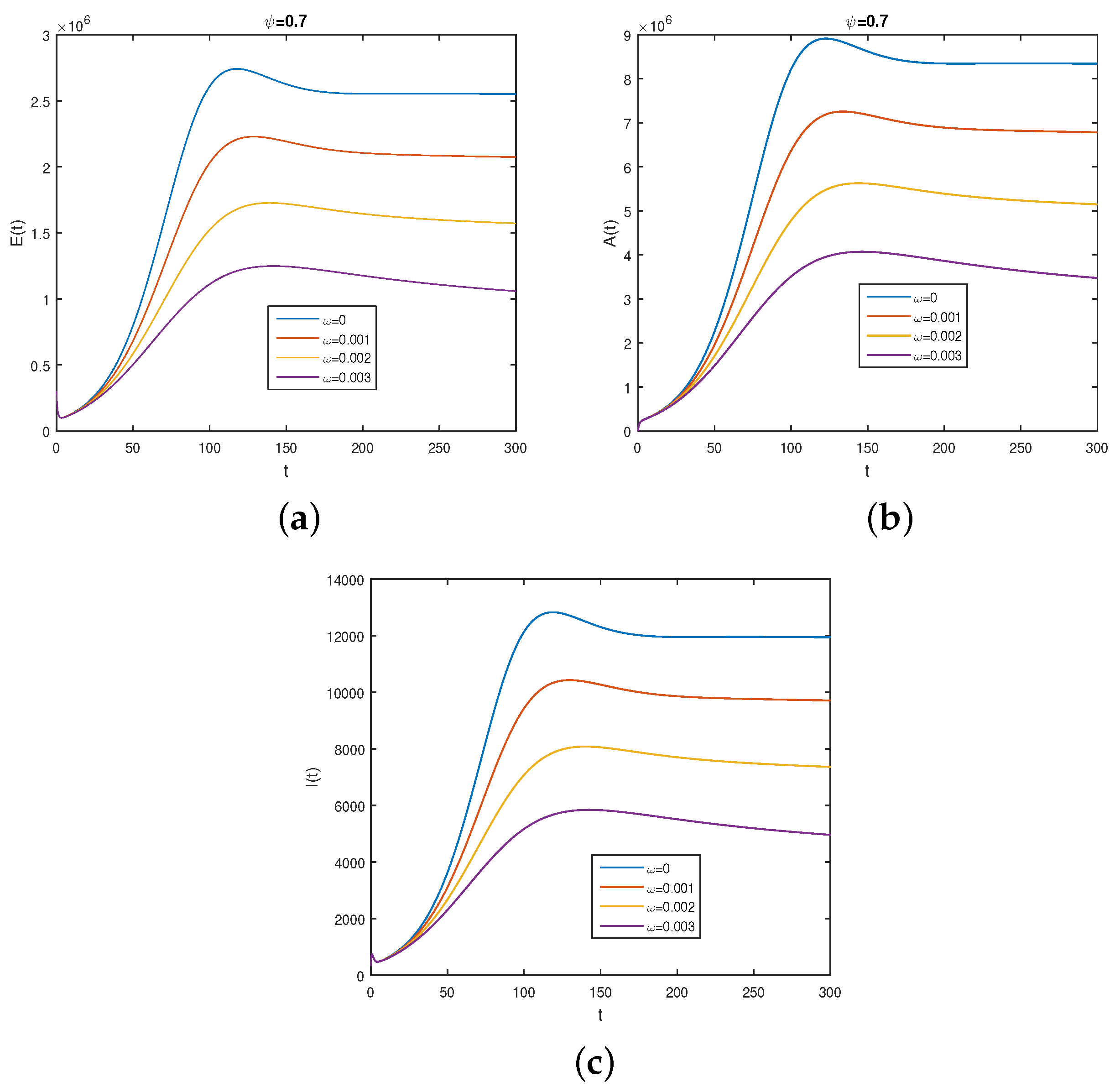
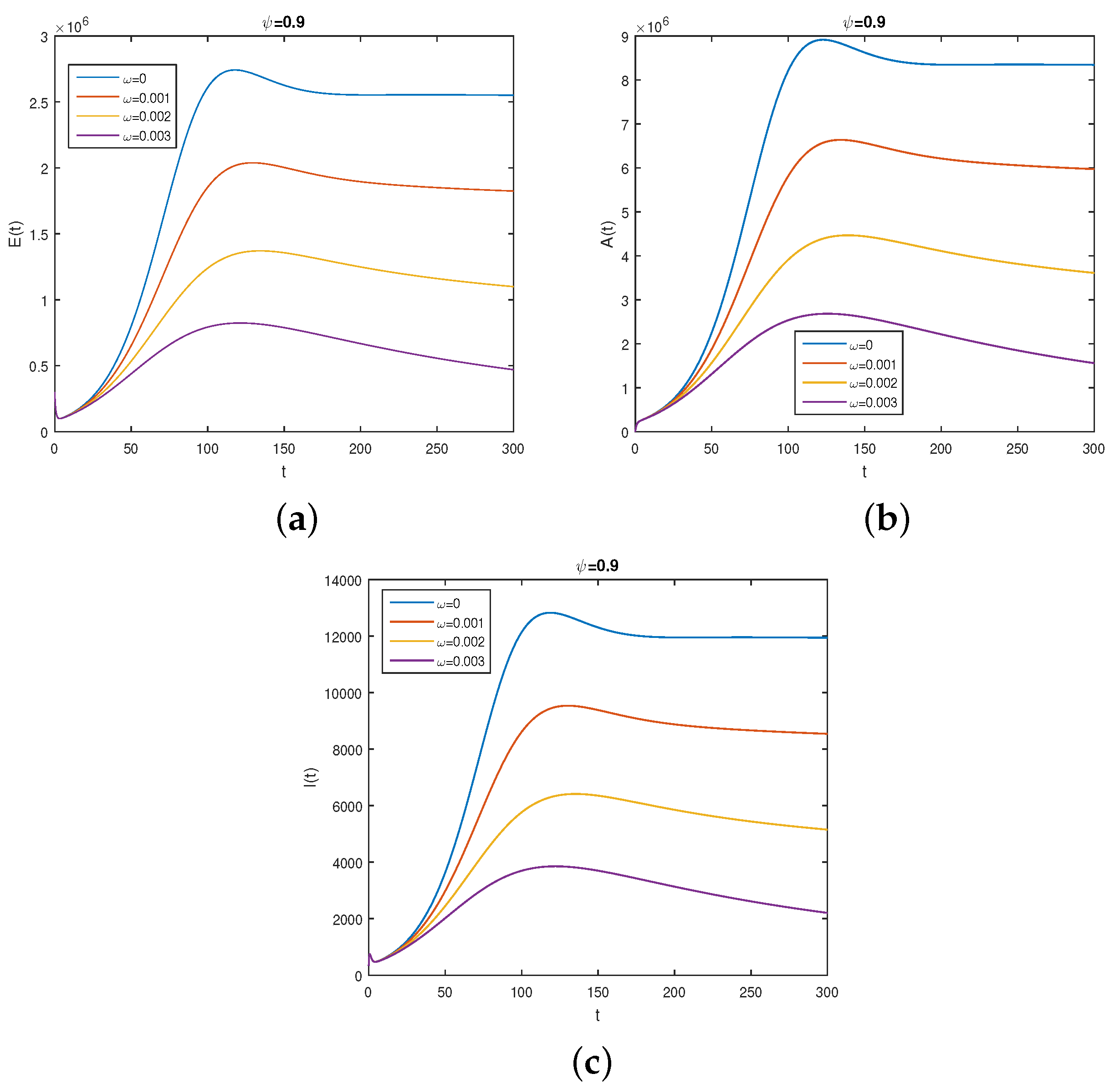
Figure 5, Figure 6 and Figure 7 represent the numerical results of vaccine efficacy. In Figure 5, we consider less efficacy of vaccine ψ = 0.6 and for various values of ω . It can be observed that with vaccination, the cases are decreases. Similarly, improving the vaccine efficacy by using ψ = 0.7 , 0.9 , the number of infected cases decreases, and it can be considered useful. The vaccination efficacy of any vaccine regarding any disease is important to control the infection spread. Regarding the coronavirus vaccine, researchers and scientists are improving the vaccine efficacy rate against the coronavirus infection.
Figure 8 shows the vaccination efficacy rate on the infected populations. It can be noted from the result in Figure 8 that the number of future cases is decreasing with the improvement in the efficacy rate.
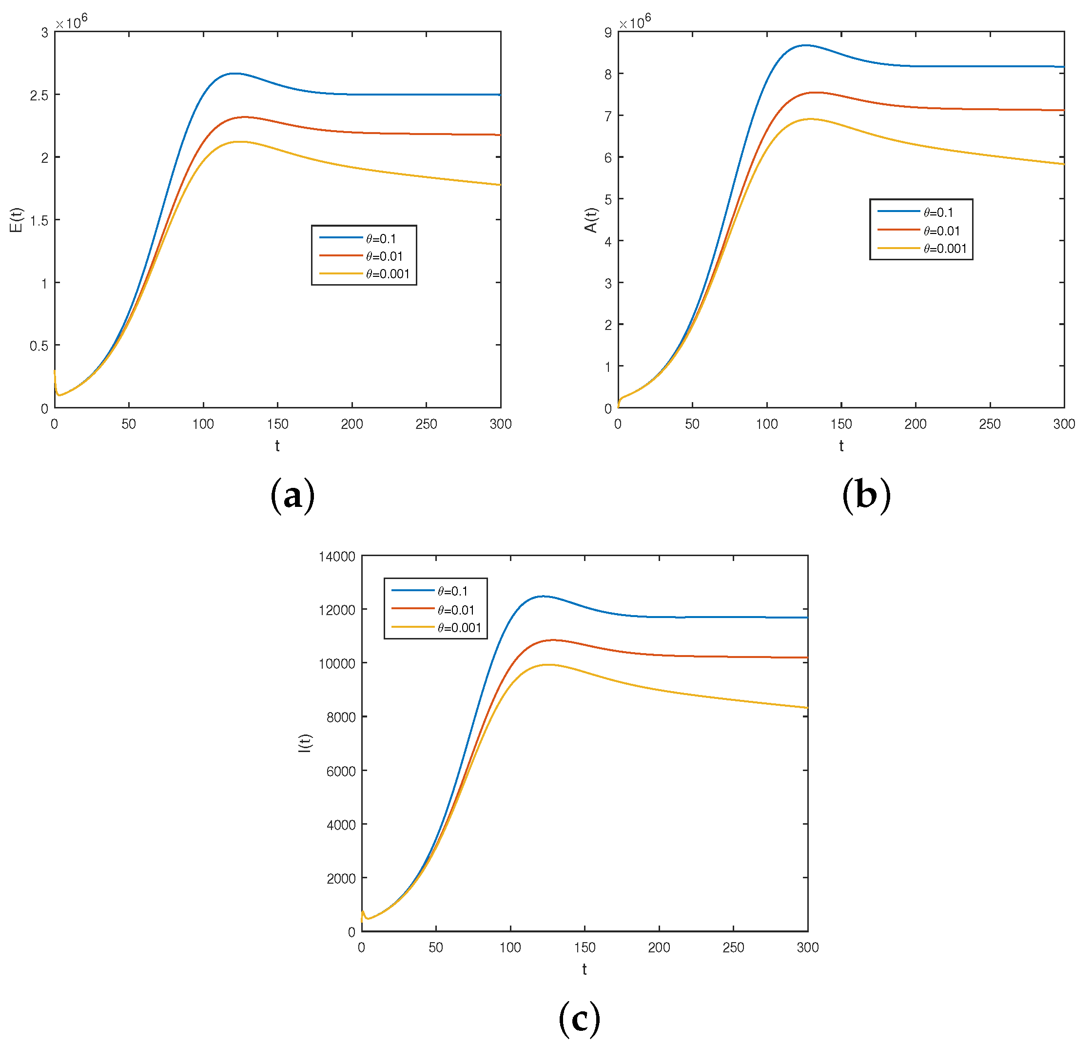
Figure 9 represents the natural immunity loss impact on the infected compartments. With less natural loss of immunity of the individuals, the number of infected people decreases.
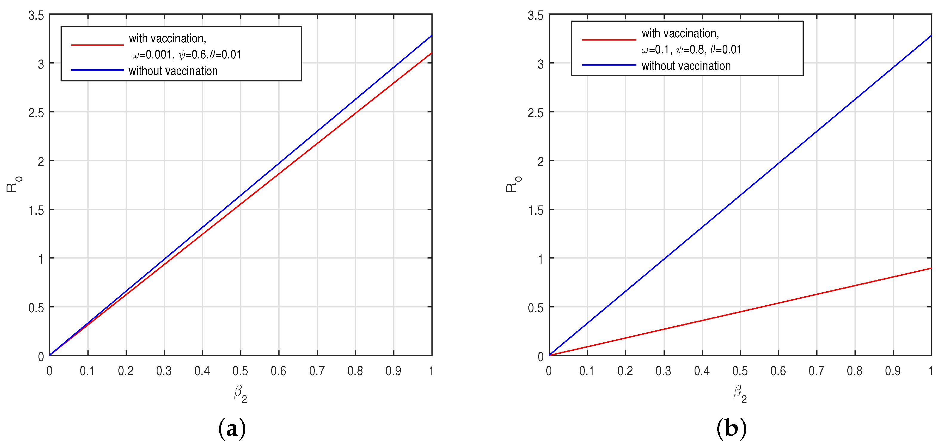
It is well-known that vaccination has great advantages in regard to minimizing the disease spread. The vaccine’s basic reproductive number also what we can call the effective reproductive number minimizes the secondary infection further. We shall compare the result for the case of vaccine and without vaccine reproductive number in Figure 10. It is obvious from the result shown in Figure 10 that the vaccine decreases the basic reproduction number. Further, the vaccine with good efficacy, low waning rate, and expedited vaccination rate can also decrease better the basic reproductive number.

7. Conclusions

In the present paper, we analyzed the dynamics of the coronavirus infection under vaccination impact and immunity decline. We studied the model and presented their local asymptotical stability under the conditions of R 0 v < 1 . We also presented that the vaccination model, under certain conditions, is globally asymptotically stable if R 0 v 1 . The global asymptotical stability of the model is shown for R 0 v > 1 as a special case. We also considered the endemic equilibria and their existence and found that there may be a backward bifurcation under certain conditions. We discussed and added related results for the occurrence of backward bifurcation.
We considered the infected cases of coronavirus infection of the recent wave in the country of Pakistan for the period May–September 2022. We used the nonlinear least square curve fitting method and obtained the realistic values of the model parameters. The numerical value of the basic reproduction number computed for the obtained numerical values in the absence of vaccination is R 0 1.2591 , and with vaccination, the numerical value of the basic reproduction number is R 0 v 1.1907 with less efficacy ψ = 0.6 . Increasing the vaccine efficacy rate up to ψ = 0.8 80% with vaccination rate ω = 0.01 , we have R 0 v 1.1907 . This indicates that our model’s results are reliable and shall be considered for the elimination of infection in the country. The vaccination rate and the efficacy with less immunity decline shall provide reasonable results for the decrease in future cases.
Further, we considered the obtained numerical values of the model parameters and presented the numerical results with a numerical scheme for the Caputo differential equations. Initially, we tested the schemes for various values of the fractional order η on the model equations and found that the model converges to its equilibrium point when varying the value of η . The impact of the model’s parameters that have a great impact on the elimination of infection, in the long run, are plotted graphically. The asymptomatic individuals have been identified to be crucial for the increase in cases. We have obtained the results that the number of cases is increasing rapidly when the asymptomatic rate of infection is increased. One of the reasons is that asymptomatic people greatly contribute to the infected cases due to their lack of visible symptoms, and hence people think they are healthy unless they get tested. Vaccine efficacy has a great role in disease elimination. If the vaccination has a high efficacy rate, then the number of cases shall be minimized, and the further disease cases shall be less. In our numerical results, we found that by increasing the efficacy and vaccine rate, the number of future infected cases decrease. The natural immunity loss also causes an increase in future cases. If there is less natural loss in immunity, then the number of future cases will be decreased. In the future, this work can be extended using new numerical approaches with newly defined fractional operators and a comparison with other numerical methods shall be drawn.

Author Contributions

Conceptualization, T.-C.S., M.H.D., M.A.K. and S.S.A.; Data curation, A.S.A., W.F.A., S.S.A. and T.M.; Formal analysis, T.-C.S., M.A.K., S.S.A., W.F.A. and T.M.; Investigation, T.-C.S., M.H.D., A.S.A., W.F.A., S.S.A. and T.M.; Methodology, T.-C.S., M.A.K. and A.S.A.; Project administration, M.A.K. and S.S.A.; Resources, T.-C.S., M.H.D., M.A.K., W.F.A., S.S.A. and T.M.; Software, M.H.D., W.F.A., M.A.K., S.S.A. and T.M.; Supervision, M.A.K. and A.S.A.; Validation, M.H.D., M.A.K., A.S.A., W.F.A. and T.M.; Visualization, S.S.A.; Writing—original draft, T.-C.S., M.H.D., M.A.K., A.S.A. and T.M.; Writing—review and editing, W.F.A. and T.M. All authors have read and agreed to the published version of the manuscript.

Funding

Princess Nourah bint Abdulrahman University Researchers Supporting Project number (PNURSP2023R 371), Princess Nourah bint Abdulrahman University, Riyadh, Saudi Arabia.

Institutional Review Board Statement

Not applicable.

Informed Consent Statement

Not applicable.

Data Availability Statement

Data are available from corresponding authors on reasonable request.

Acknowledgments

Princess Nourah bint Abdulrahman University Researchers Supporting Project number (PNURSP2023R 371), Princess Nourah bint Abdulrahman University, Riyadh, Saudi Arabia. The authors extend their appreciation to the Deanship of Scientific Research at King Khalid University for funding this work through Large Groups project under grant number RGP.2/314.

Conflicts of Interest

The authors declare no conflict of interest.

References

  1. World/Countries/Pakistan, Total Coronavirus Cases in Pakistan. Available online: https://www.worldometers.info/coronavirus/country/pakistan/ (accessed on 30 November 2022).
  2. Khajanchi, S.; Sarkar, K.; Banerjee, S. Modeling the dynamics of COVID-19 pandemic with implementation of intervention strategies. Eur. Phys. J. Plus 2022, 137, 1–22. [Google Scholar] [CrossRef] [PubMed]
  3. Ullah, M.S.; Higazy, M.; Kabir, K.A. Modeling the epidemic control measures in overcoming COVID-19 outbreaks: A fractional-order derivative approach. Chaos Solitons Fractals 2022, 155, 111636. [Google Scholar] [CrossRef] [PubMed]
  4. Cioffi, A.; Cioffi, F. COVID-19 vaccine: Risk of inequality and failure of public health strategies. Ethics Med. Public Health 2021, 17, 100653. [Google Scholar] [CrossRef] [PubMed]
  5. Zheng, Q.; Wang, X.; Bao, C.; Ji, Y.; Liu, H.; Meng, Q.; Pan, Q. A multi-regional, hierarchical-tier mathematical model of the spread and control of COVID-19 epidemics from epicentre to adjacent regions. Transbound. Emerg. Dis. 2022, 69, 549–558. [Google Scholar] [CrossRef]
  6. Deng, J.; Tang, S.; Shu, H. Joint impacts of media, vaccination and treatment on an epidemic Filippov model with application to COVID-19. J. Theor. Biol. 2021, 523, 110698. [Google Scholar] [CrossRef]
  7. Chen, C.; Chong, N.S. A Filippov model describing the effects of media coverage and quarantine on the spread of human influenza. Math. Biosci. 2018, 296, 98–112. [Google Scholar] [CrossRef]
  8. Acuña-Zegarra, M.A.; Díaz-Infante, S.; Baca-Carrasco, D.; Olmos-Liceaga, D. COVID-19 optimal vaccination policies: A modeling study on efficacy, natural and vaccine-induced immunity responses. Math. Biosci. 2021, 337, 108614. [Google Scholar] [CrossRef]
  9. Omame, A.; Umana, R.; Okuonghae, D.; Inyama, S. Mathematical analysis of a two-sex Human Papillomavirus (HPV) model. Int. J. Biomath. 2018, 11, 1850092. [Google Scholar] [CrossRef]
  10. Elbasha, E.; Podder, C.; Gumel, A. Analyzing the dynamics of an SIRS vaccination model with waning natural and vaccine-induced immunity. Nonlinear Anal. Real World Appl. 2011, 12, 2692–2705. [Google Scholar] [CrossRef]
  11. Doutor, P.; Rodrigues, P.; Soares, M.d.C.; Chalub, F.A. Optimal vaccination strategies and rational behaviour in seasonal epidemics. J. Math. Biol. 2016, 73, 1437–1465. [Google Scholar] [CrossRef] [Green Version]
  12. Laarabi, H.; Rachik, M.; El Kahlaoui, O.; Labriji, E. Optimal vaccination strategies of an SIR epidemic model with a saturated treatment. Univers. J. Appl. Math. 2013, 1, 185–191. [Google Scholar] [CrossRef]
  13. Parsamanesh, M.; Farnoosh, R. On the global stability of the endemic state in an epidemic model with vaccination. Math. Sci. 2018, 12, 313–320. [Google Scholar] [CrossRef]
  14. Parsamanesh, M.; Erfanian, M.; Mehrshad, S. Stability and bifurcations in a discrete-time epidemic model with vaccination and vital dynamics. BMC Bioinform. 2020, 21, 1–15. [Google Scholar] [CrossRef] [PubMed]
  15. Han, X.; Liu, H.; Lin, X.; Wei, Y.; Ming, M. Dynamic Analysis of a VSEIR Model with Vaccination Efficacy and Immune Decline. Adv. Math. Phys. 2022, 2022. [Google Scholar] [CrossRef]
  16. Khan, M.A.; Atangana, A. Modeling the dynamics of novel coronavirus (2019-nCov) with fractional derivative. Alex. Eng. J. 2020, 59, 2379–2389. [Google Scholar] [CrossRef]
  17. Khan, M.A.; Atangana, A.; Alzahrani, E. The dynamics of COVID-19 with quarantined and isolation. Adv. Differ. Equ. 2020, 2020, 1–22. [Google Scholar] [CrossRef]
  18. Oud, M.A.A.; Ali, A.; Alrabaiah, H.; Ullah, S.; Khan, M.A.; Islam, S. A fractional order mathematical model for COVID-19 dynamics with quarantine, isolation, and environmental viral load. Adv. Differ. Equ. 2021, 2021, 1–19. [Google Scholar]
  19. Rihan, F.; Alsakaji, H. Dynamics of a stochastic delay differential model for COVID-19 infection with asymptomatic infected and interacting people: Case study in the UAE. Results Phys. 2021, 28, 104658. [Google Scholar] [CrossRef]
  20. Anggriani, N.; Ndii, M.Z.; Amelia, R.; Suryaningrat, W.; Pratama, M.A.A. A mathematical COVID-19 model considering asymptomatic and symptomatic classes with waning immunity. Alex. Eng. J. 2022, 61, 113–124. [Google Scholar] [CrossRef]
  21. Liu, X.; Ullah, S.; Alshehri, A.; Altanji, M. Mathematical assessment of the dynamics of novel coronavirus infection with treatment: A fractional study. Chaos Solitons Fractals 2021, 153, 111534. [Google Scholar] [CrossRef]
  22. Beigi, A.; Yousefpour, A.; Yasami, A.; Gómez-Aguilar, J.; Bekiros, S.; Jahanshahi, H. Application of reinforcement learning for effective vaccination strategies of coronavirus disease 2019 (COVID-19). Eur. Phys. J. Plus 2021, 136, 1–22. [Google Scholar] [CrossRef] [PubMed]
  23. Martinez-Guerra, R.; Flores-Flores, J.P. An algorithm for the robust estimation of the COVID-19 pandemics population by considering undetected individuals. Appl. Math. Comput. 2021, 405, 126273. [Google Scholar] [PubMed]
  24. Khan, M.A.; Ullah, S.; Kumar, S. A robust study on 2019-nCOV outbreaks through non-singular derivative. Eur. Phys. J. Plus 2021, 136, 1–20. [Google Scholar] [CrossRef] [PubMed]
  25. Khan, M.A.; Atangana, A. Mathematical modeling and analysis of COVID-19: A study of new variant Omicron. Phys. A Stat. Mech. Its Appl. 2022, 599, 127452. [Google Scholar] [CrossRef]
  26. Muniyappan, A.; Sundarappan, B.; Manoharan, P.; Hamdi, M.; Raahemifar, K.; Bourouis, S.; Varadarajan, V. Stability and numerical solutions of second wave mathematical modeling on covid-19 and omicron outbreak strategy of pandemic: Analytical and error analysis of approximate series solutions by using hpm. Mathematics 2022, 10, 343. [Google Scholar] [CrossRef]
  27. Pandey, P.; Gómez-Aguilar, J.; Kaabar, M.K.; Siri, Z.; Abd Allah, A.M. Mathematical modeling of COVID-19 pandemic in India using Caputo-Fabrizio fractional derivative. Comput. Biol. Med. 2022, 145, 105518. [Google Scholar] [CrossRef]
  28. Zhang, C.; Agarwal, R.P.; Bohner, M.; Li, T. Oscillation of second-order nonlinear neutral dynamic equations with noncanonical operators. Bull. Malays. Math. Sci. Soc. 2015, 38, 761–778. [Google Scholar] [CrossRef]
  29. Chen, S.; Zhao, Q.; Ye, Y.; Qu, B. Using IIR filter in fractional order phase lead compensation PIMR-RC for grid-tied inverters. In IEEE Transactions on Industrial Electronics; IEEE: Piscataway, NJ, USA, 2022; pp. 1–10. [Google Scholar] [CrossRef]
  30. Areshi, M.; Seadawy, A.R.; Ali, A.; Alharbi, A.F.; Aljohani, A.F. Analytical Solutions of the Predator–Prey Model with Fractional Derivative Order via Applications of Three Modified Mathematical Methods. Fractal Fract. 2023, 7, 128. [Google Scholar] [CrossRef]
  31. Wu, X.; Wen, S.; Shao, W.; Wang, J. Numerical Investigation of Fractional Step-Down ELS Option. Fractal Fract. 2023, 7, 126. [Google Scholar] [CrossRef]
  32. He, Y.; Wang, Z. Stability analysis and optimal control of a fractional cholera epidemic model. Fractal Fract. 2022, 6, 157. [Google Scholar] [CrossRef]
  33. Baba, I.A.; Humphries, U.W.; Rihan, F.A. Role of Vaccines in Controlling the Spread of COVID-19: A Fractional-Order Model. Vaccines 2023, 11, 145. [Google Scholar] [CrossRef] [PubMed]
  34. Okyere, S.; Ackora-Prah, J. Modeling and analysis of monkeypox disease using fractional derivatives. Results Eng. 2023, 17, 100786. [Google Scholar] [CrossRef] [PubMed]
  35. Kilbas, A.A.; Srivastava, H.M.; Trujillo, J.J. Theory and Applications of Fractional Differential Equations; Elsevier: Amsterdam, The Netherlands, 2006; Volume 204. [Google Scholar]
  36. Odibat, Z.M.; Shawagfeh, N.T. Generalized Taylor’s formula. Appl. Math. Comput. 2007, 186, 286–293. [Google Scholar] [CrossRef]
  37. Van den Driessche, P.; Watmough, J. Reproduction numbers and sub-threshold endemic equilibria for compartmental models of disease transmission. Math. Biosci. 2002, 180, 29–48. [Google Scholar] [CrossRef]
  38. Pakistan Life Expectancy 1950–2022. Available online: https://www.macrotrends.net/countries/PAK/pakistan/life-expectancy (accessed on 5 November 2022).
  39. Pakistan Population. Available online: https://www.worldometers.info/world-population%/pakistan-population/ (accessed on 5 November 2022).
  40. Jajarmi, A.; Baleanu, D. A new fractional analysis on the interaction of HIV with CD4+ T-cells. Chaos Solitons Fractals 2018, 113, 221–229. [Google Scholar] [CrossRef]
  41. Qureshi, S.; Bonyah, E.; Shaikh, A.A. Classical and contemporary fractional operators for modeling diarrhea transmission dynamics under real statistical data. Phys. A Stat. Mech. Its Appl. 2019, 535, 122496. [Google Scholar] [CrossRef]
  42. Li, C.; Zeng, F. Numerical Methods for Fractional Calculus; Chapman and Hall/CRC: Boca Raton, FL, USA, 2015. [Google Scholar]
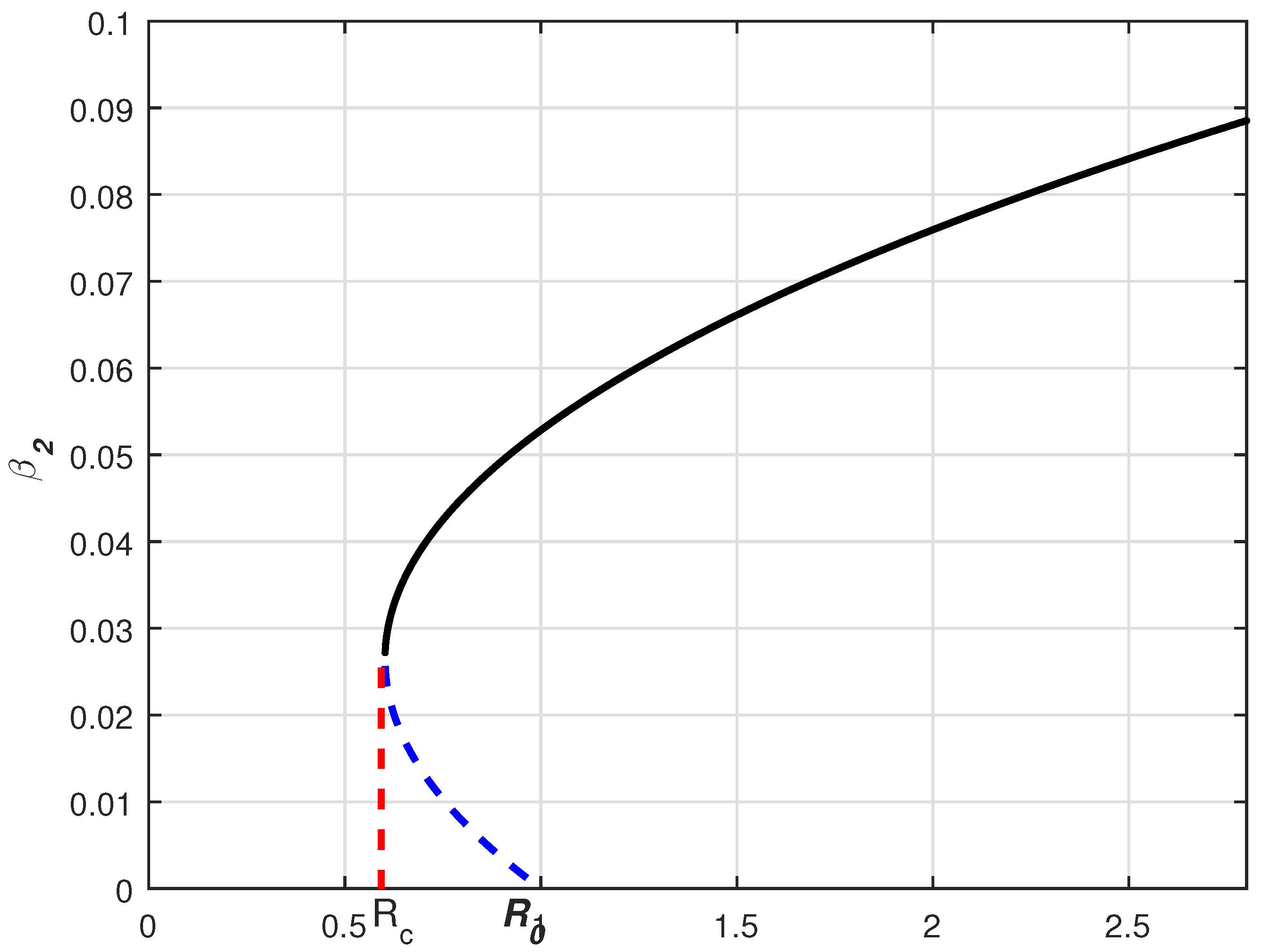
Figure 1. Backward bifurcation plot for model (3).
Fractalfract 07 00234 g001
Figure 2. Data fitting to the model using the parameters given in Table 1.
Fractalfract 07 00234 g002
Figure 3. Simulation of model (3) under various values of the fractional order η . Subfigures (af) describes the dynamics of susceptible, vaccinated, exposed, asymptomatic, symptomatic, and recovered individuals respectively.
Fractalfract 07 00234 g003
Figure 4. Simulation of the model components for different values of δ and η = 0.95 . Subfigures (ad) describe the dynamics of vaccinated, exposed, asymptomatic, and symptomatic individuals respectively.
Fractalfract 07 00234 g004
Figure 5. Impact of the vaccination rate on the components of the system for different values of ω and less efficacy, ψ = 0.6 and η = 0.95 . Subfigures (ad) describe the dynamics of vaccinated, exposed, asymptomatic, and symptomatic individuals respectively.
Fractalfract 07 00234 g005
Figure 6. Impact of the vaccination rate on the components of the system for different values of ω and efficacy, ψ = 0.7 and η = 0.95 . Subfigures (ac) describes the dynamics of exposed, asymptomatic, and symptomatic individuals respectively.
Fractalfract 07 00234 g006
Figure 7. Impact of the vaccination rate on the model components for different values of ω and more effective efficacy, ψ = 0.9 and η = 0.95 . Subfigures (ac) describe the dynamics of exposed, asymptomatic, and symptomatic individuals respectively.
Fractalfract 07 00234 g007
Figure 8. Vaccination efficacy rate on infected compartment ψ with η = 0.95 . Subfigures (ac) describes the dynamics of exposed, asymptomatic, and symptomatic individuals respectively.
Fractalfract 07 00234 g008
Figure 9. Impact of the natural loss of immunity on infected compartments, θ with η = 0.95 . Subfigures (ac) describes the dynamics of exposed, asymptomatic, and symptomatic individuals respectively.
Fractalfract 07 00234 g009
Figure 10. Comparison of the basic reproduction for various values of ω , ψ , and θ for with and without vaccine cases. Subfigures (a,b) describe the comparison of the basic reproduction numbers for various values of ω = 0.01 , ψ = 0.6 , θ = 0.01 and ω = 0.1 , ψ = 0.8 , θ = 0.01 , respectively.
Fractalfract 07 00234 g010
Table 1. Parameter details.
SymbolDefinitionsNumeric ValueRef
Π Birth rate μ × N ( 0 ) Estimated
μ Natural mortality rate 1 67.7 × 365 [38]
β 1 Contact between healthy and sick people0.8983Fitted
β 2 Contact between healthy and asymptomatic people0.3827Fitted
κ Natural immunity loss0.3129Fitted
δ Incubation time period0.9982Fitted
qThe proportion joins class A0.9931Fitted
1 q The proportion joins class I0.0069Fitted
ρ 1 Recovery rate of asymptomatic people0.3028Fitted
ρ Recovery of symptomatic people0.7926Fitted
dDisease death rate of symptomatic people0.6784Fitted
Disclaimer/Publisher’s Note: The statements, opinions and data contained in all publications are solely those of the individual author(s) and contributor(s) and not of MDPI and/or the editor(s). MDPI and/or the editor(s) disclaim responsibility for any injury to people or property resulting from any ideas, methods, instructions or products referred to in the content.