

An Application of the Homotopy Analysis Method for the Time- or Space-Fractional Heat Equation


Abstract
1. Introduction
2. Formulation of the Problems
3. The Homotopy Analysis Method
4. Examples
4.1. Example 1
4.2. Example 2
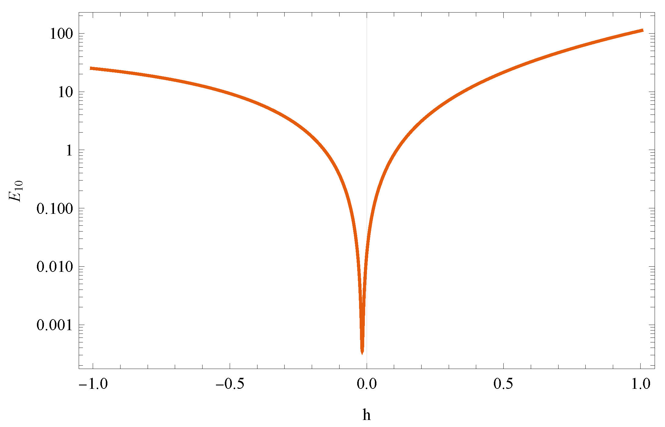
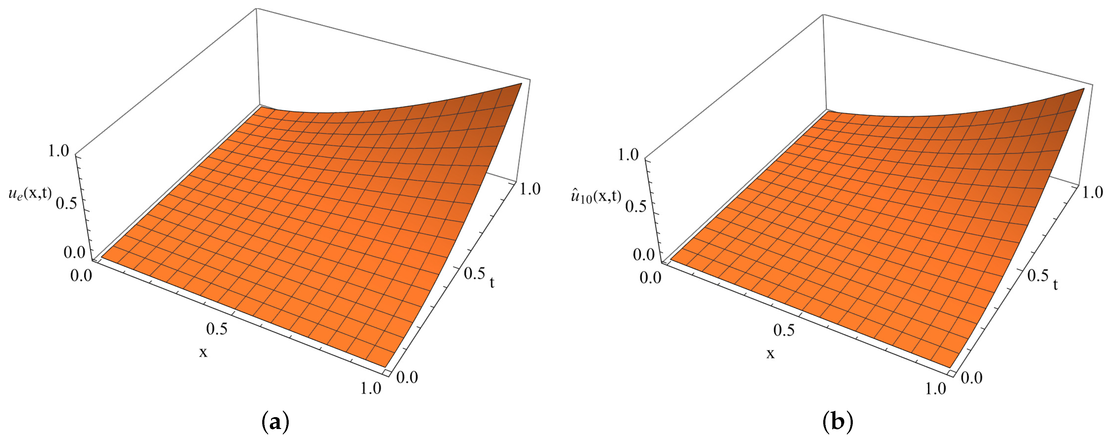
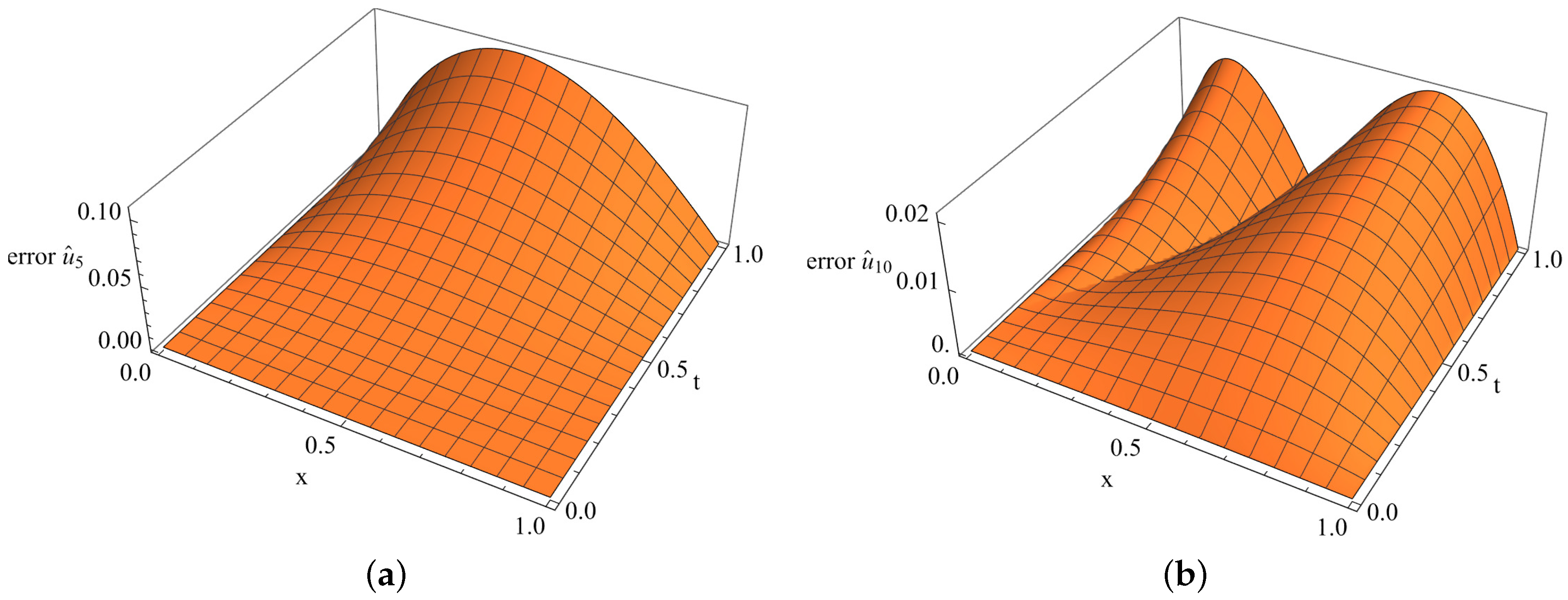
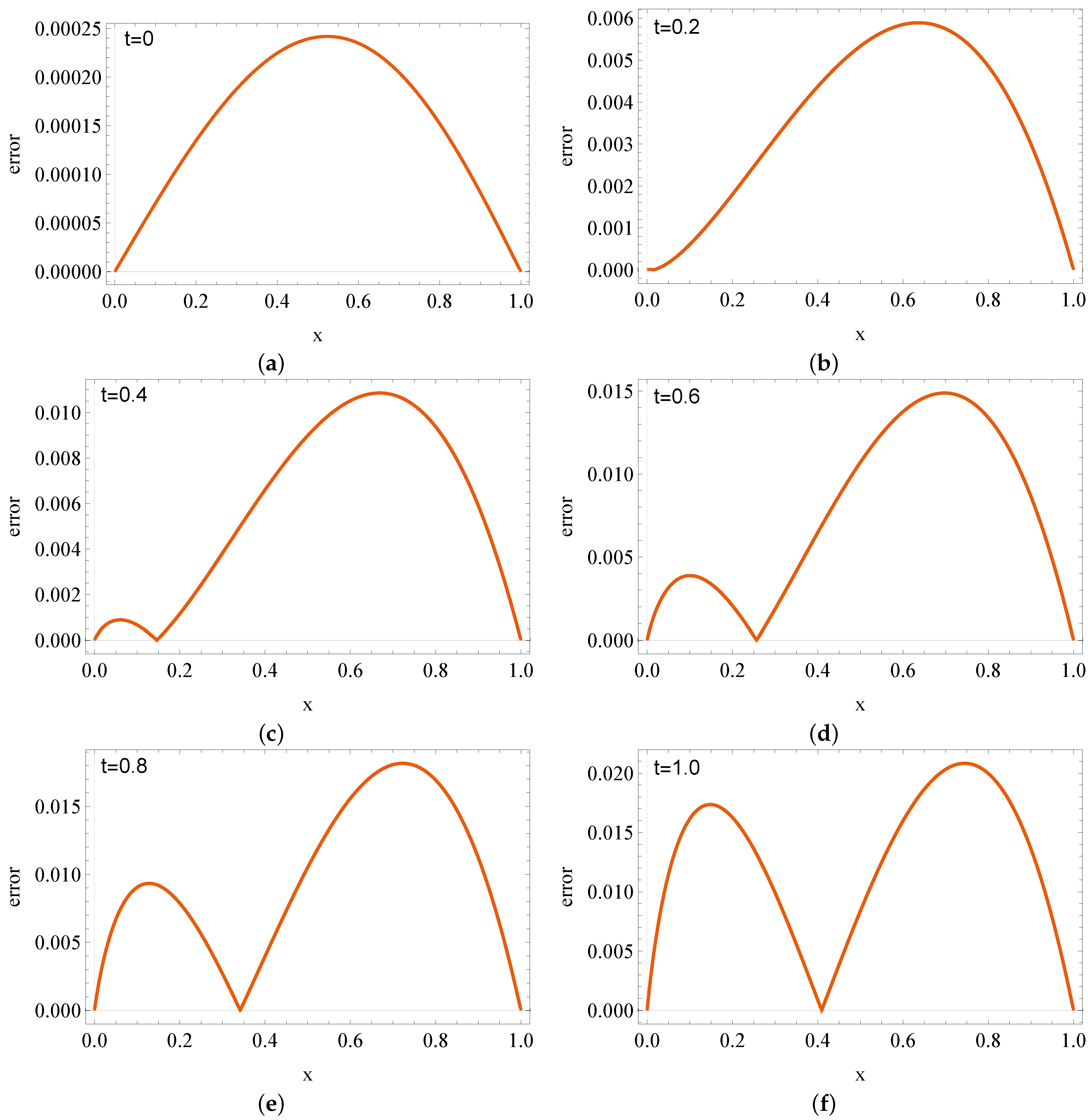
4.3. Example 3
5. Conclusions
Author Contributions
Funding
Data Availability Statement
Acknowledgments
Conflicts of Interest
References
- Dou, F.; Hon, Y. Numerical computation for backward time-fractional diffusion equation. Eng. Anal. Bound. Elem. 2014, 40, 138–146. [Google Scholar] [CrossRef]
- Voller, V. Anomalous heat transfer: Examples, fundamentals, and fractional calculus models. Adv. Heat Transf. 2018, 50, 333–380. [Google Scholar] [CrossRef]
- Błasik, M. A numerical method for the solution of the two-phase fractional Lamé-Clapeyron-Stefan problem. Mathematics 2020, 8, 2157. [Google Scholar] [CrossRef]
- Chmielowska, A.; Słota, D. Fractional Stefan Problem Solving by the Alternating Phase Truncation Method. Symmetry 2022, 14, 2287. [Google Scholar] [CrossRef]
- Zhuang, Q.; Yu, B.; Jiang, X. An inverse problem of parameter estimation for time-fractional heat conduction in a composite medium using carbon–carbon experimental data. Physica B 2015, 456, 9–15. [Google Scholar] [CrossRef]
- Brociek, R.; Słota, D.; Król, M.; Matula, G.; Kwaśny, W. Comparison of mathematical models with fractional derivative for the heat conduction inverse problem based on the measurements of temperature in porous aluminum. Int. J. Heat Mass Transfer 2019, 143, 118440. [Google Scholar] [CrossRef]
- Garshasbi, M.; Sanaei, F. A variable time-step method for a space fractional diffusion moving boundary problem: An application to planar drug release devices. Int. J. Numer. Model. 2021, 34, e2852. [Google Scholar] [CrossRef]
- Rajeev; Kushwaha, M.; Kumar, A. An approximate solution to a moving boundary problem with space-time fractional derivative in fluvio-deltaic sedimentation process. Ain Shames Eng. J. 2013, 4, 889–895. [Google Scholar] [CrossRef]
- Brociek, R.; Słota, D.; Król, M.; Matula, G.; Kwaśny, W. Modeling of Heat Distribution in Porous Aluminum Using Fractional Differential Equation. Fractal Fract. 2017, 1, 17. [Google Scholar] [CrossRef]
- Liao, S. Homotopy analysis method: A new analytic method for nonlinear problems. Appl. Math. Mech. Engl. Ed. 1998, 19, 957–962. [Google Scholar] [CrossRef]
- Liao, S. Beyond Perturbation: Introduction to the Homotopy Analysis Method; Chapman and Hall–CRC Press: Boca Raton, FL, USA, 2003. [Google Scholar]
- Liao, S. Homotopy Analysis Method in Nonlinear Differential Equations; Springer/Higher Education Press: Berlin/Heidelberg, Germany, 2012. [Google Scholar]
- Chauhan, D.; Agrawal, R.; Rastogi, P. Magnetohydrodynamic slip flow and heat transfer in a porous medium over a stretching cylinder: Homotopy analysis method. Numer. Heat Transf. A 2012, 62, 136–157. [Google Scholar] [CrossRef]
- Van Gorder, R. Control of error in the homotopy analysis of semi-linear elliptic boundary value problems. Numer. Algor. 2012, 61, 613–629. [Google Scholar] [CrossRef]
- Hetmaniok, E.; Słota, D.; Wituła, R.; Zielonka, A. An Analytical Method for Solving the Two-Phase Inverse Stefan Problem. Bull. Pol. Acad. Sci. Tech. Sci. 2015, 63, 583–590. [Google Scholar] [CrossRef]
- Abbasbandy, S.; Shivanian, E. A new analytical technique to solve Fredholm’s integral equations. Numer. Algor. 2011, 56, 27–43. [Google Scholar] [CrossRef]
- Hetmaniok, E.; Słota, D.; Trawiński, T.; Wituła, R. Usage of the Homotopy Analysis Method for Solving the Nonlinear and Linear Integral Equations of the Second Kind. Numer. Algor. 2014, 67, 163–185. [Google Scholar] [CrossRef]
- Hetmaniok, E.; Nowak, I.; Słota, D.; Wituła, R. Convergence and Error Estimation of Homotopy Analysis Method for Some Type of Nonlinear and Linear Integral Equations. J. Numer. Math. 2015, 23, 331–344. [Google Scholar] [CrossRef]
- Mohamed, M.; Gepreel, K.; Alharthi, M.; Alotabi, R. Homotopy analysis transform method for integro-differential equations. Gen. Math. Notes 2016, 32, 32–48. [Google Scholar]
- Alipouru, M.; Vali, M.; Borzabadi, A. A direct approach for approximate optimal control of integro-differential equations based on homotopy analysis and parametrization method. IMA J. Math. Control. Inform. 2017, 34, 611–630. [Google Scholar] [CrossRef]
- Słota, D.; Hetmaniok, E.; Wituła, R.; Gromysz, K.; Trawiński, T. Homotopy approach for integrodifferential equations. Mathematics 2019, 7, 904. [Google Scholar] [CrossRef]
- Van Gorder, R.; Vajravelu, K. On the selection of auxiliary functions, operators, and convergence control parameters in the application of the homotopy analysis method to nonlinear differential equations: A general approach. Commun. Nonlinear Sci. Numer. Simulat. 2009, 14, 4078–4089. [Google Scholar] [CrossRef]
- Odibat, Z. A study on the convergence of homotopy analysis method. Appl. Math. Comput. 2010, 217, 782–789. [Google Scholar] [CrossRef]
- Abdulaziz, O.; Bataineh, A.; Hashim, I. On convergence of homotopy analysis method and its modification for fractional modified KdV equations. J. Appl. Math. Comput. 2010, 33, 61–81. [Google Scholar] [CrossRef]
- Saad, K.; AL-Shareef, E.; Alomari, A.; Baleanu, D.; Gómez-Aguilar, J. On exact solutions for time-fractional Korteweg-de Vries and Korteweg-de Vries-Burger’s equations using homotopy analysis transform method. Chin. J. Phys. 2020, 63, 149–162. [Google Scholar] [CrossRef]
- Xu, H.; Cang, J. Analysis of a time fractional wave-like equation with the homotopy analysis method. Phys. Lett. A 2008, 372, 1250–1255. [Google Scholar] [CrossRef]
- Xu, H.; Liao, S.J.; You, X.C. Analysis of nonlinear fractional partial differential equations with the homotopy analysis method. Commun. Nonlinear Sci. Numer. Simul. 2009, 14, 1152–1156. [Google Scholar] [CrossRef]
- Jafari, H.; Seifi, S. Homotopy analysis method for solving linear and nonlinear fractional diffusion-wave equation. Commun. Nonlinear Sci. Numer. Simul. 2009, 14, 2006–2012. [Google Scholar] [CrossRef]
- Sarwar, S.; Alkhalaf, S.; Iqbal, S.; Zahid, M. A note on optimal homotopy asymptotic method for the solutions of fractional order heat- and wave-like partial differential equations. Comput. Math. Appl. 2015, 70, 942–953. [Google Scholar] [CrossRef]
- Odibat, Z.; Baleanu, D. A linearization-based approach of homotopy analysis method for non-linear time-fractional parabolic PDEs. Math. Methods Appl. Sci. 2019, 42, 7222–7232. [Google Scholar] [CrossRef]
- Słota, D.; Chmielowska, A.; Brociek, R.; Szczygieł, M. Application of the Homotopy Method for Fractional Inverse Stefan Problem. Energies 2020, 13, 5474. [Google Scholar] [CrossRef]
- Arafa, A.; Rida, S.; Mohamed, H. Approximate analytical solutions of Schnakenberg systems by homotopy analysis method. Appl. Math. Model. 2012, 36, 4789–4796. [Google Scholar] [CrossRef]
- Yépez-Martínez, H.; Gómez-Aguilar, J. A new modified definition of Caputo-Fabrizio fractional-order derivative and their applications to the Multi Step Homotopy Analysis Method (MHAM). J. Comput. Appl. Math. 2019, 346, 247–260. [Google Scholar] [CrossRef]
- Shanker Dubey, R.; Goswami, P. Analytical solution of the nonlinear diffusion equation. Eur. Phys. J. Plus 2018, 133, 183. [Google Scholar] [CrossRef]
- Alqahtani, O. Analytical solution of non-linear fractional diffusion equation. Adv. Diff. Eqs. 2021, 2021, 327. [Google Scholar] [CrossRef]
- Odibat, Z. On the optimal selection of the linear operator and the initial approximation in the application of the homotopy analysis method to nonlinear fractional differential equations. Appl. Numer. Math. 2019, 137, 203–212. [Google Scholar] [CrossRef]
- Zhang, X.; Wei, L.; Tang, B.; He, Y. Homotopy analysis method for space-time fractional differential equations. Int. J. Numer. Methods Heat Fluid Flow 2013, 23, 1063–1075. [Google Scholar] [CrossRef]
- Rajaraman, R.; Hariharan, G. Liao’s method for a few space and time fractional reaction-diffusion equations arising in engineering. Int. J. Eng. Technol. 2013, 2013, 3077–3091. [Google Scholar]
- Qu, H.; She, Z.; Liu, X. Homotopy analysis method for three types of fractional partial differential equations. Complexity 2020, 2020, 7232907. [Google Scholar] [CrossRef]
- Povstenko, Y. Fractional Thermoelasticity; Springer: Cham, Switzerland, 2015. [Google Scholar]
- Chen, W.; Sun, H.; Li, X. Fractional Derivative Modeling in Mechanics and Engineering; Science Press: Beijing, China; Springer: Singapore, 2022. [Google Scholar]
- Podlubny, I. Fractional Differential Equations; Academic Press: San Diego, CA, USA, 1999. [Google Scholar]


Disclaimer/Publisher’s Note: The statements, opinions and data contained in all publications are solely those of the individual author(s) and contributor(s) and not of MDPI and/or the editor(s). MDPI and/or the editor(s) disclaim responsibility for any injury to people or property resulting from any ideas, methods, instructions or products referred to in the content. |
© 2023 by the authors. Licensee MDPI, Basel, Switzerland. This article is an open access article distributed under the terms and conditions of the Creative Commons Attribution (CC BY) license (https://creativecommons.org/licenses/by/4.0/).
Share and Cite
Brociek, R.; Wajda, A.; Błasik, M.; Słota, D. An Application of the Homotopy Analysis Method for the Time- or Space-Fractional Heat Equation. Fractal Fract. 2023, 7, 224. https://doi.org/10.3390/fractalfract7030224
Brociek R, Wajda A, Błasik M, Słota D. An Application of the Homotopy Analysis Method for the Time- or Space-Fractional Heat Equation. Fractal and Fractional. 2023; 7(3):224. https://doi.org/10.3390/fractalfract7030224
Chicago/Turabian StyleBrociek, Rafał, Agata Wajda, Marek Błasik, and Damian Słota. 2023. "An Application of the Homotopy Analysis Method for the Time- or Space-Fractional Heat Equation" Fractal and Fractional 7, no. 3: 224. https://doi.org/10.3390/fractalfract7030224
APA StyleBrociek, R., Wajda, A., Błasik, M., & Słota, D. (2023). An Application of the Homotopy Analysis Method for the Time- or Space-Fractional Heat Equation. Fractal and Fractional, 7(3), 224. https://doi.org/10.3390/fractalfract7030224