Article

From Stochastic to Rough Volatility: A New Deep Learning Perspective on Hedging

Antai College of Economics and Management, Shanghai Jiao Tong University, Shanghai 200030, China
*
Author to whom correspondence should be addressed.
Fractal Fract. 2023, 7(3), 225; https://doi.org/10.3390/fractalfract7030225
Submission received: 7 December 2022 / Revised: 17 February 2023 / Accepted: 24 February 2023 / Published: 2 March 2023

Abstract

:
The Black–Scholes model assumes that volatility is constant, and the Heston model assumes that volatility is stochastic, while the rough Bergomi (rBergomi) model, which allows rough volatility, can perform better with high-frequency data. However, classical calibration and hedging techniques are difficult to apply under the rBergomi model due to the high cost caused by its non-Markovianity. This paper proposes a gated recurrent unit neural network (GRU-NN) architecture for hedging with different-regularity volatility. One advantage is that the gating network signals embedded in our architecture can control how the present input and previous memory update the current activation. These gates are updated adaptively in the learning process and thus outperform conventional deep learning techniques in a non-Markovian environment. Our numerical results also prove that the rBergomi model outperforms the other two models in hedging.

1. Introduction

1.1. Motivation

A classical problem in the area of mathematical finance is how to hedge the risk from selling a contingent claim. Option pricing models with different assumed volatility processes have been proposed for this hedging problem. The authors of [1] presented a well-known option pricing formula where the stock price follows a geometric Brownian motion (GBM) and the volatility is a constant. Based on the no-arbitrage arguments, a partial differential equation (PDE) can be derived for option pricing using the Black–Scholes (BS) formula. This PDE can be easily solved and has a closed-form solution. Moreover, the solution’s simplicity and independence of investors’ expectations about the future asset returns have caused it to gain acceptance among practitioners. However, it is observed that the implied volatility (IV) varies across moneyness and maturities, exhibiting the famous IV smile and the at-the-money (ATM) skew, which contradict the constant assumption in the BS model.
In the past three decades, we have witnessed that a number of stochastic volatility (SV) models constantly emerge to justify the IV smile for the BS model, such as the Hull–White model [2], the arithmetic Ornstein–Uhlenbeck model [3], the Bergomi model [4,5] and the Heston model [6]. Among these, ref. [6] derived a closed-form solution for option pricing under stochastic volatility, which has been used for a long time. Then, ref. [7] modified the assumption in the BS model using Bayesian learning and found that it can generate biases similar to those observed in markets. More recently, from a time series analysis of volatility using high-frequency data, Gatheral, Jaisson, and Rosenbaum [8] showed that log-volatility basically behaves as a fractional Brownian motion (fBm) with the Hurst parameter (or exponent) H 0.1 , and proposed the rough fractional stochastic volatility (RFSV) model. Besides its outstanding consistency with the financial market data, the RFSV model also has a quantitative market microstructure foundation based on the modelling of order flow using the Hawkes processes (see [9,10,11]).
Bayer, Friz and Gatheral [12] went a step further and proposed a simple case of the RFSV model: the rough Bergomi (rBergomi) model. With fewer parameters, the rBergomi model can fit the market data significantly better than conventional Markovian stochastic volatility models. Remarkably, the rBergomi model can generate the power-law ATM skew. This term structure is more similar to the market data compared with the exponential-law ATM skew generated by the famous Bergomi model, and this is discussed in [13].

1.2. Aim of This Paper

The primary goal of this paper is to analyze the implications under volatilities with different regularities for option hedging purposes. Two critical issues related to the rBergomi model’s application in equity markets are calibration and hedging. Meanwhile, deep learning techniques are increasingly important in financial model applications. Pioneered by [14], multiple papers have aimed to calibrate rough volatility models through deep learning techniques, e.g., [15,16,17]. In the calibration part of this paper, we adopt the calibration method from [15], in which they proposed a different two-step method solely using deep learning for the pricing map (from model parameters to prices or IV), rather than directly calibrating the model parameters as a function of observed market data. We give a detailed illustration of this approach in Section 3.1 and give its experimental performance under the S&P/FTSE market data, which is implemented in PYTHON using TensorFlow.
Hedging portfolios of derivatives is another critical issue in the financial securities industry. We summarize some pioneering literature here. Ref. [18] implemented a learning model in long-term memory (LSTM) recurrent structures with reinforcement learning to create successful strategies for agents. Jiang, Xu and Liang [19] presented a financial-model-free reinforcement learning framework to provide a deep machine learning solution to portfolio management. Buehler, Gonon, Teichmann and Wood [20] presented a framework for hedging a portfolio of derivatives under the Heston model in the presence of market frictions using a deep reinforcement method. However, those frameworks either used the Q-learning technique or the Markovian volatility models. In this paper, we propose a gated recurrent unit neural network (GRU-NN) architecture for hedging under volatility with different regularities (e.g., rough, stochastic, and constant). Through the comparison of several characteristics, we can conclude that the general hedging performance of the rough Bergomi model outperforms the others, and these findings have important implications for risk management.

1.3. Main Findings

Building upon the ideas from [20], Horvath, Teichmann and Zuric [21] investigated deep hedging performance under training paths exceeding the finite-dimensional Markovian setup, in which they modified the original recurrent network architecture and proposed a fully recurrent network architecture. Here, we go a step further; we propose the GRU-NN architecture for the portfolio selection in Section 3.2 because it is more suitable for capturing the non-Markovianity of the rBergomi model. The parameters H , η , ρ , V 0 are calibrated in Section 3.1. The memory cells in the GRU-NN can model non-Markovian effects very well and thus make this method particularly attractive from the deep learning perspective.

1.4. Contributions of This Paper

Our main technical contributions lie in obtaining the deep hedging performance under volatility models with different regularities, and comparing them with multiple characteristics. We also demonstrate the effectiveness of the GRU-NN. The data used are daily prices of the S&P 500 and FTSE 100 for the period from 31 December 2021 to 15 December 2023, and from 21 January 2022 to 15 December 2023, respectively.
The remainder of this paper is structured as follows. In Section 2, we recall the setup of the rBergomi model and the exponential utility indifference pricing for hedging used in [12,21]. In Section 3.1, we illustrate the architecture of the fully-connected neural networks combined with the LM algorithm and give the calibrated parameters. The main idea is discussed in Section 3.2, where we introduce our GRU-NN architecture using the entropic risk measure with those deep calibrated parameters and give the deep hedging performance. The procedure and the validation results are presented in Section 4. The conclusions are drawn in Section 5.

2. Setup and Notation

2.1. The Stochastic Volatility Model

Assumptions about the underlying asset price dynamics are the essential qualities of option pricing models. Because plenty of empirical studies document the excess kurtosis of financial asset returns’ distributions and their conditional heteroscedasticity, some stochastic volatility models have emerged to justify the volatility smile and permit us to explain its features. Among them, ref. [6] derived a closed-form solution for option pricing in a unique stochastic volatility environment.
Definition 1.
The stochastic volatility model is a two-state model with two sources of risk. Here, we give its representation in the probability space ( Ω , F , P ) as follows. The filtration F = { F t } 0 t T satisfies the ordinary conditions and supports two Brownian motions B t , W t .
d S t d σ t = μ S t μ 2 ( t , S t , σ t ) d t + σ t S t 0 0 σ 2 , 2 ( t , S t , σ t ) d B t d W t ,
where S t is the price of the underlying asset at time t and d B t d W t = ρ d t .
Definition 2.
In [6], an Ornstein–Uhlenbeck (OU) process was suggested for the volatility process. It leads to a square-root process for the instantaneous variance V t = σ t 2 by Itô’s lemma. The state diffusion process in ( Ω , F , P ) then becomes
d S t d V t = μ S t κ ( θ V t ) d t + V t S t 0 0 σ v V t d B t d W t .
Here, we characterize it by the following risk-neutral  ( Ω , F , Q ) dynamics
d S t S t = r d t + V t S d B t , d V t = κ ( θ V t ) d t + σ v V t d W t ,
with d B t d W t = ρ d t , where r is the risk-free rate. The notations in the Heston model are given as follows:
  • κ denotes the variance mean-reversion speed.
  • θ denotes the long-term variance.
  • σ v denotes the volatility of the variance process.
  • V 0 denotes the initial variance.
  • ρ denotes the correlation coefficient of the two correlated Wiener processes B t , W t .
The Heston model considers the leverage and clustering effect, which allows the volatility to be stochastic (Hurst parameter H = 1 / 2 ) and accounts for non-normally distributed asset returns. Empirical studies show that the Heston model markedly outperforms the BS model in nearly all combinations of moneyness and maturity scenarios except when the option is soon to expire; see, for example, [22].

2.2. The Rough Volatility Model

In terms of regularity, the volatility in these models is either very smooth or with a smoothness similar to that of a Brownian motion. To allow for a broader range of smoothness, we can consider the fractional Brownian motion in volatility modelling. This current paper focuses on the rBergomi model under the measure Q , as do [12,23], which can fit short maturities very well. The rBergomi model is defined as below.
Definition 3.
Under the pricing measure Q , the state diffusion process becomes
d S t S t = V t d B t , V t = ξ 0 ( t ) exp η 2 α + 1 0 t ( t s ) α d W s η 2 2 t 2 α + 1 ,
where α = H 1 2 , on the given space Ω , F , ( F t ) t 0 , Q . The driving random variables B t and W t have the relationship of d B t d W t = ρ d t .
Without losing generality, we set the observed initial forward variance curve ξ 0 ( t ) at inception as a constant and denote it as V 0 . Hence, the notations in the rBergomi model are given below.
  • H = α + 0.5 is the Hurst parameter, which takes a value around 0.1 .
  • η is the level of the volatility in the variance.
  • V 0 is the initial variance.
  • ρ denotes the correlation coefficient of the Wiener processes d B t , d W t .
The process
V t : = 0 t ( t u ) α d W u
in the volatility V t is a centred Gaussian process with the following covariance structure:
E ( V t V s ) = s 2 H 0 t t 2 u α ( 1 u ) α d u , for any s , t [ 0 , 1 ] ,
and the quadratic variation
[ V ] t = t 2 H 2 H , for t 0 .
As for the simulation of the rBergomi model, Bayer, Friz and Gatheral presented the Cholesky method for simulation in [12]. Because the Volterra process V is a truncated Brownian semi-stationary (tBSS) process, we use the hybrid scheme proposed in [24] instead to speed up the process for calibration purposes in the following text.

2.3. Traditional Delta Hedging

In this section, we study pure delta hedging and compare the hedging performances of the BS and SV models. Firstly, we give the following proposition, which stems from [25].
Proposition 1.
The BS-based delta-neutral hedging outperforms the SV-based delta-neutral hedging.
Proof. 
Recall that the stochastic volatility model under measure P takes the form of
d S t d σ t = μ S t μ 2 ( t , S t , σ t ) d t + σ t S t 0 0 σ 2 , 2 ( t , S t , σ t ) d B t d W t ,
we consider a continuously rebalanced portfolio, which comprises a short position in a European call option Z t and a long position in δ underlying stocks S t :
P t = Z t + δ S t .
Meanwhile, we assume that this portfolio is financed by a loan with a constant risk-free interest rate r. As a result, the instantaneous change in the hedge portfolio’s value turns out to be
R ( P t ) = r P t d t + d P t
with
d P t = D P d t + P S ( t , S t , σ t ) σ t S t d B t + P σ ( t , S t , σ t ) σ 2 , 2 ( t , S t , σ t ) ) d W t
where D is the Dynkin operator and it is the simplified notation of
DP = P t + μ S t P S + μ 2 P σ + 1 2 σ t 2 S t 2 P S S + 1 2 σ 2 , 2 2 P σ σ + ρ σ t S t σ 2 , 2 P S σ .
The portfolio P is delta neutral at time t when
δ = Z S = Z S ( t , S t , σ t ) .
Given the setup of the BS model, we can have
δ B S = Δ B S : = Δ B S t , x t , σ i ( t , x t , σ i ( t , x t , σ t ) ) .
Thus, we obtain
d P t B S = D Z t + Δ B S μ S t d t + Δ B S Z S σ t S t d B t + Z σ σ 2 , 2 d W t .
After denoting Z S with Δ S V in the stochastic volatility model and defining the hedging ratios’ biases H B : = Δ B S Δ S V , we have
d P B S ( t ) = D Z t + Δ B S μ S t + H B σ t S t d B t + Z σ σ 2 , 2 d W t .
From the instant change in the BS hedge portfolio’s value, we can find that there are two stochastic components:
  • The first one emerges from the bias of the delta hedging.
  • The second one arises because the volatility is not hedged completely.
The instantaneous variance of d P B S is therefore
var d P t B S F t d t = H B 2 σ t 2 S t 2 + Z σ 2 σ 2 , 2 2 + 2 ρ H B σ t S t Z σ σ 2 , 2 .
while the strategy using the SV model becomes
δ S V = Δ S V = Z S t , S t , σ t
and the instantaneous variance of the portfolio’s varying value changes to
var d P t S V F t d t = Z σ 2 σ 2 , 2 2 .
Comparing Equations (13) and (15), we have
H B 2 σ t 2 S t 2 + 2 ρ H B σ t S t Z σ σ 2 , 2 < 0
under the parameters we calibrated in Section 4.1. We can conclude that the correlation between the returns and volatility tends to cut down the variance of the BS IV-based hedge cost; thus, the BS delta hedging outperforms the SV delta hedging. □

2.4. Exponential Utility Indifference Pricing

Suppose there are d hedging instruments with mid-prices S = ( S k ) k = 0 , , n in the market. We can trade in S using the following strategies
δ = ( δ k ) k = 0 , , n 1 , δ k = δ k 1 , , δ k d , δ 1 = δ 0 = 0 .
Here, δ k i denotes the agent’s holdings of the i-th asset at time t k and δ k H k : R d ( k + 1 ) R d . Because all trading is self-financed, we denote p 0 > 0 as the initial cash injected at time t 0 . A negative cash injection indicates that we should extract cash. Moreover, the trading costs up to time T are denoted by
C T ( δ ) = k = 0 n c k s k 1 ( δ k δ k 1 ) .
Then, the value of the agent’s terminal portfolio becomes
P L T ( Z , p 0 , δ ) = Z + p 0 + ( δ · S ) T C T ( δ ) ,
where Z is the long-term liability for hedging at T and ( δ · S ) T : = k = 0 n 1 δ k · ( S k + 1 S k ) .
As in [20], for the random variables X = Z , the previous optimization problem becomes
π ( X ) : = inf δ H ρ ( X + ( δ · S ) T C T ( δ ) ) ,
where ρ : X R is a convex risk measure.
In our numerical experiments, we consider the optimization problem under the entropic risk measure, which we discuss in Section 3.2.1. The entropic risk measure is one of the convex risk measures, which are defined as below.
Definition 4.
Suppose X , X 1 , X 2 X are asset positions; the measure ρ : X R is said to be a convex risk measure if it satisfies
1. 
( Monotone decreasing ) If X 1 X 2 , then ρ ( X 1 ) ρ ( X 2 ) .
2. 
( Convex ) For α [ 0 , 1 ] , ρ ( α X 1 + ( 1 α ) X 2 ) α ρ ( X 1 ) + ( 1 α ) ρ ( X 2 ) .
3. 
( Cash-invariant ) For c R , ρ ( X + c ) = ρ ( X ) c .
Corollary 1.
The measure π introduced in (18) is a convex risk measure.
Proof. 
See [20]. □
Recall that ρ ( Z ) is the least possible amount of capital that has to be injected into the position Z to make it satisfactory for the risk measure ρ , which means that if the agent hedges optimally, π ( Z ) is the minimal amount. Therefore, we define the indifference price p ( Z ) as the amount of cash that the indifferent agent needs to charge between the position Z and not doing so.
Definition 5.
We define the indifference price p ( Z ) as the solution p 0 in
π ( Z + p 0 ) = π ( 0 ) .
By the property of cash-invariance, it can also be written as
p ( Z ) : = p 0 = π ( Z ) π ( 0 ) .
As do [26,27], we choose the following entropic risk measure as the convex risk measure. First, we define the exponential utility function.
Definition 6.
Assume U ( x ) to be the exponential utility function taking the form of U ( x ) : = exp ( λ x ) , x R , where the risk-aversion λ > 0 . Then, we define the indifference price q ( Z ) R under the exponential utility function as
sup δ H E [ U ( q ( Z ) Z + ( δ · S ) T + C T ( δ ) ) ] = sup δ H E [ U ( ( δ · S ) T + C T ( δ ) ) ] .
After that, we can prove that the indifference price q ( Z ) equals the indifference price p ( Z ) .
Theorem 1.
If p ( Z ) is as defined in Equation (19), and we choose the entropic risk measure
ρ ( X ) = 1 λ log E [ exp ( λ X ) ] ,
then
q ( Z ) = p ( Z ) .

3. Methodology

3.1. Deep Calibration

Before we apply the deep learning techniques to the hedging problem under the rBergomi model, we present the deep calibration approach here.

3.1.1. Generation of Synthetic Data

As the first step, we need to synthetically generate a large labeled data set D to learn the IV map φ , where
D = M ( i ) , T ( i ) , H ( i ) , η ( i ) , ρ ( i ) , V 0 ( i ) , φ ˜ M ( i ) , T ( i ) , H ( i ) , η ( i ) , ρ ( i ) , V 0 ( i ) i = 1 n ( I , R + ) n , n N .
From the raw data from European call options on S&P/FTSE, we extract the time to maturity : T, strike : M and then use weighted Gaussian kernel density estimation (wKDE) to estimate their joint distribution K ( M , T ) . Accordingly, we can generate a large quantity of data ( M , T ) after this estimation. As for the parameters ( H , η , ρ , V 0 ) in the data set D , we generate them regarding truncated normal random variables. Thus, the synthetic data generation process is complete.
Additionally, the implementation of the rBergomi model’s Monte Carlo simulation in the following numerical test is based on [28]. This entire set D is shuffled and partitioned into the training set, validation set and test set.

3.1.2. Feature Scaling and Initialization

Before we train the neural networks, we need to scale the input data; this is a universally accepted standard technique to speed up the optimization. For each input x ( i ) I in the set D , we compute its sample mean x ¯ train and its standard deviation s train across the training set D train . Then, the scaled inputs x ^ ( i ) with zero mean and unit scale follow as
x ^ ( i ) : = x ( i ) x ¯ train s train , 1 i n .
For further prediction, this technique is also requested for the validation and test sets.
  • Weight initialization : We then initialize the weights to avoid hindering the training process under the gradient descent optimization algorithm. Here, we initialize the weights/biases as supposed by [29]:
    ω i j ( l ) N 0 , 2 n l 1 , b i ( l ) = 0 ,
    where ω i j ( l ) denotes the weight of the node i , 1 i n l in the layer 1 l L , and it is multiplied with the node j s output , 1 j n l 1 in the layer l 1 , n 0 denotes the initial number of inputs, and b i ( l ) denotes the corresponding biases of the node i in the layer l.
  • Parameter initialization : We also initialize the calibrated parameters ( H , η , ρ , V 0 ) as the truncated normal continuous random variables.
After preparing the input data clarified in the last two subsections, we introduce the calibration process here. Firstly, we introduce the neural networks for regression.

3.1.3. Fully Connected Neural Network

We let our fully connected neural network (FCNN) comprise five layers of neurons with nonlinear activation, where the numbers of neurons are 4, 20, 10, 5, and 1 in each layer. σ denotes the nonlinear activation. Then, the output of one node follows
y = σ ω T x + b ,
where ω are the weights and b is the bias. As for the nonlinear activation σ , we pick the following Rectified Linear Unit function (ReLU)
σ ( x ) : = max ( 0 , x ) .
The following theorem illustrates that this neural network can approximate our target IV function arbitrarily well.
Theorem 2.
Suppose that σ is the ReLU activation; our FCNN neural network NN d 0 , 1 σ : R d 0 R 1 can approximate continuous functions on R .
Proof. 
Due to the universal approximation theorem proposed by [30], NN d 0 , 1 σ : R d 0 R 1 is dense in L p R d 0 , μ where μ is the finite measure and 1 p < . That means, for any f L p R d 0 , μ , there exists f ¯ NN d 0 , 1 σ and open set X R d 0 such that sup x X f ( x ) f ¯ ( x ) < ϵ for any ϵ > 0 . □

3.1.4. Calibration Objective

Then, we give the calibration objective. The market IV quotes of N European call options with moneyness M ( i ) and time to maturity T ( i ) , 1 i N are denoted as
Q : = Q M ( 1 ) , T ( 1 ) , , Q M ( N ) , T ( N ) T R N .
The model IV is denoted analogously as
I V ( H , η , ρ , V 0 ) : = φ M ( 1 ) , T ( 1 ) , H , η , ρ , V 0 , , φ M ( N ) , T ( N ) , H , η , ρ , V 0 T   R N .
We define the residual as
R ( H , η , ρ , V 0 ) : = I V ( H , η , ρ , V 0 ) Q .
As a result, the calibration objective takes the form of
μ = arg min W 1 / 2 R ( H , η , ρ , V 0 ) 2 2 : = Ψ ( W , M , T , Q ) ,
where W denotes the diagonal matrix of weights:
ω 1 0 0 0 ω 2 0 0 0 ω N R N × N
and · 2 denotes the standard Euclidean norm.
Finally, to optimize the calibration objective μ (22), we take the following LM algorithm (see [31,32]), which is a very common method in least-squares curve fitting because it can surpass simple and other conjugate gradient methods across a broad range of problems.

3.1.5. Levenberg Marquardt Algorithm

Suppose that the residual R : O R N is twice continuously differentiable on the open set O R 4 , then the Jacobian of R with respect to the parameters ( H , η , ρ , V 0 ) is given by
J i , j 1 i N , 1 j 4 = R i ( H , η , ρ , V 0 ) ( H , η , ρ , V 0 ) 1 i N = i ( M , T , H , η , ρ , V 0 ) ( H , η , ρ , V 0 ) 1 i N .
Beginning with the initial parameter guess ( H ( 0 ) , η ( 0 ) , ρ ( 0 ) , V 0 ( 0 ) ) , we can obtain the parameter update Δ H , η , ρ , V 0 R 4 from the following equation:
J H ( k ) , η ( k ) , ρ ( k ) , V 0 ( k ) T · W · J H ( k ) , η ( k ) , ρ ( k ) , V 0 ( k ) + λ I 4 · Δ H , η , ρ , V 0 = J H ( k ) , η ( k ) , ρ ( k ) , V 0 ( k ) T · W · R H ( k ) , η ( k ) , ρ ( k ) , V 0 ( k ) ,
where
I 4 = 1 0 0 0 0 1 0 0 0 0 1 0 0 0 0 1 ,
k N and λ R .
Remark 1.
In our numerical experiments, we take the Adam optimization as the minibatch stochastic gradient algorithm to quicken the computation and avoid getting stuck in local minima.

3.2. Deep Hedging

As we have already given some preliminary results about the universal approximation, we now present the modified hedging objective.

3.2.1. Optimized Certainty Equivalent of Exponential Utility

The entropic risk measure is one of the optimized certainty equivalents (OCE). As explained in [20], there is no need to minimize over ω in OCE. The following theorem gives the modified hedging objective.
Theorem 3.
The deep NN structure for the unconstrained trading strategies becomes
π M ( Z ) = 1 λ log inf θ Θ M J ( θ ) ,
where
J ( θ ) : = E exp λ [ Z + ( δ θ · S ) T C T ( δ θ ) ] .

3.2.2. Recurrent Neural Network Architecture

Recall that the rBergomi model follows
d S t S t = V t d B t , V t = ξ 0 ( t ) exp η 2 α + 1 0 t ( t s ) α d W s η 2 2 t 2 α + 1 .
We set the liquidly tradeable asset S 1 : = S and
S t 2 : = E Q 0 T V s d s F t H .
Then, under the prices of liquidly tradeable assets ( S 1 , S 2 ) , we employ a recurrent network to perform the model hedge compared with the benchmark I k = ( log ( S k 1 ) , V k ) , where V k can be replaced by S k 2 .

3.2.3. Fully Recurrent Neural Network Architecture

The recurrent neural network (RNN) architecture introduced in the previous subsection can be applied to different volatility models where the Markovian property is preserved. However, the loss of Markovianity in the rBergomi model prompts Horvath, Teichmann and Zuric to employ an alternative network architecture, fully recurrent network architecture (FRNN), in [21].
In the FRNN, there is a hidden state δ ˜ k = δ ˜ k 1 S , δ ˜ k 1 V with δ ˜ 0 = 0 being concatenated to the input vector I k . Thus, the neural network can be represented as
F k θ I k δ ˜ k = δ k δ ˜ k .
At time t k , the strategies are not influenced by the asset holdings δ k 1 x any longer, but are influenced by δ ˜ k 1 x for x { S , V } :
δ k x : = δ k x S k 1 , S k 2 , δ ˜ k 1 S , δ ˜ k 1 V .
With regard to the F k 1 -measurable function g k 1 , the following relationship holds
δ ˜ k 1 x = g k 1 x S k 1 1 , S k 1 2 , δ ˜ k 2 S , δ ˜ k 2 V .
Consequently, the hidden states depend on the whole history
δ ˜ k 1 x = g NN x S k 1 1 , S k 1 2 , S k 2 1 , S k 2 2 , , S 0 1 , S 0 2 , δ ˜ 0 .
Function g NN x is F k 1 -measurable. Thereupon, we can use the FRNN to learn
g NN x : R 2 k R for x { S , V }
and the path inherits that we are trying to hedge.

3.2.4. Gated Recurrent Unit Neural Network Architecture

GRU-NN has been successfully used in several deep learning applications; see, e.g., [33,34,35]. The embedded gating network signals of the GRU-NN can use the preceding memory and present inputs to generate the current state. The gating weights are updated adaptively in the learning process. Consequently, these models empower successful learning not only in the Markovian environment, but also in the non-Markovian environment. Based on the FRNN architecture, we propose the GRU-NN to modify the deep hedging because it can capture the non-Markovianity better, and its basic cell is shown in Figure 1.
We clarify the specific structure of this architecture in the experiment as below. The parameters are optimized in Table 1 using the S&P data.
  • The first layer, input1: stock price, input2: implied volatility;
  • Concatenating the two inputs;
  • The strategy layer (GRU), input: 2, hidden layer: neurons = 10, outputs: 1;
  • Differentiating the adjacent outputs.

4. Experiments

4.1. Deep Calibration Performance under the rBergomi Model

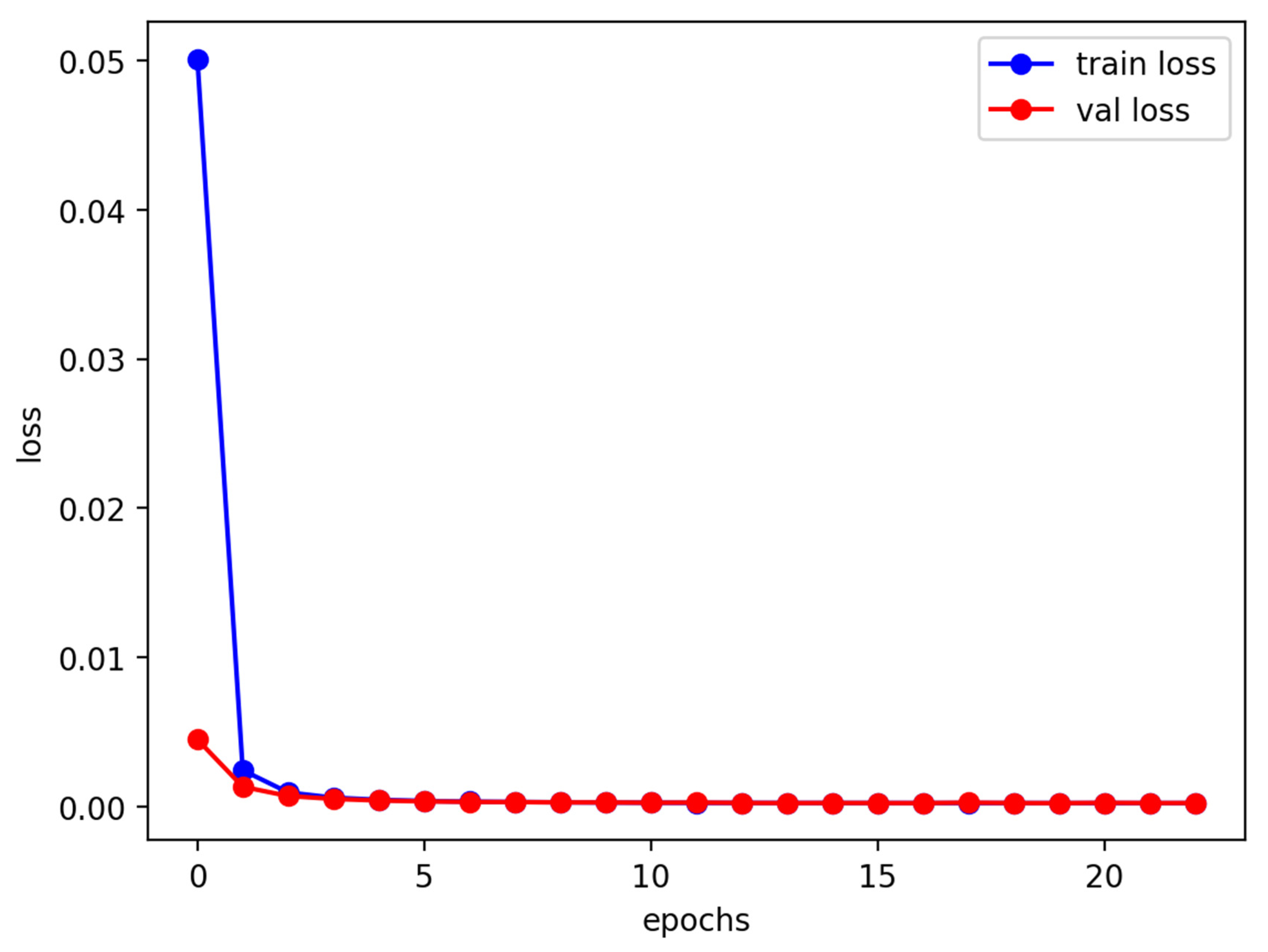
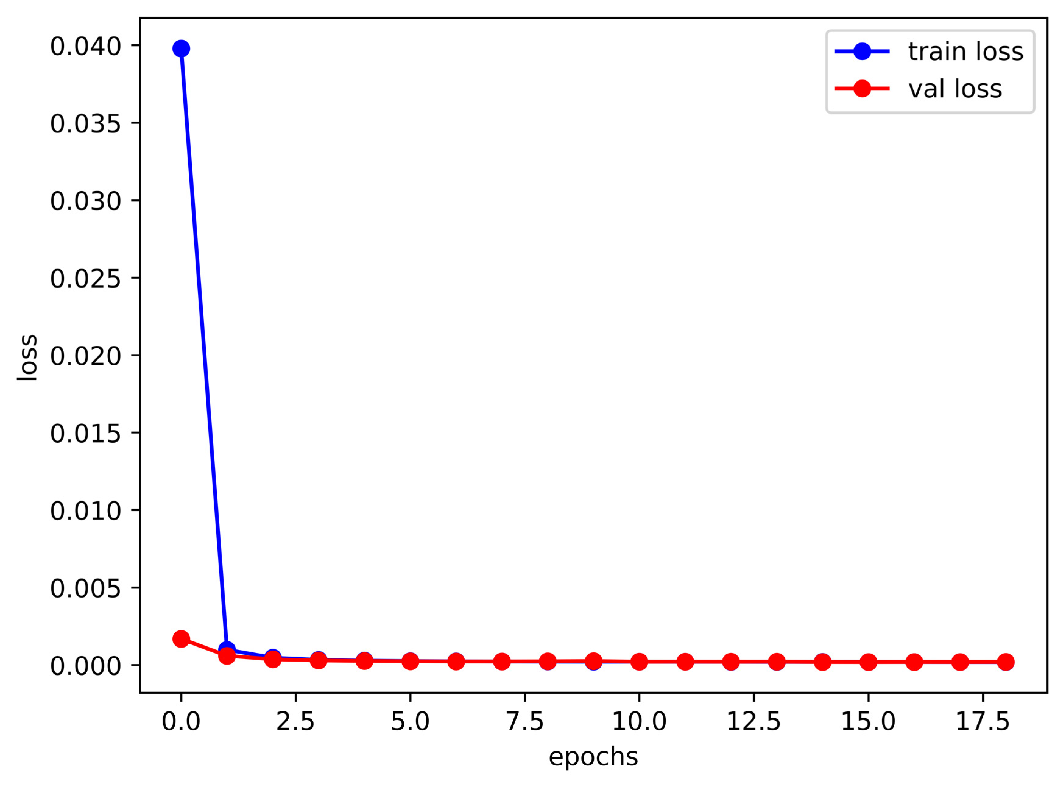
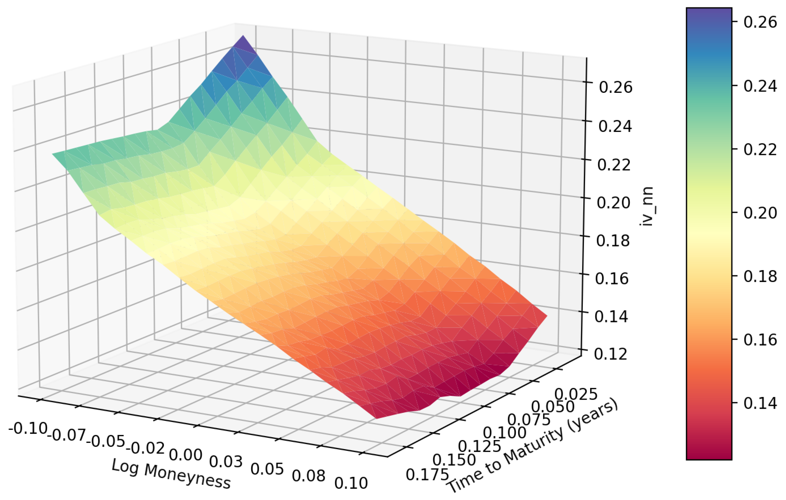
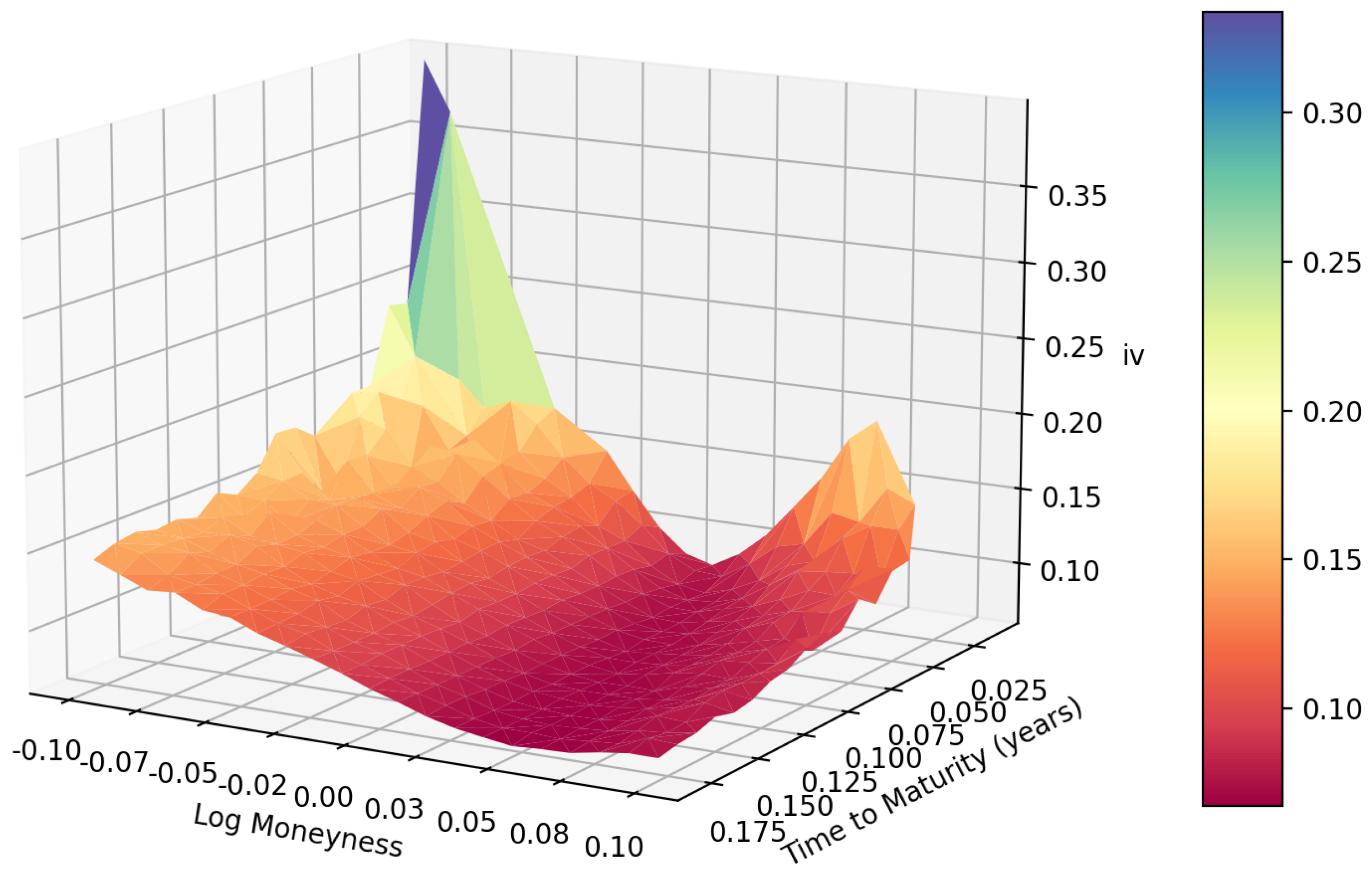
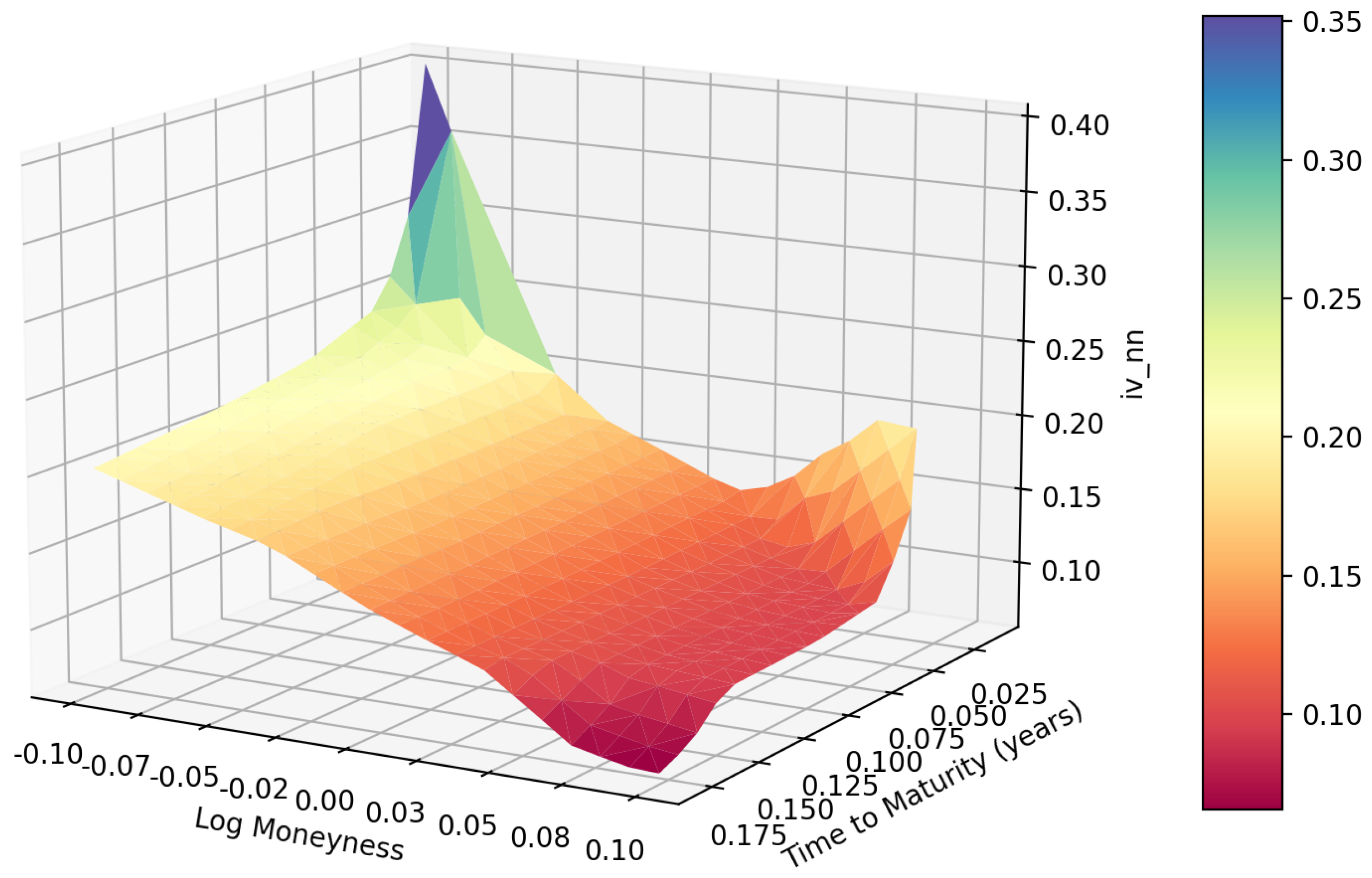
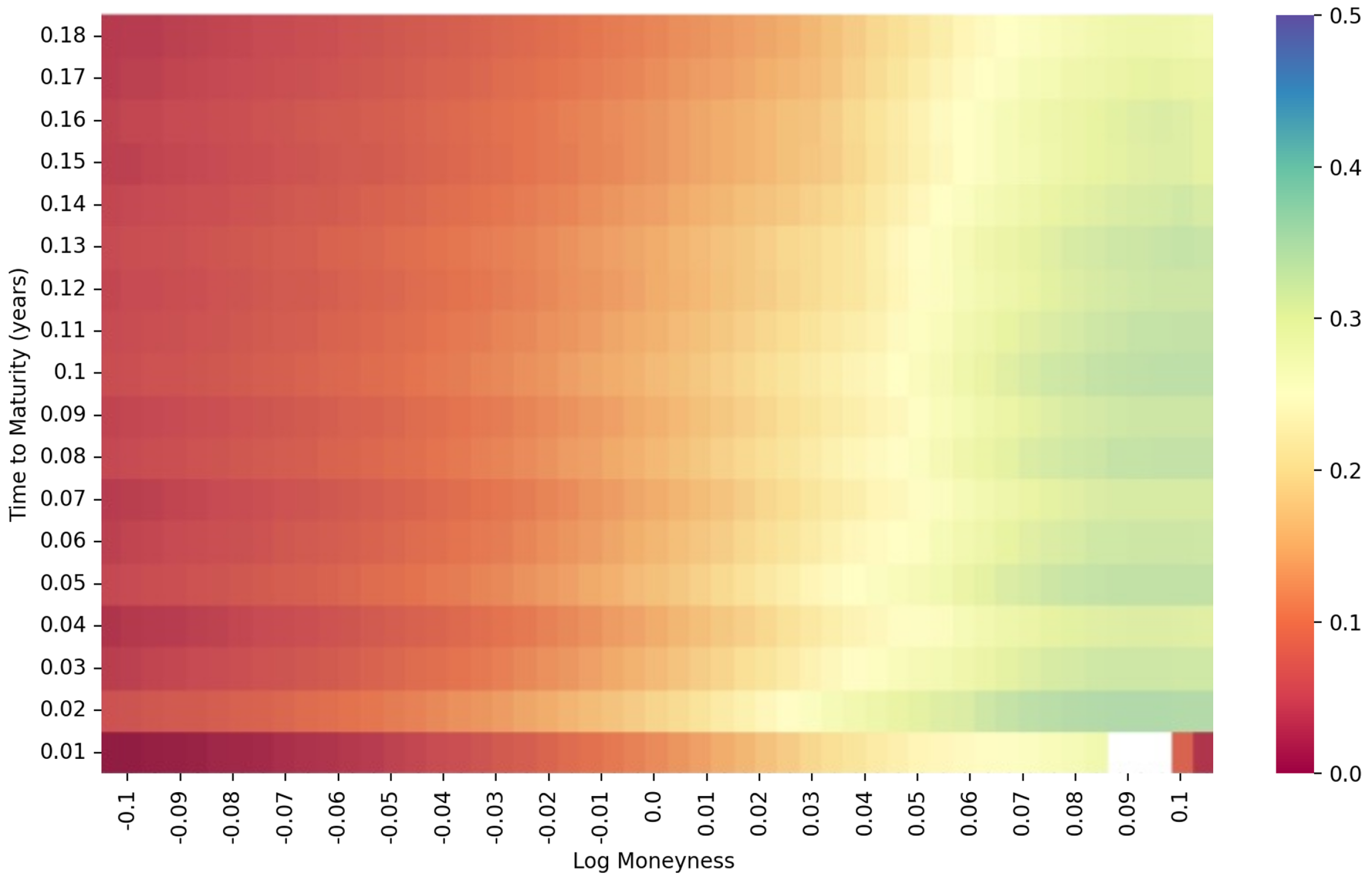
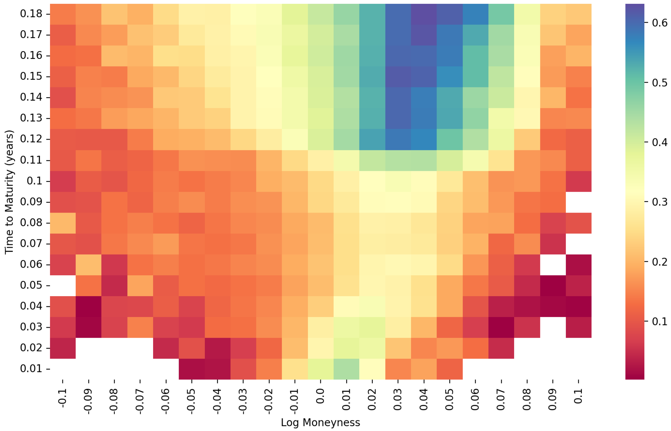
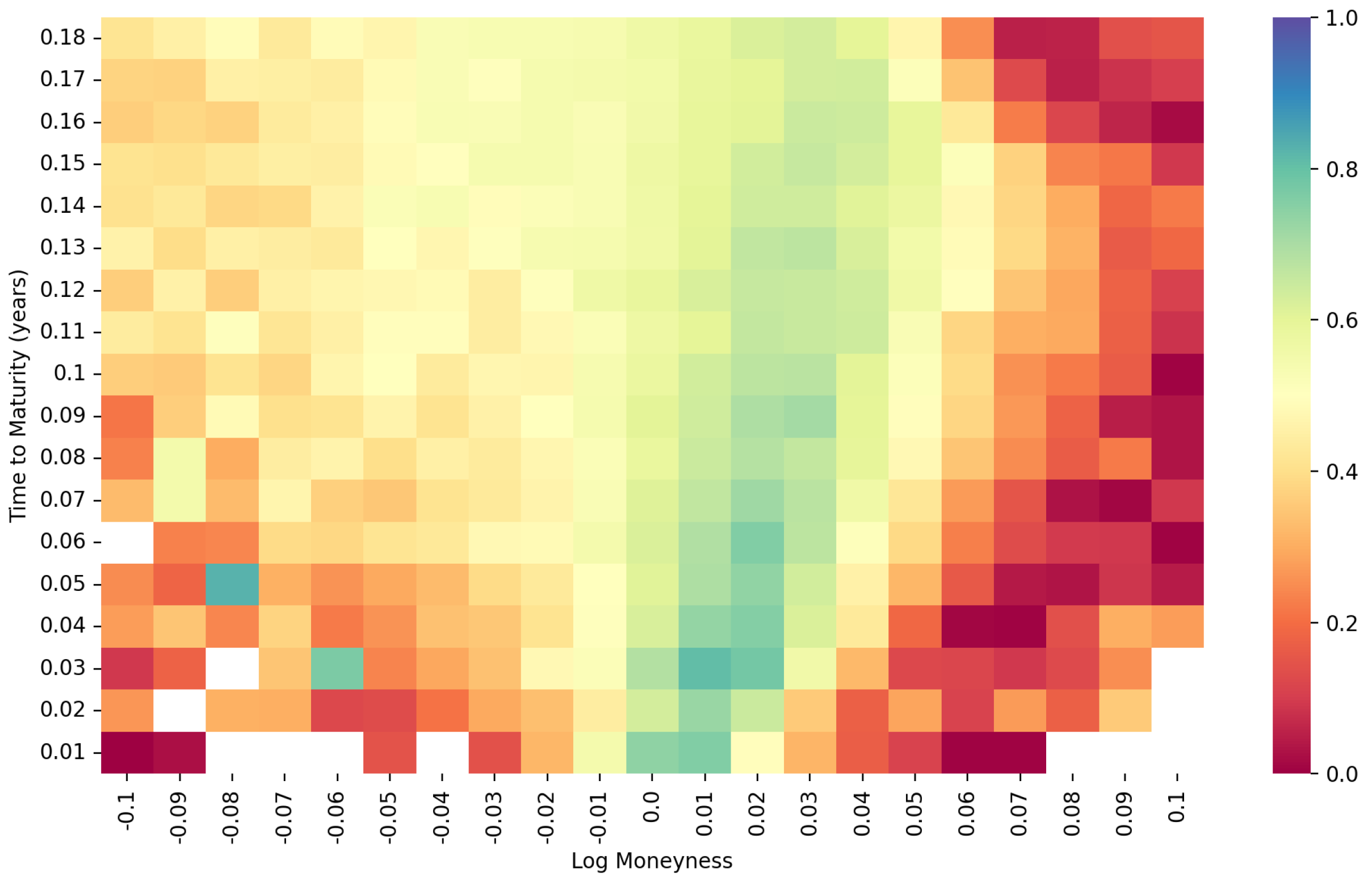
Here, we assess the performance of the deep calibration using the methods discussed in Section 3.1. We use the S&P options with maturities from 31 December 2021 to 15 December 2023, and FTSE options with maturities from 21 January 2022 to 15 December 2023, where the records with trading volume below two are removed. Figure 2 and Figure 3 show the FCNN’s deep calibration learning history under the rBergomi model. Figure 4, Figure 5, Figure 6 and Figure 7 give the IV surfaces generated by the parameters calibrated in Table 2 and Table 3. The details and parameters of the calibration process in this experiment are given below:
  • The heatmap of log moneyness and time to maturity under the Heston model, using S&P 500 data, is given in Figure 8.
  • The heatmaps of log moneyness and time to maturity under the rBergomi model, which are employed for the joint distribution’s estimation, are given in Figure 9 and Figure 10.
  • Set D is shuffled and partitioned into the training set, validation set and test set, as in Table 4.
  • The calibrated parameters ( H , η , ρ , V 0 ) are initialized as the truncated normal continuous random variables given in Table 5.
Following the deep calibration process introduced in Section 3.1, we can obtain the deep calibration performance of both the S&P data with maturities from 31 December 2021 to15 December 2023, and the FTSE data with maturities from 21 January 2022 to 15 December 2023. The first step is to generate the heatmap of time to maturity and log moneyness. As shown in Figure 8, the heatmap of the S&P data under the Heston model is very smooth except for the lower right corner. However, as shown in Figure 9 and Figure 10, the joint distributions under the rBergomi model form V-shaped patterns with the tips at the near-the-money short-dated locations, which are consistent with each other. We demonstrate the IV surfaces in Figure 4, Figure 5, Figure 6 and Figure 7, while parameters are given in Table 2 and Table 3.

4.2. Deep Hedging Performance under the rBergomi Model

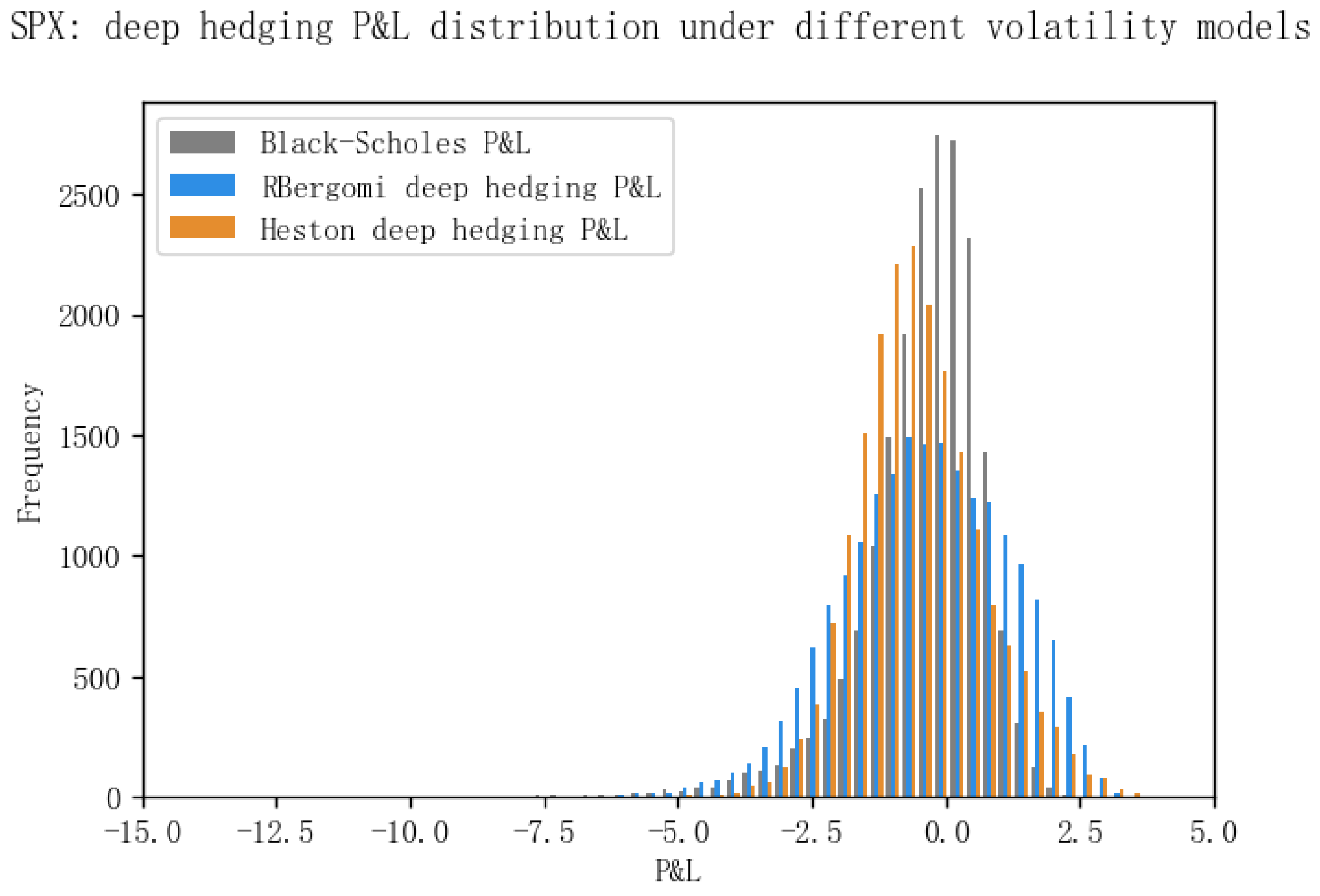
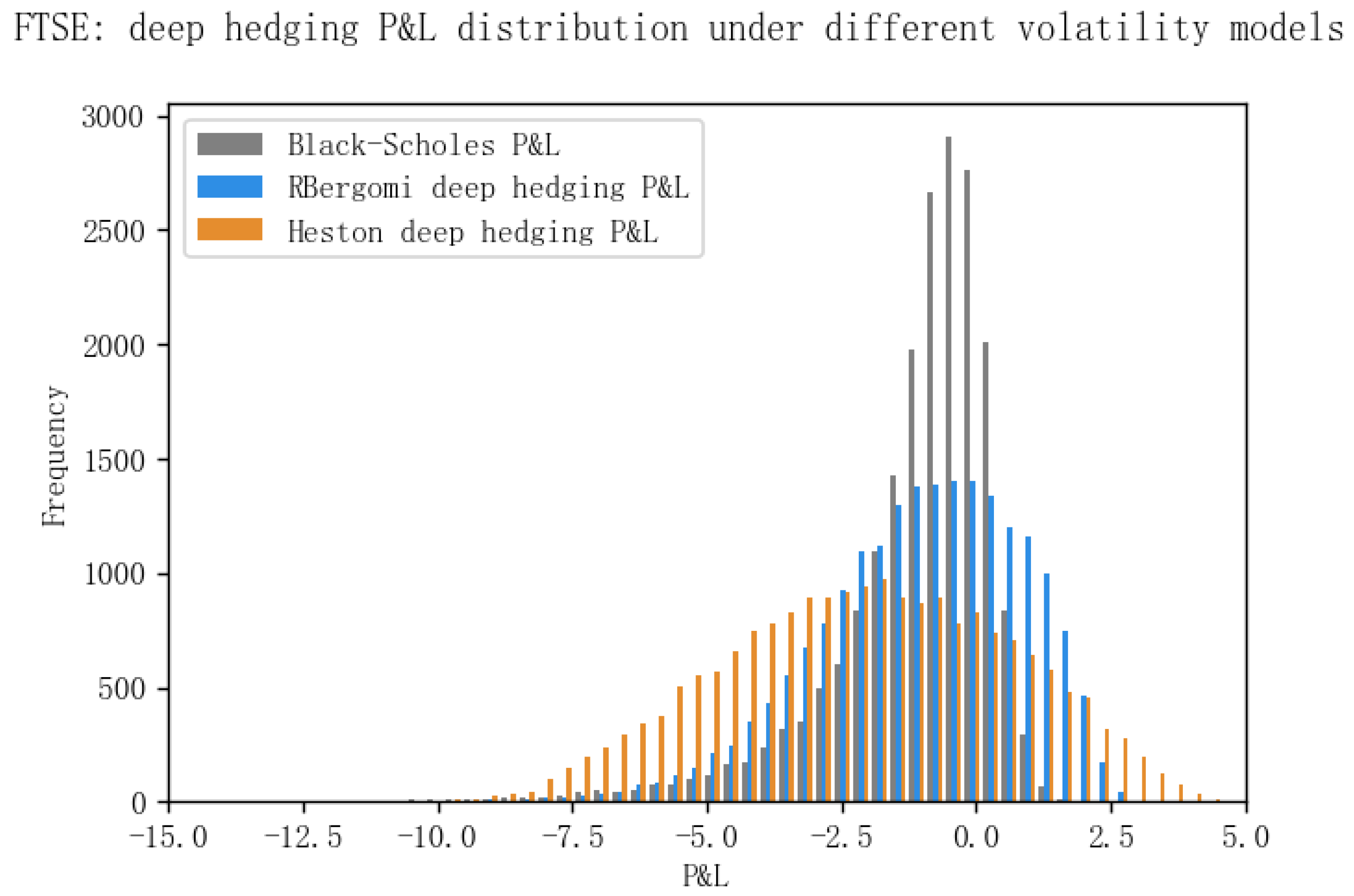
In the numerical experiment, we take the maturity T = 1 month and Dupire’s local volatility (see [36]) as the benchmark. We compare our results with the FRNN architecture proposed by [16] in Table 1. Thus, we set the neurons = 10 in the hidden state of our GRU-NN in the following experiment. The performance of the deep hedging using GRU-NN is illustrated by Figure 11 and Figure 12, which describe the profit and loss (P&L) distribution of the portfolio over the predetermined horizon.
Value-at-Risk (VaR) has become the industry’s benchmark as the tool of financial risk measurement. The traditional VaR models for estimating a portfolio’s P&L distribution can be divided approximately into the following three groups:
  • Parametric methods based on the assumption of conditional normality and economic models for volatility dynamics.
  • Methods based on simulations, e.g., Historical Simulation (HS) and Monte Carlo Simulation (MCS).
  • Methods based on Extreme Value Theory (EVT).
There are some parametric VaR models, such as GARCH models. Nevertheless, the primary shortcoming of those models is the conditional normality assumption. Such models may be better suited for estimating the distribution of large percentiles of the portfolio’s P&L distribution; see [37]. Unlike parametric VaR models, HS does not need a particular underlying asset returns distribution and is easier to perform; see [38]. Nonetheless, it has a few disadvantages. Most importantly, equivalent weights are utilized for returns during the whole period in the application, which contradicts the fact that the predictability of data is decreasing. As a result, most risk managers prefer a more quantitative approach.
It is observed that traditional parametric and nonparametric methods can work efficiently in the empirical distribution area. However, they fit the extreme tails of the distribution poorly, placing them at a disadvantage in extreme risk management. The last type of method, based on EVT, focuses on modelling the tail behavior of a loss distribution using only extreme values rather than the whole data set; see [39]. However, there remain two disadvantages of the EVT methods in practice. First, EVT methods are only appropriate if the original data set is reasonably large. In addition, EVT methods depend on the authenticity of the distribution that the raw data should follow.
However, in this paper, we estimate the P&L distribution under the rough volatility exemplified by the rBergomi model. This method is also a starting point for more applications in the field of risk management. Let Val t denote the portfolio’s value at t and Val t + 1 denote the value at t + 1 ; then, the P&L distribution is the distribution of ( Val t + 1 Val t ) . From Figure 11 and Figure 12, we notice that the P&L distribution of the GRU-NN deep hedging in the histogram is fat-tailed with a relatively heavier left tail. These features correspond to the financial markets’ phenomena exhibiting fatter tails than traditionally predicted. That is, for many financial assets, the probability of extreme returns occurring in reality is higher than the probability of extreme returns under the normal distribution. This feature is also referred to as leptokurtosis (see [40,41]).

5. Conclusions and Future Research

Which volatility model is the most suitable for hedging? Our paper is the first to provide a deep learning method (GRU-NN) for hedging and comparing volatility models with different regularities. We summarize the hedging performance and some other characteristics of different volatility models in Table 6 and Table 7, which reveal that the rBergomi model outperforms the other two models.
Due to these considerations, our paper can provide necessary value to practitioners and researchers.
Following the deep calibration procedure established in [15], we obtained the calibrated H , η , ρ , V 0 for the rBergomi model using the S&P option data with maturities from 31 December 2021 to 15 December 2023, and the FTSE option data with maturities from 21 January 2022 to 15 December 2023. After that, we developed a GRU-NN architecture to implement deep hedging. The apparent strength of this network is that the gated recurrent unit enables it to capture the non-Markovianity brought by the rBergomi model. There are multiple gate-variants of the GRU proposed to reduce computational expense, such as the GRU1, GRU2, and GRU3 in [42], and we reserve their application for future research.
VaR is a prominent measure of market risk and answers how much we can suffer from the loss of a given probability over a specific time horizon. It has become increasingly important since the Basel Committee stated that banks should be capable of covering losses on their trading portfolios over a ten-day horizon, 99 percent of the time. Nevertheless, methods based on assumptions of normal distributions are inclined to underestimate the tail risk. Traditional methods based on HS can only provide very imprecise estimates of tail risk. Methods based on EVT only work when the original data set is reasonably large and the raw data’s distribution is sufficiently authentic. We propose a quantitative method under the rough volatility implemented by deep learning techniques, which exhibits the financial market’s leptokurtosis feature. We give the analysis and algorithm of this method, but there is still room to study its accuracy and versatility in handling pricing and risk management.

Author Contributions

Conceptualization, Q.Z.; Formal analysis, Q.Z.; Writing—original draft, Q.Z.; Writing—review & editing, X.D.; Visualization, Q.Z.; Funding acquisition, X.D. All authors have read and agreed to the published version of the manuscript.

Funding

This research was funded by National Natural Science Foundation of China under grant number 71771147.

Data Availability Statement

The code and data used to generate the results for this paper are available here: https://github.com/wendy-qinwen/deep_hedging_rBergomi (accessed on 29 October 2022).

Conflicts of Interest

The authors declare no conflict of interest.

References

  1. Black, F.; Scholes, M. The Pricing of Options and Corporate Liabilities. J. Political Econ. 1973, 81, 637–654. [Google Scholar] [CrossRef] [Green Version]
  2. Hull, J.; White, A. The pricing of options on assets with stochastic volatilities. J. Financ. 1987, 42, 281–300. [Google Scholar] [CrossRef]
  3. Stein, E.M.; Stein, J.C. Stock price distributions with stochastic volatility: An analytic approach. Rev. Financ. Stud. 1991, 4, 727–752. [Google Scholar] [CrossRef]
  4. Bergomi, L. Smile Dynamics III. 2008. Available online: https://papers.ssrn.com/sol3/papers.cfm?abstract_id=1493308 (accessed on 29 October 2022).
  5. Bergomi, L. Smile Dynamics IV. 2009. Available online: https://papers.ssrn.com/sol3/papers.cfm?abstract_id=1520443 (accessed on 29 October 2022).
  6. Heston, S.L. A Closed-Form Solution for Options with Stochastic Volatility with Applications to Bond and Currency Options. Rev. Financ. Stud. 1993, 6, 327–343. [Google Scholar] [CrossRef] [Green Version]
  7. Guidolin, M.; Timmermann, A. Option prices under Bayesian learning: Implied volatility dynamics and predictive densities. J. Econ. Dyn. Control. 2003, 27, 717–769. [Google Scholar] [CrossRef] [Green Version]
  8. Gatheral, J.; Jaisson, T.; Rosenbaum, M. Volatility is rough. Quant. Financ. 2018, 18, 933–949. [Google Scholar] [CrossRef]
  9. El Euch, O.; Fukasawa, M.; Rosenbaum, M. The microstructural foundations of leverage effect and rough volatility. Financ. Stoch. 2018, 22, 241–280. [Google Scholar] [CrossRef] [Green Version]
  10. Rosenbaum, M.; Tomas, M. From microscopic price dynamics to multidimensional rough volatility models. Adv. Appl. Probab. 2021, 53, 425–462. [Google Scholar] [CrossRef]
  11. Dandapani, A.; Jusselin, P.; Rosenbaum, M. From quadratic Hawkes processes to super-Heston rough volatility models with Zumbach effect. Quant. Financ. 2021, 21, 1–13. [Google Scholar] [CrossRef]
  12. Bayer, C.; Friz, P.; Gatheral, J. Pricing under rough volatility. Quant. Financ. 2016, 16, 887–904. [Google Scholar] [CrossRef]
  13. Zhu, Q.; Loeper, G.; Chen, W.; Langrené, N. Markovian approximation of the rough Bergomi model for Monte Carlo option pricing. Mathematics 2021, 9, 528. [Google Scholar] [CrossRef]
  14. Hernandez, A. Model Calibration with Neural Networks. 2016. Available online: https://papers.ssrn.com/sol3/papers.cfm?abstract_id=2812140 (accessed on 29 October 2022).
  15. Bayer, C.; Horvath, B.; Muguruza, A.; Stemper, B.; Tomas, M. On deep calibration of (rough) stochastic volatility models. arXiv 2019, arXiv:1908.08806. [Google Scholar]
  16. Horvath, B.; Muguruza, A.; Tomas, M. Deep learning volatility: A deep neural network perspective on pricing and calibration in (rough) volatility models. Quant. Financ. 2021, 21, 11–27. [Google Scholar] [CrossRef]
  17. Stone, H. Calibrating rough volatility models: A convolutional neural network approach. Quant. Financ. 2020, 20, 379–392. [Google Scholar] [CrossRef] [Green Version]
  18. Lu, D.W. Agent inspired trading using recurrent reinforcement learning and lstm neural networks. arXiv 2017, arXiv:1707.07338. [Google Scholar]
  19. Jiang, Z.; Xu, D.; Liang, J. A deep reinforcement learning framework for the financial portfolio management problem. arXiv 2017, arXiv:1706.10059. [Google Scholar]
  20. Buehler, H.; Gonon, L.; Teichmann, J.; Wood, B. Deep hedging. Quant. Financ. 2019, 19, 1271–1291. [Google Scholar] [CrossRef]
  21. Horvath, B.; Teichmann, J.; Zuric, Z. Deep Hedging under Rough Volatility. Risk 2021, 9, 1–20. [Google Scholar]
  22. Chakrabarti, B.; Santra, A. Comparison of Black Scholes and Heston Models for Pricing Index Options. 2017. Available online: https://papers.ssrn.com/sol3/papers.cfm?abstract_id=2943608 (accessed on 29 October 2022).
  23. Jacquier, A.; Martini, C.; Muguruza, A. On VIX futures in the rough Bergomi model. Quant. Financ. 2018, 18, 45–61. [Google Scholar] [CrossRef] [Green Version]
  24. Bennedsen, M.; Lunde, A.; Pakkanen, M.S. Hybrid scheme for Brownian semistationary processes. Financ. Stoch. 2017, 21, 931–965. [Google Scholar] [CrossRef] [Green Version]
  25. Kurpiel, A.; Roncalli, T. Option Hedging with Stochastic Volatility. 1998. Available online: https://papers.ssrn.com/sol3/papers.cfm?abstract_id=1031927 (accessed on 29 October 2022).
  26. Hodges, S. Optimal replication of contingent claims under transaction costs. Rev. Future Mark. 1989, 8, 222–239. [Google Scholar]
  27. Davis, M.H.; Panas, V.G.; Zariphopoulou, T. European option pricing with transaction costs. SIAM J. Control Optim. 1993, 31, 470–493. [Google Scholar] [CrossRef] [Green Version]
  28. McCrickerd, R.; Pakkanen, M.S. Turbocharging Monte Carlo pricing for the rough Bergomi model. Quant. Financ. 2018, 18, 1877–1886. [Google Scholar] [CrossRef] [Green Version]
  29. He, K.; Zhang, X.; Ren, S.; Sun, J. Delving deep into rectifiers: Surpassing human-level performance on imagenet classification. In Proceedings of the IEEE International Conference on Computer Vision, Santiago, Chile, 7–13 December 2015; pp. 1026–1034. [Google Scholar]
  30. Hornik, K. Approximation capabilities of multilayer feedforward networks. Neural Netw. 1991, 4, 251–257. [Google Scholar] [CrossRef]
  31. Levenberg, K. A method for the solution of certain non-linear problems in least squares. Q. Appl. Math. 1944, 2, 164–168. [Google Scholar] [CrossRef] [Green Version]
  32. Marquardt, D.W. An algorithm for least-squares estimation of nonlinear parameters. J. Soc. Ind. Appl. Math. 1963, 11, 431–441. [Google Scholar] [CrossRef]
  33. Zaremba, W.; Sutskever, I.; Vinyals, O. Recurrent neural network regularization. arXiv 2014, arXiv:1409.2329. [Google Scholar]
  34. Boulanger-Lewandowski, N.; Bengio, Y.; Vincent, P. Modeling temporal dependencies in high-dimensional sequences: Application to polyphonic music generation and transcription. arXiv 2012, arXiv:1206.6392. [Google Scholar]
  35. Mikolov, T.; Joulin, A.; Chopra, S.; Mathieu, M.; Ranzato, M. Learning longer memory in recurrent neural networks. arXiv 2014, arXiv:1412.7753. [Google Scholar]
  36. Dupire, B. Pricing with a smile. Risk 1994, 7, 18–20. [Google Scholar]
  37. Danielsson, J.; De Vries, C.G. Value-at-risk and extreme returns. Ann. D’Econ. Stat. 2000, 20, 239–270. [Google Scholar] [CrossRef] [Green Version]
  38. Cui, Z.; Kirkby, J.L.; Nguyen, D. A data-driven framework for consistent financial valuation and risk measurement. Eur. J. Oper. Res. 2021, 289, 381–398. [Google Scholar] [CrossRef]
  39. Gilli, M. An application of extreme value theory for measuring financial risk. Comput. Econ. 2006, 27, 207–228. [Google Scholar] [CrossRef] [Green Version]
  40. Carol, A. Market Models: A Guide to Financial Data Analysis; John Willer & Sons: New York, NY, USA, 2001. [Google Scholar]
  41. Cui, X.; Sun, X.; Zhu, S.; Jiang, R.; Li, D. Portfolio optimization with nonparametric value at risk: A block coordinate descent method. Inf. J. Comput. 2018, 30, 454–471. [Google Scholar] [CrossRef]
  42. Dey, R.; Salem, F.M. Gate-variants of gated recurrent unit (GRU) neural networks. In Proceedings of the 2017 IEEE 60th International Midwest Symposium on Circuits and Systems (MWSCAS), Boston, MA, USA, 6–9 August 2017; IEEE: Piscataway, NJ, USA, 2017; pp. 1597–1600. [Google Scholar]
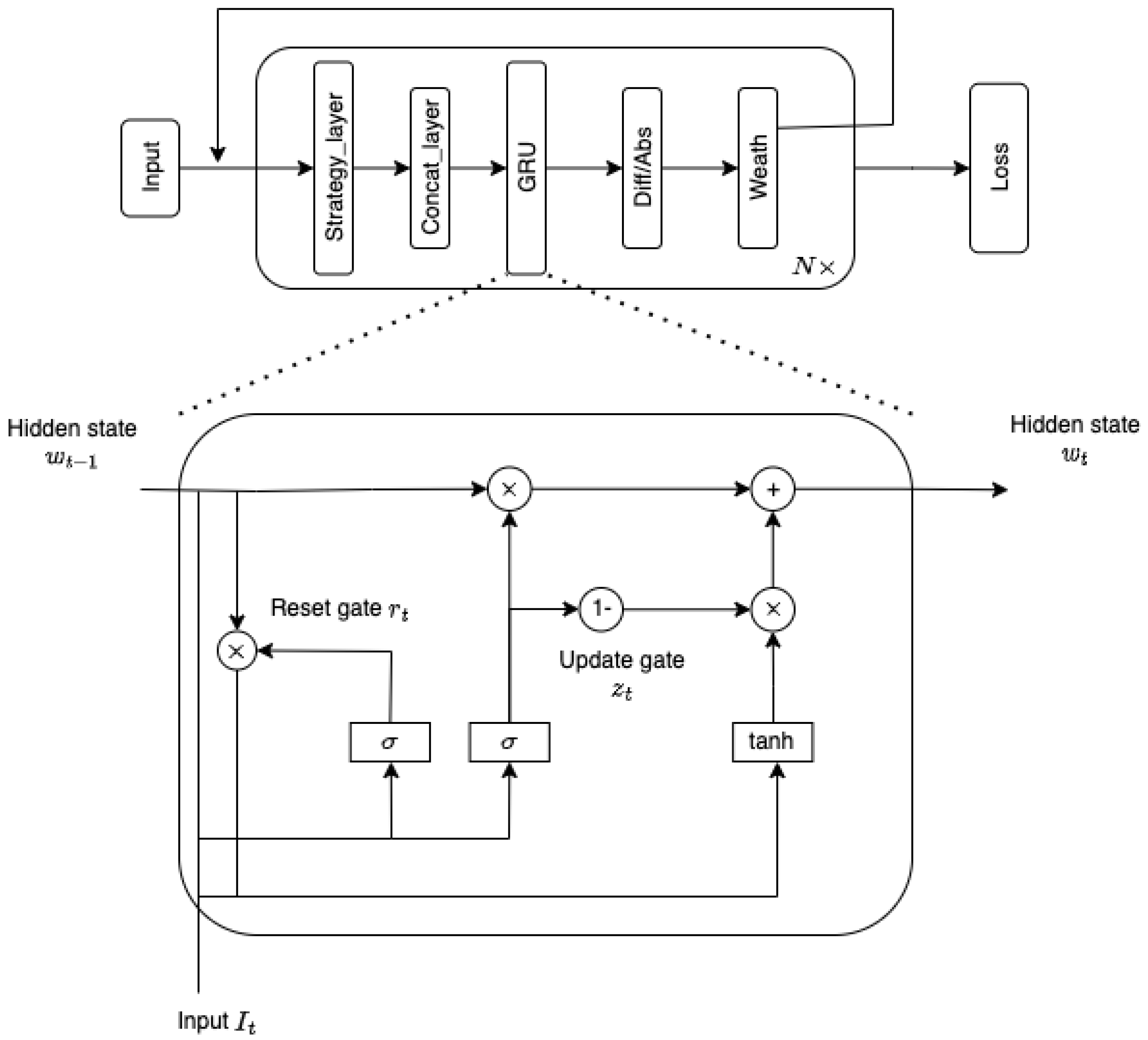
Figure 1. GRU–NN architecture for the deep hedging.
Fractalfract 07 00225 g001
Figure 2. Entropy losses for the S&P 500 data with maturities from 31 December 2021 to 15 December 2023.
Fractalfract 07 00225 g002
Figure 3. Entropy losses for the FTSE 100 data with maturities from 21 January 2022 to 15 December 2023.
Fractalfract 07 00225 g003
Figure 4. The Heston model’s IV surface inverted from S&P options data.
Fractalfract 07 00225 g004
Figure 5. The Heston model’s IV surface inverted from S&P options data by FCNN.
Fractalfract 07 00225 g005
Figure 6. The rBergomi model’s IV surface inverted from S&P options data.
Fractalfract 07 00225 g006
Figure 7. The rBergomi model’s IV surface inverted from S&P options data by FCNN.
Fractalfract 07 00225 g007
Figure 8. Heatmap of the S&P 500 data under the Heston model.
Fractalfract 07 00225 g008
Figure 9. Heatmap of the S&P 500 data under the rBergomi model.
Fractalfract 07 00225 g009
Figure 10. Heatmap of the FTSE 100 data under the rBergomi model.
Fractalfract 07 00225 g010
Figure 11. P&L distribution for the S&P options data with maturities from 31 December 2021 to 15 December 2023.
Fractalfract 07 00225 g011
Figure 12. P&L distribution for the FTSE options data with maturities from 21 January 2022 to 15 December 2023.
Fractalfract 07 00225 g012
Table 1. Comparison of the deep hedge entropy losses for different architecture types on 50 epochs.
ArchitectureTraining LossValidation LossTraining Time (s)
FRNN6.63906.46111548.17293
GRU-NN (5 neurons)6.34756.4465904.23617
GRU-NN (10 neurons)6.33426.4284913.25348
GRU-NN (15 neurons)6.58216.7498923.68151
GRU-NN (30 neurons)7.90717.2206962.75918
Table 2. Reference parameters and calibrated parameters for the Heston model.
ParamsReference ParamsS&P: Calibrated ParamsFTSE: Calibrated Params
ρ −0.5−0.7608−0.6125
σ v 1.00.94440.2222
θ 0.10.14960.1211
κ 0.60.73790.2038
V 0 0.020.02620.0134
Table 3. Reference parameters and calibrated parameters for the rBergomi model.
ParamsReference ParamsS&P: Calibrated ParamsFTSE: Calibrated Params
H0.070.0839620.088832
η 1.91.6314381.530887
ρ −0.9−0.929407−0.929521
V 0 0.2 2 0.112605 2 0.113197 2
Table 4. The partition of the set D .
SubsetsSizes
D train 450,000
D validation 25,000
D test 24,967
Table 5. Parameter initialization.
ParameterTruncated Normal Distribution
H N trunc [−1.2,8.6,0.07,0.05]
ρ N trunc [−0.25, 2.25, −0.95, 0.2]
η N trunc [−3, 3, 2.5, 0.5]
V 0 N trunc [−2.5, 7, 0.3, 0.1] 2
Table 6. Hedging performance summary.
ModelDataMeanStdVaR 0.99VaR 0.95VaR 0.90
Black–ScholesS&P 500−0.39341.17764.55062.46381.7089
FTSE 100−1.15111.71307.76976.43985.6278
HestonS&P 500−0.54101.14833.15122.35101.9326
FTSE 100−2.05252.70447.67764.28793.0168
rBergomiS&P 500−0.38471.56054.38892.96732.3806
FTSE 100−1.05641.93756.43654.46833.6126
Table 7. Summary of the characteristics of volatility models with different roughness scales.
CharacteristicsBlack–ScholesHestonrBergomi
Markovian
Semi-martingale
Regularity of the volatilityConstant H = 0.5 H 0.1
Skewness★★
Simulation speed★★
Microstructural explanation for the volatility★★
Accounts for variations in asset prices and price volatility★★
IV surface simulation★★
Fit short maturities★★
Number of parameters to be calibrated★★
Hedging performance (Delta, OCE)★★
Notes: ✩,★,★★ indicate the gradually better qualities. ✔ means “Yes” and ✘ means “No”.
Disclaimer/Publisher’s Note: The statements, opinions and data contained in all publications are solely those of the individual author(s) and contributor(s) and not of MDPI and/or the editor(s). MDPI and/or the editor(s) disclaim responsibility for any injury to people or property resulting from any ideas, methods, instructions or products referred to in the content.