

Generalized Beta Models and Population Growth: So Many Routes to Chaos

 ,
,  , , and
Abstract
1. Introduction
1.1. From Fibonacci Unbound Growth to Verhulst Sustainable Logistic Growth and Gompertz Extreme Growth
1.2. BetaBoop Functions
1.3. Review Organization
2. From Uniforms to BetaBoops—An Overview
- 1.
- , generalized logarithmic PDFs, the subfamily of power-logarithmic PDFs,
- 2.
- , the subfamily of PDFs;
- 3.
- , the PDFs;
- 4.
- , the positive power PDFs, the subfamily of PDFs;
- 5.
- , reverted generalized logarithmic PDFs, the subfamily of
2.1. BetaBoop , BetaBoop and Power Laws
3. BetaBoop(1,q,1,1), Fractional Calculus, Generalized Monotonicity and Convexity, and Applications in Probability Theory
3.1. Fractional Calculus and Some Applications in Probability Theory
- 1.
- ;
- 2.
- ;
- 3.
- .
3.2. Higher-Order Monotone Functions, Generalized Convexity, and Applications in Probability Theory
3.3. Fractional Powers of BetaBoop Random Variables
4. Logistic Growth, Gompertz Growth, and Extensions of the Logistic Map
5. Stable and Geo-stable EV Distributions
5.1. Extremes of IID Sequences
- min-Fréchet- distributions: ;
- min-Gumbel distribution: ;
- Weibull- distributions: .
5.2. Extremes of Geometrically Thinned Sequences
5.3. Verhulst Growth and Thinned Maxima, Gompertz Growth, and Maxima of IID Sequences
6. Population Growth Models and New Routes to Chaos
6.1. Generalized Logistic Population Models
- 1.
- , the model , investigated by Richards [30], with solution , where , i.e., the initial population size. The special case is the Verhulst logistic model, and the special case and is the Malthus exponential growth model.
- 2.
- 3.
- , the model , , extensively studied by Turner et al. [17,18] under the name generic growth function, with solutionThe case (i.e., ) is tied to the PDF of the Kumaraswamy RV.
- 4.
- If , the model (for , this is the Gompertz model). If , this hyper-Gompertz DE has the solutionFor , this is the Gompertz model.
6.2. The Logistic Paradigm and Extensions
6.2.1. Logistic Growth
6.2.2. Gompertz and Hyper-Logistic Growth
6.2.3. The Logistic Map with Random Reproducing Rate
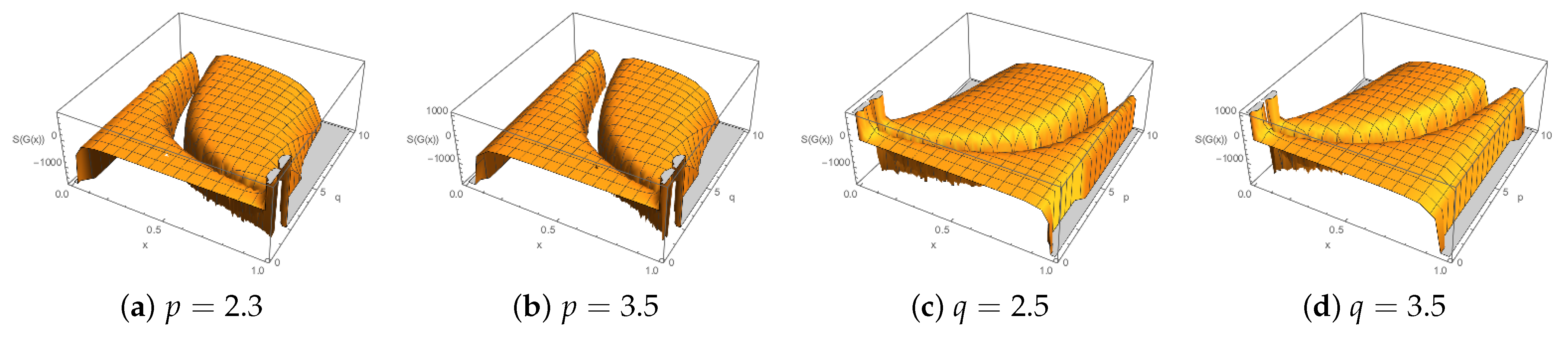
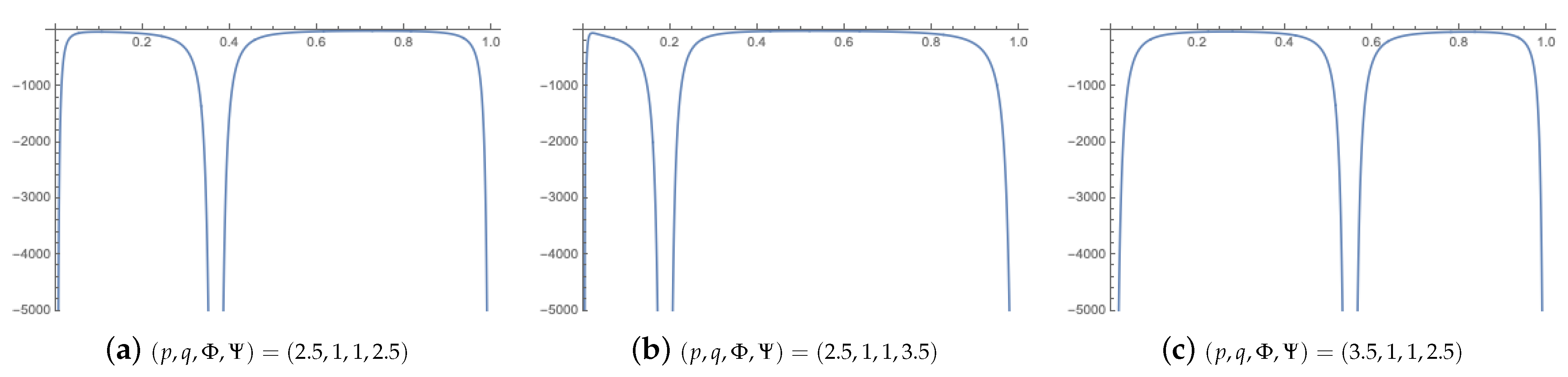
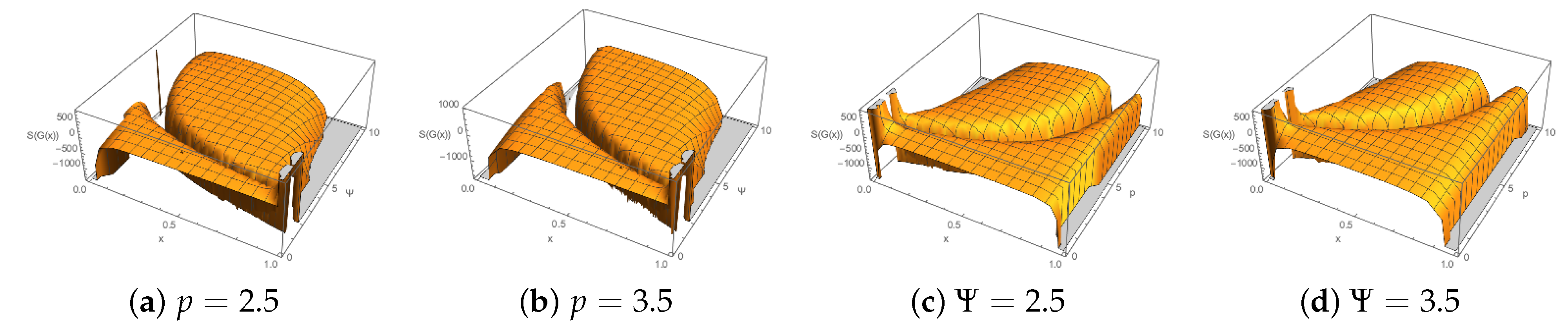
6.2.4. Schwarzian Derivative of Hyper-Logistic and Hyper-Gompertz Maps
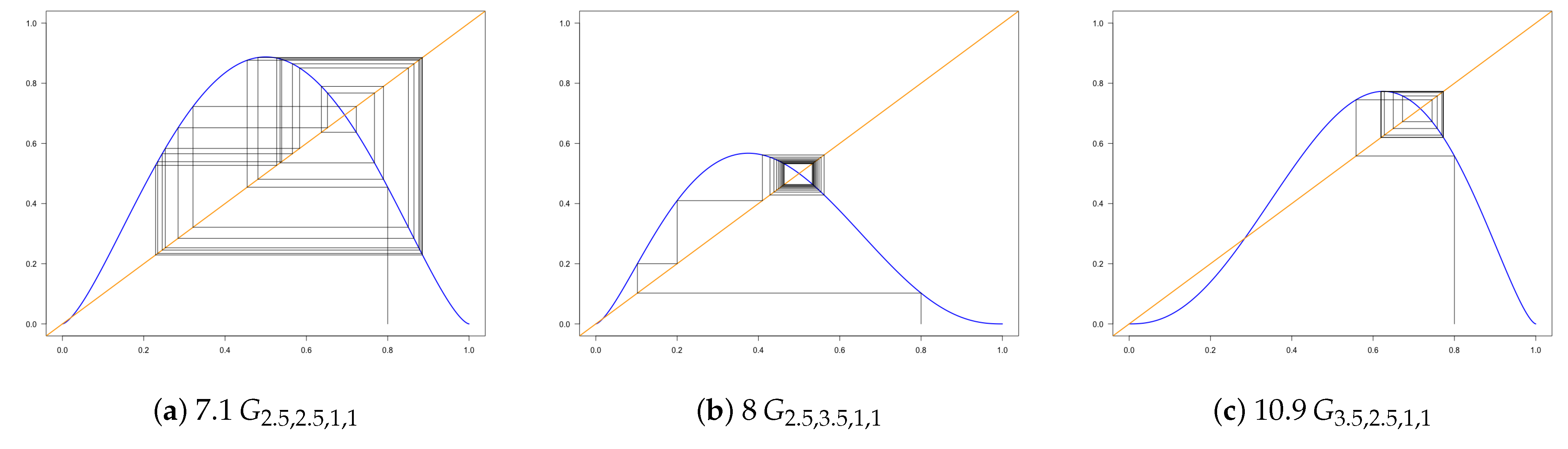
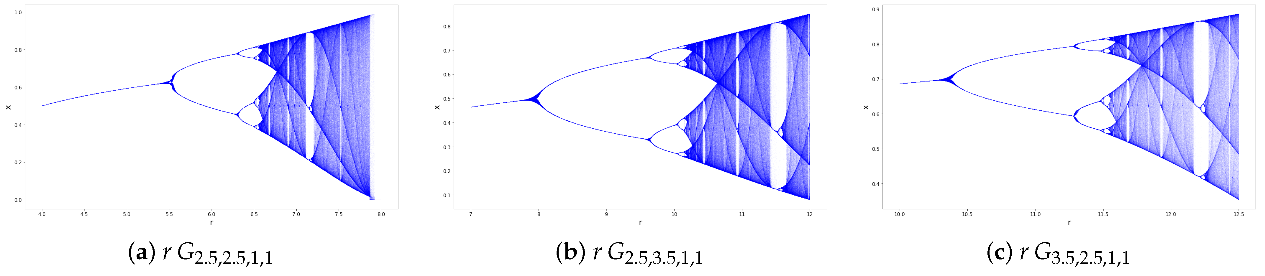
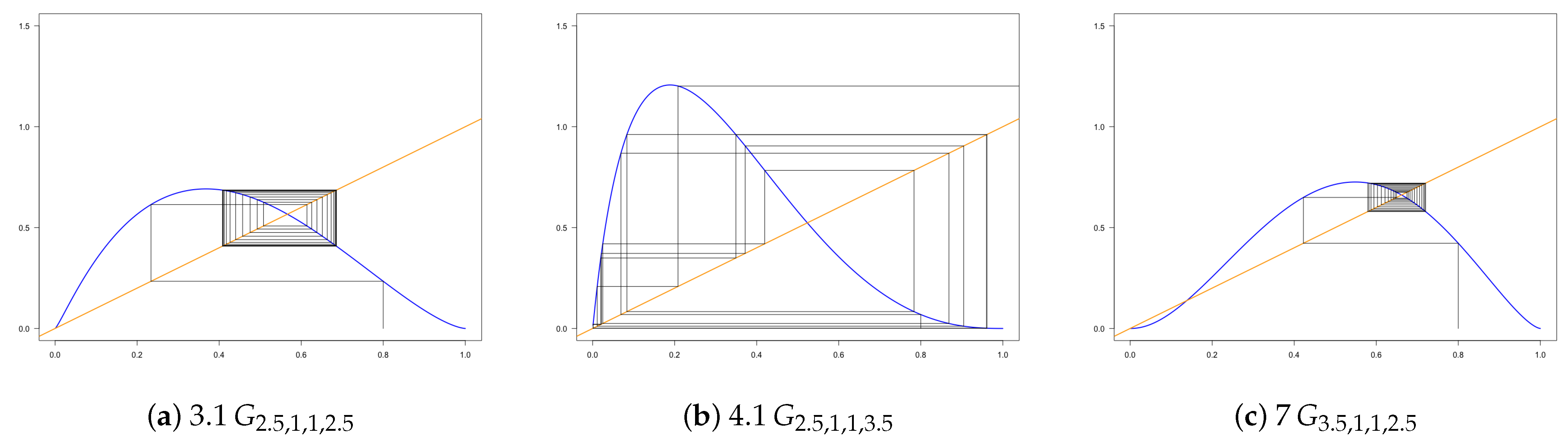
6.2.5. Hyper-Logistic Maps
6.2.6. Hyper−Gompertz Maps
6.3. Population Growth Models and EV Distributions
6.3.1. Blumberg Equation and Geo-Extreme Models
- When , we get a solution that is proportional to the log-logistic CDF with shape parameter , location parameter , and scale parameter ;
- When , we get a solution that is proportional to the backward log-logistic CDF with shape parameter , location parameter , and scale parameter ;
- When , the solution of the Verhulst equation is proportional to the logistic CDF.
6.3.2. Turner Equation and EV Models
- When , the solution is proportional to the min-Fréchet CDF with shape parameter , location parameter , and scale parameter ;
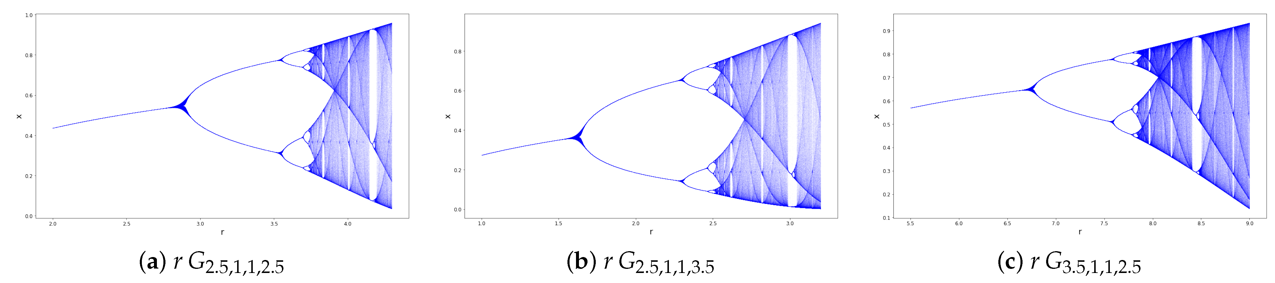
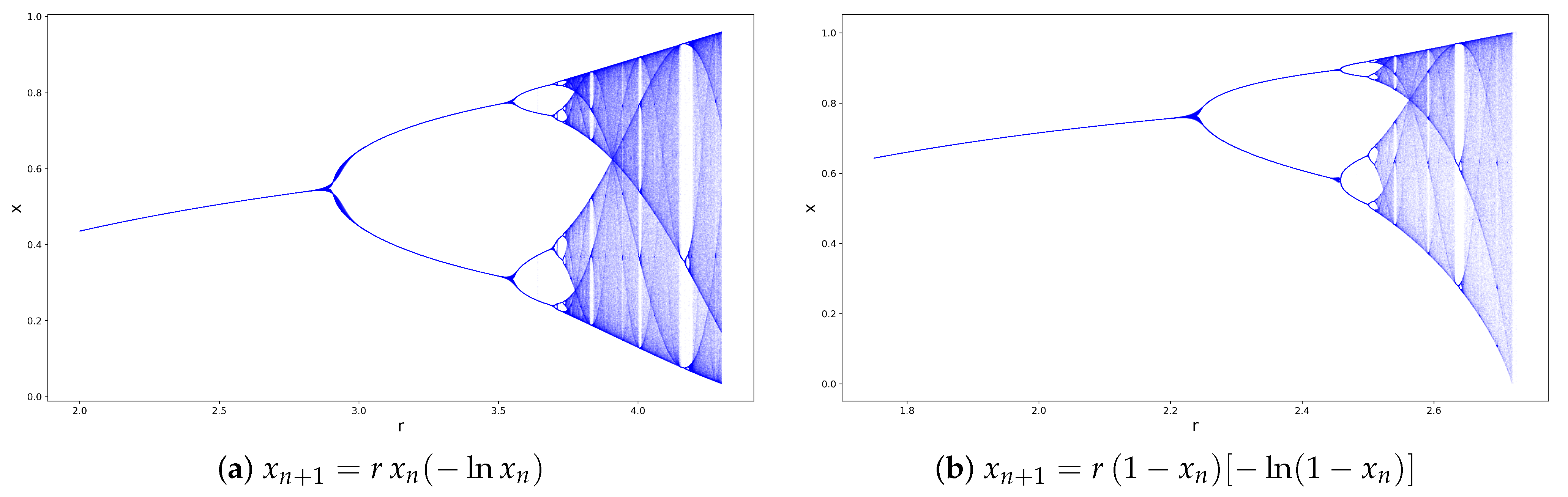
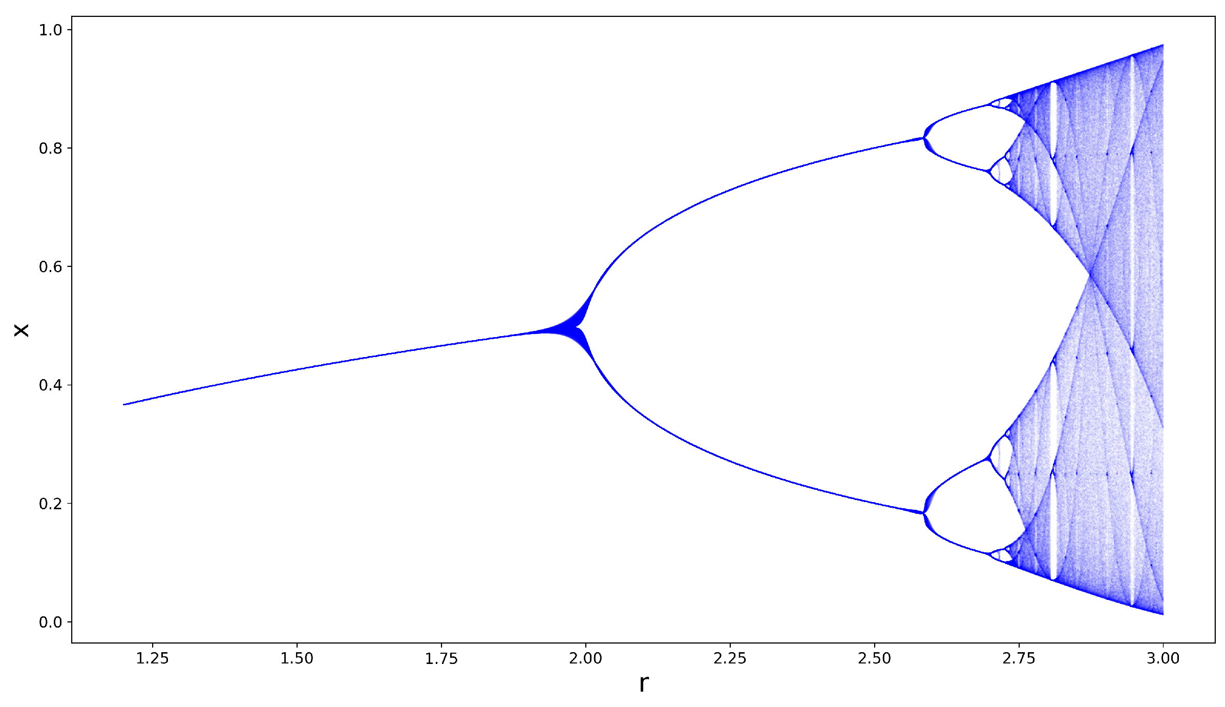
- When , the solution is proportional to the Weibull CDF with shape parameter , location parameter , and scale parameter .Figure 14 exhibits the pattern of bifurcations and ultimate chaos of the Turner map (see also the animation in Supplementary materials showing the corresponding evolution of different initial conditions as a function of r) and of the modified Turner map .
6.4. Chaos, Indeed?
7. Conclusions and Open Problems
Supplementary Materials
Author Contributions
Funding
Institutional Review Board Statement
Informed Consent Statement
Data Availability Statement
Acknowledgments
Conflicts of Interest
Abbreviations
| CDF | cumulative distribution function |
| DE | differential equation |
| EV | extreme value |
| EVT | extreme value theory |
| GEV | general extreme value |
| GMS | geo-max stable |
| IID | independent, identically distributed |
| MS | max-stable |
| OS | order statistic |
| probability density function | |
| RV | random variable |
Appendix A
- 1.
- If then conditions and are both verified, since .
- 2.
- If , then
- 3.
- If and , then and are verified if
- 4.
- If and , then and are verified if
- 1.
- However, from (A2),Hence, when , the integral (A7) is finite ifAgain, for from (A10), we get and, consequently,ifHence, when , the integral (A8) is finite if condition (A13) is satisfied.From (A12) and (A13),Finally,is finite, since is a continuous bounded function in We conclude that, when the integral (A6) is finite if
- 2.
- For or , we will use Hölder’s inequality a second time: let such that Then,If thenandand, consequently, we can conclude that, in this case,
- 3.
- If and then equality (A15) is verified ifHowever, and, from (A11),
- 4.
- The case and is similar to the previous case and we conclude that (A16) is verified if .
Appendix B. Blumberg Equation: Exponents Leading to Geo-Extreme Value Models
Appendix B.1. Blumberg Equation with p + q = 4
Appendix B.2. Verhulst Equation, p = q = 2
Appendix B.3. Pareto Populations
Appendix C. Turner’s Equation: Exponents Leading to Extreme Value Models
Appendix C.1. Gompertz Equation and Max-Gumbel Population
Appendix C.2. Turner Equation and Max-GEV Populations
Appendix C.3. Modified Gompertz Equation and Min-Gumbel Population
Appendix C.4. Modified Turner Equation and Min-GEV Populations
- When , the solution is proportional to the min-Fréchet CDF with shape parameter , location parameter , and scale parameter ;
- When , the solution is proportional to the Weibull CDF with shape parameter , location parameter , and scale parameter .
References
- de la Croix, D.; Michel, P. A Theory of Growth. Dynamics and Policy in Overlapping Generations; Cambridge University Press: Cambridge, UK, 2002. [Google Scholar]
- Michel, P.; Wigniolle, B. Une présentation simple des dynamiques complexes. Rev. Econ. 1993, 44, 885–911. [Google Scholar]
- Yang, R.C.; Kozak, A.; Smith, J.H.G. The potential of Weibull-type functions as flexible growth curves. Can. J. For. Res. 1978, 8, 424–431. [Google Scholar] [CrossRef]
- Payandeh, B.; Wang, Y. Comparison of the modified Weibull and Richards growth function for developing site index equations. New For. 1995, 9, 147–155. [Google Scholar] [CrossRef]
- Laird, A.K. Dynamics of tumour growth: Comparison of growth rates and extrapolation of growth curve to one cell. Br. J. Cancer 1965, 19, 278–291. [Google Scholar] [CrossRef]
- Laird, A.K.; Tyler, S.A.; Barton, A.D. Dynamics of normal growth. Br. J. Cancer 1965, 29, 233–248. [Google Scholar]
- Norton, L.; Simon, R.; Brereton, H.D.; Bogden, A.E. Predicting the course of Gompertzian growth. Nature 1976, 264, 542–545. [Google Scholar] [CrossRef]
- Bajzer, Z. Gompertzian growth as a self-similar and allometric process. Growth Dev. Aging 1999, 63, 3–11. [Google Scholar]
- Waliszewski, P.; Molski, M.; Konarski, J. On the holistic approach in cellular and cancer biology: Nonlinearity, complexity, and quasi-determinism of the dynamic cellular network. J. Surg. Oncol. 1998, 68, 70–78. [Google Scholar] [CrossRef]
- Waliszewski, P.; Molski, M.; Konarski, J. On the modification of fractal self-space during cell differentiation or tumor progression. Fractals 2000, 8, 195–203. [Google Scholar] [CrossRef]
- Waliszewski, P.; Konarski, J. Neuronal differentiation and synapse formation occur in space and time with fractal dimension. Synapse 2002, 43, 252–258. [Google Scholar] [CrossRef]
- Waliszewski, P.; Konarski, J. Gompertzian curve reveals fractal properties of tumor growth. Chaos Solitons Fractals 2003, 16, 665–674. [Google Scholar] [CrossRef]
- Waliszewski, P.; Konarski, J. A Mystery of the Gompertz Function. In Fractals in Biology and Medicine. Mathematics and Biosciences in Interaction; Losa, G.A., Merlini, D., Nonnenmacher, T.F., Weibel, E.R., Eds.; Birkhäuser: Boston, MA, USA, 2005; pp. 277–286. [Google Scholar]
- Molski, M.; Konarski, J. Tumor growth in the space-time temporal fractal dimension. Chaos Solitons Fractals 2008, 36, 811–818. [Google Scholar] [CrossRef]
- Tjørve, K.M.C.; Tjørve, E. The use of Gompertz models in growth analyses, and new Gompertz-model approach: An addition to the Unified-Richards family. PLoS ONE 2017, 12, e0178691. [Google Scholar] [CrossRef]
- Blumberg, A.A. Logistic growth functions. J. Theor. Biol. 1968, 21, 42–44. [Google Scholar] [CrossRef] [PubMed]
- Turner, M.E.; Blumenstein, B.A.; Sebaugh, J.L. A generalization of the logistic law of growth. Biometrics 1969, 25, 577–580. [Google Scholar] [CrossRef]
- Turner, M.E.; Bradley, E.L.; Kirk, K.A.; Pruitt, K.M. A theory of growth. Math. Biosci. 1976, 29, 367–373. [Google Scholar] [CrossRef]
- Brilhante, M.F.; Gomes, M.I.; Pestana, D. BetaBoop Brings in Chaos. CMSim—Chaotic Model. Simul. J. 2011, 1, 39–50. [Google Scholar]
- Brilhante, M.F.; Gomes, M.I.; Pestana, D. Extensions of Verhulst Model in Population Dynamics and Extremes. CMSim—Chaotic Model. Simul. J. 2012, 2, 575–591. [Google Scholar]
- Brilhante, M.F.; Gomes, M.I.; Pestana, D. Modelling risk of extreme events in generalized Verhulst models. Revstat Stat. J. 2019, 17, 145–162. [Google Scholar]
- Gomes, M.I.; Brilhante, M.F.; Pestana, D. Extensions of the Verhulst Model, Order Statistics and Products of Independent Uniform Random Variables. CMSim—Chaotic Model. Simul. J. 2014, 4, 315–322. [Google Scholar]
- von Foerster, H.; Mora, P.M.; Amiot, L.W. Doomsday: Friday, 13 November, A.D. 2026. Science 1960, 132, 1291–1295. [Google Scholar]
- Verhulst, P.-F. Notice sur la loi que la population poursuit dans son accroissement. Corresp. Math. Physics 1838, 113–121. [Google Scholar]
- Verhulst, P.-F. La loi de l’accroissement de la population. Nouv. Mem. Acad. R. Sci. Belles-Lett. Brux. 1845, 18, 1–42. [Google Scholar]
- Verhulst, P.-F. Deuxième mémoire sur la loi d’accroissement de la population. In Mémoires de l’Académie Royale des Sciences, des Lettres et des Beaux-Arts de Belgique; The European Digital Mathematics Library: Brussels, Belgium, 1847; Volume 20, pp. 1–32. [Google Scholar]
- May, R. Simple mathematical models with very complicated dynamics. Nature 1976, 261, 459–467. [Google Scholar] [CrossRef]
- Dubois, D.M. Recurrent generation of Verhulst chaos maps at any order and their stabilization diagram by anticipative control. In The Logistic Map and the Route to Chaos. Understanding Complex Systems; Ausloos, M., Dirickx, M., Eds.; Springer: Berlin/Heidelberg, Germany, 2006; pp. 53–75. [Google Scholar]
- Lorthois, S.; Cassot, F. Fractal analysis of vascular networks: Insights from morphogenesis. J. Theor. Biol. 2010, 262, 614–633. [Google Scholar] [CrossRef] [PubMed]
- Richards, F.J. A flexible growth functions for empirical use. J. Exp. Bot. 1959, 10, 290–300. [Google Scholar] [CrossRef]
- Whittaker, E.T.; Watson, G.N. A Course of Modern Analysis, 4th ed.; Cambridge University Press: Cambridge, UK, 1963. [Google Scholar]
- Erdélyi, A.; Magnus, W.; Oberhettinger, F.; Tricomi, F.G. Higher Transcendental Functions; McGraw-Hill: New York, NY, USA, 1953; Volume I. [Google Scholar]
- Borel, E. Les probabilités dénombrables et leurs applications arithmétiques. Rend. del Circ. Mat. di Palermo 1909, 27, 247–271. [Google Scholar] [CrossRef]
- Box, G.E.P.; Muller, M.E. A Note on the Generation of Random Normal Deviates. Ann. Math. Stat. 1958, 29, 610–611. [Google Scholar] [CrossRef]
- Johnson, N.L.; Kotz, S.; Balakrishnan, N. Continuous Univariate Distributions; Wiley: New York, NY, USA, 2018; Volume 2. [Google Scholar]
- Hadjisavvas, N.; Martinez-Legaz, J.E.; Penot, J.P. (Eds.) Generalized Convexity and Generalized Monotonicity; Springer: Berlin/Heidelberg, Germany, 2001; Volume 502. [Google Scholar]
- Kumaraswamy, P. A generalized probability density function for double-bounded random processes. J. Hydrol. 1980, 46, 79–88. [Google Scholar] [CrossRef]
- Rachev, S.T.; Resnick, S. Max-geometric infinite divisibility and stability. Commun. Stat. Stoch. Model. 1991, 7, 191–218. [Google Scholar] [CrossRef]
- Tsoularis, A.; Wallace, J. Analysis of logistic growth models. Math. Biosci. 2002, 179, 21–55. [Google Scholar] [CrossRef]
- Singer, D. Stable Orbits and Bifurcation of Maps of the Interval. SIAM J. Appl. Math. 1978, 35, 260–267. [Google Scholar] [CrossRef]
- Guckenheimer, J. Sensitive dependence on initial conditions for one-dimensional maps. Commun. Math. Phys. 1979, 70, 133–160. [Google Scholar] [CrossRef]
- Sharkovskii, A.N. Co-existence of cycles of a continuous mapping of the line into itself. Ukr. Math. J. 1964, 16, 61–71. [Google Scholar]
- Li, T.Y.; Yorke, J.A. Period three implies chaos. Am. Math. Mon. 1975, 82, 985–992. [Google Scholar] [CrossRef]
- Dubois, D.M. Review of incursive, hyperincursive and anticipatory system—Foundation of anticipation in electromagnetism. AIP Conf. Proc. 2000, 517, 3–30. [Google Scholar]
- Zolotarev, V.M. Mellin–Stieltjes Transforms in Probability Theory. Theory Probab. Appl. 1957, 2, 433–460. [Google Scholar] [CrossRef]
- Schroeder, M. Fractals, Chaos, Power Laws—Minutes from an Infinite Paradise; Dover Publications: Mineola, New York, USA, 2009. [Google Scholar]
- Karamata, J. Sur un mode de croissance régulière des fonctions. Mathematica 1930, 4, 38–53. [Google Scholar]
- Bingham, N.H.; Goldie, C.M.; Teugels, J.L. Regular Variation; Cambridge University Press: Cambridge, UK, 1987. [Google Scholar]
- Feller, W. On regular variation and local limit theorems. In Proceedings of the Fifth Berkeley Symposium on Mathematical Statistics and Probability, Berkeley, CA, USA, 21 June–18 July 1965; Neyman, J., Ed.; University of California Press: Berkeley, CA, USA, 1967; Volume II, pp. 373–388. [Google Scholar]
- Doeblin, W. Sur l’ensemble des puissances d’une loi de probabilités. Stud. Math. 1940, 9, 71–96. [Google Scholar] [CrossRef]
- Gnedenko, B.V. On the theory of domains of attraction of stable laws. Uchenye Zap. Moskov Gos. Univ. 1940, 30, 61–72. [Google Scholar]
- Gnedenko, B.V. Sur la distribution limite du terme maximum d’une série aléatoire. Ann. Math. 1943, 44, 423–453. [Google Scholar] [CrossRef]
- de Haan, L. On Regular Variation and Its Applications to the Weak Convergence of Sample Extremes; Mathematisch Centrum: Amsterdam, The Netherlands, 1970. [Google Scholar]
- Bingham, N.H. Factorisation theory and domains of attraction for generalised convolution algebras. Proc. Lond. Math. Soc. 1971, 23, 16–30. [Google Scholar] [CrossRef]
- Kozubowski, T.J.; Rachev, S.T. Univariate geometric stable distributions. J. Comput. Anal. Appl. 1999, 1, 177–217. [Google Scholar]
- Stanley, H.E. Scaling, universality and renormalization: Three pillars of modern critical phenomena. Rev. Mod. Phys. 1999, 71, 358–366. [Google Scholar] [CrossRef]
- Goursat, E. Cours d’Analyse Mathématique; Gabay: Paris, France, 1904. [Google Scholar]
- Ross, B. The development of fractional calculus 1695–1900. Hist. Math. 1977, 4, 75–89. [Google Scholar] [CrossRef]
- Liouville, J. Mémoire sur le calcul des différentielles à indices quelconques. Journal de l’École Polytechnique Paris 1832, 13, 71–162. [Google Scholar]
- Dugowson, S. Les Différentielles Métaphysiques (Histoire et Philosophie de la Généralisation de l’Ordre de Dérivation). Ph.D. Thesis, Université de Paris Nord, Paris, France, 1994. [Google Scholar]
- Area, I.; Nieto, J.J. Fractional-order logistic differential equation with Mittag-Leffler-type kernel. Fractal Fract. 2021, 5, 273. [Google Scholar] [CrossRef]
- Lavoie, J.L.; Osler, T.J.; Tremblay, R. Fractional derivatives and special functions. SIAM Rev. 1976, 18, 240–268. [Google Scholar] [CrossRef]
- Luchko, Y. Fractional Integrals and Derivatives: “True" versus “False"; MDPI: Basel, Switzerland, 2021. [Google Scholar]
- Pestana, D. Some Contributions to Unimodality, Infinite Divisibility and Related Topics. Ph.D. Thesis, University of Sheffield, Sheffield, UK, 1978. [Google Scholar]
- Gomes, M.I.; Pestana, D. The use of fractional calculus in Probability Theory. Port. Math. 1978, 37, 259–271. [Google Scholar]
- Lévy, P. Sur une application de la dérivée d’ordre non entier au calcul des probabilités. C. R. Acad. Sci. Paris 1923, 176, 1118–1120. [Google Scholar]
- Feller, W. On a generalization of Marcel Riesz’ potentials and the semi-groups generated by them. In Meddelanden Lunds Universitetes Matematiska Seminarium; Supplement Band Dedicated to M. Riesz, Gauthier-Villars; Lunds University: Paris, France, 1952; pp. 75–81. [Google Scholar]
- Wintner, A. On Heaviside’s and Mittag-Leffler’s generalization of the exponential function, the symmetric stable distributions of Cauchy-Lévy, and a property of the Γ-function. J. Math. Pures Appl. (Liouville) 1959, 38, 165–182. [Google Scholar]
- Wolfe, S.J. On Moments of Probability Distribution Functions; Lectures Notes in Mathematics; Springer: Berlin, Germany, 1975; Volume 457. [Google Scholar]
- Oldham, K.B.; Spanier, J. The Fractional Calculus; Theory and Applications of Differentiation and Integration to Arbitrary Order; Dover Publications: Mineola, NY, USA, 2006. [Google Scholar]
- Samko, S.G.; Kilbas, A.A.; Marichev, O.I. Fractional Integrals and Derivatives: Theory and Applications; Gordon and Breach: New York, NY, USA, 1993. [Google Scholar]
- Daftardar-Gejji, V. Fractional Calculus: Theory and Applications; Narosa Publishing House: New Delhi, India, 2013. [Google Scholar]
- Katugampola, U.N. A New Approach To Generalized Fractional Derivatives. Bull. Math. Anal. Appl. 2014, 6, 1–15. [Google Scholar]
- Herrmann, R. Fractional Calculus—An Introduction for Physicists; World Scientific: Toh Tuck Link, Singapore, 2018. [Google Scholar]
- Bernstein, S.N. Sur les fonctions absolument monotones. Acta Math. 1928, 52, 1–66. [Google Scholar] [CrossRef]
- Feller, W. An Introduction to Probability Theory and Its Applications; Wiley: New York, NY, USA, 1971; Volume II. [Google Scholar]
- Pestana, D.; Mendonça, S. Higher-order monotone functions and Probability Theory. In Generalized Convexity and Generalized Monotonicity; Hadjisavvas, N., Martinez-Legaz, J.E., Penot, J.-P., Eds.; Springer: Berlin/Heidelberg, Germany, 2001; Volume 502, pp. 317–331. [Google Scholar]
- Choquet, G. Lectures on Analysis, II; Benjamin: New York, NY, USA, 1969. [Google Scholar]
- Phelps, R.R. Lectures on Choquet’s Theorem; Springer: Berlin, Heidelberg, Germany, 2001. [Google Scholar]
- Khinchine, A.Y. On unimodal distributions. Trams. Res. Inst. Math. Mech. 1938, 2, 1–7. (In Russian) [Google Scholar]
- Pestana, D. A new proof of Khinchine’s theorem and concepts of unimodality. Port. Math. 1980, 39, 357–370. [Google Scholar]
- Olshen, R.A.; Savage, L.J. A generalized unimodality. J. Appl. Probab. 1970, 7, 21–34. [Google Scholar] [CrossRef]
- Pestana, D. A note on Pólya’s theorem. Trab. de Estad. y de Investig. Oper. 1984, 35, 104–111. [Google Scholar] [CrossRef]
- Sakovič, D.N. On the Characteristic Functions of Concave Distributions. Theor. Prob. Math. Statist. 1975, 6, 103–108. [Google Scholar]
- Roberts, A.W.; Varberg, D.E. Convex Funtions; Academic Press: New York, NY, USA, 1973. [Google Scholar]
- Vivas Cortez, M.J.; Hernández, J.E. Generalized Convexity: A Contemporary Vision about Convexity. 2017. Available online: https://www.researchgate.net/publication/325625874_Generalized_Convexity_A_contemporary_vision_about_Convexity (accessed on 9 November 2022).
- Sitthiwirattham, T.; Nonlaopon, K.; Ali, M.A.; Budak, H. Riemann-Liouville fractional Newton’s type Iinequalities for differentiable convex functions. Fractal Fract. 2022, 6, 175. [Google Scholar] [CrossRef]
- Sahoo, S.K.; Tariq, M.; Ahmad, H.; Kodamasingh, B.; Shaikh, A.A.; Botmart, T.; El-Shorbagy, M.A. Some novel fractional integral inequalities over a new class of generalized convex function. Fractal Fract. 2022, 6, 42. [Google Scholar] [CrossRef]
- Jones, M.C. Kumaraswamy’s distribution: A beta-type distribution with some tractability advantages. Stat. Methodol. 2009, 6, 70–81. [Google Scholar] [CrossRef]
- Tjørve, E.; Tjørve, K.M.C. A unified approach to the Richards-model family for use in growth analyses: Why we need only two model forms. J. Theor. Biol. 2010, 267, 417–425. [Google Scholar] [CrossRef]
- Peitgen, H.-O.; Jürgens, H.; Saupe, D. Chaos and Fractals, New Frontiers of Science; Springer: New York, NY, USA, 1992. [Google Scholar]
- Aleixo, S.M.; Rocha, J.L.; Pestana, D. Populational growth models proportional to beta densities with Allee effect. Am. Inst. Phys. 2008, 1124, 3–12. [Google Scholar]
- Aleixo, S.M.; Rocha, J.L.; Pestana, D. Dynamical behaviour in the parameter space: New populational growth models proportional to beta densities. In Proceedings of the ITI 2009, 31th International Conference on Information Technology Interfaces, Cavtat, Croatia, 22–25 June 2009; Luzar-Stiffler, V., Jarec, I., Bekic, Z., Eds.; IEEE: Piscataway, NJ, USA, 2009; pp. 213–218. [Google Scholar]
- Aleixo, S.M.; Rocha, J.L.; Pestana, D. Probabilistic Methods in Dynamical Analysis: Population Growths Associated to Models Beta (p,q) with Allee Effect. In Dynamics, Games and Science, in Honour of Maurício Peixoto and David Rand; Peixoto, M.M., Pinto, A.A., Rand, D.A.J., Eds.; Springer: New York, NY, USA, 2011; Chapter 5; Volume II, pp. 79–95. [Google Scholar]
- Rocha, J.L.; Aleixo, S.M. Dynamical analysis in growth models: Blumberg’s equation. Discret. Contin. Dyn. Syst. 2013, 18, 783–795. [Google Scholar]
- Pestana, D.; Aleixo, S.M.; Rocha, J.L. Regular variation, Paretian distributions, and the interplay of light and heavy tails in the fractality of asymptotic models. In Chaos Theory: Modeling, Simulation and Applications; Skiadas, C.H., Dimotikalis, I., Skiadas, C., Eds.; World Scientific Books: Singapore, 2011; pp. 309–316. [Google Scholar]
- Rocha, J.L.; Aleixo, S.M. An extension of Gompertzian growth dynamics: Weibull and Fréchet models. Math. Biosci. Eng. 2013, 10, 379–398. [Google Scholar]
- Fréchet, M. Sur la loi de probabilité de l’écart maximum. Ann. Soc. PoloNaise Math. 1927, 6, 93–116. [Google Scholar]
- Fisher, R.A.; Tippett, L.H.C. Limiting form of the frequency distribution of the largest or smallest member of a sample. Proc. Camb. Philos. Soc. 1928, 24, 180–190. [Google Scholar] [CrossRef]
- Davison, A.; Huser, R. Statistics of extremes. Annu. Rev. Stat. Its Appl. 2015, 2, 203–235. [Google Scholar] [CrossRef]
- Gomes, M.I.; Guillou, A. Extreme Value Theory and Statistics of Univariate Extremes: A Review. Int. Stat. Rev. 2015, 83, 263–292. [Google Scholar] [CrossRef]
- Rényi, A. A characterization of the Poisson process. MTA Mat. Kut. Int. Kozl. 1956, 1, 519–527. [Google Scholar]
- Kovalenko, I.N. On a class of limit distributions for rarefied flows of homogeneous events. Lit. Mat. Sb. 1965, 5, 569–573. [Google Scholar]
- Kozubowski, T.J. Representation and properties of geometric stable laws. In Approximation, Probability, and Related Fields; Anastassiou, G., Rachev, S.T., Eds.; Plenum: New York, NY, USA, 1994; pp. 321–337. [Google Scholar]
- Gnedenko, B.V.; Korolev, V.Y. Random Summation: Limit Theorems and Applications; CRC Press: Boca Raton, FL, USA, 1996. [Google Scholar]
- Resnick, S.I. Tail equivalence and its applications. J. Appl. Prob. 1971, 8, 136–156. [Google Scholar] [CrossRef]
- Resnick, S.I. Products of distribution functions attracted to extreme value laws. J. Appl. Prob. 1972, 8, 781–793. [Google Scholar] [CrossRef]
- Cline, D. Convolution tails, product tails and domains of attraction. Probab. Theor. 1986, 72, 529–557. [Google Scholar] [CrossRef]
- Bajzer, Z.; Vuk-Pavlovic, S.; Huzak, M. Mathematical modeling of tumor growth kinetics. In A Survey of Models for Tumor-Immune System Dynamics; Adam, J.A., Bellomo, N., Eds.; Birkhäuser: Boston, MA, USA, 1997; pp. 89–132. [Google Scholar]
- Mejzler, D. Extreme value limit laws in the nonidentically distributed case. Isr. J. Math. 1987, 57, 1–27. [Google Scholar] [CrossRef]
- Mejzler, D. Limit distributions for the extreme order statistics. Can. Math. Bull. 1978, 21, 447–459. [Google Scholar] [CrossRef]
- Mejzler, D. Asymptotic behaviour of the extreme order statistics in the non identically distributed case. In Statistical Extremes and Applications; Epstein, B., Tiago de Oliveira, J., Eds.; D. Reidel: Dordrecht, The Ntherlands, 1984; pp. 535–547. [Google Scholar]
- Graça Martins, M.E.; Pestana, D. Nonstable limit laws in Extreme Value Theory. In New Perspectives in Theoretical and Applied Statistics; Puri, M.L., Vilaplana, J.P., Wertz, W., Eds.; Wiley: Hoboken, NJ, USA, 1987; pp. 449–458. [Google Scholar]
- Urbanik, K. Limit laws for sequences of normed sums satisfying some stability conditions. In Multivariate Analysis III; Academic Press: Cambridge, MA, USA, 1973; pp. 225–237. [Google Scholar]
- Stephens, P.A.; Sutherland, W.J.; Freckleton, R.P. What is the Allee effect? Oikos 1999, 87, 185–190. [Google Scholar] [CrossRef]
- Berec, L.; Angulo, E.; Courchamp, F. Multiple Allee effects and population management. Trends Ecol. Evol. 2007, 22, 185–191. [Google Scholar] [CrossRef]
- Kramer, A.M.; Dennis, B.; Liebhold, A.M.; Drake, J.M. The evidence for Allee effects. Popul. Ecol. 2009, 51, 341–354. [Google Scholar] [CrossRef]
- Harrison, J. Wandering intervals. In Dynamical Systems and Turbulence; Warwick 1980. Lecture Notes in Mathematics; Rand, D., Young, L.S., Eds.; Springer: Berlin/Heidelberg, Germany, 1981; Volume 898. [Google Scholar]
- Cooper, B. The Schwarzian Derivative in One-Dimensional Dynamics. The University of Chicago Mathematics REU 2020: Participant Papers—Apprentice Program. 2020. Available online: https://math.uchicago.edu/~may/REU2020/REUPapers/Cooper.pdf (accessed on 24 November 2022).
- Devaney, R.L. An Introduction to Chaotic Dynamical Systems; Chapman and Hall/CRC: Boca Raton, FL, USA, 2022. [Google Scholar]
- Sharkovsky, A.N.; Kolyada, S.F.; Sivak, A.G.; Fedorenko, V.V. Dynamics of One Dimensional Maps; Kluwer Academic Publishers: Dordrecht, The Netherlands, 1997; Volume 407. [Google Scholar]
- Dawkins, R. The Selfish Gene; Oxford University Press: Oxford, UK, 1976. [Google Scholar]
- El-Sayed, A.M.A.; El-Mesiry, A.E.M.; El-Saka, H.A.A. On the fractional-order logistic equations. Appl. Math. Lett. 2007, 20, 817–823. [Google Scholar] [CrossRef]
- Giusti, A.; Colombaro, I.; Garra, R.; Garrappa, R.; Polito, F.; Popolizio, M.; Mainardi, F. A practical guide to Prabhakar fractional calculus. Frac. Calcul. Appl. Anal. 2020, 23, 9–54. [Google Scholar] [CrossRef]
- Golmankhaneh, A.K.; Cattani, C. Fractal Logistic Equation. Fractal Fract. 2019, 3, 41. [Google Scholar] [CrossRef]
- Golmankhaneh, A.K.; Fernandez, A. Random variables and stable distributions on fractal Cantor sets. Fractal Fract. 2019, 3, 31. [Google Scholar] [CrossRef]


Disclaimer/Publisher’s Note: The statements, opinions and data contained in all publications are solely those of the individual author(s) and contributor(s) and not of MDPI and/or the editor(s). MDPI and/or the editor(s) disclaim responsibility for any injury to people or property resulting from any ideas, methods, instructions or products referred to in the content. |
© 2023 by the authors. Licensee MDPI, Basel, Switzerland. This article is an open access article distributed under the terms and conditions of the Creative Commons Attribution (CC BY) license (https://creativecommons.org/licenses/by/4.0/).
Share and Cite
Brilhante, M.F.; Gomes, M.I.; Mendonça, S.; Pestana, D.; Pestana, P. Generalized Beta Models and Population Growth: So Many Routes to Chaos. Fractal Fract. 2023, 7, 194. https://doi.org/10.3390/fractalfract7020194
Brilhante MF, Gomes MI, Mendonça S, Pestana D, Pestana P. Generalized Beta Models and Population Growth: So Many Routes to Chaos. Fractal and Fractional. 2023; 7(2):194. https://doi.org/10.3390/fractalfract7020194
Chicago/Turabian StyleBrilhante, M. Fátima, M. Ivette Gomes, Sandra Mendonça, Dinis Pestana, and Pedro Pestana. 2023. "Generalized Beta Models and Population Growth: So Many Routes to Chaos" Fractal and Fractional 7, no. 2: 194. https://doi.org/10.3390/fractalfract7020194
APA StyleBrilhante, M. F., Gomes, M. I., Mendonça, S., Pestana, D., & Pestana, P. (2023). Generalized Beta Models and Population Growth: So Many Routes to Chaos. Fractal and Fractional, 7(2), 194. https://doi.org/10.3390/fractalfract7020194