Article

Structured Doubling Algorithm for a Class of Large-Scale Discrete-Time Algebraic Riccati Equations with High-Ranked Constant Term

School of Science, Hunan University of Technology, Zhuzhou 412007, China
*
Authors to whom correspondence should be addressed.
Fractal Fract. 2023, 7(2), 193; https://doi.org/10.3390/fractalfract7020193
Submission received: 11 January 2023 / Revised: 5 February 2023 / Accepted: 13 February 2023 / Published: 14 February 2023
(This article belongs to the Special Issue Applications of Iterative Methods in Solving Nonlinear Equations)

Abstract

:
Consider the computation of the solution for a class of discrete-time algebraic Riccati equations (DAREs) with the low-ranked coefficient matrix G and the high-ranked constant matrix H. A structured doubling algorithm is proposed for large-scale problems when A is of lowrank. Compared to the existing doubling algorithm of O ( 2 k n ) flops at the k-th iteration, the newly developed version merely needs O ( n ) flops for preprocessing and O ( ( k + 1 ) 3 m 3 ) flopsfor iterations and is more proper for large-scale computations when m n . The convergence and complexity of the algorithm are subsequently analyzed. Illustrative numerical experiments indicate that the presented algorithm, which consists of a dominant time-consuming preprocessing step and a trivially iterative step, is capable of computing the solution efficiently for large-scale DAREs.

1. Introduction

Consider a discrete-time control system
x k + 1 = A x k + B u k , k = 0 , 1 , 2 , . . . ,
where A C n × n and B C n × l with l n . Here, C n × m stands for sets of n × m complex matrices. The linear quadratic regulator (LQR) control minimizes the energy or the cost functional
J c ( x k , u k ) k = 0 x k * H x k + u k * R u k
with the Hermitian constant term H C n × n being positive semi-definite [1]. Here, the symbol “*” is the conjugate transpose of a vector or a matrix.
The corresponding optimal control is
u k = F x k
and the feedback gain matrix
F : = ( R + B * X B ) 1 ( B * X A )
can then be expressed in terms of the unique positive semi-definite stabilizing solution X of the discrete-time algebraic Riccati equation (DARE) [2]
D ( X ) = X + A * X ( I + G X ) 1 A + H = 0 ,
where G = B R 1 B * with R C l × l , H C n × n is Hermitian and positive semi-definite. In many control problems, the matrix A C n × n is sparse in the sense that the matrix-vector product A v and the inverse-vector product A 1 v require O ( n ) flops, respectively. The recent applications of the discrete-time control system can be found in [3] such as the wheeled robot and the airborne pursuer. There are also some applications (e.g., the singular Kalman filter) about the fractional Riccati equation, see [4,5] and the references therein.
The existence of the unique positive semi-definite solution X of DARE (1) has been well studied if ( A , B ) is d-stabilizable and ( H , A ) is observable, see [6,7] and their references for more details. The structure-preserving doubling algorithm (SDA) is one of the most efficient methods [7] to compute the unique positive semidefinite solution X via the following iteration
A k + 1 = A k ( I G k H k ) 1 A k , H k + 1 = H k + A k * H k ( I G k H k ) 1 A k , G k + 1 = G k + A k ( I G k H k ) 1 G k A k *
with A 0 = A , G 0 = G , H 0 = H . Regardless of the structure of coefficient matrices, the computational complexity of each iteration is about O ( n 3 ) , obviously not fitting for large-scale problems. When the constant matrix H is low-ranked, the solution X is commonly numerically low-ranked and can be approximated by H k in terms of a series of decomposed matrix factors, making the SDA feasible for large-scale DAREs [8]. If only the feedback gain matrix F is required without outputting the solution X, an adaptive version of the SDA in [9] still works for large-scale problems even if H is high-ranked. In that case, the solution X is no longer numerically low-ranked but can be stored in a sequence of matrix-vector products [9]. In both situations, the computational complexity of the SDA at the kth iteration costs about O ( 2 k n ) flops (i.e., the exponential increase in k), resulting in the intolerable iteration time when k is large.
In this paper, we consider DAREs with A of the low-ranked structure (which may not be sparse)
A = C 1 S C 2 *
with C 1 , C 2 C n × m and S C m × m ( m n ). The motivation behind this is that the complexity of the SDA at the k-th iteration might be further reduced in this case and the DAREs, with the structure (3), have several applications in circuit-controlling areas, for example, the circuits system with C 1 and C 2 being the mesh inductance matrices, composed of the product of several mesh matrices (n is the number of meshes) and S being the resistance matrix [10]. To obtain the optimal feedback gain to control the circuit system, one is required to find the solution of the DARE (1).
The main contribution we made under the low-ranked structure (3) is that the computational complexity of the SDA at the k-th iteration can be further reduced to O ( ( k + 1 ) 3 m 3 ) , far less than O ( 2 k n ) when m n . As a result, the most time-consuming part of the SDA lies in the preprocessing step with a fixed computational complexity O ( n ) , and the other part for the iterations might be accordingly insignificant. Numerical experiments are implemented to validate the effectiveness of the presented algorithm, constituting a useful complement to the solver for computing the solution of DAREs.
The rest of the paper is organized as follows. In Section 2, we develop the structured SDA for DAREs with a low-ranked structure of A and construct its convergence. A detailed complexity analysis as well as the design of the termination criterion are established in Section 3. Section 4 is devoted to numerical experiments to indicate the efficiency of the proposed algorithm, and the conclusion is drawn in the last section.
Notation. Symbols R n × n and C n × n in this paper stand for sets of n × n real and complex matrices, respectively. I n is the n × n identity matrix. For a matrix A C n × n , σ ( A ) and ρ ( A ) denote, respectively, the spectrum and spectral radius of A. A Hermitian matrix A > 0 ( 0 ) when all its eigenvalues are positive (non-negative). Additionally, M > N ( M N ) if and only if M N > 0 ( 0 ).
We also need the concept of the numerically low-ranked matrix.
Definition 1.
([8]) A matrix A is said to be numerically low-ranked with respect to tolerance ϵ > 0 if rank ( A ) c ϵ for a constant c ϵ associated with ϵ but independent of the size of A.

2. Structured Doubling Algorithm

In this section, we describe the structured iteration scheme for DAREs with a high-ranked constant term and low-ranked A in (3). To avoid the inversion of large-scale matrices, the Sherman–Morrison–Woodbury formula (SMWF) [11,12] is first applied to the sparse-plus-low-ranked matrices to represent the corresponding structured matrices. Then, we aim at preserving the sparsity or the low-ranked structure of the iteration sequence rather than forming it explicitly. As a result, the SDA is capable of being implemented only with some small-scale matrices, referred to as kernels, and the complexity of the iteration can be ignored more easily than that of the preprocessing step for large-scale problems.

2.1. Iteration Scheme

Given the initial matrices A 0 = C 1 S C 2 , H 0 = H , G 0 = B R 1 B * , S 0 = S , T 0 = 0 , G 0 = R 1 , and B 0 = B , the SDA will be organized according to the following format:
A k = C 1 S k C 2 * , H k = H + C 2 T k C 2 * , G k = B k R k B k *
for k 0 , where S k , T k C m × m , B k C n × ( k m + l ) , and R k C ( k m + l ) × ( k m + l ) . One merit of the above scheme (4) is that the sizes of kernels S k and T k are always invariant (i.e., m × m ) during iterations. Although the column of B k and the size of R k increase linearly with respect to k, the enhanced scale is generally small due to the fast convergence of the SDA. Then, G k still hopefully maintains a low-ranked structure and could be derived and stored in an economic way.
Let Σ k = R k 1 B k * H k B k . By applying the Sherman–Morrison–Woodbury formula (SMWF) [11], we have
( I G k H k ) 1 = I + B k Σ k 1 B k * H k , ( I H k G k ) 1 = I + H k B k Σ k 1 B k * .
Insertion (5) into the SDA (2) with currently available A k , H k and G k yield A k + 1 = C 1 S k + 1 C 2 * , H k + 1 = H + C 2 T k + 1 C 2 * , G k + 1 = B k + 1 R k + 1 B k + 1 * with
S k + 1 = S k ( C 2 * C 1 + Φ k * Σ k 1 Ψ k ) S k , T k + 1 = T k + S k * ( C 1 * H k C 1 + Ψ k * Σ k 1 Ψ k ) S k , B k + 1 = [ C 1 , B k ] , R k + 1 = R ˜ k R k
and
Φ k = C 2 * B k , Ψ k = C 1 * H k B k , R ˜ k = S k Φ k Σ k 1 Φ k * S k * .
The main computational task of (6) is the update of H k B k , B k * H k B k in Ψ k , Φ k , Σ k and the solutions of two linear system associated with Σ k . Regardless of the concrete structure, the complexity of such calculations is O ( 2 k n ) [8,9]. A deeper observation made here will show that such computations can be further down to the complexity of O ( ( k + 1 ) 3 m 3 ) , far less than that of the preprocessing for large-scale problems with m n . In fact, by setting B 0 = B , it follows from (6) that
B k = [ C 1 , C 1 , . . . , C 1 km , B l ] n
and thus
Φ k = [ C 2 * C 1 , C 2 * C 1 , . . . , C 2 * C 1 km , C 2 * B l ] m .
Analogously, we have
H k B k = H B k + C 2 T k C 2 * B k = [ H C 1 + C 2 T k C 2 * C 1 . . . H C 1 + C 2 T k C 2 * C 1 km H B + C 2 T k C 2 * B l ] n
and
Ψ k = [ C 1 * H C 1 + C 1 * C 2 T k C 2 * C 1 . . . C 1 * H C 1 + C 1 * C 2 T k C 2 * C 1 km C 1 * H B + C 1 * C 2 T k C 2 * B l ] m .
Furthermore, as
B k * H k B k = B k * H B k + B k * C 2 T k C 2 * B k = [ C 1 * H C 1 + C 1 * C 2 T k C 2 * C 1 C 1 * H C 1 + C 1 * C 2 T k C 2 * C 1 C 1 * H C 1 + C 1 * C 2 T k C 2 * C 1 C 1 * H C 1 + C 1 * C 2 T k C 2 * C 1 B * H C 1 + B * C 2 T k C 2 * C 1 B * H C 1 + B * C 2 T k C 2 * C 1 k m C 1 * H B + C 1 * C 2 T k C 2 * B C 1 * H B + C 1 * C 2 T k C 2 * B B * H B + B * C 2 T k C 2 * B ] l k m l ,
, the update of the matrix
Σ k = R k 1 B k * H k B k = R ˜ k 1 1 R k 1 1 B k * H k B k
will be of size ( k m + l ) × ( k m + l ) . Now, suppose that matrices C 1 * H C 1 , C 1 * H B , B * H B , C 2 * C 1 , and C 2 * B are available in the preprocessing step, then Φ k in (7) does not require additional computations. Additionally, Ψ k and Σ k can be obtained via updating several small scale matrix multiplications of the size m × m , i.e., ( C 2 * C 1 ) * T k ( C 2 * C 1 ) , ( C 2 * C 1 ) * T k ( C 2 * B ) , and ( C 2 * B ) * T k ( C 2 * B ) , and replicating them k m + l times (here R ˜ k 1 1 and R k 1 1 are assumed to be available in the last iteration for computing Σ k ). Consequently, the left computation lies in solving two linear systems Σ k U = Φ k and Σ k V = Ψ k of size ( k m + l ) × ( k m + l ) . We summarize the whole process in Algorithm 1 as below; the concrete complexity analysis in the next section shows that the iteration only costs about O ( ( k + 1 ) 3 m 3 ) flops.
Remark 1.
The output matrices B ϵ and R ϵ are numerically low-ranked with respect to the tolerance ϵ. T ^ is the matrix from the convergence of T k given in the next subsection.
Remark 2.
The QR decomposition of C 2 is for the derivation of the relative residual and also could be implemented in the preprocessing step. The computational complexity of the preprocessing part is about O ( n ) flops, taking the dominant CPU time compared with the iteration part.
Remark 3.
The computations of the iteration part and of the relative residual in the DARE cost about O ( ( k + 1 ) 3 m 3 ) and O ( m 3 ) flops, respectively, much less than O ( n ) of the preprocessing part when m n . Hence, the main computation of Algorithm 1 concentrates on the preprocessing part.

2.2. Convergence

To establish the convergence of Algorithm 1, we first review some results for iteration format (2).
Algorithm 1. Structured SDA for DAREs.
Input: C 1 , C 2 , S, B, R 1 = R * , H and tolerances τ g and ϵ , and m max ;
Output: B ϵ C n × m ϵ , R ϵ C m ϵ × m ϵ , T ϵ C m ϵ × m ϵ , and normalized relative resi-
dual r ˜ ϵ ;
Preprocess:Compute C 1 * H C 1 , C 1 * H B , B * H B , C 2 * C 1 , C 2 * B and the economic QR de-
composition of C 2 .
Iteration:Set T 0 = 0 , S 0 = S , R 0 = R 1 , B 0 = B , H 0 = H , Σ 0 = ( R + B * H B ) ,
Φ 0 = C 2 * B , Ψ 0 = C 1 * H B and k = 0 ;
For k 1 , do until convergence:
 Compute the relative residual r ˜ k as in (11).
 If r ˜ k ϵ , set B ϵ = B k , R ϵ = R k , T ϵ = T k and r ˜ ϵ = r ˜ k ; Exit;
 End If
 Compute
   S k + 1 = S k ( C 2 * C 1 + Φ k * Σ k 1 Ψ k ) S k ;
   T k + 1 = T k + S k * ( C 1 * H k C 1 + Ψ k * Σ k 1 Ψ k ) S k ;
   R k + 1 = S k Φ k Σ k 1 Φ k * S k * R k ;
  Obtain B k + 1 * H k + 1 B k + 1 in (8) with preprocessed matrices.
   Σ k + 1 1 = ( I R k + 1 B k + 1 * H k + 1 B k + 1 ) 1 R k + 1 ,
   Φ k + 1 = [ C 2 * C 1 , Φ k ] ,
   Ψ k + 1 = [ C 1 * H C 1 + C 1 * C 2 T k + 1 C 2 * C 1 , . . . , C 1 * H C 1 + C 1 * C 2 T k + 1 C 2 * C 1 ,
       C 1 * H B + C 1 * C 2 T k + 1 C 2 * B ] ;
 Set k k + 1 .
End Do
Theorem 1.
([13]) Assume that X and Y are the Hermitian and positive semi-definite solutions of the DARE (1) and its dual equation
D d ( Y ) = Y + A Y ( I + H Y ) 1 A * + G = 0 ,
respectively. Let P : = ( I + G X ) 1 A and Q : = ( I + H Y ) 1 A * . Then, the matrix sequences { A k } , { G k } and { H k } generated by the SDA (2) satisfy
( 1 ) A k = ( I + G k X ) P 2 k ; ( 2 ) H H k H k + 1 X , X H k = P * 2 k ( X + X G k X ) P 2 k ; ( 3 ) G G k G k + 1 Y , Y G k = Q * 2 k ( Y + Y H k Y ) Q 2 k .
It follows from (10) that
A k ( 1 + X · Y ) P 2 k , H k X X ( 1 + X · Y ) P 2 k 2 , G k Y Y ( 1 + X · Y ) Q 2 k 2 .
indicating that sequences { A k } , { H k } and { G k } converge quadratically to zero, X, and Y, respectively, if ρ ( P ) < 1 and ρ ( Q ) < 1 . By noting the decomposition A k = C 1 S k C 2 * , the sequence { S k } must converge to zero. On the other hand, the decomposition H k = H + C 2 T k C 2 * implies that the sequence { T k } converges to some matrix T ^ C m × m such that the solution of the DARE X = H + C 2 T ^ C 2 * . At last, the decomposition
G k = B k R k B k * = [ C 1 , . . . , C 1 , B ] · S k Φ k * Σ k 1 Φ k S k * S 1 Φ 1 * Σ 1 1 Φ 1 S 1 * S 0 Φ 0 * Σ 0 1 Φ 0 S 0 * · C 1 * C 1 * B * = B S 0 Φ 0 * Σ 0 1 Φ 0 S 0 * B * + i = 1 k C 1 S k Φ k * Σ k 1 Φ k S k * C 1 *
indicates that the solution Y of the dual DARE has a numerically low-ranked decomposition Y B ϵ R ϵ B ϵ * with respect to a sufficient small tolerance ϵ > 0 . So, we have the following corollary.
Corollary 1.
Suppose that X and Y are the Hermitian and positive semi-definite solutions of the DARE (1) and its dual form (9), respectively. Then, for Algorithm 1, the sequence { S k } converges to zero matrix quadratically, and { T k } converges to some matrix T ^ with X = H + C 2 T ^ C 2 * . Moreover, for sufficiently large k, the matrix R k is numerically low-ranked with respect to tolerance ϵ. That is, the solution Y of the dual Equation (9) has the low-ranked approximation Y B ϵ R ϵ B ϵ * , where matrices B ϵ and R ϵ associate with ϵ but independently of the size of Y.

3. Computational Issues

3.1. Residual and Stop Criterion

Recalling the low-ranked structures of G and A, the residual of the DARE is
H k + A * H k ( I + G H k ) 1 A + H = C 2 ( T k + S * C 1 * H k ( I + B R 1 B * H k ) 1 C 1 S ) C 2 * = C 2 ( T k + S * ( Π k Ξ k Θ k 1 Ξ k * ) S ) C 2 *
with
Π k = C 1 * H k C 1 = C 1 * H C 1 + ( C 2 * C 1 ) * · T k · C 2 * C 1 , Ξ k = C 1 * H k B = C 1 * H B + ( C 2 * C 1 ) * · T k · C 2 * B , Θ k = R + B * H k B = R + B * H B + ( C 2 * B ) * · T k · C 2 * B .
Let C 2 = Q C 2 R C 2 ( Q C 2 C n × m , R C 2 C m × m ) be the economic QR decomposition of C 2 , derived from the preprocessing step. The matrix norm of the residual is
r k = R C 2 ( T k + S * ( Π k Ξ k Θ k 1 Ξ k * ) S ) R C 2 *
and Algorithm 1 can be terminated by the normalized relative residual
NRRes = r k / ( t k + s k + m k ) : = r ˜ k < ϵ
with
r k = R C 2 T k R C 2 * , s k = R C 2 S k * Π k S k R C 2 * , m k = R C 2 S k * Ξ k Θ k 1 Ξ k * S k R C 2 * .
Note that the calculation of NRRes only associates with several matrix operations with the small-scale m × m , requiring O ( m 3 ) flops and far less than O ( n ) when m n .

3.2. Complexity Analysis

The main flops of Algorithm 1 come from the preprocessing step of forming matrices C 1 * H C 1 , C 1 * H B , B * H B , C 2 * C 1 , C 2 * B and QR decomposing C 2 = Q C 2 R C 2 with the Householder transformation in [14,15]. Table 1 lists the details, where only the matrix R C 2 C m × m stored as Q C 2 C n × m is orthornormal satisfying Q C 2 * Q C 2 = I m .
It is seen from Table 1 that the computation and the storage are both of O ( n ) flops when m , l n . We subsequently analyze the complexity of the iteration part. Assume that the LU decomposition is employed for solving the linear system M Z = N with M , Z , N C ( k m + l ) × ( k m + l ) . The flops and memory of the kth iteration are summarized in Table 2 below.
Table 2 shows that the complexity of the kth iteration in Algorithm 1 is about O ( ( k + 1 ) 3 m 3 ) , far less than O ( n ) of the preprocessing step when m n . Thus, the dominantly calculating cost of Algorithm 1 locates at the preprocessing step; however, it is still far less than the exponentially increasing complexity O ( 2 k n ) [8,9] when k grows large.

4. Numerical Experiments

In this section, we will show the effectiveness of Algorithm 1 to calculate the solution X of the large-scale DARE (1). The code was programmed by Matlab 2014a [16], and all computations were implemented in a ThinkPad notebook with 2.4 GHz Intel i5-6200 CPU and 8G memory. The stop criterion is the NRRes in (11) with a proper tolerance ϵ . To show the location of the dominant computations in Algorithm 1, we record the ratio of iteration time and total time in the percentage
R t = TIME I TIME P + TIME I × 100 % ,
where “TIME-P” represents the pre-processing time elapsed for forming matrices associated with n, and “TIME-I” stands for the costed CPU time for iterations.
Example 1.
The first example is devised to measure the actual error between the true solution X and the approximated solution H k computed from Algorithm 1. Let S = 1 , C 1 = 1 / 1 R n × 1 and C 2 R n × 1 be a vector such that C 1 * C 2 = 0 and C i * C i = 1 ( i = 1 , 2 ), where 1 is a vector with all elements 1. Set B * = [ 0 , 0 , . . . , 0 , 1 ] R 1 × n , R = 1 and H = I n . Then, the solution of the DARE is
X = I n U U *
with
U = w C 2
and
w 2 = C 2 n 2 2 + ( C 2 n 2 2 ) 2 + 4 C 2 n 2 ( 2 C 1 n 2 ) 2 C 2 n 2
being the root of the equation ( 1 w 2 ) ( 2 + w 2 * C 2 n 2 ) C 1 n 2 = 0 . Here, C 1 n and C 2 n represent the n-th element of C 1 and C 2 , respectively. The coefficient matrices are A = C 1 S C 2 * and G = B R 1 B * . The principle of selecting the above vectors and matrices is for the convenient construction of the true solution of the DARE. Then, we can evaluate the error between the computed approximated solution and the true solution.
We consider the medium scales with n = 1000 , 3000, and 5000 to test the accuracy of Algorithm 1, which is terminated when the NRRes is less the prescribed ϵ = 1.0 × 10 13 . Numerical experiments show that Algorithm 1 always takes three iterations to obtain the approximate solution for all tested dimensions n. The obtained results on NRRes and Errors are listed in Table 3.
It is seen from the table that Algorithm 1 is efficient to calculate the solution of the DARE. In fact, for different dimensions, the actual error between H k and the solution X is less than the prescribed accuracy after three iterations, and the derived relative residual is down to a lower level about 10 17 to 10 18 . Especially, the value of R t gradually decreases with the rising scale of n, indicating that the CPU time for iterations takes only a small part of the whole for large-scale problems.
Example 2.
Randomly generate matrices C 1 , C 2 , B R n × m and define
C 1 : = C 1 2 C 1 1 / 2 , C 2 : = C 2 2 C 2 1 / 2 , B : = B B 1 / 2 .
Set R = S = I m and consider the DARE (1) with A = C 1 C 2 * , G = B B * , and H = I B B * 1 2 C 2 C 2 * + C 2 C 1 * B B * C 1 C 2 * . It is not difficult to see the solution of the DARE is X = I B B * . Similarly, the principle of selecting the above matrices is for the convenience of evaluating the error.
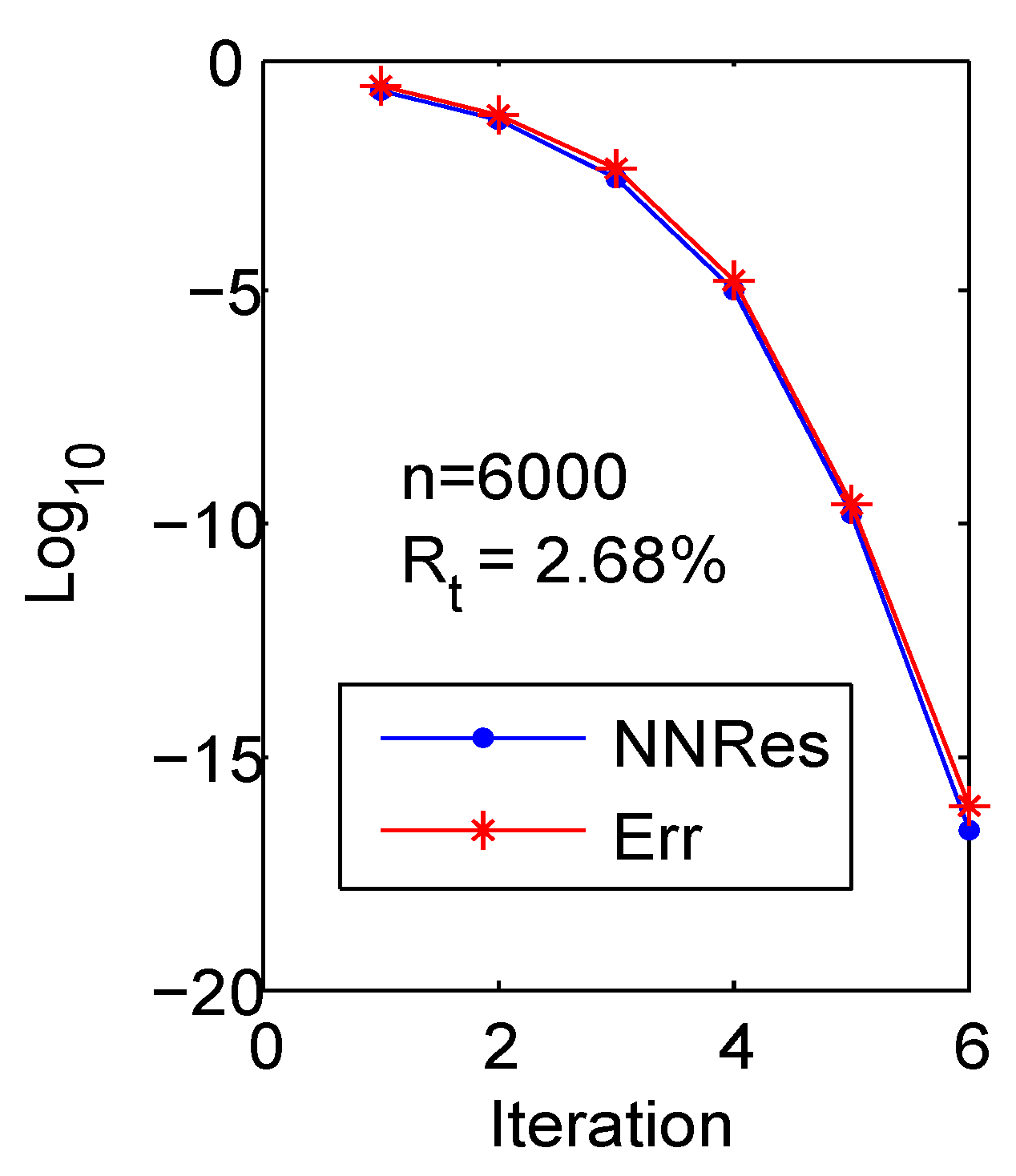
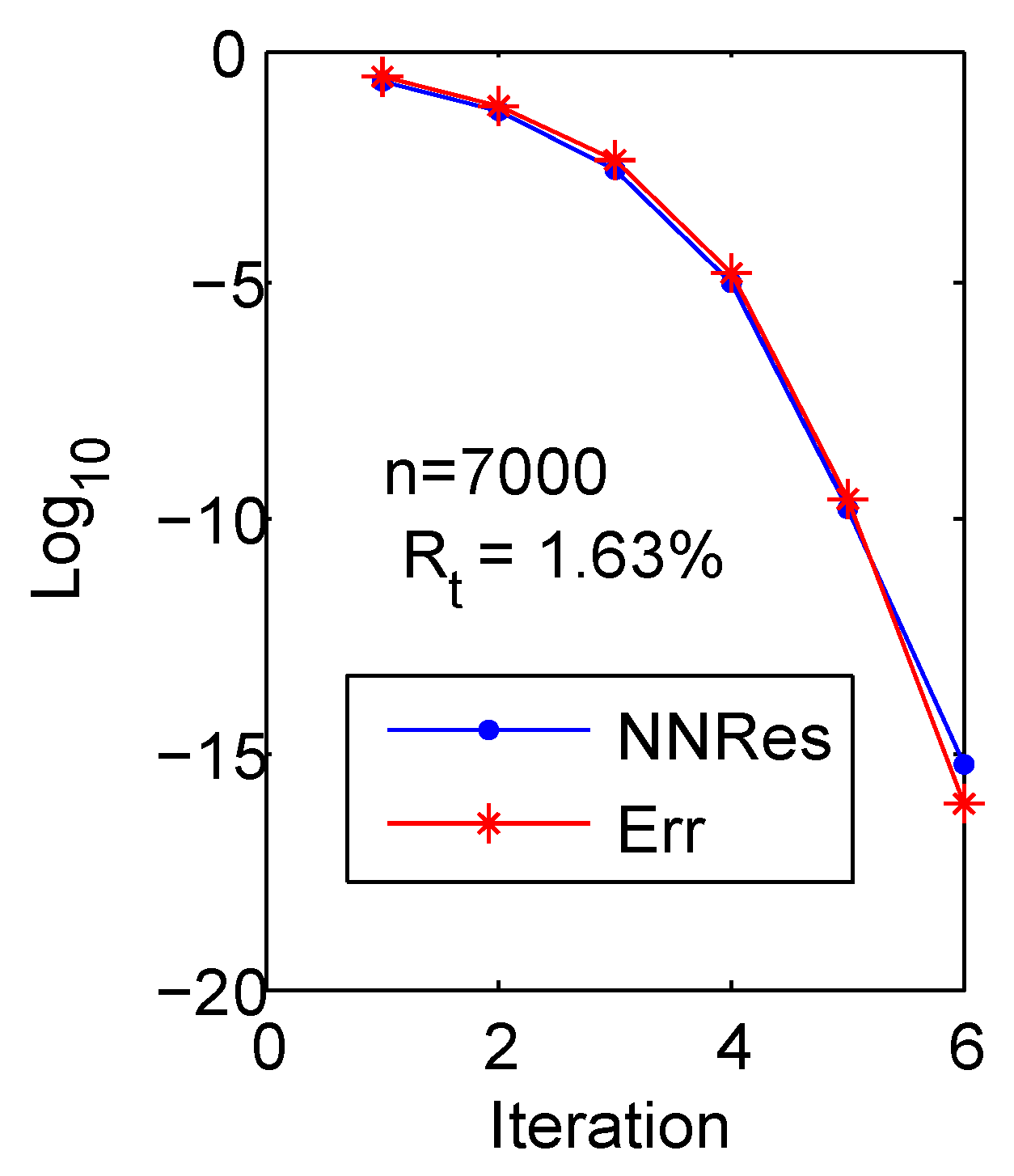
We take n = 5000 , 6000 , 7000 to test the error between the true solution and the computed solution. The obtained results together with the NRRes are plotted in Figure 1, Figure 2 and Figure 3. Still, R t represents the ratio of the iteration time and the total time.
Figure 1, Figure 2 and Figure 3 show that as the number of iterations increases, the NRRes and errors decrease exponentially and Algorithm 1 terminates at the 6th iteration. In all experiments, the preprocessing time for three cases varied from 0.1 to 0.2 s, while the iterative time only took from 0.0032 to 0.0035 s, costing a small part of the whole CPU time. More experiments also indicated that the ratio R t became smaller as the scale of the problem increased.
Example 3.
This example comes from a proper modification of the circuits from the magneto-quasistatic Maxwell equations ([17,18]). The matrix S R 632 × 632 represents the DC resistance matrix of each current filament (see Figure 4) and C 1 as well as C 2 R n × 632 associated with the mesh matrices. Let R = 1 , B = [ 1 , 0 , . . . , 0 ] R 1 × n and H = I n . We randomly generate the matrix U R n × 632 and define
U = U U 1 / 2 , C 1 = U , C 2 = U .
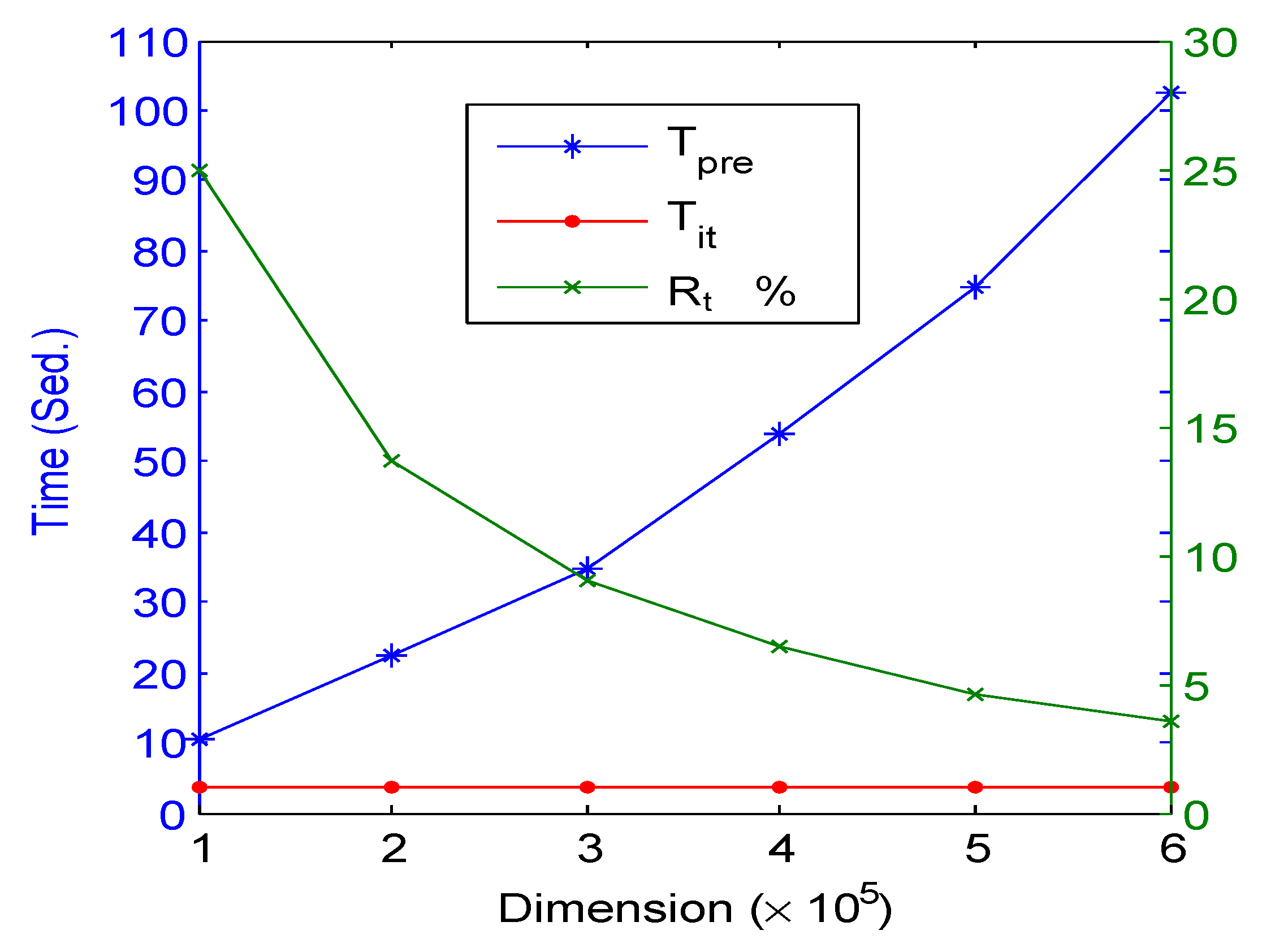
The tolerance ϵ is taken as 10 14 , and the dimensions are n = i × 10 5 ( i = 1 , 2 , . . . , 6 ).
For all cases in our experiments, Algorithm 1 was observed attaining the relative residual level below 1.01 × 10 16 at the 4-th iteration. The elapsed CPU time and the ratio R t are plotted in Figure 5, where “ T p r e ” and “ T i t ” record the CPU time for the preprocessing and for the iteration, respectively. One can see from the figure that as the scale n rises, the preprocessing time becomes more dominant (about 112 s at n = 600 , 000 ) but the iteration time remains almost unchanged (about 3.5 s for all n). The gradually reduced ratio R t also illustrates that the main computations of Algorithm 1 when solving the large-scale problems lie in the preprocessing step of O ( n ) flops, much less than the exponentially increasing one of O ( 2 k n ) in [8,9].

5. Conclusions

We have proposed an efficient algorithm to solve the large-scale DAREs with low-ranked matrices A and G and a high-rank matrix H. Compared with the SDA of the complexity O ( 2 k n ) in [8,9], the newly developed algorithm only requires preprocessing step of O ( n ) flops and iteration step of O ( ( k + 1 ) 3 m 3 ) flops. For large-scale problems with m n , the main computations of the whole algorithm lie in the preprocessing step with several matrix multiplications and an economic QR decomposition, while the elapsed CPU time for the iteration part is trivial. Some numerical experiments validate the effectiveness of the proposed algorithm. For future work, we may investigate the possibility of the SDA for solving large-scale DAREs with the structure of sparse-plus-low-rank in A, where the possible difficulty might be understanding the concrete structure of the iterative matrix and knowing how to compute and store it efficiently.

Author Contributions

Conceptualization, B.Y.; methodology, N.D.; software, C.J.; validation, B.Y.; and formal analysis, N.D. All authors have read and agreed to the final version of this manuscript.

Funding

This work was supported partly by the NSF of China (11801163), the NSF of Hunan Province (2021JJ50032, 2023JJ50040), and the Key Foundation of the Educational Department of Hunan Province (20A150).

Data Availability Statement

Not applicable.

Conflicts of Interest

The authors declare no conflict of interest.

References

  1. Athan, M.; Falb, P.L. Optimal Control: An Introduction to the Theory and Its Applications; McGraw-Hill: New York, NY, USA, 1965. [Google Scholar]
  2. Lancaster, P.; Rodman, L. Algebraic Riccati Equations; Clarendon Press: Oxford, UK, 1999. [Google Scholar]
  3. Rabbath, C.A.; Léchevin, N. Discrete-Time Control System Design with Applications; Springer Science and Business Media: Berlin/Heidelberg, Germany, 2013. [Google Scholar]
  4. Nosrati, K.; Shafiee, M. On the convergence and stability of fractional singular Kalman filter and Riccati equation. J. Frankl. Inst. 2020, 357, 7188–7210. [Google Scholar] [CrossRef]
  5. Trujillo, J.J.; Ungureanu, V.M. Optimal control of discrete-time linear fractional-order systems with multiplicative noise. Int. J. Control. 2018, 91, 57–69. [Google Scholar] [CrossRef]
  6. Chu, E.K.-W.; Fan, H.-Y.; Lin, W.-W. A structure-preserving doubling algorithm for continuous-time algebraic Riccati equations. Lin. Alg. Appl. 2005, 396, 55–80. [Google Scholar] [CrossRef]
  7. Chu, E.K.-W.; Fan, H.-Y.; Lin, W.-W.; Wang, C.-S. A structure-preserving doubling algorithm for periodic discrete-time algebraic Riccati equations. Int. J. Control 2004, 77, 767–788. [Google Scholar] [CrossRef]
  8. Chu, E.K.-W.; Weng, P.C.-Y. Large-scale discrete-time algebraic Riccati equations—Doubling algorithm and error analysis. J. Comp. Appl. Maths. 2015, 277, 115–126. [Google Scholar] [CrossRef]
  9. Yu, B.; Fan, H.-Y.; Chu, E.K.-W. Large-scale algebraic Riccati equations with high-rank constant terms. J. Comput. Appl. Math. 2019, 361, 130–143. [Google Scholar] [CrossRef]
  10. Kamon, M.; Wang, F.; White, J. Generating nearly optimally compact models from Krylov-subspace based reduced order models. IEEE Trans. Circuits -Syst.-Ii Analog Digit. Signal Process. 2000, 47, 239–248. [Google Scholar] [CrossRef]
  11. Golub, G.H.; Van Loan, C.F. Matrix Computations, 3rd ed.; Johns Hopkins University Press: Baltimore, MD, USA, 1996. [Google Scholar]
  12. Yu, B.; Li, D.-H.; Dong, N. Low memory and low complexity iterative schemes for a nonsymmetric algebraic Riccati equation arising from transport theory. J. Comput. Appl. Math. 2013, 250, 175–189. [Google Scholar] [CrossRef]
  13. Lin, W.-W.; Xu, S.-F. Convergence analysis of structure-preserving doubling algorithms for Riccati-type matrix equations. SIAM J. Matrix Anal. Appl. 2006, 28, 26–39. [Google Scholar] [CrossRef]
  14. Bhatia, R. Matrix Analysis, Graduate Texts in Mathematics; Springer: Berlin/Heidelberg, Germany, 1997. [Google Scholar]
  15. Higham, N.J. Functions of Matrices: Theory and Computation; SIAM: Philadelphia, PA, USA, 2008. [Google Scholar]
  16. Higham, D.J.; Higham, N.J. MATLAB Guide; Society for Industrial and Applied Mathematics: Philadelphia, PA, USA, 2016. [Google Scholar]
  17. Miguel, S.L.; Kamon, M.; Elfadel, I.; White, J. A coordinate transformed Arnoldi algorithm for generating guaranteed stable reduced order models of RLC circuits. In Proceedings of the IEEE/ACM International Conference on Computer-Aided Design, San Jose, CA, USA, 10–14 November 1996; pp. 288–294. [Google Scholar]
  18. Odabasioglu, A.; Celik, M.; Pileggi, L.T. PRIMA: Passive Reduced order Interconnect Macro modeling Algorithm. IEEE Trans.-Comput.-Aided Des. Integr. Circuits Syst. 1998, 17, 645–654. [Google Scholar] [CrossRef] [Green Version]
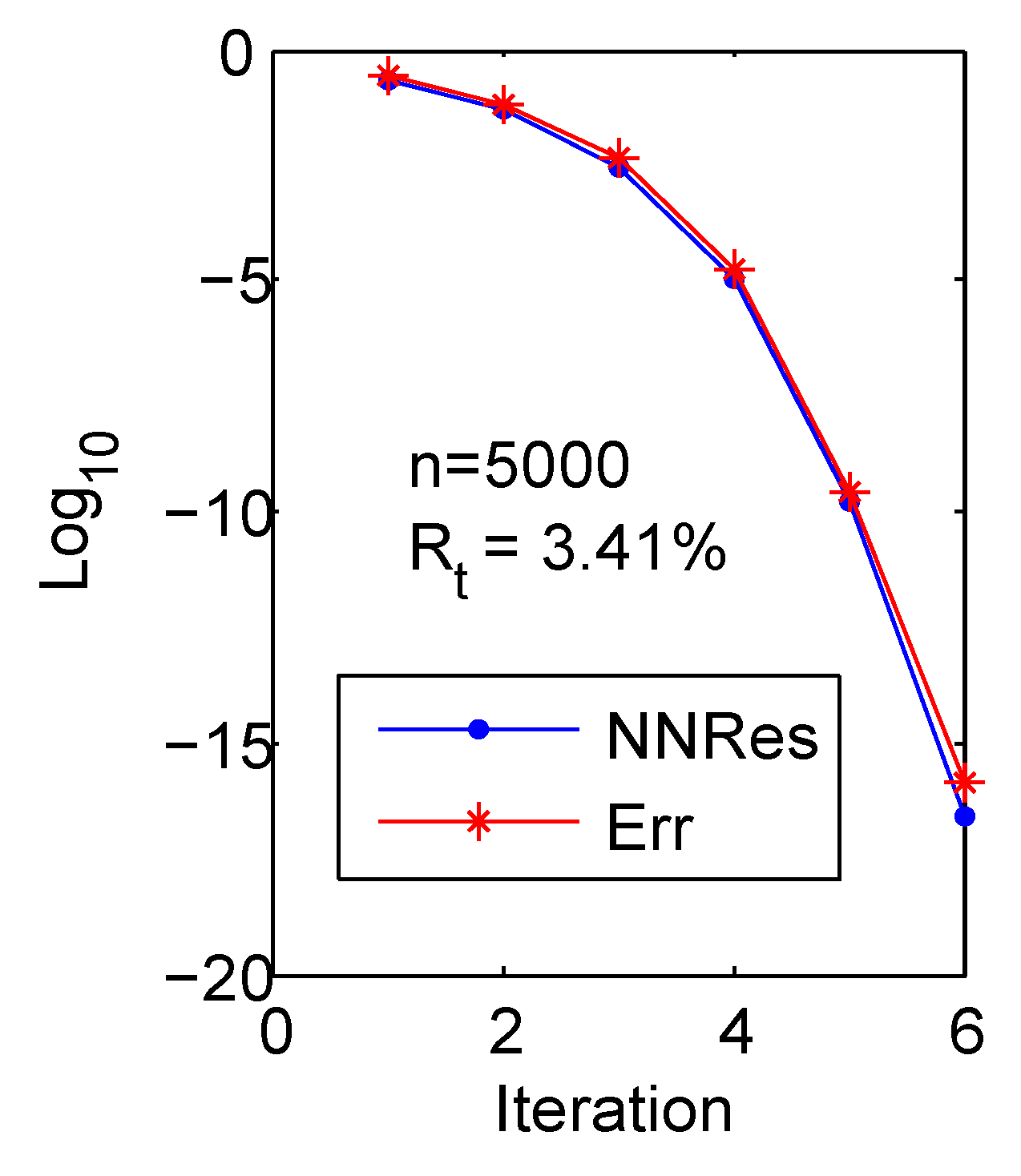
Figure 1. History of NRRes and Error for n = 5000 in Example 2.
Fractalfract 07 00193 g001
Figure 2. History of NRRes and Error for n = 6000 in Example 2.
Fractalfract 07 00193 g002
Figure 3. History of NRRes and Error for n = 7000 in Example 2.
Fractalfract 07 00193 g003
Figure 4. The structure of the DC resistance matrix of each current filament.
Fractalfract 07 00193 g004
Figure 5. Preprocessing time ( T pre ), iteration time ( T it ), and R t for different dimensions in Example 3.
Fractalfract 07 00193 g005
Table 1. Complexity and memory of the preprocessing step in Algorithm 1.
ItemsFlopsMemory
H C 1 , H B 2 m ( m + l ) n ( m + l ) n
C 1 * H C 1 , C 1 * H B , B * H B 2 ( m 2 + m l + l 2 ) n m 2 + m l + l 2
C 2 * C 1 , C 2 * B 2 m ( m + l ) n m 2 + m l
C 2 = Q C 2 R C 2 ( 10 m 2 + 4 m l + 4 l 2 ) n m 2
Total ( 16 m 2 + 10 m l + 6 l 2 ) n 3 m 2 + 2 m l + l 2 + ( m + l ) n
Table 2. Complexity and memory at kth iteration in Algorithm 1.
ItemsFlopsMemory
Σ k 1 Φ k * , Σ k 1 Ψ k * 16 ( k m + l ) 2 m 2 ( k m + l ) m
Φ k * Σ k 1 Ψ k * , Φ k * Σ k 1 Φ k * , Ψ k * Σ k 1 Ψ k * 6 m 2 ( k m + l ) 3 m 2
S k + 1 4 m 3 m 2
T k + 1 8 m 3 m 2
R k + 1 4 m 3 m 2
B k + 1 * H k + 1 B k + 1 2 m ( 2 m 2 + 2 m l + l 2 ) ( ( k + 1 ) m + l ) 2
Σ k + 1 2 ( ( k + 1 ) m ) 3 ( ( k + 1 ) m ) 2
Φ k + 1 ( ( k + 1 ) m + l ) m
Ψ k + 1 4 m 2 ( m + l ) ( ( k + 1 ) m + l ) m
Total ( 24 + 2 ( k + 1 ) 3 ) m 3 + 2 m l ( 4 m + l ) + 2 m ( k m + l ) ( 8 ( k m + l ) + 3 m ) ( 4 ( k + 1 ) 2 + 2 k + 6 ) m 2 + ( 2 k + 6 ) m l + l 2
Table 3. Residual and actual errors in Example 1.
n100030005000
NRRes 1 9.99 × 10 1 9.99 × 10 1 9.99 × 10 1
NRRes 2 2.49 × 10 7 2.77 × 10 7 9.99 × 10 8
NRRes 3 6.24 × 10 17 3.62 × 10 17 4.48 × 10 18
H 1 X 9.99 × 10 1 9.99 × 10 1 9.99 × 10 1
H 2 X 2.26 × 10 7 3.33 × 10 7 2.75 × 10 7
H 3 X 1.24 × 10 14 1.25 × 10 14 1.24 × 10 14
R t 37.5 % 12.6 % 6.8 %
Disclaimer/Publisher’s Note: The statements, opinions and data contained in all publications are solely those of the individual author(s) and contributor(s) and not of MDPI and/or the editor(s). MDPI and/or the editor(s) disclaim responsibility for any injury to people or property resulting from any ideas, methods, instructions or products referred to in the content.