New Complex Wave Solutions and Diverse Wave Structures of the (2+1)-Dimensional Asymmetric Nizhnik–Novikov–Veselov Equation

Abstract

In this paper, we use a new, extended Jacobian elliptic function expansion method to explore the exact solutions of the (2+1)-dimensional asymmetric Nizhnik–Novikov–Veselov (aNNV) equation, which is a nonlinear physical model to describe an incompressible fluid. Combined with the mapping method, many new types of exact Jacobian elliptic function solutions are obtained. As we use two new forms of transformation, most of the solutions obtained are not found in previous studies. To show the complex nonlinear wave phenomena, we also provide various wave structures of a group of solutions, including periodic wave and solitary wave structures of ordinary traveling wave solutions, horseshoe-type wave, s-type wave and breaker-wave structures superposed by two kinds of waves: chaotic wave structures with chaotic behavior and spiral wave structures. The results show that this method is effective and powerful and can be used to construct various exact solutions for a wide range of nonlinear models and complex nonlinear wave phenomena in mathematical and physical research.

1. Introduction

Nonlinear problems widely existing in the fields of natural science and social science have attracted more and more attention, and many nonlinear discrimination problems can be described by nonlinear evolution equations (NLEEs). In modern physics and engineering, many famous NLEEs have been developed to explain the dynamics of nonlinear waves [1,2,3,4,5,6]. Therefore, obtaining their exact solutions is very important for researching related nonlinear problems, and this is a core issue in mathematics and physics [7,8,9,10,11,12,13]. In recent years, significant progress has been made and many powerful and effective methods have been developed to obtain the exact solution for NLEEs. For example, the sine–cosine method [14], modified extended direct algebraic method [15], homogeneous balance method [16], F-expansion method [17,18], tanh-sech method and the extended tanh–coth method [19,20], Exp function method [21], Jacobi elliptic function expansion method [22,23], the modified, extended mapping method [24,25,26], the auxiliary equation method [27,28,29], and so on. In this paper, we consider exploring the new exact solutions of the following (2+1)-dimensional aNNV system [30,31]:

$$u_t+u_{xxx} – 3v_{x}u – 3v{u}_x=0,$$

(1)

$$u_x=v_y,$$

(2)

If v = u and y = x, the above formulas degenerate into the (1+1)-dimensional Korteweg-de Vries (KDV) equation. The (2+1)-dimensional case involves more complex nonlinear phenomena, which can describe some physical phenomena in plasmas and fluids. U(x, y, t) and v(x, y, t) are real differential wave functions, which depend on the two-dimensional space variable x and y and the one-dimensional time variable t. Equations (1) and (2) were solved in different methods. The variable separation solution of Equations (1) and (2) was obtained in Refs. [32,33], and some types of solitary wave solutions were given in Ref. [34]. Multi-solitons, breather solutions, lump soliton, lump-kink waves and multi-lumps are obtained by applying the bilinear form in Ref. [35]. Abundant periodic wave solutions are given in Ref. [36] through an extended F-expansion method. Ref. [37] constructs a large number of Jacobi elliptic function solutions and Weierstrass elliptic function solutions by using the bifurcation theory of the planar dynamic system. Ref. [38] applies the sine–cosine and tanh–coth methods to obtain many stochastic exact solutions for the stochastic (2+1)-dimensional NNV system. Although these methods are effective in solving the (2+1)-dimensional aNNV equation, there are still some new types of solutions to be explored. In all the methods, because the elliptic Jacobian function includes trigonometric function and hyperbolic function under limited conditions, and the elliptic equation has good constructivity, it is widely used in solving NLEEs. The early Jacobian elliptic function expansion method can only construct simple Jacobian elliptic function solutions [22,23]. Refs. [27,36] can construct complex Jacobian elliptic function solutions through the extended F-expansion method. The main purpose of this work is to develop two new functional transformations of the Jacobian elliptic equation that have not been reported in other documents to construct abundant arbitrary wave solutions of (2+1)-dimensional aNNV system. Through these two new transformations, we obtain a large number of new Jacobian elliptic function type arbitrary wave solutions of the (2+1)-dimensional aNNV system, most of which are new ones that have not been found in previous studies.

Furthermore, we have discussed some new nonlinear wave phenomena, such as periodic waves and solitary waves. Since an arbitrary wave is a wave structure that can be constructed arbitrarily, we have also discussed the complex wave phenomena of two kinds of periodic wave superposition and periodic wave and solitary wave superposition. In order to explore the more complex nonlinear wave phenomena of the (2+1)-dimensional aNNV system, we have also constructed the chaotic wave solutions and spiral wave solutions. The numerical simulation shows the complex wave behavior of (2+1)-dimensional aNNV system under these two nonlinear wave states. The method we used can greatly extend the earlier Jacobi elliptic function expansion method and the F-expansion method. At the same time, our method can also simplify the process of solving NLEEs and construct a large number of new types of exact solutions and diverse nonlinear wave phenomena.

The manuscript is organized as follows. In Section 2, the new Jacobian elliptic function solutions are constructed, which provides abundant, exact solutions. This part is the theoretical basis of this paper. In Section 3, the main steps of the scheme are described in detail to (2+1)-dimensional aNNV system. In Section 4, we give a demonstration of a group of Jacobian elliptic function solutions, which proves that our method is powerful and effective. The complex nonlinear wave phenomena are shown in Section 5. Finally, the conclusion and discussion are given in Section 6.

2. Solutions of Elliptic Jacobian Equation

Jacobi elliptic equation is generally expressed as follows:

$${\left[g^{\prime }\left(\xi \right)\right]}^2=p{g}^4\left(\xi \right)+q{g}^2\left(\xi \right)+r,$$

(3)

where p, q and r are parameters of the Jacobi elliptic function. In Ref. [27], by selecting different p, q and r, the Jacobi elliptic function solutions of Equation (3) are shown in

Table 1. The mapping of the Jacobi elliptic function solutions for Equation (3).

$\mathit{g}\left(\mathit{\xi }\right)$	$\mathit{p}$	$\mathit{q}$	$\mathit{r}$
$sn\left(\xi \right), cd\left(\xi \right)=cn\left(\xi \right)/dn\left(\xi \right)$	$m^2$	$-\left(1+m^2\right)$	$1$
$cn\left(\xi \right)$	$-m^2$	$-1+2m^2$	$1-m^2$
$dn\left(\xi \right)$	$-1$	$2-m^2$	$-1+m^2$
$\begin{array}{c}ns\left(\xi \right)=\frac{1}{sn\left(\xi \right)},\\ dc\left(\xi \right)=dn\left(\xi \right)/cn\left(\xi \right)\end{array}$	$1$	$-\left(1+m^2\right)$	$m^2$
$nc\left(\xi \right)=1/ cn\left(\xi \right)$	$1-m^2$	$-1+2m^2$	$-m^2$
$nd\left(\xi \right)=1/ dn\left(\xi \right)$	$-1+m^2$	$2-m^2$	$-1$
$cs\left(\xi \right)=cn\left(\xi \right)/sn\left(\xi \right)$	$1$	$2-m^2$	$1-m^2$
$sc\left(\xi \right)=sn\left(\xi \right)/cn\left(\xi \right)$	$1-m^2$	$2-m^2$	$1$
$sd\left(\xi \right)=sn\left(\xi \right)/dn\left(\xi \right)$	$m^2\left(-1+m^2\right)$	$-1+2m^2$	$1$
$ds\left(\xi \right)=dn\left(\xi \right)/sn\left(\xi \right)$	$1$	$-1+2m^2$	$m^2\left(-1+m^2\right)$
$m cn\left(\xi \right)\pm dn\left(\xi \right)$	$-1/4$	$\left(1+m^2\right)/2$	$-{\left(1-m^2\right)}^2/4$
$\begin{array}{c}ns\left(\xi \right)\pm cs\left(\xi \right),\\ cn\left(\xi \right)/(\sqrt{1-m^2}sn\left(\xi \right)\pm dn\left(\xi \right)\\ msn\left(\xi \right)\pm idn\left(\xi \right),\\ sn\left(\xi \right)/(1\pm cn\left(\xi \right)\end{array}$	$1/4$	$\left(1-2m^2\right)/2$	$1/4$
$nc\left(\xi \right)\pm sc\left(\xi \right), cn\left(\xi \right)/\left(1\pm sn\left(\xi \right)\right)$	$\left(1-m^2\right)/4$	$\left(1+m^2\right)/2$	$\left(1-m^2\right)/4$
$ns\left(\xi \right)\pm ds\left(\xi \right)$	$1/4$	$\left(-2+m^2\right)/2$	$m^4/4$
$\begin{array}{c}sn\left(\xi \right)\pm icn\left(\xi \right),\\ dn\left(\xi \right)/\left(\sqrt{m^2-1}sn\left(\xi \right)\pm cn\left(\xi \right)\right)\end{array}$	$m^2/4$	$\left(-2+m^2\right)/2$	$m^2/4$
$dn\left(\xi \right)/\left(\sqrt{\frac{m^2-1}{m^2}}\pm cn\left(\xi \right)\right)$	$\frac{1}{4m^2}$	$\left(1-2m^2\right)/2$	$m^2/4$
$sn\left(\xi \right)/\left(1\pm dn\left(\xi \right)\right)$	$m^2/4$	$\left(-2+m^2\right)/2$	$1/4$
$dn\left(\xi \right)/\left(1\pm msn\left(\xi \right)\right)$	$\left(-1+m^2\right)/4$	$\left(1+m^2\right)/2$	$\left(-1+m^2\right)/4$
$sn\left(\xi \right)/\left( cn\left(\xi \right)\pm dn\left(\xi \right)\right)$	${\left(1-m^2\right)}^2/4$	$\left(1+m^2\right)/2$	$1/4$
$cn\left(\xi \right)/\left(\sqrt{1-m^2}\pm dn\left(\xi \right)\right)$	$m^4/4$	$\left(-2+m^2\right)/2$	$1/4$
$sn\left(\xi \right)/\left( cn\left(\xi \right)dn\left(\xi \right)\right)$	${\left(1-m^2\right)}^2$	$2\left(1+m^2\right)$	$1$
$cn\left(\xi \right)dn\left(\xi \right)/ sn\left(\xi \right)$	$1$	$2\left(1+m^2\right)$	${\left(1-m^2\right)}^2$
$\begin{array}{c}\frac{\mathrm{cn}\left(\mathsf{\xi }\right)}{\mathrm{sn}\left(\mathsf{\xi }\right)\mathrm{dn}\left(\mathsf{\xi }\right)},\\ \mathrm{sn}\left(\mathsf{\xi }\right)\mathrm{dn}\left(\mathsf{\xi }\right)/\mathrm{cn}\left(\mathsf{\xi }\right)\end{array}$	$1$	$2\left(1-2m^2\right)$	$1$
$sn\left(\xi \right)cn\left(\xi \right)/dn\left(\xi \right)$	$m^4$	$2\left(-2+m^2\right)$	$1$
$dn\left(\xi \right)/\left(sn\left(\xi \right)cn\left(\xi \right)\right)$	$1$	$2\left(-2+m^2\right)$	$m^4$

where i² = −1.

To find new forms of Jacobian elliptic function solutions, we introduce another Jacobian elliptic equation:

$${\left[f^{\prime }\left(\xi \right)\right]}^2=p_1{f}^4\left(\xi \right)+q_1{f}^2\left(\xi \right)+r_1,$$

(4)

where p₁, q₁, and r₁ are parameters to be determined. To solve Equation (4), we first assume that it has the following formal solution:

Case 1

$$f\left(\xi \right)=g\left(\xi \right)+\mu \frac{1}{g\left(\xi \right)},$$

(5)

where μ is a constant. Substituting Equation (5) into (4), and setting the coefficients of gⁱ(ξ) to zero yields a set of algebraic equations for p₁, q₁, r₁ and μ. Solving the algebraic equations, p₁, q₁, r₁ and μ can be expressed as:

$$p_1=p, q_1=q\pm 6\sqrt{pr}, r_1=8r\pm 4q\sqrt{\frac{r}{p}}, \mu =\mp \sqrt{\frac{r}{p}}.$$

(6)

Through this function transformation, f (ξ) is transformed into the Jacobian elliptic function solutions represented by g(ξ).

We again assume that Equation (4) has the following form solution:

Case 2

$$f\left(\xi \right)=\sqrt{a{g}^2\left(\xi \right)+b{g}^{\prime }\left(\xi \right)+c}.$$

(7)

By solving this case, we can obtain:

Solutions 1

$$a=\pm b\sqrt{p},c=\pm \frac{bq}{2\sqrt{p}}, p_1=\pm \frac{\sqrt{p}}{2b}, q_1=-\frac{q}{2}, r_1=\pm \frac{\left(q^2-4pr\right)b}{8\sqrt{p}}, b\ne 0.$$

(8)

Solutions 2

$$a=\pm b\sqrt{p},c=-b\sqrt{r}, p_1=\pm \frac{\sqrt{p}}{2b}, q_1=\frac{1}{4}\left(q\pm 6\sqrt{pr}\right), r_1=\frac{\left(q\sqrt{r}\pm 2r\sqrt{p}\right)b}{2}, b\ne 0.$$

(9)

Through Equations (4)–(9) and Table 1, we have constructed abundant and diverse Jacobian elliptic function solutions of the Jacobian elliptic equation. Many of these solutions have not been found in previous studies, especially the solution represented by Equation (7).

3. Method and Application to the (2+1)-Dimensional aNNV Equation

We assume Equation (1) and Equation (2) have the following arbitrary wave solution:

$$u\left(x,y,t\right)=u\left(\xi \right), v\left(x,y,t\right)=v\left(\xi \right), \xi =kx+\mathsf{\Phi }\left(y,t\right)+\psi \left(t\right),$$

(10)

where k is a constant to be determined, $\mathsf{\Phi }\left(y,t\right)$ is an arbitrary wave function about y and t, and $\psi \left(t\right)$ is an arbitrary function about t. When the Jacobian elliptic equation method is used to solve (2+1)-dimensional aNNV system, the arbitrary wave function for x does not exist, so we adopt arbitrary wave transformation shown in Equation (10). Substituting Equation (10) into Equation (1) and Equation (2) and integrating once, and setting the integration constant to zero yields:

$$({\mathsf{\Phi }}_t+{\psi }_t)u\prime -3k{v}^{\prime }u-3kvu\prime +k^{3}v″=0,$$

(11)

$$ku\prime ={\mathsf{\Phi }}_{y}v\prime ,$$

(12)

where $u^{\prime }$, $v\prime$, ${\psi }_t$, ${\mathsf{\Phi }}_t$ and ${\mathsf{\Phi }}_y$ mean $\frac{du\left(\xi \right)}{d\xi }$, $\frac{dv\left(\xi \right)}{d\xi }$, $\frac{\partial \psi \left(t\right)}{\partial t}$, $\frac{\partial \mathsf{\Phi }\left(\mathrm{y},\mathrm{t}\right)}{\partial t}$ and $\frac{\partial \mathsf{\Phi }\left(\mathrm{y},\mathrm{t}\right)}{\partial y}$. Then, according to the method in Ref. [27], we assume Equations (11) and (12) have the following formal solutions:

$$u\left(x, y,t\right)=a_0+a_{1}f\left(\xi \right)+b_1\frac{1}{f\left(\xi \right)}+c_1\frac{f^{\prime }\left(\xi \right)}{f\left(\xi \right)}+a_2{f}^2\left(\xi \right)+b_2\frac{1}{f^2\left(\xi \right)}+c_2\frac{f^{\prime }\left(\xi \right)}{f^2\left(\xi \right)}+d_2{f}^{\prime }\left(\xi \right),$$

(13)

$$v\left(x, y,t\right)=A_0+A_{1}f\left(\xi \right)+B_1\frac{1}{f\left(\xi \right)}+C_1\frac{f^{\prime }\left(\xi \right)}{f\left(\xi \right)}+A_2{f}^2\left(\xi \right)+B_2\frac{1}{f^2\left(\xi \right)}+C_2\frac{f^{\prime }\left(\xi \right)}{f^2\left(\xi \right)}+D_2{f}^{\prime }\left(\xi \right),$$

(14)

where a_i, b_i, c_i, d_i, A_i, B_i, C_i and D_i are constants determined later, f (ξ) represents the solutions of Equation (4). By substituting Equations (13) and (14) into Equations (11) and (12) and setting the coefficients of $f^i\left(\xi \right)$ and $f^i\left(\xi \right)f^{\prime }\left(\xi \right)$ to zero yields, a set of algebraic equations a_i, b_i, c_i, d_i, A_i, B_i, C_i, D_i, ${\mathsf{\Phi }}_t$, ${\psi }_t$ and k. Solving the resulting equations, the following coefficients can be obtained:

Set 1

$$\begin{gathered} a_0=\frac{\left(4k^3{q}_1+{\mathsf{\Phi }}_t+{\psi }_t\right){\mathsf{\Phi }}_y}{6k^2}, a_1=b_1=c_1=b_2=c_2=d_2=A_1=B_1=C_1=B_2=C_2=C_2=0, \\ {A}_0=\frac{4k^3{q}_1+{\mathsf{\Phi }}_t+{\psi }_t}{6k}, a_2=2k{p}_1{\mathsf{\Phi }}_y, A_2=2k^2{p}_1,{\mathsf{\Phi }}_t+{\psi }_t=\pm 4k^3\sqrt{q_1{}^2-3p_1{r}_1}. \end{gathered}$$

(15)

Set 2

$$\begin{gathered} a_0=\frac{\left(4k^3{q}_1+{\mathsf{\Phi }}_t+{\psi }_t\right){\mathsf{\Phi }}_y}{6k^2}, a_1=b_1=c_1=a_2=c_2=d_2=A_1=B_1=C_1=A_2=C_2=D_2=0, \\ {A}_0=\frac{4k^3{q}_1+{\mathsf{\Phi }}_t+{\psi }_t}{6k}, b_2=2k{r}_1{\mathsf{\Phi }}_y,B_2=2k^2{r}_1, {\mathsf{\Phi }}_t+{\psi }_t=\pm 4k^3\sqrt{q_1{}^2-3p_1{r}_1}. \end{gathered}$$

(16)

Set 3

$$\begin{gathered} a_0=\frac{(k^3{q}_1+{\mathsf{\Phi }}_t+{\psi }_t){\mathsf{\Phi }}_y}{6k^2}, a_1=b_1=c_1=b_2=c_2=A_1=B_1=C_1=B_2=C_2=0, A_0=\frac{k^3{q}_1+{\mathsf{\Phi }}_t+{\psi }_t}{6k}, \\ a_2=k{p}_1{\mathsf{\Phi }}_y, d_2=\pm k{\mathsf{\Phi }}_y\sqrt{p_1 }, A_2=k^2{p}_1, D_2=\pm k^2\sqrt{p_1 },{\mathsf{\Phi }}_t+{\psi }_t=k^3\sqrt{q_1{}^2+12p_1{r}_1}. \end{gathered}$$

(17)

Set 4

$$\begin{gathered} a_0=\frac{(k^3{q}_1+{\mathsf{\Phi }}_t+{\psi }_t){\mathsf{\Phi }}_y}{6k^2}, a_1=b_1=c_1=a_2=d_2=A_1=B_1=C_1=A_2=D_2=0,A_0=\frac{k^3{q}_1+{\mathsf{\Phi }}_t+{\psi }_t}{6k}, \\ b_2=k{\mathsf{\Phi }}_y{r}_1, c_2=\pm k{\mathsf{\Phi }}_y\sqrt{r_1 }, B_2=k^2{r}_1, C_2=\pm k^2\sqrt{r_1 },{\mathsf{\Phi }}_t+{\psi }_t{k}^3\sqrt{q_1{}^2+12p_1{r}_1}. \end{gathered}$$

(18)

Set 5

$$\begin{gathered} a_0=\frac{(k^3{q}_1\pm 6k^3\sqrt{p_1{r}_1}+{\mathsf{\Phi }}_t+{\psi }_t){\mathsf{\Phi }}_y}{6k^2},a_1=b_1=c_1=A_1=B_1=C_1=0,a_2=k{p}_1{\mathsf{\Phi }}_y, \\ {b}_2=k{r}_1{\mathsf{\Phi }}_y, c_2=\pm k{\mathsf{\Phi }}_y\sqrt{r_1 },d_2= \pm k{\mathsf{\Phi }}_y\sqrt{p_1 }, A_2=k^2{p}_1,B_2=2k^2{r}_1, C_2=\pm k^2\sqrt{r_1 }, \\ {D}_2=\pm k^2\sqrt{p_1 },{ \mathsf{\Phi }}_t+{\psi }_t=\pm k^3\sqrt{q_1{}^2+132p_1{r}_1\pm 60q_1\sqrt{p_1{r}_1}}. \end{gathered}$$

(19)

Therefore, according to all the above sets, the solutions of Equations (11) and (12) read

$$u_1\left(x, y,t\right)=\frac{\left(4k^3{q}_1+{\mathsf{\Phi }}_t+{\psi }_t\right){\mathsf{\Phi }}_y}{6k^2}+2k{p}_1{\mathsf{\Phi }}_y{f}^2\left(\xi \right),$$

(20)

$$v_1\left(x, y,t\right)=\frac{4k^3{q}_1+{\mathsf{\Phi }}_t+{\psi }_t}{6k}+2k^2{p}_1{f}^2\left(\xi \right),$$

(21)

where $\xi =kx+\mathsf{\Phi }\left(y,t\right)+\psi \left(t\right), k\ne 0$,${ \mathsf{\Phi }}_t+{\psi }_t=\pm 4k^3\sqrt{q_1{}^2-3p_1{r}_1}$.

$$u_2\left(x, y,t\right)=\frac{\left(4k^3{q}_1+{\mathsf{\Phi }}_t+{\psi }_t\right){\mathsf{\Phi }}_y}{6k^2}+2k{r}_1{\mathsf{\Phi }}_y\frac{1}{f^2\left(\xi \right)},$$

(22)

$$v_2\left(x, y,t\right)=\frac{4k^3{q}_1+{\mathsf{\Phi }}_t+{\psi }_t}{6k}+2k^2{r}_1\frac{1}{f^2\left(\xi \right)},$$

(23)

where $\xi =kx+\mathsf{\Phi }\left(y,t\right)+\psi \left(t\right),k\ne 0$,${ \mathsf{\Phi }}_t+{\psi }_t=\pm 4k^3\sqrt{q_1{}^2-3p_1{r}_1}$.

$$u_3\left(x, y,t\right)=\frac{\left(k^3{q}_1+{\mathsf{\Phi }}_t+{\psi }_t\right){\mathsf{\Phi }}_y}{6k^2}+k{p}_1{\mathsf{\Phi }}_y{f}^2\left(\xi \right)\pm k{\mathsf{\Phi }}_y\sqrt{p_1}{f}^{\prime }\left(\xi \right),$$

(24)

$$v_3\left(x, y,t\right)=\frac{k^3{q}_1+{\mathsf{\Phi }}_t+{\psi }_t}{6k}+k^2{p}_1{f}^2\left(\xi \right)\pm k^2\sqrt{p_1}{f}^{\prime }\left(\xi \right),$$

(25)

where $\xi =kx+\mathsf{\Phi }\left(y,t\right)+\psi \left(t\right), k\ne 0,{\mathsf{\Phi }}_t+{\psi }_t=k^3\sqrt{q_1{}^2+12p_1{r}_1}$.

$$u_4\left(x, y,t\right)=\frac{(k^3{q}_1+{\mathsf{\Phi }}_t+{\psi }_t){\mathsf{\Phi }}_y}{6k^2}+k{r}_1{\mathsf{\Phi }}_y\frac{1}{f^2\left(\xi \right)}\pm k{\mathsf{\Phi }}_y\sqrt{r_1}\frac{f^{\prime }\left(\xi \right)}{f^2\left(\xi \right)},$$

(26)

$$v_4\left(x, y,t\right)=\frac{k^3{q}_1+{\mathsf{\Phi }}_t+{\psi }_t}{6k}+k^2{r}_1\frac{1}{f^2\left(\xi \right)}\pm k^2\sqrt{r_1}\frac{f^{\prime }\left(\xi \right)}{f^2\left(\xi \right)},$$

(27)

where $\xi =kx+\mathsf{\Phi }\left(y,t\right)+\psi \left(t\right), k\ne 0,{\mathsf{\Phi }}_t+{\psi }_t=k^3\sqrt{q_1{}^2+12p_1{r}_1}$.

$$u_5\left(x, y,t\right)=\frac{(k^3{q}_1\pm 6k^3\sqrt{p_1{r}_1}+{\mathsf{\Phi }}_t+{\psi }_t){\mathsf{\Phi }}_y}{6k^2}+k{p}_1{\mathsf{\Phi }}_y{f}^2\left(\xi \right)+k{r}_1{\mathsf{\Phi }}_y\frac{1}{f^2\left(\xi \right)}\pm k{\mathsf{\Phi }}_y\sqrt{p_1}{f}^{\prime }\left(\xi \right)\pm k{\mathsf{\Phi }}_y\sqrt{r_1}\frac{f^{\prime }\left(\xi \right)}{f^2\left(\xi \right)},$$

(28)

$$v_5\left(x, y,t\right)=\frac{k^3{q}_1\pm 6k^3\sqrt{p_1{r}_1}+{\mathsf{\Phi }}_t+{\psi }_t}{6k}+k^2{p}_1{f}^2\left(\xi \right)+k^2{r}_1\frac{1}{f^2\left(\xi \right)}\pm k^2\sqrt{p_1}{f}^{\prime }\left(\xi \right)\pm k^2\sqrt{r_1}\frac{f^{\prime }\left(\xi \right)}{f^2\left(\xi \right)},$$

(29)

where $\xi =kx+\mathsf{\Phi }\left(y,t\right)+\psi \left(t\right), k\ne 0,{\mathsf{\Phi }}_t+{\psi }_t=\pm k^3\sqrt{q_1{}^2+132p_1{r}_1\pm 60q_1\sqrt{p_1{r}_1}}$.

Using Equations (3)–(9), p₁, q₁ and r₁ can be transformed into the expressions of p, q and r. Then looking up the elliptic Jacobian function corresponding to p, q and r from Table 1, the exact solutions of the (2+1)-dimensional aNNV equation can be obtained. These are five sets of solutions containing many Jacobi elliptic functions, hyperbolic function solutions when m → 1 and trigonometric function solutions when m → 0. They are basically new types of solutions that have not been found in other documents due to the new function transformations in Equations (5) and (7).

4. Demonstration of the Solutions

An example will be given in the following to demonstrate the power and effectiveness of this method. If $p=m^2$, $q=-\left(1+m^2\right)$ and $r=1$, $g\left(\xi \right)=sn\left(\xi \right)$, we have:

Case 1

$$p_1=m^2, q_1=-\left(1+m^2\right)\pm 6m, r_1=8\mp 4\left(1+m^2\right)/m, \mu =\mp \frac{1}{m}.$$

(30)

Case 2

Solutions 1

$$a=\pm bm,c=\mp \frac{b\left(1+m^2\right)}{2m}, p_1=\pm \frac{m}{2b}, q_1=\frac{1+m^2}{2}, r_1=\pm \frac{{\left(1-m^2\right)}^{2}b}{8m}, b\ne 0.$$

(31)

Solutions 2

$$a=\pm bm,c=-b, p_1=\pm \frac{m}{2b}, q_1=\frac{1}{4}\left(-1-m^2\pm 6m\right), r_1=\frac{\left[-\left(1+m^2\right)\pm 2m\right]b}{2}, b\ne 0.$$

(32)

Substituting Equations (30)–(32) into Equations (21)–(30), according to Case 1, we have the following Jacobian elliptic function solutions of the (2+1)-dimensional aNNV equation are shown as:

$$u_{11}\left(x, y,t\right)=\frac{\left[4k^3\left(-1-m^2\right)+{\mathsf{\Phi }}_t+{\psi }_t\right]{\mathsf{\Phi }}_y}{6k^2}+2m^{2}k{\mathsf{\Phi }}_y\left[s{n}^2\left(\xi \right)+\frac{1}{m^{2}s{n}^2\left(\xi \right)}\right],$$

(33)

$$v_{11}\left(x, y,t\right)=\frac{4k^3\left(-1-m^2\right)+{\mathsf{\Phi }}_t+{\psi }_t}{6k}+2m^2{k}^2\left[s{n}^2\left(\xi \right)+\frac{1}{m^{2}s{n}^2\left(\xi \right)}\right],$$

(34)

where $\xi =kx+\mathsf{\Phi }\left(y,t\right)+\psi \left(t\right), k\ne 0$,${ \mathsf{\Phi }}_t+{\psi }_t=\pm 4k^3\sqrt{m^4+14m^2+1}$.

$$u_{12}\left(x, y,t\right)=\frac{\left[4k^3\left(-1-m^2\pm 6m\right)+{\mathsf{\Phi }}_t+{\psi }_t\right]{\mathsf{\Phi }}_y}{6k^2}+8k{\mathsf{\Phi }}_y\left[2m^2\mp m\left(1+m^2\right)\right]\frac{s{n}^2\left(\xi \right)}{m^{2}s{n}^4\left(\xi \right)\mp 2ms{n}^2\left(\xi \right)+1},$$

(35)

$$v_{12}\left(x, y,t\right)=\frac{4k^3\left(-1-m^2\pm 6m\right)+{\mathsf{\Phi }}_t+{\psi }_t}{6k}+8\left[2m^2\mp m\left(1+m^2\right)\right]k^2\frac{s{n}^2\left(\xi \right)}{m^{2}s{n}^4\left(\xi \right)\mp 2ms{n}^2\left(\xi \right)+1},$$

(36)

where $\xi =kx+\mathsf{\Phi }\left(y,t\right)+\psi \left(t\right), k\ne 0$,${ \mathsf{\Phi }}_t+{\psi }_t=4\lambda k^3\sqrt{m^4+14m^2+1}, {\lambda }^2=1$.

$$u_{13}\left(x, y,t\right)=\frac{\left[\left(-1-m^2\pm 6m\right)k^3+{\mathsf{\Phi }}_t+{\psi }_t\right]{\mathsf{\Phi }}_y}{6k^2}+k{m}^2{\mathsf{\Phi }}_{y}s{n}^2\left(\xi \right)+\lambda mk{\mathsf{\Phi }}_{y}cn\left(\xi \right)dn\left(\xi \right)+k{\mathsf{\Phi }}_y\frac{1-\lambda cn\left(\xi \right)dn\left(\xi \right)}{s{n}^2\left(\xi \right)},$$

(37)

$$v_{13}\left(x, y,t\right)=\frac{\left(-1-m^2\pm 6m\right)k^3+{\mathsf{\Phi }}_t+{\psi }_t}{6k}+k^2{m}^{2}s{n}^2\left(\xi \right)+\lambda m{k}^{2}cn\left(\xi \right)dn\left(\xi \right)+k^2\frac{1-\lambda cn\left(\xi \right)dn\left(\xi \right)}{s{n}^2\left(\xi \right)},$$

(38)

where $\xi =kx+\mathsf{\Phi }\left(y,t\right)+\psi \left(t\right), k\ne 0$, ${\mathsf{\Phi }}_t+{\psi }_t=k^3\sqrt{m^4+134m^2\mp 60m\left(1+m^2 \right)+1}, {\lambda }^2=1$.

$$\begin{gathered} u_{14}\left(x, y,t\right)=\frac{\left[\left(-1-m^2\pm 6m\right)k^3+{\mathsf{\Phi }}_t+{\psi }_t\right]{\mathsf{\Phi }}_y}{6k^2}+4k{\mathsf{\Phi }}_y\left[2m^2\mp m\left(1+m^2\right)\right]\frac{s{n}^2\left(\xi \right)}{m^{2}s{n}^4\left(\xi \right)\mp 2ms{n}^2\left(\xi \right)+1}+ \\ 2\lambda k{\mathsf{\Phi }}_y\sqrt{2\mp \frac{\left(1+m^2\right)}{m}}\frac{m^{2}s{n}^2\left(\xi \right)cn\left(\xi \right)dn\left(\xi \right)\pm mcn\left(\xi \right)dn\left(\xi \right)}{m^{2}s{n}^4\left(\xi \right)\mp 2ms{n}^2\left(\xi \right)+1}, \end{gathered}$$

(39)

$$\begin{gathered} v_{14}\left(x, y,t\right)=\frac{\left(-1-m^2\pm 6m\right)k^3+{\mathsf{\Phi }}_t+{\psi }_t}{6k}+4\left[2m^2\mp m\left(1+m^2\right)\right]k^2\frac{s{n}^2\left(\xi \right)}{m^{2}s{n}^4\left(\xi \right)\mp 2ms{n}^2\left(\xi \right)+1}+ \\ 2\lambda k^2\sqrt{2\mp \frac{\left(1+m^2\right)}{m}}\frac{m^{2}s{n}^2\left(\xi \right)cn\left(\xi \right)dn\left(\xi \right)\pm mcn\left(\xi \right)dn\left(\xi \right)}{m^{2}s{n}^4\left(\xi \right)\mp 2ms{n}^2\left(\xi \right)+1}, \end{gathered}$$

(40)

where $\xi =kx+\mathsf{\Phi }\left(y,t\right)+\psi \left(t\right), k\ne 0$,  ${ \mathsf{\Phi }}_t+{\psi }_t=k^3\sqrt{m^4+134m^2\mp 60m\left(1+m^2 \right)+1}, {\lambda }^2=1$.

$$\begin{gathered} u_{15}\left(x, y,t\right)=\frac{\{[-1-m^2+12\lambda \sqrt{2m^2\mp m\left(1+m^2\right)}]k^3+{\mathsf{\Phi }}_t+{\psi }_t\}{\mathsf{\Phi }}_y}{6k^2}+m^{2}k{\mathsf{\Phi }}_{y}s{n}^2\left(\xi \right)+ \\ \lambda mk{\mathsf{\Phi }}_{y}cn\left(\xi \right)dn\left(\xi \right)+k{\mathsf{\Phi }}_y\frac{1-\lambda cn\left(\xi \right)dn\left(\xi \right)}{s{n}^2\left(\xi \right)}+4k{\mathsf{\Phi }}_y[2m^2\mp m(1+ \\ {m}^2)]\frac{s{n}^2\left(\xi \right)}{m^{2}s{n}^4\left(\xi \right)\mp 2ms{n}^2\left(\xi \right)+1}+2\lambda k{\mathsf{\Phi }}_y\sqrt{2\mp \frac{\left(1+m^2\right)}{m}}\frac{m^{2}s{n}^2\left(\xi \right)cn\left(\xi \right)dn\left(\xi \right)\pm mcn\left(\xi \right)dn\left(\xi \right)}{m^{2}s{n}^4\left(\xi \right)\mp 2ms{n}^2\left(\xi \right)+1}, \end{gathered}$$

(41)

$$\begin{gathered} v_{15}\left(x, y,t\right)=\frac{[-1-m^2+12\lambda \sqrt{2m^2\mp m\left(1+m^2\right)}]k^3+{\mathsf{\Phi }}_t+{\psi }_t}{6k}+m^2{k}^{2}s{n}^2\left(\xi \right)+\lambda m{k}^{2}cn\left(\xi \right)dn\left(\xi \right)+ \\ {k}^2\frac{1-\lambda cn\left(\xi \right)dn\left(\xi \right)}{s{n}^2\left(\xi \right)}+4\left[2m^2\mp m\left(1+m^2\right)\right]k^2\frac{s{n}^2\left(\xi \right)}{m^{2}s{n}^4\left(\xi \right)\mp 2ms{n}^2\left(\xi \right)+1}+ \\ 2\lambda k^2\sqrt{2\mp \frac{\left(1+m^2\right)}{m}}\frac{m^{2}s{n}^2\left(\xi \right)cn\left(\xi \right)dn\left(\xi \right)\pm mcn\left(\xi \right)dn\left(\xi \right)}{m^{2}s{n}^4\left(\xi \right)\mp 2ms{n}^2\left(\xi \right)+1}, \end{gathered}$$

(42)

where $\xi =kx+\mathsf{\Phi }\left(y,t\right)+\psi \left(t\right), k\ne 0$,${\mathsf{\Phi }}_t+{\psi }_t=\lambda k^3\sqrt{m^4+1094m^2+1\mp 540m\left(1+m^2\right)+120\left(-1-m^2\pm 6m\right)\lambda \sqrt{2m^2\mp m\left(1+m^2\right)},}$ ${\lambda }^2=1$.

In Case 2, because the two groups of solutions have the same structure, we only give the demonstration represented by Solution 2. Corresponding to Case 2, we express the solutions of the (2+1)-dimensional aNNV equation as:

$$u_{21}\left(x, y,t\right)=\frac{\left[-\left(1+m^2\right)k^3+{\mathsf{\Phi }}_t+{\psi }_t\right]{\mathsf{\Phi }}_y}{6k^2}+m^{2}k{\mathsf{\Phi }}_{y}s{n}^2\left(\xi \right)\pm mk{\mathsf{\Phi }}_{y}cn\left(\xi \right)dn\left(\xi \right),$$

(43)

$$v_{21}\left(x, y,t\right)=\frac{-\left(1+m^2\right)k^3+{\mathsf{\Phi }}_t+{\psi }_t}{6k}+m^2{k}^{2}s{n}^2\left(\xi \right)\pm m{k}^{2}cn\left(\xi \right)dn\left(\xi \right),$$

(44)

where $\xi =kx+\mathsf{\Phi }\left(y,t\right)+\psi \left(t\right), k\ne 0$,${ \mathsf{\Phi }}_t+{\psi }_t=\lambda k^3\sqrt{m^4+14m^2+1},{\lambda }^2=1$.

$$u_{22}\left(x, y,t\right)=\frac{\left[\left(-1-m^2\pm 6m\right)k^3+{\mathsf{\Phi }}_t+{\psi }_t\right]{\mathsf{\Phi }}_y}{6k^2}+k{\mathsf{\Phi }}_y\left[-\left(1+m^2\right)\pm 2m\right]\frac{1}{\pm ms{n}^2\left(\xi \right)+cn\left(\xi \right)dn\left(\xi \right)-1},$$

(45)

$$v_{22}\left(x, y,t\right)=\frac{\left(-1-m^2\pm 6m\right)k^3+{\mathsf{\Phi }}_t+{\psi }_t}{6k}+k^2\left[-\left(1+m^2\right)\pm 2m\right]\frac{1}{\pm ms{n}^2\left(\xi \right)+cn\left(\xi \right)dn\left(\xi \right)-1},$$

(46)

where $\xi =kx+\mathsf{\Phi }\left(y,t\right)+\psi \left(t\right), k\ne 0$,${ \mathsf{\Phi }}_t+{\psi }_t=\lambda k^3\sqrt{m^4+14m^2+1}, {\lambda }^2=1$.

$$\begin{gathered} u_{23}\left(x, y,t\right)=\frac{\left[\frac{1}{4}\left(-1-m^2\mp 6m\right)k^3+{\mathsf{\Phi }}_t+{\psi }_t\right]{\mathsf{\Phi }}_y}{6k^2}+\frac{1}{2}{m}^{2}k{\mathsf{\Phi }}_{y}s{n}^2\left(\xi \right)\pm \frac{1}{2}mk{\mathsf{\Phi }}_{y}cn\left(\xi \right)dn\left(\xi \right)+ \\ \frac{1}{2}\lambda k{\mathsf{\Phi }}_y\sqrt{m}\frac{\pm 2msn\left(\xi \right)cn\left(\xi \right)dn\left(\xi \right)+2m^{2}s{n}^3\left(\xi \right)-\left(1+m^2\right)sn\left(\xi \right)}{\sqrt{2ms{n}^2\left(\xi \right)\pm 2cn\left(\xi \right)dn\left(\xi \right)\mp 2}}, \end{gathered}$$

(47)

$$\begin{gathered} v_{23}\left(x, y,t\right)=\frac{\frac{1}{4}\left(-1-m^2\mp 6m\right)k^3+{\mathsf{\Phi }}_t+{\psi }_t}{6k}+\frac{1}{2}{m}^2{k}^{2}s{n}^2\left(\xi \right)\pm \frac{1}{2}m{k}^{2}cn\left(\xi \right)dn\left(\xi \right)+ \\ \frac{1}{2}\lambda k^2\sqrt{m}\frac{\pm 2msn\left(\xi \right)cn\left(\xi \right)dn\left(\xi \right)+2m^{2}s{n}^3\left(\xi \right)-\left(1+m^2\right)sn\left(\xi \right)}{\sqrt{2ms{n}^2\left(\xi \right)\pm 2cn\left(\xi \right)dn\left(\xi \right)\mp 2}}, \end{gathered}$$

(48)

where $\xi =kx+\mathsf{\Phi }\left(y\right)+{\psi }_{t}t, k\ne 0,{\mathsf{\Phi }}_t+{\psi }_t=\frac{1}{4}{k}^3\sqrt{m^4+134m^2\mp 60m\left(1+m^2 \right)+1}, {\lambda }^2=1$.

$$\begin{gathered} u_{24}\left(x, y,t\right)=\frac{\left[\frac{1}{4}\left(-1-m^2\pm 6m\right)k^3+{\mathsf{\Phi }}_t+{\psi }_t\right]{\mathsf{\Phi }}_y}{6k^2}+\frac{\left[-\left(1+m^2\right)\pm 2m\right]k{\mathsf{\Phi }}_y}{2}\frac{1}{\pm ms{n}^2\left(\xi \right)+cn\left(\xi \right)dn\left(\xi \right)-1}+ \\ \frac{1}{2}\lambda k{\mathsf{\Phi }}_y\sqrt{\frac{\left(1+m^2\right)\mp 2m}{2}}\frac{\mp 2msn\left(\xi \right)cn\left(\xi \right)dn\left(\xi \right)-2m^{2}s{n}^3\left(\xi \right)+\left(1+m^2\right)sn\left(\xi \right)}{{[\mp ms{n}^2\left(\xi \right)-cn\left(\xi \right)dn\left(\xi \right)+1]}^{3/2}}, \end{gathered}$$

(49)

$$\begin{gathered} v_{24}\left(x, y,t\right)=\frac{\frac{1}{4}\left(-1-m^2\pm 6m\right)k^3+{\mathsf{\Phi }}_t+{\psi }_t}{6k}+\frac{\left[-\left(1+m^2\right)\pm 2m\right]k^2}{2}\frac{1}{\pm ms{n}^2\left(\xi \right)+cn\left(\xi \right)dn\left(\xi \right)-1}+ \\ \frac{1}{2}\lambda k^2\sqrt{\frac{\left(1+m^2\right)\mp 2m}{2}}\frac{\mp 2msn\left(\xi \right)cn\left(\xi \right)dn\left(\xi \right)-2m^{2}s{n}^3\left(\xi \right)+\left(1+m^2\right)sn\left(\xi \right)}{{[\mp ms{n}^2\left(\xi \right)-cn\left(\xi \right)dn\left(\xi \right)+1]}^{3/2}}, \end{gathered}$$

(50)

where $\xi =kx+\mathsf{\Phi }\left(y\right)+{\psi }_{t}t, k\ne 0,$${\mathsf{\Phi }}_t+{\psi }_t=\frac{1}{4}{k}^3\sqrt{m^4+134m^2\mp 60m\left(1+m^2 \right)+1}, {\lambda }^2=1$.

$$\begin{gathered} u_{25}\left(x, y,t\right)=\frac{\left[\frac{1}{4}\left(-1-m^2\mp 6m\right)k^3+3\lambda k^3\sqrt{\mp m\left(1+m^2\right)+2m^2}+{\mathsf{\Phi }}_t+{\psi }_t\right]{\mathsf{\Phi }}_y}{6k^2} \\ \begin{array}{l}+\frac{1}{2}{m}^{2}k{\mathsf{\Phi }}_{y}s{n}^2\left(\xi \right)+\frac{1}{2}\lambda mk{\mathsf{\Phi }}_{y}cn\left(\xi \right)dn\left(\xi \right)\\ +\frac{1}{2}k{\mathsf{\Phi }}_y\left[-\left(1+m^2\right)\pm 2m\right]\frac{1}{\pm ms{n}^2\left(\xi \right)+cn\left(\xi \right)dn\left(\xi \right)-1}\\ +\frac{1}{2}\lambda k{\mathsf{\Phi }}_y\sqrt{m}\frac{\pm 2msn\left(\xi \right)cn\left(\xi \right)dn\left(\xi \right)+2m^{2}s{n}^3\left(\xi \right)-\left(1+m^2\right)sn\left(\xi \right)}{\sqrt{2ms{n}^2\left(\xi \right)\pm 2cn\left(\xi \right)dn\left(\xi \right)\mp 2}}\end{array} \\ +\frac{1}{2}\lambda k{\mathsf{\Phi }}_y\sqrt{\frac{\left(1+m^2\right)\mp 2m}{2}}\frac{\mp 2msn\left(\xi \right)cn\left(\xi \right)dn\left(\xi \right)-m^{2}s{n}^3\left(\xi \right)+\left(1+m^2\right)sn\left(\xi \right)}{{[\mp ms{n}^2\left(\xi \right)-cn\left(\xi \right)dn\left(\xi \right)+1]}^{3/2}}, \end{gathered}$$

(51)

$$\begin{gathered} v_{25}\left(x, y,t\right)=\frac{\frac{1}{4}\left(-1-m^2\mp 6m\right)k^3+3\lambda k^3\sqrt{\mp m\left(1+m^2\right)+2m^2}+{\mathsf{\Phi }}_t+{\psi }_t}{6k}+\frac{1}{2}{m}^2{k}^{2}s{n}^2\left(\xi \right)+ \\ \frac{1}{2}\lambda m{k}^{2}cn\left(\xi \right)dn\left(\xi \right)+\frac{1}{2}{k}^2\left[-\left(1+m^2\right)\pm 2m\right]\frac{1}{\pm ms{n}^2\left(\xi \right)+cn\left(\xi \right)dn\left(\xi \right)-1}+ \\ \frac{1}{2}\lambda k^2\sqrt{m}\frac{\pm 2msn\left(\xi \right)cn\left(\xi \right)dn\left(\xi \right)+2m^{2}s{n}^3\left(\xi \right)-\left(1+m^2\right)sn\left(\xi \right)}{\sqrt{2ms{n}^2\left(\xi \right)\pm 2cn\left(\xi \right)dn\left(\xi \right)\mp 2}}+ \\ \frac{1}{2}\lambda k^2\sqrt{\frac{\left(1+m^2\right)\mp 2m}{2}}\frac{\mp 2msn\left(\xi \right)cn\left(\xi \right)dn\left(\xi \right)-m^{2}s{n}^3\left(\xi \right)+\left(1+m^2\right)sn\left(\xi \right)}{{[\mp ms{n}^2\left(\xi \right)-cn\left(\xi \right)dn\left(\xi \right)+1]}^{3/2}}, \end{gathered}$$

(52)

where $\xi =kx+\mathsf{\Phi }\left(y,t\right)+\psi \left(t\right), k\ne 0,{\mathsf{\Phi }}_t+{\psi }_t=\lambda k^3\sqrt{m^4+1094m^2+1\mp 540m\left(1+m^2\right)+120\left(-1-m^2\pm 6m\right)\lambda \sqrt{2m^2\mp m\left(1+m^2\right)}},$ ${\lambda }^2=1$.

In these solutions, Equations (35)–(42) and (45)–(52) are new types of exact solutions of the (2+1)-dimensional aNNV equation that we first found. According to Equations (3)–(9), (20)–(29) and Table 1, there are still a large number of new types of Jacobian elliptic function solutions for the (2+1) dimensional aNNV equation, which could also include the corresponding hyperbolic function solutions and trigonometric function solutions under limit conditions. Limited by space, we will not give examples one by one.

5. Local Wave Structures of (2+1)-Dimensional aNNV System

In all the solutions obtained, $\mathsf{\Phi }\left(y,t\right)$ and $\psi \left(t\right)$ can take any values under certain conditions, which makes the local wave structures of (2+1)-dimensional aNNV system full of diversity. In this paper, the local wave structure of the (2+1)-dimensional aNNV equation is discussed by taking the solutions of Equations (35) and (36) as examples.

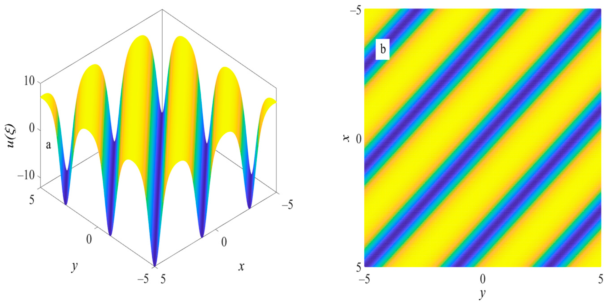
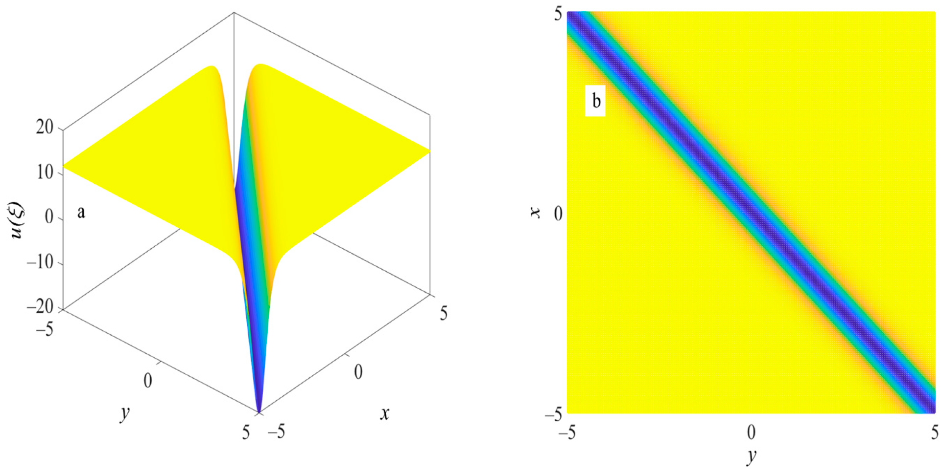
5.1. Periodic Wave Structure and Solitary Wave Structure

If we take $\xi =kx+l\mathrm{y}+\omega t$, we can get the periodic wave structure shown in Figure 1 and the solitary wave structure shown in Figure 2. They are common traveling wave solutions with periodic changes and dark solitary wave solutions. Since the wave structure of $v\left(\xi \right)$ is consistent with that of $u\left(\xi \right)$ in this condition, we have not given its figure.

.

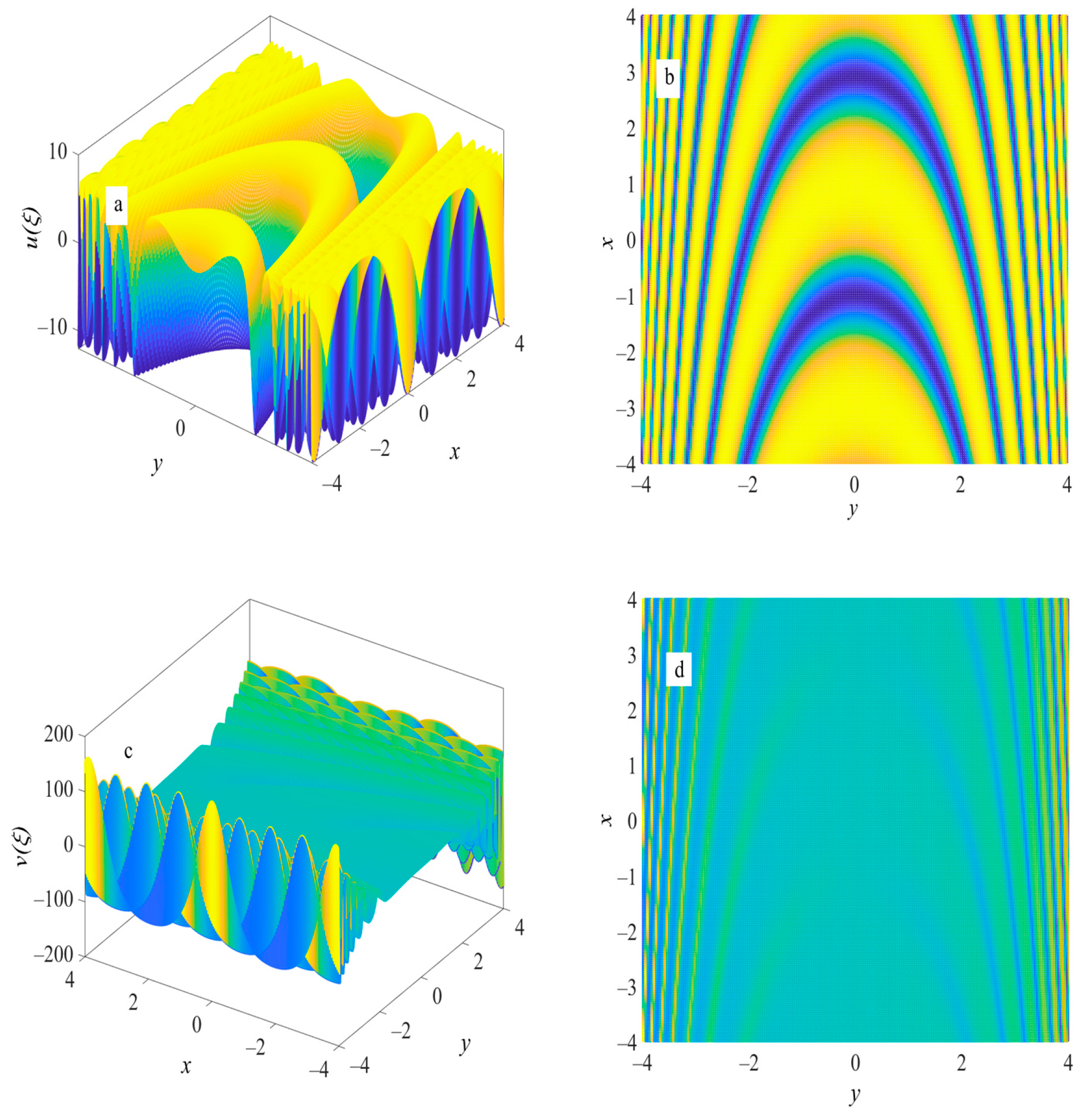
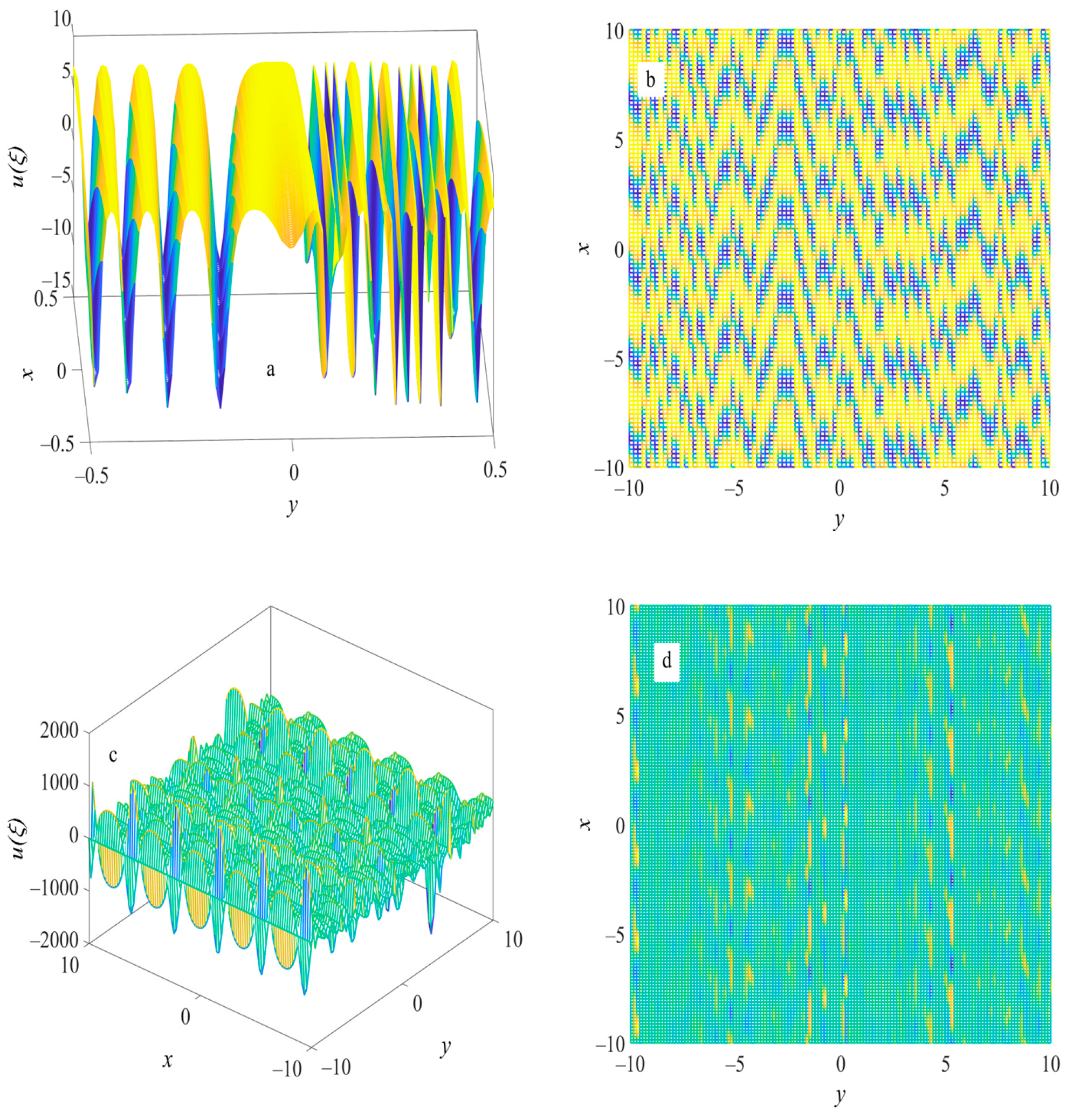
5.2. Complex Wave Structure

If we choose $\xi =kx+\cos \mathrm{h}\left(y\right)+\omega t$, Equations (35) and (36) are the complex wave solutions of the superposition of periodic waves and solitary waves. As a result, we can obtain a horseshoe-type wave structure of Equation (35) as shown in Figure 3a,b and a complex wave structure of Equation (36) as shown in Figure 3c,d with the parameters $k=2, m=0.6, \lambda =1, t=1$ and $\omega =16$.

If we choose $\xi =kx+\sin \left(y\right)+\omega t$, Equations (35) and (36) are the complex wave solutions of the superposition of two kinds of periodic waves. As a result, we can obtain an s-type wave structure of Equation (35) shown in Figure 4a,b, and a breather wave structure of Equation (36) shown in Figure 4c,d with the parameters $k=2, m=0.6, \lambda =1, t=1$ and $\omega =14$.

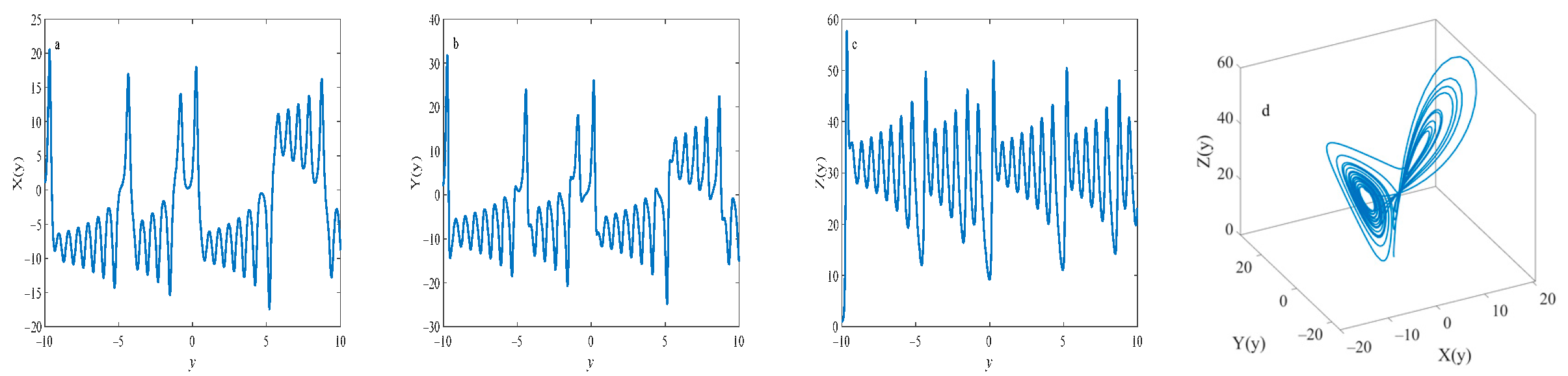
5.3. Chaotic Wave Structure

If we set the arbitrary function $\mathsf{\Phi }\left(y,t\right)$ as the solution of a chaotic dynamic system, we can obtain the chaotic wave structure of the (2+1) dimensional aNNV equation. In this paper, we consider the following Lorenz chaotic dynamic system [39]:

$$\{\begin{array}{c}\frac{dX\left(y\right)}{dy}=a\left[Y\left(y\right)-X\left(y\right)\right], \\ \frac{dY\left(y\right)}{dy}=bX\left(y\right)-Y\left(y\right)-X\left(y\right)Z\left(y\right),\\ \frac{dZ\left(y\right)}{dy}=X\left(y\right)Y\left(y\right)-cZ\left(y\right), \end{array}$$

(53)

where X $\left(y\right)$, Y $\left(y\right)$ and Z $\left(y\right)$ are all functions of y, a, b and c, and they are system parameters.

In this system, there are random and irregular motions, and their behaviors are uncertain, unrepeatable and unpredictable, which is called chaos. Chaos is an inherent characteristic of nonlinear dynamic systems and a universal phenomenon in nonlinear systems. The research of chaos theory is not only of great scientific significance, but also of wide application in mathematical physics. Chaos theory involves almost all fields of natural science and social science and becomes an effective tool to explain or solve complex nonlinear problems. Figure 5 depicts the plot of a typical Lorenz chaotic system with the parameters $a=8, b=33, c=2.2, \mathrm{X}\left(0\right)=1, \mathrm{Y}\left(0\right)=2$ and $\mathrm{Z}\left(0\right)=1$, where it can be seen that the chaotic system has uncertain, unrepeatable and unpredictable motion behavior in the three dimensions. With the increase of y, they show several irregular oscillations with gradually increasing amplitude. When the system moves with y, the system only moves in a limited area of three-dimensional space. The motion of the system in this area is chaotic, and the image formed is called a chaotic attractor (see Figure 5d). In the study of solitons, another field of nonlinear physics, NLEEs are usually solved by ordinary traveling wave transformation with the specific wave structure to obtain various traveling wave solutions. When a wave structure replaces this traveling wave structure with uncertain, unrepeatable and unpredictable chaotic behavior, the traveling wave solution with periodic changes shown in Figure 1 will be modulated by this chaotic wave structure. If we choose $\xi =kx+\mathrm{Z}\left(y\right)+\omega t$, then in the y direction, the structure of the wave shows the chaotic behavior shown in Figure 5c, and as a result, we can obtain chaotic wave structures of Equations (35) and (36) shown in Figure 6 with the parameters $k=2, m=0.6, \lambda =1, t=1$ and $\omega =14$. It can be seen that under this condition, the wave structure of the (2+1)-dimensional aNNV system that originally changed periodically presents uncertain, unrepeatable and unpredictable wave structure in the y direction. This means that the solution of the system has diverged, which leads to the chaotic change of u(ξ) in the y direction. This chaotic behavior makes the soliton uncertain, unrepeatable and unpredictable. When $\xi =kx+\mathrm{X}\left(y\right)+\omega t$ and $\xi =kx+\mathrm{Y}\left(y\right)+\omega t$, the obtained chaotic wave structures are similar to Figure 6, so we do not provide them.

5.4. Spiral Wave Structure

If we set the arbitrary function $\mathsf{\Phi }\left(y,t\right)$ as the solution of the following spiral dynamic system,

$$\{\begin{array}{c}X\left(y\right)=aycos \left(b+cy\right),\\ Y\left(y\right)=aysin \left(b+cy\right),\end{array}$$

(54)

where X $\left(y\right)$ and Y $\left(y\right)$ are all functions of y, a, b and c are system parameters, we can obtain the spiral wave structure of the (2+1) dimensional aNNV equation. Figure 7 depicts a typical spiral system plot with the parameters $a=2, b=\frac{\pi }{4}, c=2\pi$. If we set $\xi =kx+\mathrm{x}\left(y\right)+\omega t$, we can obtain spiral wave structures of Equations (35) and (36) shown in Figure 8 with the parameters $k=2, m=0.6, \lambda =1, t=1$ and $\omega =14$. Because the spiral wave is approximately symmetric, the (2+1) dimensional aNNV system also exhibits an approximately symmetric wave structure. When $\xi =kx+\mathrm{y}\left(y\right)+\omega$, the obtained spiral wave structures are similar to Figure 8, so we do not provide them.

There are still a large number of new types of Jacobian elliptic function solutions for the (2+1)-dimensional aNNV equation, which may also include corresponding hyperbolic function solutions and trigonometric function solutions according to Equations (20)–(29) and table (1), as well as a variety of complex wave structures corresponding to different $\mathsf{\Phi }\left(y,t\right)$. Confined to space, we do not provide examples one by one.

6. Conclusions and Discussion

In this paper, we have constructed a great many Jacobian elliptic function solutions of the (2+1)-dimensional aNNV equation by using a new extended Jacobian elliptic function expansion method. All solutions obtained by this paper have been checked by MATLAB 2021b. (MathWorks, Natick, MA, United States) The transformation of Equations (5) and (7) is the new construction method of solutions proposed by us for the first time, which makes most of the Jacobian elliptic function solutions Equations (20)–(29) obtained are new types of ones. The arbitrary wave transformation Equation (10) makes the obtained solutions have a variety of complex wave structures. To provide more intuitive physical images of these solutions, the various wave structures of a group of solutions are also provided, including periodic wave, solitary wave, complex wave, chaotic wave and spiral wave. Under the condition of ordinary traveling wave transformation, the (2+1)-dimensional aNNV system exhibits solitary wave and periodic wave phenomena. Since the arbitrary wave is a wave structure that can be constructed arbitrarily, we also discussed the complex wave phenomenon of the superposition of two kinds of periodic waves and the superposition of periodic waves and solitary waves. They show horseshoe wave, s-type, and breather wave structures, respectively. We also construct chaotic and spiral wave solutions to explore more complex nonlinear wave phenomena. Under the condition of the chaotic wave, the (2+1)-dimensional aNNV system exhibits uncertain, unrepeatable and unpredictable wave structure in the y direction. Under the spiral wave condition, the system exhibits an approximately symmetric wave structure. These images show the complex nonlinear wave phenomena of the corresponding solution and arbitrary wave transformation. This paper uses the Jacobian elliptic equation as an auxiliary equation to construct the exact solution of NLEEs. Since the Jacobian elliptic equation can construct various complex exact solutions, this method is effective and powerful. It can be used to deal with a broad class of nonlinear problems in the study of mathematics and physics. In addition, our method can also simplify the solving process of NLEEs and construct various nonlinear wave phenomena. In the next work, we will try to use this method to explore more complex nonlinear systems, such as the nonlinear equation with n = 3 and construct more nonlinear wave phenomena. We will also try to apply the solutions of (2+1)-dimensional aNNV system obtained in the previous content to specific fields, such as plasma physics, and try to discuss how this method can be applied to fractional aNNV systems.

References

1. Guo, H.-D.; Xia, T.-C.; Hu, B.-B. High-order lumps, high-order breathers and hybrid solutions for an extended (3+1)-dimensional Jimbo-Miwa equation in fluid dynamics. Nonlinear Dyn. 2020, 100, 601. [Google Scholar] [CrossRef]
2. Lan, Z.-Z.; Guo, B.-L. Nonlinear waves behaviors for a coupled generalized nonlinear Schrodinger-Boussinesq system in a hom generous magnetized plasma. Nonlinear Dyn. 2020, 100, 3771. [Google Scholar] [CrossRef]
3. Biswas, A.; Ekici, M.; Sonmezoglu, A.; Belic, M.R. Solitons in optical fiber Bragg gratings with dispersive reflectivity by extended trial function method. Optik 2019, 182, 88. [Google Scholar] [CrossRef]
4. Seadawy, A.R.; Lu, D.; Nasreen, N.; Nasreen, S. Structure of optical solitons of resonant Schrodinger equation with quadratic cubic nonlinearity and modulation instability analysis. Phys. A Stat. Mech. Its Appl. 2019, 534, 122155. [Google Scholar] [CrossRef]
5. Abdoud, M.A.; Owyed, S.; Abdel-Aty, A.; Raffan, B.M.; Abdel-Khalek, S. Optical soliton solutions for a space-time fractional perturbed nonlinear Schrödinger equation arising in quantum physics. Results Phys. 2020, 16, 102895. [Google Scholar] [CrossRef]
6. Peng, W.-Q.; Tian, S.-F.; Zhang, T.-T. Dynamics of the soliton waves, breather waves, and rogue waves to the cylindrical Kadomtsev-Petviashvili equation in pair-ion-electron plasma. Phys. Fluids 2019, 31, 102107. [Google Scholar] [CrossRef]
7. Wazwaz, A.-M. The extended tanh method for new compact and noncompact solutions for the KP–BBM and the ZK–BBM equations. Chaos Solitons Fractals 2008, 38, 1505. [Google Scholar] [CrossRef]
8. Yusofoǧlu, E. New solitonary solutions for the MBBM equations using Exp-function method. Phys. Lett. A 2008, 372, 442. [Google Scholar] [CrossRef]
9. Gardner, C.S.; Greene, J.M.; Kruskal, M.D.; Miura, R.M. Method for solving Korteweg-de Vries equation. Phys. Rev. Lett. 1967, 19, 1095. [Google Scholar] [CrossRef]
10. Su, C.H.; Gardner, C.S. Korteweg-de Vries Equation and Generalizations. III. Derivation of the Korteweg-de Vries Equation and Burgers Equation. J. Math. Phys. 1969, 10, 536. [Google Scholar] [CrossRef]
11. Li, Z.B.; Wang, M.L. Travelling wave solutions to the two-dimensional KdV-Burgers equation. J. Phy. A: Math. Gen. 1993, 26, 6027. [Google Scholar] [CrossRef]
12. Ito, M. An Extension of Nonlinear Evolution Equations of the K-dV (mK-dV) Type to Higher Orders. J. Phys. Soc. Jpn. 1980, 49, 771. [Google Scholar] [CrossRef]
13. Wang, M. Solitary wave solutions for variant Boussinesq equations. Phys. Lett. A 1995, 199, 169. [Google Scholar] [CrossRef]
14. Yan, C. A simple transformation for nonlinear waves. Phys. Lett. A 1996, 224, 77. [Google Scholar] [CrossRef]
15. Arshad, M.; Seadawy, A.R.; Lu, D.; Wang, J. Travelling wave solutions of Drinfel'd-Sokolov-Wilson, Whitham-Broer-Kaup and (2+1)-dimensional Broer-Kaup-Kupershmit equations and their applications. Chin. J. Phys. 2017, 55, 780. [Google Scholar] [CrossRef]
16. Seadawy, A.R. Stability analysis solutions for nonlinear three-dimensional modified Korteweg-de Vries-Zakharov-Kuznetsov equation in a magnetized electron-positron plasma. Phys. A Stat. Mech. Its Appl. 2016, 455, 44. [Google Scholar] [CrossRef]
17. Liu, J.; Yang, K. The extended F-expansion method and exact solutions of nonlinear PDEs. Chaos Solitons Fractals 2004, 22, 111. [Google Scholar] [CrossRef]
18. Zhang, S. Application of Exp-function method to a KdV equation with variable coefficients. Phys. Lett. A 2007, 365, 448. [Google Scholar] [CrossRef]
19. Seadawy, A.R. Stability analysis for Zakharov-Kuznetsov equation of weakly nonlinear ion-acoustic waves in a plasma. Comput. Math. Appl. 2014, 67, 172. [Google Scholar] [CrossRef]
20. Seadawy, A.R. Stability analysis for two-dimensional ion-acoustic waves in quantum plasmas. Phys. Plasmas 2014, 21, 052107. [Google Scholar] [CrossRef]
21. Shek, E.C.M.; Chow, K.W. The discrete modified Korteweg-de Vries equation with non-vanishing boundary conditions: Interactions of solitons. Chaos Solitons Fractals 2008, 36, 296. [Google Scholar] [CrossRef]
22. Liu, S.; Fu, Z.; Liu, S.; Zhao, Q. Jacobi elliptic function expansion method and periodic wave solutions of nonlinear wave equations. Phys. Lett. A 2001, 289, 69. [Google Scholar] [CrossRef]
23. Boateng, K.; Yang, W.; Yaro, D.; Otoo, M.E. Jacobi Elliptic Function Solutions and Traveling Wave Solutions of the (2+1)-Dimensional Gardner-KP Equation. Math. Methods Appl. Sci. 2020, 43, 3457. [Google Scholar] [CrossRef]
24. Li, H.-M. Searching for the (3+1)-dimensional Painleve integrable model and its solitary wave solution. Chin. Phys. Lett. 2002, 19, 745. [Google Scholar]
25. Yomba, E. On exact solutions of the coupled Klein-Gordon-Schrodinger and the complex coupled KdV equations using mapping method. Chaos Solitons Fractals 2004, 21, 209. [Google Scholar] [CrossRef]
26. Li, H. -M. New exact solutions of nonlinear Gross-Pitaevskii equation with weak bias magnetic and time-dependent laser fields. Chin. Phys. 2005, 14, 251. [Google Scholar] [CrossRef]
27. Wu, G.; Han, J.; Zhang, W.; Zhang, M. New periodic wave solutions to nonlinear evolution equations by the extended mapping method. Phys. D-Nonlinear Phenom. 2007, 229, 116. [Google Scholar] [CrossRef]
28. Zhu, X.; Cheng, J.; Chen, Z.; Wu, G. New Solitary-Wave Solutions of the Van der Waals Normal Form for Granular Materials via New Auxiliary Equation Method. Mathematics 2022, 10, 2560. [Google Scholar] [CrossRef]
29. Tariq, K.U.-H.; Seadawy, A.R. Bistable Bright-Dark solitary wave solutions of the (3 + 1)-dimensional Breaking soliton, Boussinesq equation with dual dispersion and modified Korteweg–de Vries–Kadomtsev–Petviashvili equations and their applications. Results Phys. 2017, 7, 1143. [Google Scholar] [CrossRef]
30. Clarkson, P.A.; Mansfield, E.L. Symmetry reductions and exact solutions of shallow water wave equations. Acta Appl. Math. 1995, 39, 245. [Google Scholar] [CrossRef]
31. Boiti, M.; Leon, J.J.-P.; Manna, M.; Pempinelli, F. On the spectral transrorm of a Korteweg-de Vries equation in two spatial dimensions. Inverse Probl. 1986, 2, 271. [Google Scholar] [CrossRef]
32. Tang, X.-Y.; Lou, S.-Y. A Variable Separation Approach to Solve the Integrable and Nonintegrable Models: Coherent Structures of the (2+1)-Dimensional KdV Equation. Commun. Theor. Phys. 2002, 38, 1. [Google Scholar] [CrossRef]
33. Lou, S.-Y.; Ruan, H.-Y. Revisitation of the localized excitations of the (2+1)-dimensional KdV equation. J. Phys. A: Math. Gen. 2001, 34, 305. [Google Scholar] [CrossRef]
34. Liu, J.-G.; Du, J.-Q.; Zeng, Z.-F.; Ai, G.-P. Exact periodic cross-kink wave solutions for the new (2+1)-dimensional KdV equation in fluid flows and plasma physics. Chaos 2016, 26, 103114. [Google Scholar] [CrossRef] [PubMed]
35. Hossen, M.B.; Roshid, H.-O.; Ali, M.Z. Multi-soliton, breathers, lumps and interaction solution to the (2+1)-dimensional asymmetric Nizhnik-Novikov-Veselov equation. Heliyon 2019, 5, e02548. [Google Scholar] [CrossRef]
36. Zhang, S.; Xia, T. An improved generalized F-expansion method and its application to the (2 + 1)-dimensional KdV equations. Commun. Nonlinear Sci. Numer. Simul. 2008, 13, 1294. [Google Scholar] [CrossRef]
37. Elbrolosy, M.E.; Elmandouh, A.A. Bifurcation and new traveling wave solutions for (2 + 1)-dimensional nonlinear Nizhnik–Novikov–Veselov dynamical equation. Eur. Phys. J. Plus 2020, 135, 533. [Google Scholar] [CrossRef]
38. Mohammed, W.W.; El-Morshedyb, M. The influence of multiplicative noise on the stochastic exact solutions of the Nizhnik–Novikov–Veselov system. Math. Comput. Simul. 2021, 190, 192. [Google Scholar] [CrossRef]
39. Lorenz, E.N. Deterministic Nonperiodic Flow. J. Atmos. Sci. 1963, 20, 130. [Google Scholar] [CrossRef]
Figure 1. (a) Three-dimensional and (b) two-dimensional plots represent the periodic wave solution of Equation (35) when  k = 2 ,   l = 1 ,   m = 0.6 ,   λ = 1 ,   t = 1  and  ω = 14 .
Fractalfract 07 00170 g001
Figure 2. (a) Three-dimensional and (b) two-dimensional contour plots represent the dark solitary wave solution of Equation (35) when  k = 2 ,   l = 1 ,   m = 1 ,   λ = 1 ,   t = 1  and  ω = 14 .
Fractalfract 07 00170 g002
Figure 3. (a) Three-dimensional and (b) two-dimensional contour plots represent the horseshoe-type wave solution of Equation (35) and (c) three-dimensional and (d) two-dimensional contour plots represent the complex wave solution of Equation (36) when  k = 2 ,     m = 0.6 ,   λ = 1 ,   t = 1  and  ω = 16 .
Fractalfract 07 00170 g003
Figure 4. (a) Three-dimensional and (b) two-dimensional contour plots represent the s-type wave structure of Equation (35) and (c) three-dimensional and (d) two-dimensional contour plots represent the breather wave structure of Equation (36) when  k = 2 ,     m = 0.6 ,   λ = 1 ,   t = 1  and  ω = 16 .
Fractalfract 07 00170 g004
Figure 5. A typical plot of Lorenz chaotic dynamic system when  a = 8 ,     b = 33 ,   c = 2.2 ,   X ( 0 ) = 1 ,   Y ( 0 ) = 2  and  Z ( 0 ) = 1 , chaotic solutions of X(y) (a), Y(y) (b), Z(y) (c) and chaotic attractor system (d).
Fractalfract 07 00170 g005
Figure 6. (a) Three-dimensional and (b) two-dimensional contour plots represent the chaotic wave structure of Equation (35) and (c) three-dimensional and (d) two-dimensional contour plots represent the chaotic wave structure of Equation (36) when  k = 2 ,     m = 0.6 ,   λ = 1 ,   t = 1  and  ω = 14 .
Fractalfract 07 00170 g006
Figure 7. A typical plot of the dynamic spiral system when    a = 2 ,     b = π 4  and  c = 2 π , spiral solutions of X(y) (a), Y(y) (b) and spiral system (c).
Fractalfract 07 00170 g007
Figure 8. (a) Three-dimensional and (b) two-dimensional contour plots represent the spiral wave structure of Equation (35) and (c) three-dimensional and (d) two-dimensional contour plots represent the spiral wave structure of Equation (36) when  k = 2 ,     m = 1 ,   λ = 1 ,   t = 1  and  ω = 14 .
Fractalfract 07 00170 g008