


The Fractional Discrete Predator–Prey Model: Chaos, Control and Synchronization

 , ,
, ,
Abstract
1. Introduction
2. Mathematical Model
3. Commensurate Fractional Discrete System
4. Incommensurate Fractional Discrete System
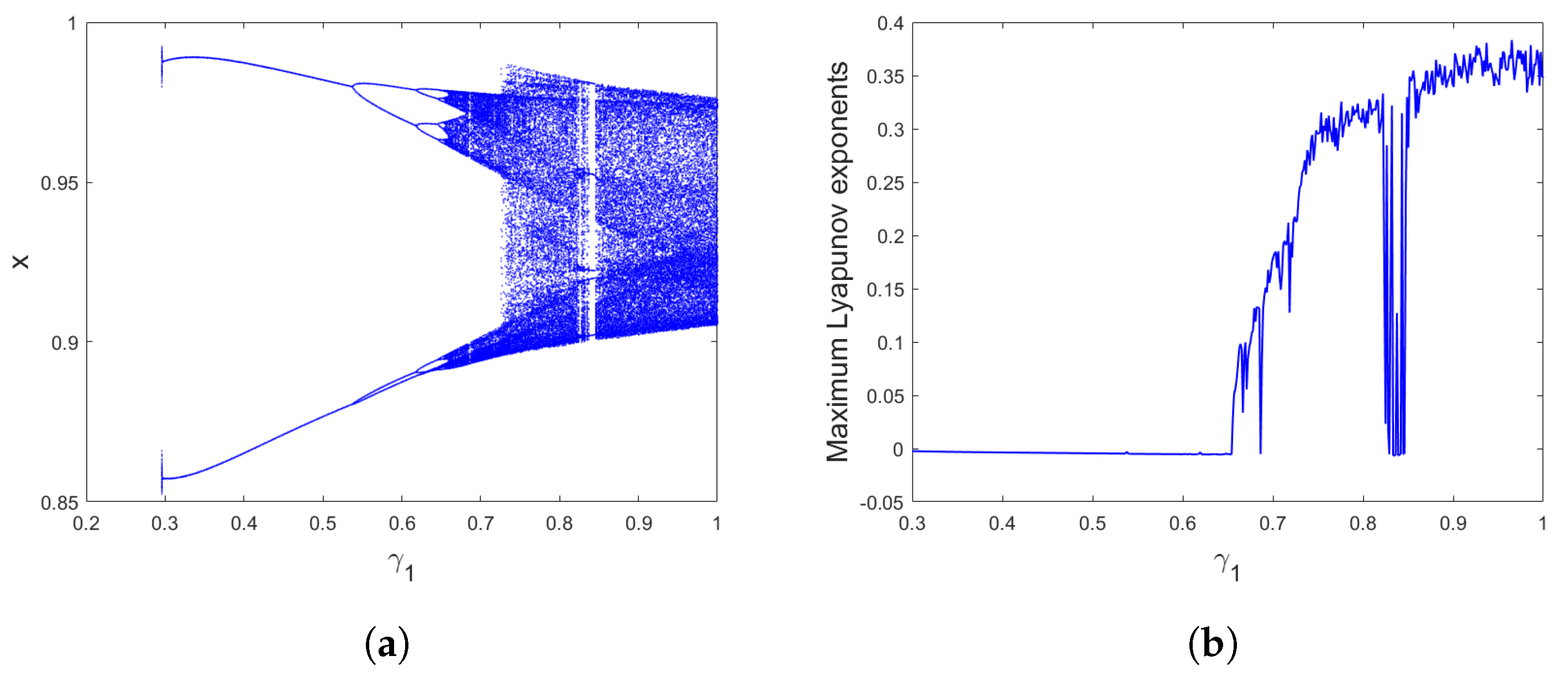
- Case 1.
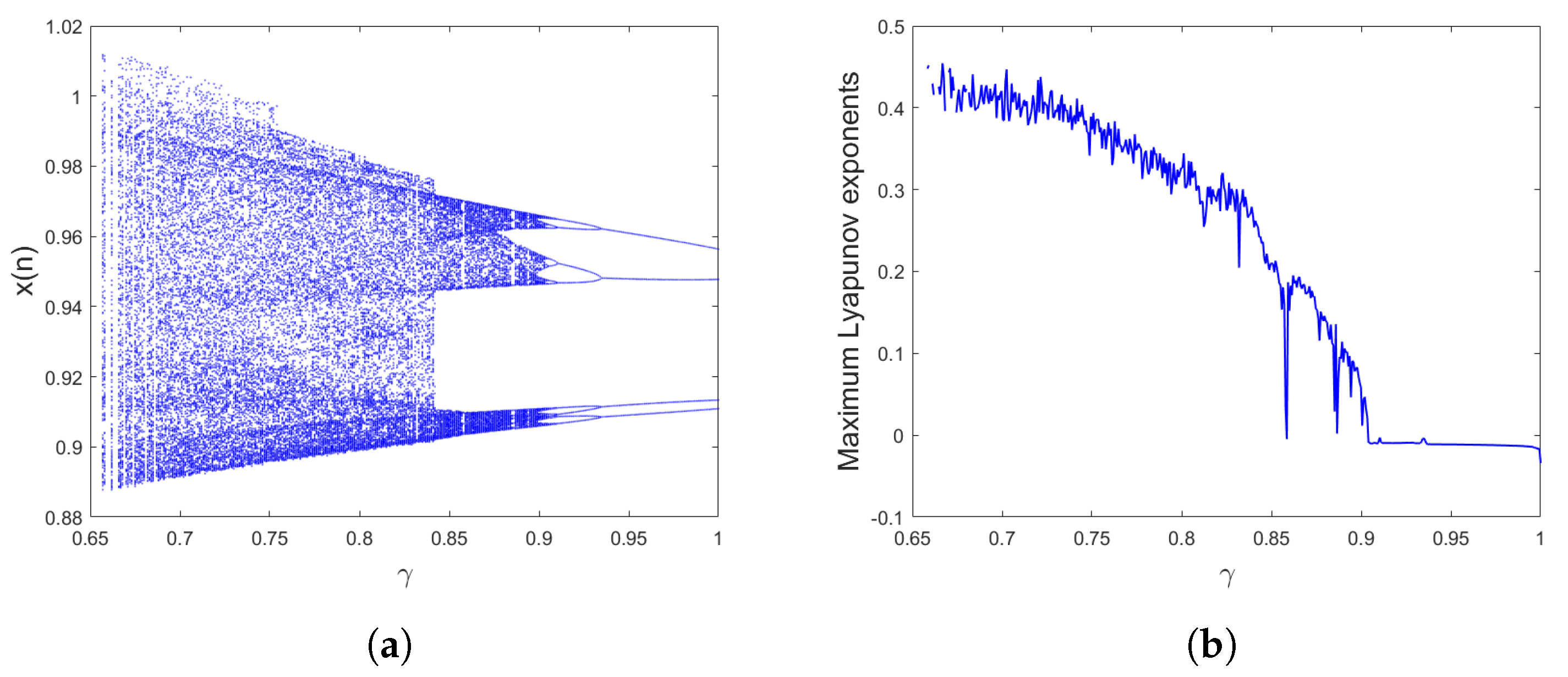
- We vary the order from 0.3 to 1 with step size . Figure 5a,b illustrates the bifurcation and its corresponding MILEs for , the parameter values and initial conditions . It is clear from Figure 5 that the state of the incommensurate map (11) displays chaotic behavior for larger values, as reflected by positive Lyapunov exponents, as seen in Figure 5b. The obtained MLE is 0.383. The Lyapunov exponent shown in Figure 5b is negative for the fractional order value . This result means that a small periodic region is seen for . Moreover, when grows larger and approaches 1, the incommensurate fractional map possesses a complex chaotic attractor as its MLEs reach their maximum values.
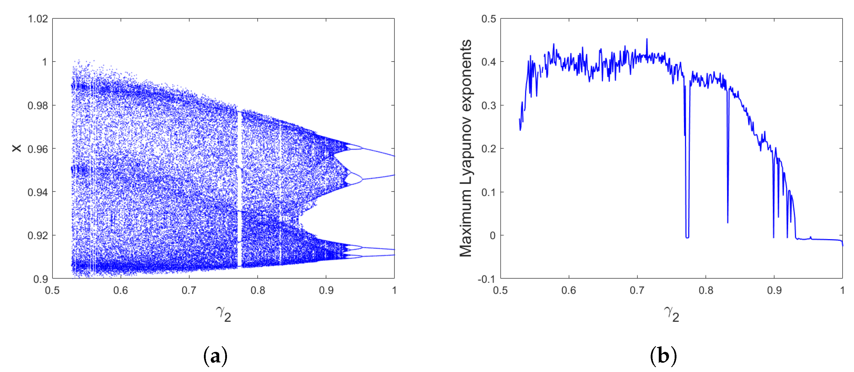
- Case 2.
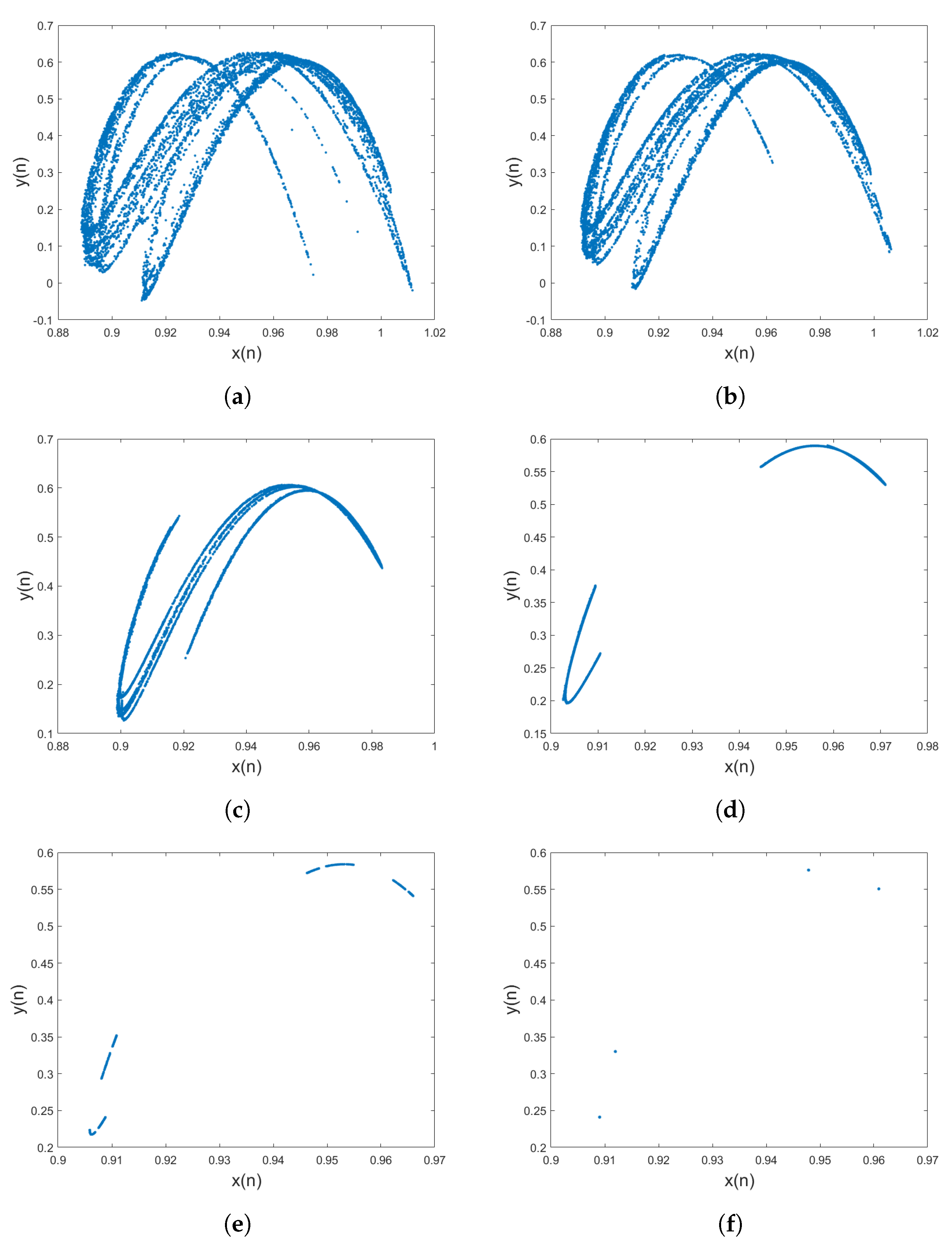
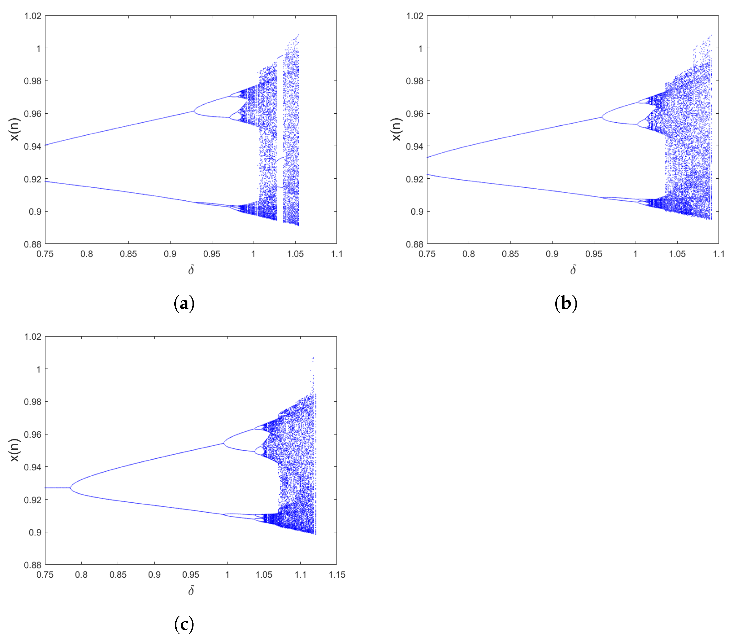
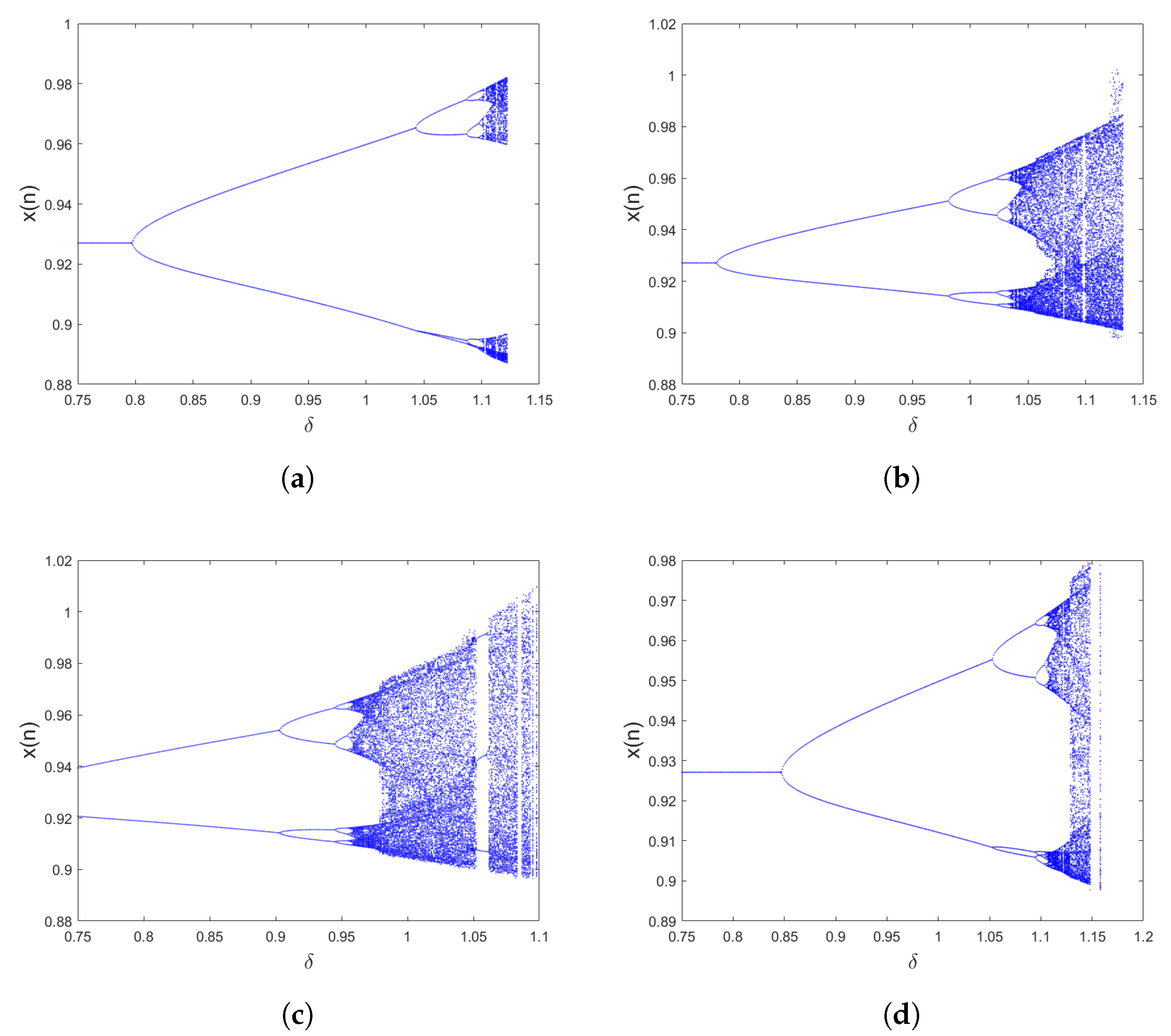
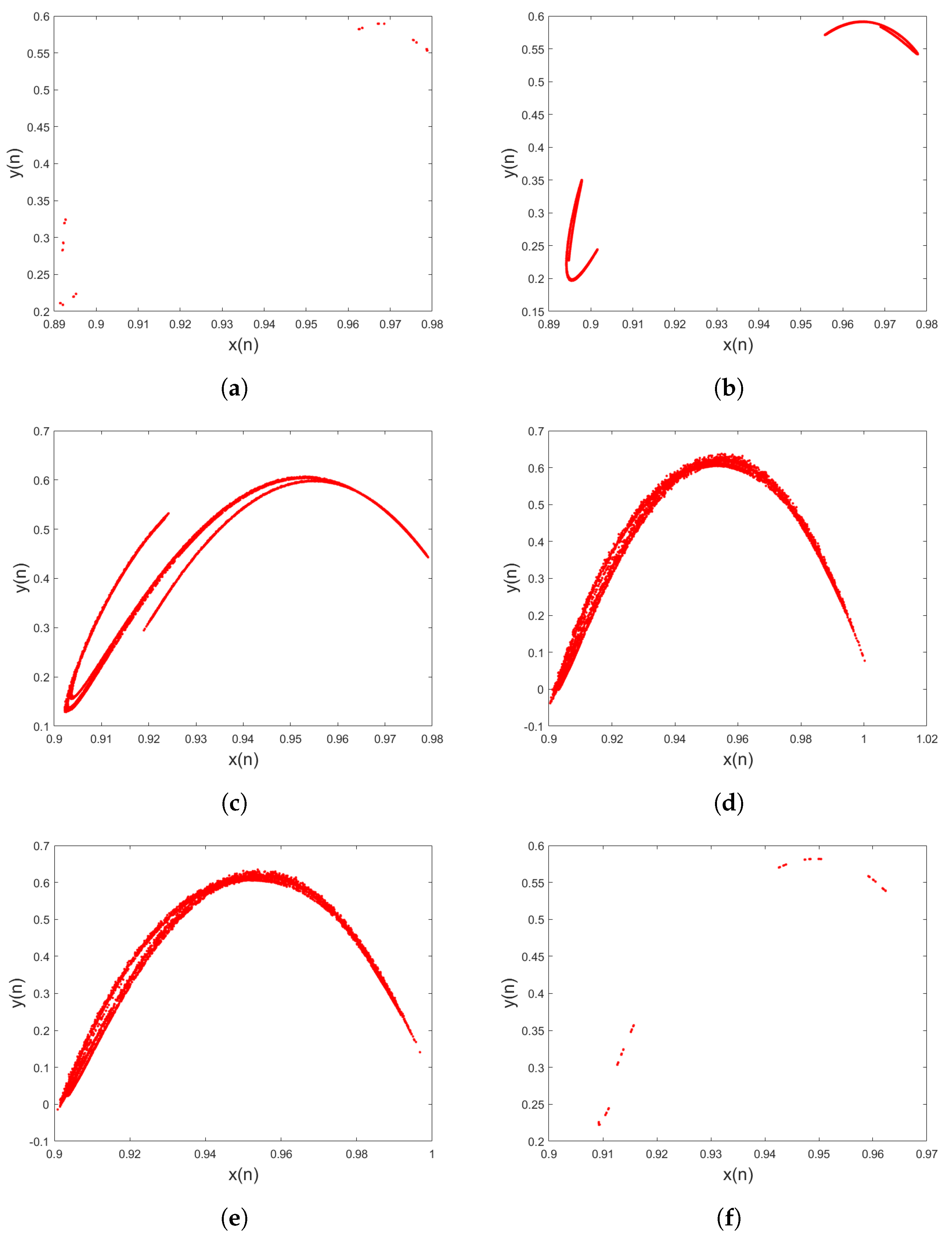
- The bifurcation and its MLE are drawn for to examine the dynamic behaviours of the incommensurate fractional predator–prey discrete system of the Leslie type (11) when is an adjasable parameter, as displayed in Figure 6. These results are obtained by varying in the range and with order . The initial conditions , and the parameter values have remained unchanged. We can observe that when the order has small values, the trajectories will diverge toward infinity. When , chaotic behaviors can be obtained, where the MLE values are positive. A small periodic region is also seen for , where the MLEs have negative values. Moreover, when grows larger and approaches 1, the MLEs are negative, meaning that the incommensurate fractional predator–prey discrete system of Leslie type (11) is stable and periodic windows appear. According to these findings, changes in the incommensurate orders affect the dynamical properties of a fractional predator-prey discrete system of Leslie type. This also suggests that the behaviors of the system may be more accurately represented by incommensurate orders, which is supported by the phase portraits of the state variables of the incommensurate fractional system (11) seen in Figure 7.
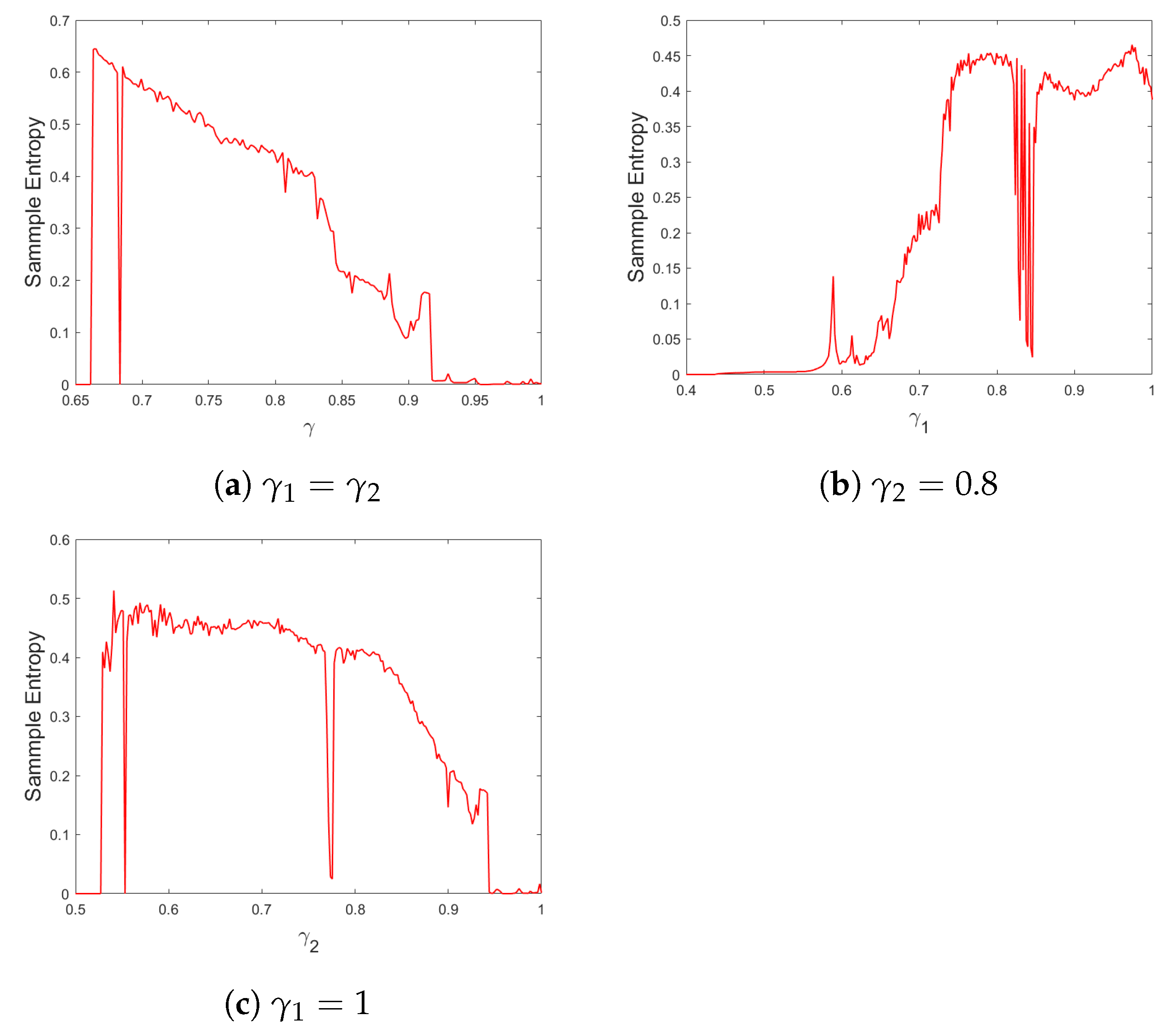
5. The Sample Entropy Test (SampEn)
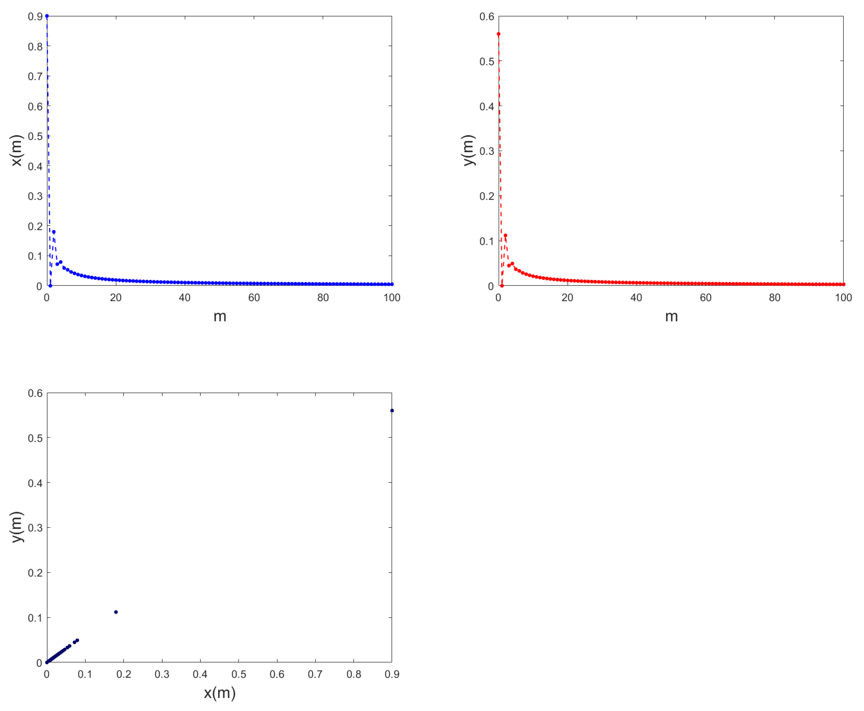
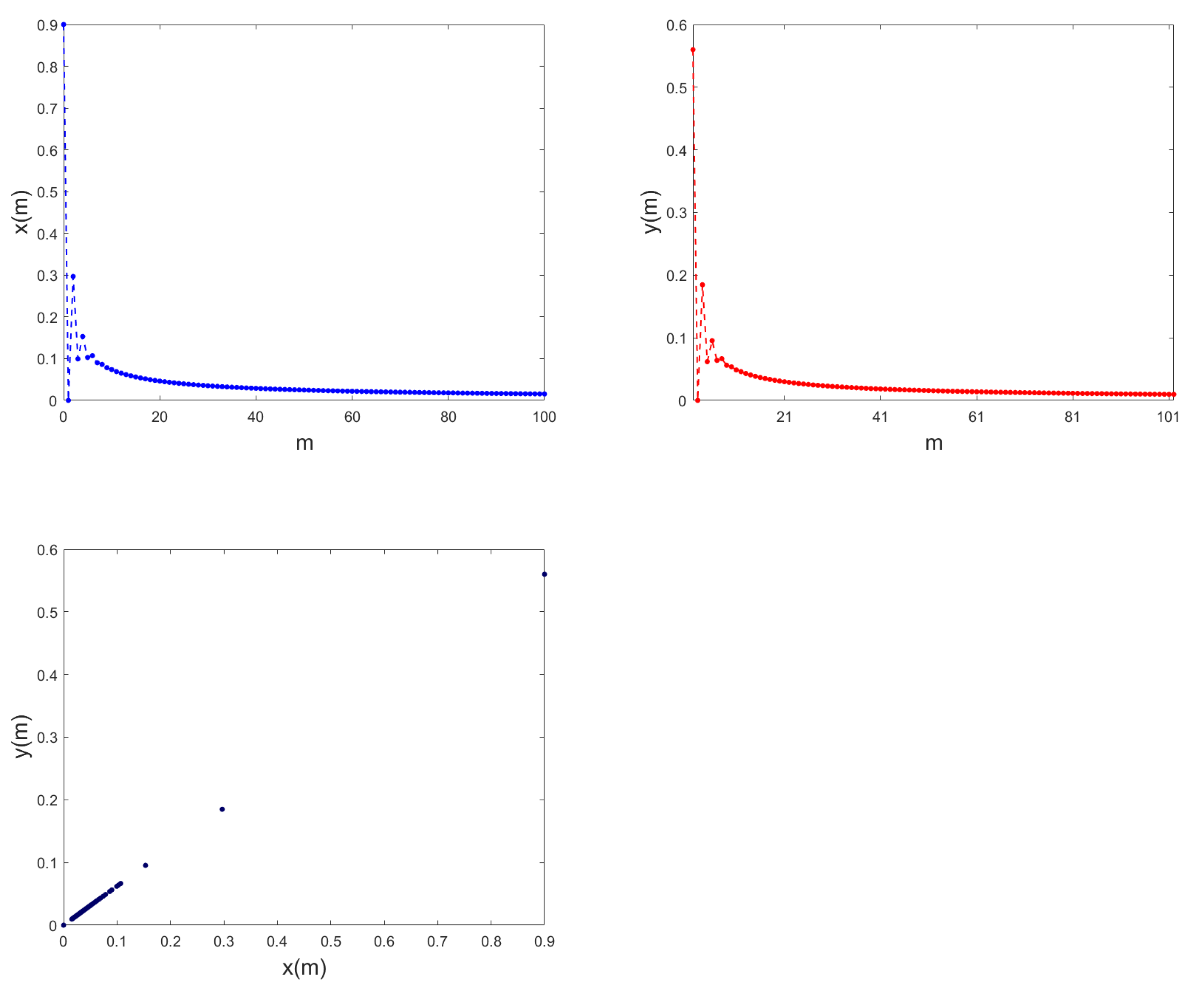
6. Control of Fractional Predator–Prey Discrete System
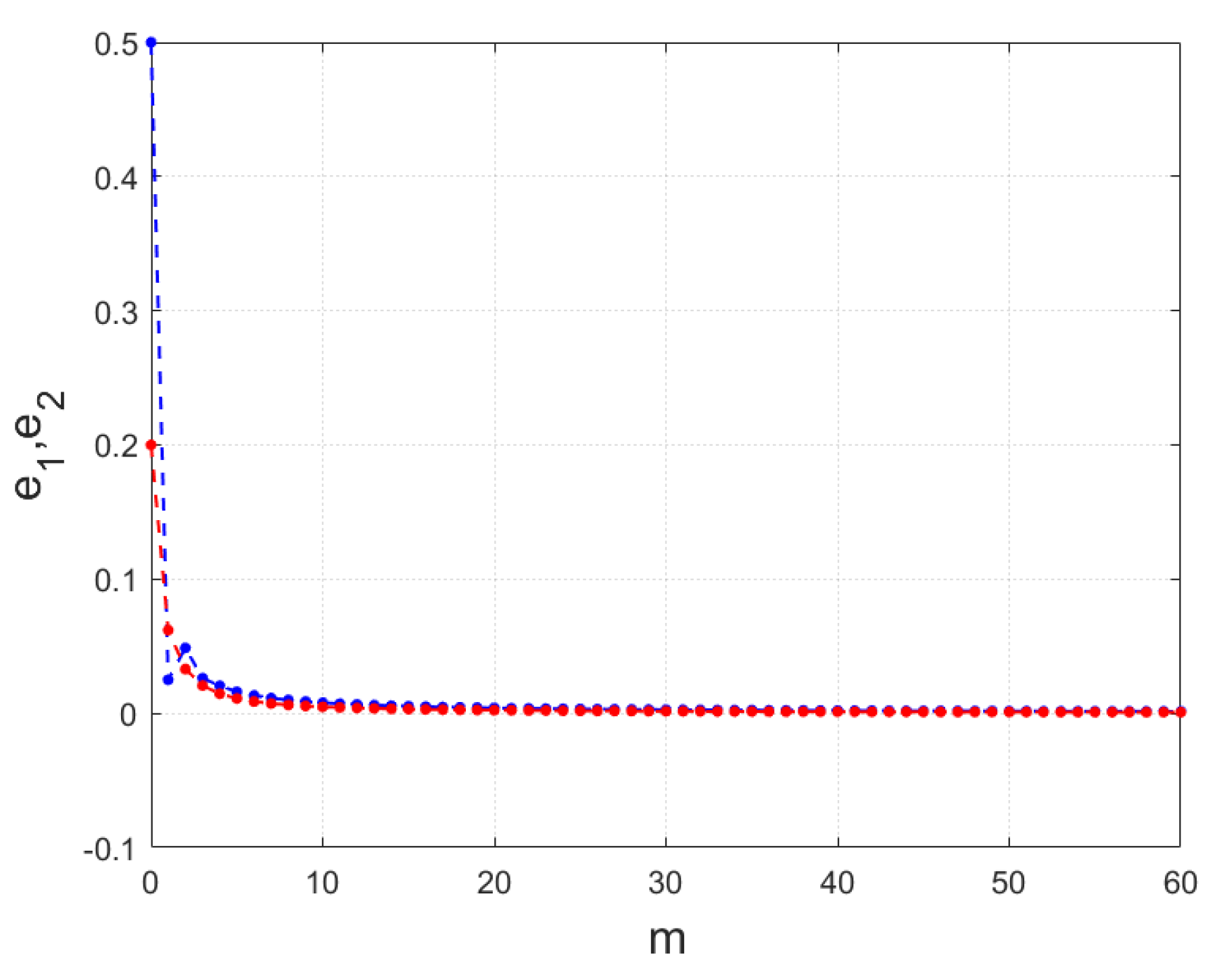
7. Synchronization Scheme
8. Conclusions
Author Contributions
Funding
Institutional Review Board Statement
Informed Consent Statement
Data Availability Statement
Conflicts of Interest
References
- Atici, F.M.; Eloe, P. Discrete fractional calculus with the nabla operator. Electron. J. Qual. Theory Differ. Equ. 2009, 3, 1–12. [Google Scholar] [CrossRef]
- Anastassiou, G.A. Principles of delta fractional calculus on time scales and inequalities. Math. Comput. Model. 2010, 52, 556–566. [Google Scholar] [CrossRef]
- Abdeljawad, T. On Riemann and Caputo fractional differences. Comput. Math. Appl. 2011, 62, 1602–1611. [Google Scholar] [CrossRef]
- Peng, Y.; He, S.; Sun, K. Chaos in the discrete memristor-based system with fractional-order difference. Results Phys. 2021, 24, 104106. [Google Scholar] [CrossRef]
- Khennaoui, A.A.; Ouannas, A.; Momani, S.; Almatroud, O.A.; Al-Sawalha, M.M.; Boulaaras, S.M.; Pham, V.T. Special Fractional-Order Map and Its Realization. Mathematics 2022, 10, 4474. [Google Scholar] [CrossRef]
- Vignesh, D.; Banerjee, S. Dynamical analysis of a fractional discrete-time vocal system. Nonlinear Dyn. 2022, 1–15. [Google Scholar] [CrossRef]
- Shatnawi, M.T.; Abbes, A.; Ouannas, A.; Batiha, I.M. Hidden multistability of fractional discrete non-equilibrium point memristor based map. Physica Scripta 2023. [Google Scholar] [CrossRef]
- Abbes, A.; Ouannas, A.; Shawagfeh, N.; Khennaoui, A.A. Incommensurate Fractional Discrete Neural Network: Chaos and complexity. Eur. Phys. J. Plus 2022, 137, 235. [Google Scholar] [CrossRef]
- Shatnawi, M.T.; Abbes, A.; Ouannas, A.; Batiha, I.M. A new two-dimensional fractional discrete rational map: Chaos and complexity. Phys. Scr. 2022, 98, 015208. [Google Scholar] [CrossRef]
- Abbes, A.; Ouannas, A.; Shawagfeh, N.; Jahanshahi, H. The fractional-order discrete COVID-19 pandemic model: Stability and chaos. Nonlinear Dyn. 2022, 111, 965–983. [Google Scholar] [CrossRef] [PubMed]
- Shatnawi, M.T.; Djenina, N.; Ouannas, A.; Batiha, I.M.; Grassi, G. Novel convenient conditions for the stability of nonlinear incommensurate fractional-order difference systems. Alex Eng. J. 2022, 61, 1655–1663. [Google Scholar] [CrossRef]
- Abbes, A.; Ouannas, A.; Shawagfeh, N.; Grassi, G. The effect of the Caputo fractional difference operator on a new discrete COVID-19 model. Results Phys. 2022, 39, 105797. [Google Scholar] [CrossRef]
- He, Y.; Zheng, S.; Yuan, L. Dynamics of Fractional-Order Digital Manufacturing Supply Chain System and Its Control and Synchronization. Fractal Fract. 2021, 5, 128. [Google Scholar] [CrossRef]
- Zhang, X.L.; Li, H.L.; Kao, Y.; Zhang, L.; Jiang, H. Global Mittag-Leffler synchronization of discrete-time fractional-order neural networks with time delays. Appl. Math. Comput. 2022, 433, 127417. [Google Scholar] [CrossRef]
- Abbes, A.; Ouannas, A.; Shawagfeh, N. Synchronization in Fractional Discrete Neural Networks Using Linear Control Laws. In Proceedings of the 2021 International Conference on Recent Advances in Mathematics and Informatics (ICRAMI), Tebessa, Algeria, 21–22 September2021; pp. 1–5. [Google Scholar]
- Ouannas, A.; Khennaoui, A.A.; Batiha, I.M.; Pham, V.T. Synchronization between fractional chaotic maps with different dimensions. In Emerging Methodologies and Applications in Modelling; Radwan, A.G., Khanday, F.A., Said, L.A., Eds.; Fractional-Order Design; Academic Press: Cambridge, MA, USA, 2022; Volume 3, pp. 89–121. [Google Scholar]
- Hu, D.; Cao, H. Bifurcation and chaos in a discrete-time predator–prey system of Holling and Leslie type. Commun. Nonlinear Sci. Numer. Simul. 2015, 22, 702–715. [Google Scholar] [CrossRef]
- Liu, W.; Jiang, Y. Flip bifurcation and Neimark–Sacker bifurcation in a discrete predator–prey model with harvesting. Int. J. Biomath. 2020, 13, 1950093. [Google Scholar] [CrossRef]
- Rana, S.M.; Kulsum, U. Bifurcation analysis and chaos control in a discrete-time predator-prey system of Leslie type with simplified Holling type IV functional response. Discret. Dyn. Nat. Soc. 2017, 2017, 9705985. [Google Scholar] [CrossRef]
- Khan, A.Q.; Bukhari, S.A.H.; Almatrafi, M.B. Global dynamics, Neimark-Sacker bifurcation and hybrid control in a Leslie’s prey-predator model. Alex. Eng. J. 2022, 61, 11391–11404. [Google Scholar] [CrossRef]
- Chen, J.; Zhu, Z.; He, X.; Chen, F. Bifurcation and chaos in a discrete predator-prey system of Leslie type with Michaelis-Menten prey harvesting. Open Math. 2022, 20, 608–628. [Google Scholar] [CrossRef]
- Wu, G.C.; Baleanu, D. Discrete fractional logistic map and its chaos. Nonlinear Dyn 2014, 75, 283–287. [Google Scholar] [CrossRef]
- Wu, G.C.; Baleanu, D. Jacobian matrix algorithm for Lyapunov exponents of the discrete fractional maps. Commun. Nonlinear Sci. Numer. Simul. 2015, 22, 95–100. [Google Scholar] [CrossRef]
- Richman, J.S.; Moorman, J.R. Physiological time-series analysis using approximate entropy and sample entropy. Am. J. Physiol. Heart Circ. Physiol. 2000, 278, 2039–2049. [Google Scholar] [CrossRef] [PubMed]
- Li, Y.; Wang, X.; Liu, Z.; Liang, X.; Si, S. The entropy algorithm and its variants in the fault diagnosis of rotating machinery: A review. IEEE Access 2018, 6, 66723–66741. [Google Scholar] [CrossRef]
- Čermák, J.; Győri, I.; Nechvátal, L. On explicit stability conditions for a linear fractional difference system. Fract. Calc. Appl. Anal. 2015, 18, 651–672. [Google Scholar] [CrossRef]


| SampEn | SampEn | ||||
|---|---|---|---|---|---|
| 0.67 | 0.67 | 0.6179 | 0.8 | 0.8 | 0.4407 |
| 0.95 | 0.95 | 0.0116 | 1 | 0.6 | 0.4715 |
| 0.65 | 0.8 | 0.0665 | 0.9 | 0.8 | 0.4407 |
| 1 | 0.55 | 0.5017 | 1 | 0.8 | 0.3878 |
Disclaimer/Publisher’s Note: The statements, opinions and data contained in all publications are solely those of the individual author(s) and contributor(s) and not of MDPI and/or the editor(s). MDPI and/or the editor(s) disclaim responsibility for any injury to people or property resulting from any ideas, methods, instructions or products referred to in the content. |
© 2023 by the authors. Licensee MDPI, Basel, Switzerland. This article is an open access article distributed under the terms and conditions of the Creative Commons Attribution (CC BY) license (https://creativecommons.org/licenses/by/4.0/).
Share and Cite
Saadeh, R.; Abbes, A.; Al-Husban, A.; Ouannas, A.; Grassi, G. The Fractional Discrete Predator–Prey Model: Chaos, Control and Synchronization. Fractal Fract. 2023, 7, 120. https://doi.org/10.3390/fractalfract7020120
Saadeh R, Abbes A, Al-Husban A, Ouannas A, Grassi G. The Fractional Discrete Predator–Prey Model: Chaos, Control and Synchronization. Fractal and Fractional. 2023; 7(2):120. https://doi.org/10.3390/fractalfract7020120
Chicago/Turabian StyleSaadeh, Rania, Abderrahmane Abbes, Abdallah Al-Husban, Adel Ouannas, and Giuseppe Grassi. 2023. "The Fractional Discrete Predator–Prey Model: Chaos, Control and Synchronization" Fractal and Fractional 7, no. 2: 120. https://doi.org/10.3390/fractalfract7020120
APA StyleSaadeh, R., Abbes, A., Al-Husban, A., Ouannas, A., & Grassi, G. (2023). The Fractional Discrete Predator–Prey Model: Chaos, Control and Synchronization. Fractal and Fractional, 7(2), 120. https://doi.org/10.3390/fractalfract7020120