
Fixed-Time Distributed Time-Varying Optimization for Nonlinear Fractional-Order Multiagent Systems with Unbalanced Digraphs


Abstract
:1. Introduction
1.1. Related Work and Its Limitations
1.2. Research Motivation
1.3. Research Contribution
- A fixed-time optimal convergence protocol independent of any initial states is designed; this is different from the designed asymptotic optimal convergence protocols in [5,30,37], and the finite-time optimal convergence protocols in [3,14,15] dependent of initial states. However, the fixed-time optimal convergence protocols are designed in [16,17,18,19], where the considered topologies among agents are undirected.
- A weight-unbalanced directed topology without employing certain additional information is considered, which includes the undirected topologies considered in [8,16,18], weight-balanced directed topologies in [19,21,30], and weight-unbalanced directed topologies, and employs certain additional information in [23,24,25,26] as its special cases. However, the weight-unbalanced directed topology without employing certain additional information is considered in [5,27], where the designed protocols are only asymptotic optimal convergence.
- An FOMAS with time-varying local cost functions, heterogeneous unknown nonlinear functions and disturbances is investigated; this is in contrast to the studied MAS with linear and homogeneous integer-order dynamics in [9,12,28,29]. Note that each local cost function is required to be convex in [8,11,12,13,29], strongly convex in [5,17,27,37], and the Hessian of each local cost function is forced to be invertible and equal in [9,10,11,13,37]. However, in this paper, only the global cost function is forced to be convex but not necessarily each local cost function, and only the Hessian of the global cost function is forced to be invertible but not necessarily the Hessian of each local cost function.
2. Preliminaries
2.1. Notations
2.2. Fractional Integral and Derivative
2.3. Directed Graph Theories
2.4. Some Supporting Lemmas
3. Problem Statement
4. Fixed-Time Sliding Mode Control
5. Main Results
5.1. Centralized Fixed-Time Optimization Protocol Design
5.2. Distributed Fixed-Time Optimization Protocol Design
| Algorithm 1: Fixed-time distributed optimization algorithm: A fractional-stage implementation |
|
If Assumptions 1–3 are satisfied, the whole fixed-time distributed optimization procedure is summarized by the following four cascading stages.
▸ Stage 1: Fixed-time estimator of the centralized optimization term : upgrade (5) using (7) with (8), (15), (30) and (31). According to Lemma 6, as , the distributed optimization term given in (31) is equivalent to the centralized optimization term given in (16) for each . ▸ Stage 2: Fixed-time sliding mode control: continue upgrading (5) using (7) with (8), (15), (30) and (31). According to Theorem 1, as , the dynamics of each agent is described by the single-integrator MAS (13). ▸ Stage 3: Fixed-time consensus of , : continue upgrading (5) using (7) with (8), (15), (30) and (31). According to the proof of Step 1 in Theorem 2, as , , . ▸ Stage 4: Fixed-time convergence of , : continue upgrading (5) using (7) with (8), (15), (30) and (31). According to the proof of Step 2 in Theorem 2, as , , . |
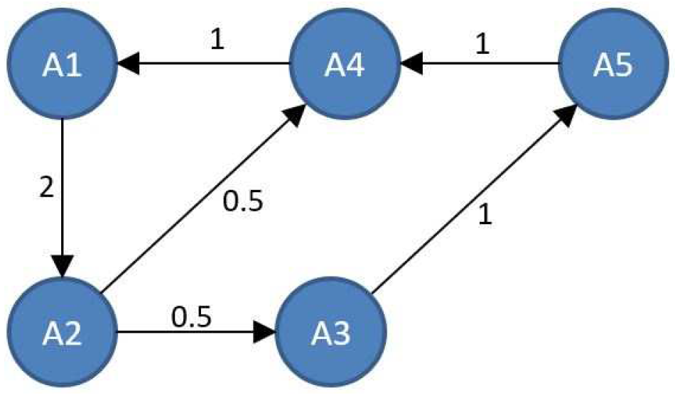
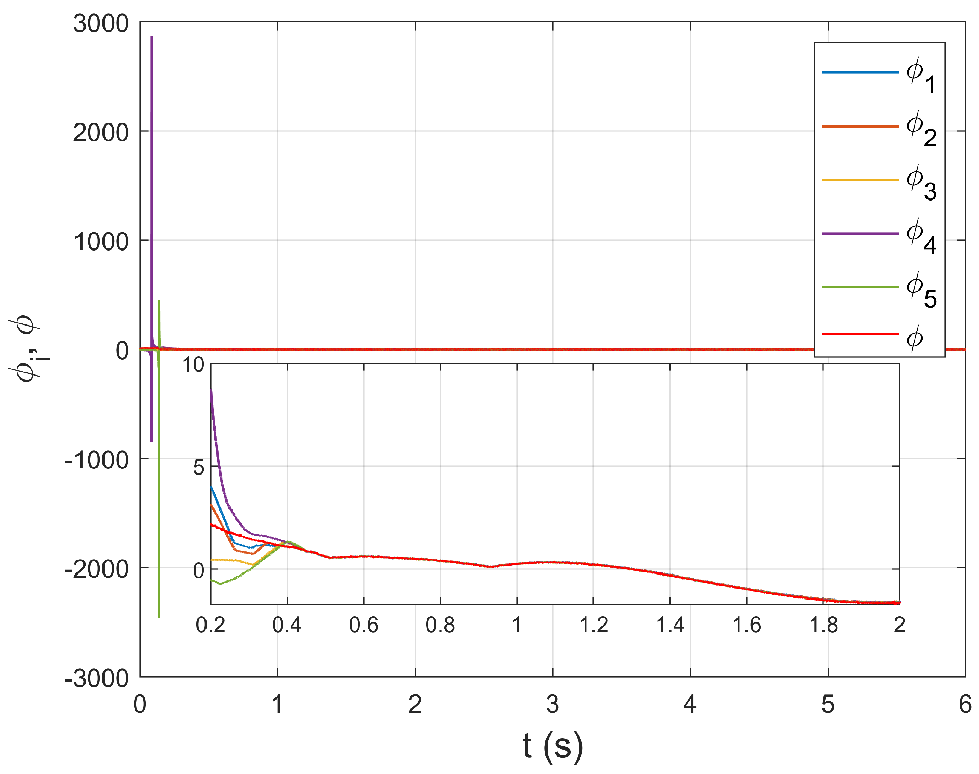
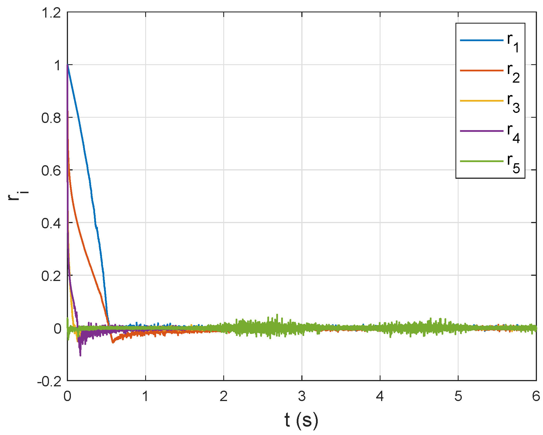
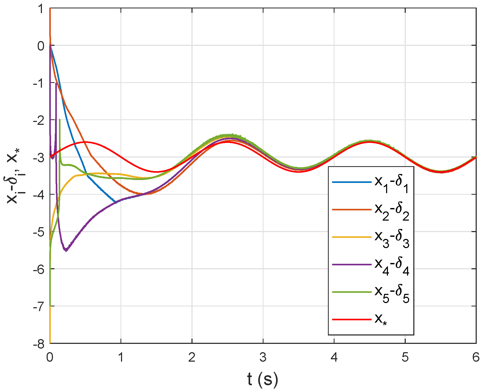
6. Simulation Study
7. Conclusions
Author Contributions
Funding
Data Availability Statement
Conflicts of Interest
References
- Li, C.; Elia, N. Stochastic sensor scheduling via distributed convex optimization. Automatica 2015, 58, 173–182. [Google Scholar] [CrossRef]
- Chen, F.; Chen, X.; Xiang, L.; Ren, W. Distributed economic dispatch via a predictive scheme: Heterogeneous delays and privacy preservation. Automatica 2021, 123, 109356. [Google Scholar] [CrossRef]
- Mao, S.; Dong, Z.; Schultz, P.; Tang, Y.; Meng, K.; Dong, Z.Y.; Qian, F. A finite-time distributed optimization algorithm for economic dispatch in smart grids. IEEE Trans. Syst. Man Cybern. Syst. 2019, 51, 2068–2079. [Google Scholar] [CrossRef]
- Lee, H.; Lee, S.H.; Quek, T.Q. Deep learning for distributed optimization: Applications to wireless resource management. IEEE J. Sel. Areas Commun. 2019, 37, 2251–2266. [Google Scholar] [CrossRef]
- Chen, F.; Jin, J.; Xiang, L.; Ren, W. A scaling-function approach for distributed constrained optimization in unbalanced multiagent networks. IEEE Trans. Autom. Control 2021, 67, 6112–6118. [Google Scholar] [CrossRef]
- Falsone, A.; Margellos, K.; Garatti, S.; Prandini, M. Dual decomposition for multi-agent distributed optimization with coupling constraints. Automatica 2017, 84, 149–158. [Google Scholar] [CrossRef]
- Zhang, Y.; Deng, Z.; Hong, Y. Distributed optimal coordination for multiple heterogeneous Euler-Lagrangian systems. Automatica 2017, 79, 207–213. [Google Scholar] [CrossRef]
- Tran, N.T.; Xiao, J.W.; Wang, Y.W.; Yang, W. Distributed optimisation problem with communication delay and external disturbance. Int. J. Syst. Sci. 2017, 48, 3530–3541. [Google Scholar] [CrossRef]
- Ning, B.; Han, Q.L.; Zuo, Z. Distributed optimization for multiagent systems: An edge-based fixed-time consensus approach. IEEE Trans. Cybern. 2017, 49, 122–132. [Google Scholar] [CrossRef]
- Gong, P.; Chen, F.; Lan, W. Time-varying convex optimization for double-integrator dynamics over a directed network. In Proceedings of the 2016 35th Chinese Control Conference (CCC), Chengdu, China, 27–29 July 2016; pp. 7341–7346. [Google Scholar]
- Hong, H.; Baldi, S.; Yu, W.; Yu, X. Distributed time-varying optimization of second-order multiagent systems under limited interaction ranges. IEEE Trans. Cybern. 2022, 52, 13874–13886. [Google Scholar] [CrossRef]
- Zhao, Y.; Liu, Y.; Wen, G.; Chen, G. Distributed optimization for linear multiagent systems: Edge-and node-based adaptive designs. IEEE Trans. Autom. Control 2017, 62, 3602–3609. [Google Scholar] [CrossRef]
- Huang, B.; Zou, Y.; Meng, Z.; Ren, W. Distributed time-varying convex optimization for a class of nonlinear multiagent systems. IEEE Trans. Autom. Control 2019, 65, 801–808. [Google Scholar] [CrossRef]
- Wang, X.; Wang, G.; Li, S. Distributed finite-time optimization for disturbed second-order multiagent systems. IEEE Trans. Cybern. 2021, 51, 4634–4647. [Google Scholar] [CrossRef] [PubMed]
- Hu, Z.; Yang, J. Distributed finite-time optimization for second order continuous-time multiple agents systems with time-varying cost function. Neurocomputing 2018, 287, 173–184. [Google Scholar] [CrossRef]
- Chen, G.; Li, Z. A fixed-time convergent algorithm for distributed convex optimization in multi-agent systems. Automatica 2018, 95, 539–543. [Google Scholar] [CrossRef]
- Wang, X.; Wang, G.; Li, S. A distributed fixed-time optimization algorithm for multi-agent systems. Automatica 2020, 122, 109289. [Google Scholar] [CrossRef]
- Firouzbahrami, M.; Nobakhti, A. Cooperative fixed-time/finite-time distributed robust optimization of multi-agent systems. Automatica 2022, 142, 110358. [Google Scholar] [CrossRef]
- Li, Y.; He, X.; Xia, D. Distributed fixed-time optimization for multi-agent systems with time-varying objective function. Int. J. Robust Nonlinear Control 2022, 32, 6523–6538. [Google Scholar] [CrossRef]
- Parsegov, S.; Polyakov, A.; Shcherbakov, P. Fixed-time consensus algorithm for multi-agent systems with integrator dynamics. IFAC Proc. Vol. 2013, 46, 110–115. [Google Scholar] [CrossRef]
- Gharesifard, B.; Cortés, J. Distributed continuous-time convex optimization on weight-balanced digraphs. IEEE Trans. Autom. Control 2014, 59, 781–786. [Google Scholar] [CrossRef]
- Makhdoumi, A.; Ozdaglar, A. Graph balancing for distributed subgradient methods over directed graphs. In Proceedings of the 2015 54th IEEE Conference on Decision and Control (CDC), Osaka, Japan, 15–18 December 2015; pp. 1364–1371. [Google Scholar]
- Akbari, M.; Gharesifard, B.; Linder, T. Distributed online convex optimization on time-varying directed graphs. IEEE Trans. Control Netw. Syst. 2017, 4, 417–428. [Google Scholar] [CrossRef]
- Touri, B.; Gharesifard, B. Continuous-time distributed convex optimization on time-varying directed networks. In Proceedings of the 2015 54th IEEE Conference on Decision and Control (CDC), Osaka, Japan, 15–18 December 2015; pp. 724–729. [Google Scholar]
- Li, Z.; Ding, Z.; Sun, J.; Li, Z. Distributed adaptive convex optimization on directed graphs via continuous-time algorithms. IEEE Trans. Autom. Control 2018, 63, 1434–1441. [Google Scholar] [CrossRef]
- Yu, Z.; Yu, S.; Jiang, H.; Mei, X. Distributed fixed-time optimization for multi-agent systems over a directed network. Nonlinear Dyn. 2021, 103, 775–789. [Google Scholar] [CrossRef]
- Zhu, Y.; Yu, W.; Wen, G.; Ren, W. Continuous-time coordination algorithm for distributed convex optimization over weight-unbalanced directed networks. IEEE Trans. Circuits Syst. II Express Briefs 2019, 66, 1202–1206. [Google Scholar] [CrossRef]
- Rahili, S.; Ren, W. Distributed continuous-time convex optimization with time-varying cost functions. IEEE Trans. Autom. Control 2017, 62, 1590–1605. [Google Scholar] [CrossRef]
- Gong, X.; Cui, Y.; Shen, J.; Xiong, J.; Huang, T. Distributed optimization in prescribed-time: Theory and experiment. IEEE Trans. Netw. Sci. Eng. 2022, 9, 564–576. [Google Scholar] [CrossRef]
- Liu, Y.; Yang, G.H. Distributed robust adaptive optimization for nonlinear multiagent systems. IEEE Trans. Syst. Man Cybern. Syst. 2021, 51, 1046–1053. [Google Scholar] [CrossRef]
- Abdelwahed, H.; El-Shewy, E.; Alghanim, S.; Abdelrahman, M.A. On the physical fractional modulations on Langmuir plasma structures. Fractal Fract. 2022, 6, 430. [Google Scholar] [CrossRef]
- Sharaf, M.; El-Shewy, E.; Zahran, M. Fractional anisotropic diffusion equation in cylindrical brush model. J. Taibah Univ. Sci. 2020, 14, 1416–1420. [Google Scholar] [CrossRef]
- Liang, B.; Zheng, S.; Ahn, C.K.; Liu, F. Adaptive fuzzy control for fractional-order interconnected systems with unknown control directions. IEEE Trans. Fuzzy Syst. 2022, 30, 75–87. [Google Scholar] [CrossRef]
- Azar, A.T.; Radwan, A.G.; Vaidyanathan, S. Fractional Order Systems: Optimization, Control, Circuit Realizations and Applications; Academic Press: Cambridge, MA, USA, 2018. [Google Scholar]
- Yang, X.; Zhao, W.; Yuan, J.; Chen, T.; Zhang, C.; Wang, L. Distributed optimization for fractional-order multi-agent systems based on adaptive backstepping dynamic surface control technology. Fractal Fract. 2022, 6, 642. [Google Scholar] [CrossRef]
- Gong, P.; Han, Q.L. Distributed fixed-time optimization for second-order nonlinear multiagent systems: State and output feedback designs. IEEE Trans. Autom. Control 2023. [Google Scholar] [CrossRef]
- Sun, S.; Zhang, Y.; Lin, P.; Ren, W.; Farrell, J.A. Distributed time-varying optimization with state-dependent gains: Algorithms and experiments. IEEE Trans. Control Syst. Technol. 2022, 30, 416–425. [Google Scholar] [CrossRef]
- Podlubny, I. Fractional Differential Equations. In Mathematics in Science and Engineering; Elsevier: Amsterdam, The Netherlands, 1999. [Google Scholar]
- Gong, P.; Han, Q.L. Practical fixed-time bipartite consensus of nonlinear incommensurate fractional-order multiagent systems in directed signed networks. SIAM J. Control Optim. 2020, 58, 3322–3341. [Google Scholar] [CrossRef]
- Li, Z.; Wen, G.; Duan, Z.; Ren, W. Designing fully distributed consensus protocols for linear multi-agent systems with directed graphs. IEEE Trans. Autom. Control 2015, 60, 1152–1157. [Google Scholar] [CrossRef]
- Hardy, G.H.; Littlewood, J.E.; Pólya, G. Inequalities; Cambridge University Press: Cambridge, UK, 1952. [Google Scholar]
- Boyd, S.P.; Vandenberghe, L. Convex Optimization; Cambridge University Press: Cambridge, UK, 2004. [Google Scholar]
- Wang, Y.; Song, Y.; Lewis, F.L. Robust adaptive fault-tolerant control of multiagent systems with uncertain nonidentical dynamics and undetectable actuation failures. IEEE Trans. Ind. Electron. 2015, 62, 3978–3988. [Google Scholar]
- Gong, P.; Lan, W.; Han, Q.L. Robust adaptive fault-tolerant consensus control for uncertain nonlinear fractional-order multi-agent systems with directed topologies. Automatica 2020, 117, 109011. [Google Scholar] [CrossRef]
- Zou, W.; Qian, K.; Xiang, Z. Fixed-time consensus for a class of heterogeneous nonlinear multiagent systems. IEEE Trans. Circuits Syst. II Express Briefs 2020, 67, 1279–1283. [Google Scholar] [CrossRef]


| Related Work | Optimal Convergence Rate | Topology | Dynamics |
|---|---|---|---|
| [11,28,37] | Infinite time | Undirected | Linear |
| [13] | Infinite time | Undirected | Nonlinear |
| [15] | Finite time | Undirected | Linear |
| [19] | Fixed time | Undirected | Linear |
| This work | Fixed time | Directed | Nonlinear |
| j | |||
|---|---|---|---|
| 1 | 2 | ||
| 2 | 0 | ||
| 3 | 4 | ||
| 4 | 0 | ||
| 5 | 0 | ||
| 0 | 1 |
Disclaimer/Publisher’s Note: The statements, opinions and data contained in all publications are solely those of the individual author(s) and contributor(s) and not of MDPI and/or the editor(s). MDPI and/or the editor(s) disclaim responsibility for any injury to people or property resulting from any ideas, methods, instructions or products referred to in the content. |
© 2023 by the authors. Licensee MDPI, Basel, Switzerland. This article is an open access article distributed under the terms and conditions of the Creative Commons Attribution (CC BY) license (https://creativecommons.org/licenses/by/4.0/).
Share and Cite
Wang, K.; Gong, P.; Ma, Z. Fixed-Time Distributed Time-Varying Optimization for Nonlinear Fractional-Order Multiagent Systems with Unbalanced Digraphs. Fractal Fract. 2023, 7, 813. https://doi.org/10.3390/fractalfract7110813
Wang K, Gong P, Ma Z. Fixed-Time Distributed Time-Varying Optimization for Nonlinear Fractional-Order Multiagent Systems with Unbalanced Digraphs. Fractal and Fractional. 2023; 7(11):813. https://doi.org/10.3390/fractalfract7110813
Chicago/Turabian StyleWang, Kun, Ping Gong, and Zhiyao Ma. 2023. "Fixed-Time Distributed Time-Varying Optimization for Nonlinear Fractional-Order Multiagent Systems with Unbalanced Digraphs" Fractal and Fractional 7, no. 11: 813. https://doi.org/10.3390/fractalfract7110813
APA StyleWang, K., Gong, P., & Ma, Z. (2023). Fixed-Time Distributed Time-Varying Optimization for Nonlinear Fractional-Order Multiagent Systems with Unbalanced Digraphs. Fractal and Fractional, 7(11), 813. https://doi.org/10.3390/fractalfract7110813